1 Introduction

Fractional calculus is dedicated to study the integrals and derivatives of any arbitrary real (or complex) order. It has a long history from 1695 [2, 3]. The first book dedicated specifically to study the theory of fractional integrals and derivatives and their applications, is the book by Oldham and Spanier [4] published in 1974. There exists a remarkably comprehensive encyclopedic-type monograph by Samko, Kilbas and Marichev [5]. Many other publications including different fractional models had appeared from 1980. For example, see [6]-[23]. Fractional calculus and the theory of integro-differential equations of non-integer orders are powerful tools to describe the dynamics of anomalous systems and processes with power-law non-locality, long-range memory and/or fractal properties.

Spatial dispersion is called the dependence of the tensor of the absolute permittivity of the medium on the wave vector [24, 25, 26]. This dependence leads to a number of phenomena, such as the rotation of the plane of polarization, anisotropy of cubic crystals and other [27, 28, 29, 30, 31, 32, 33, 34, 35, 36, 37, 38]. The spatial dispersion is caused by non-local connection between the electric induction ${\bf D}$ and the electric field ${\bf E}$. Vector ${\bf D}$ at any point ${\bf r}$ of the medium is not uniquely defined by the values of ${\bf E}$ at this point. It also depends on the values of ${\bf E}$ at neighboring points ${\bf r}^{\prime}$, located near the point ${\bf r}$.

Plasma-like medium is medium in which the presence of free charge carriers, creating as they move in the medium, electric and magnetic fields, which significantly distorts the external field and the effect on the motion of the charges themselves [24, 25, 26]. The term ”plasma-like media” refers to media with high spatial dispersion. These media are ionized gas, metals and semiconductors, molecular crystals and colloidal electrolytes. The term ”plasma-like media” was introduced in 1961, by Viktor P. Silin and Henri A. Rukhadze in the book ”The electromagnetic properties of the plasma and plasma-like media” [24].

In Section 2 the basic concepts and well-known equations of electrodynamics of continuous media are considered to fix the notation. In Section 3, we consider power-law type generalizations of Debye’s permittivity and generalizations of the correspondent equations for electrostatic potential by involving the fractional generalization of the Laplacian. The simplest power-law forms of the longitudinal permittivity and correspondent equations for the electrostatic potential are suggested. The power-law type deformation of Debye’s screening and Coulomb’s law are discussed. These suggested simple models allows us to demonstrate new possible types of an anomalous behavior of media with fractional power-law type of non-locality. In Section 4 the description of weak spatial dispersions of power-law type in the plasma-like media is discussed. The fractional generalizations of the Taylor series are used for this description. The correspondent power-law deformation of Debye’s screening and Coulomb’s law are considered. A short conclusion is given in Section 5. In Appendix 1, we suggest a short introduction to the Riesz fractional derivatives and integrals. In Appendix 2, the fractional Taylor formulas of different types are described.

In this section we review some basic concepts and well-known equations of electrodynamics of continuous media, to fix the notation. For details see [24, 25, 26].

The behavior of electric fields (${\bf E},{\bf D}$), magnetic fields (${\bf B},{\bf H}$), charge density $\rho$, and current density ${\bf j}$ is described by the well-known Maxwell’s equations

$$\operatorname{div}{\bf D}(t,{\bf r})=\rho(t,{\bf r}),$$ (1)

$$\operatorname{curl}{\bf E}(t,{\bf r})=-\frac{\partial{\bf B}(t,{\bf r})}{\partial t},$$ (2)

$$\operatorname{div}{\bf B}(t,{\bf r})=0,$$ (3)

$$\operatorname{curl}{\bf H}(t,{\bf r})={\bf j}(t,{\bf r})+\frac{\partial{\bf D}(t,{\bf r})}{\partial t}.$$ (4)

The densities $\rho(t,{\bf r})$ and ${\bf j}(t,{\bf r})$ describe an external source of field. We assume that the external sources of electromagnetic field are given. The vector ${\bf E}(t,{\bf r})$ is the electric field strength and the vector ${\bf D}(t,{\bf r})$ is the electric displacement field. In free space, the electric displacement field is equivalent to flux density. The field ${\bf B}(t,{\bf r})$ is the magnetic induction and the vector ${\bf H}(t,{\bf r})$ is the magnetic field strength.

In the case of the linear electrodynamics the constitutive equations (material equations) are linear relations. For electromagnetic fields which are changed slowly in the space-time, we have the constitutive equations (material equations) in the well-known form

$$D_{i}(t,{\bf r})=\varepsilon_{ij}E_{j}(t,{\bf r}),$$ (5)

$$B_{i}(t,{\bf r})=\mu_{ij}H_{j}(t,{\bf r}),$$ (6)

where $\varepsilon_{ij}$ and $\mu_{ij}$ are second-rank tensors. For fields varying in space rapidly, we should consider the influence of the field at remote points ${\bf r}^{\prime}$ on the electromagnetic properties of the medium at a given point ${\bf r}$. The field at a given point ${\bf r}$ of the medium will be determined not only the value of the field at this point, but the field in the areas of environment, where the influence of the field is transferred. For example, it can be caused by the transport processes in the medium. Therefore, we should use non-local space relations instead of equations (5), (6). These non-local relations take into account space dispersion. For linear electrodynamics we have the following relation between electric fields ${\bf E}$ and ${\bf D}$ given by

$$D_{i}(t,{\bf r})=\int_{\mathbb{R}^{3}}\hat{\varepsilon}_{ij}({\bf r},{\bf r}^{\prime})\,E_{j}(t,{\bf r}^{\prime})\,d{\bf r}^{\prime},$$ (7)

and

$$B_{i}(t,{\bf r})=\int_{\mathbb{R}^{3}}\hat{\mu}_{ij}({\bf r},{\bf r}^{\prime})\,H_{j}(t,{\bf r}^{\prime})\,d{\bf r}^{\prime}.$$ (8)

If the medium is not limited in space and homogeneous, then the kernel of the integral operator is a function of the position difference ${\bf r}-{\bf r}^{\prime}$,

$$D_{i}(t,{\bf r})=\int_{\mathbb{R}^{3}}\hat{\varepsilon}_{ij}({\bf r}-{\bf r}^{\prime})\,E_{j}(t,{\bf r}^{\prime})\,d{\bf r}^{\prime}.$$ (9)

In this case we can use the Fourier transform. The direct and inverse Fourier transforms ${\cal F}$ and ${\cal F}^{-1}$, for suitable functions, are given by

$$({\cal F}f)({\bf k})={\cal F}[f({\bf r})]({\bf k})=\int_{\mathbb{R}^{3}}e^{-i({\bf k}{\bf r})}\,f({\bf r})\,d^{3}{\bf r},$$ (10)

$$\hat{g}({\bf r})=({\cal F}^{-1}g)({\bf r})={\cal F}^{-1}[g({\bf k})]({\bf r})=\frac{1}{(2\pi)^{3}}\int_{\mathbb{R}^{3}}e^{+i({\bf k}{\bf r})}\,g({\bf k})\,d^{3}{\bf k}.$$ (11)

We does not use the hat for ${\bf D}(t,{\bf r})$ and ${\bf E}(t,{\bf r})$ to have usual notation. From the context, it will be easy to understand if the field is considered in the space-time of its the Fourier transforms.

Then electric field will be represented as a set of plane monochromatic waves, for which space-time dependence are defined by the function $exp\{i{\bf k}{\bf r}-i\omega t\}$. Therefore, relation (9) has the form

$$D_{i}(\omega,{\bf k})=\varepsilon_{ij}({\bf k})E_{j}(\omega,{\bf k}).$$ (12)

The function $\varepsilon_{ij}({\bf k})$ is called the tensor of the absolute permittivity of the material:

$$\varepsilon_{ij}({\bf k})=\int_{\mathbb{R}^{3}}e^{-i{\bf k}{\bf r}}\,\hat{\varepsilon}_{ij}({\bf r})\,d{\bf r}^{\prime}.$$ (13)

Even for an isotropic linear medium, the dependence of the tensor $\varepsilon_{ij}({\bf k})$ of the wave vector ${\bf k}$ preserves tensor form [24, 25, 26]. In this case we have

$$\varepsilon_{ij}({\bf k})=\left(\delta_{ij}-\frac{k_{i}k_{j}}{|{\bf k}|^{2}}\right)\,\varepsilon_{\perp}(|{\bf k}|)+\frac{k_{i}k_{j}}{|{\bf k}|^{2}}\,\varepsilon_{\parallel}(|{\bf k}|),$$ (14)

where $\varepsilon_{\perp}(|{\bf k}|)$ - the transverse permittivity, and $\varepsilon_{\parallel}(|{\bf k}|)$ - the longitudinal permittivity.

The Maxwell’s equations for the electromagnetic fields have the well-known form [24, 25, 26]

$$i({\bf k},{\bf E}(\omega,{\bf k}))\,\varepsilon({\bf k})=\rho(\omega,{\bf k}),$$ (15)

$$[{\bf k},{\bf E}(\omega,{\bf k})]=\omega\,{\bf B}(\omega,{\bf k}),$$ (16)

$$({\bf k},{\bf B}(\omega,{\bf k}))=0,$$ (17)

$$\frac{i}{\mu(\bf k)}\,[{\bf k},{\bf B}(\omega,{\bf k})]=-i\omega\varepsilon({\bf k})\,{\bf E}(\omega,{\bf k})+{\bf j}(\omega,{\bf k}).$$ (18)

In these equations we have neglected the frequency dispersion. This can be done when the inhomogeneous field can be approximately regarded as static.

In the case of a static external field sources in the environment can create a inhomogeneous electric field ${\bf E}(t,{\bf r})={\bf E}({\bf r})$. The electric field in the medium is given by

$${\bf E}({\bf r})=-\operatorname{grad}\Phi({\bf r}),$$ (19)

where $\Phi({\bf r})$ is a scalar potential of electric field. Relation (19), applying the Fourier transform, can be written by

$${\bf E}({\bf k})=-i{\bf k}\,\Phi_{\bf k}.$$ (20)

Therefore, substituting (20) into (15), we obtain

$$|{\bf k}|^{2}\,\varepsilon_{\parallel}\,(|{\bf k}|)\,\Phi_{\bf k}=\rho_{\bf k},$$ (21)

where $\rho_{\bf k}=\rho(0,{\bf k})$. Note that equation (21) does not depend of the transverse permittivity $\varepsilon_{\perp}(|{\bf k}|)$.

When the field source in the medium is the resting point charge, then the charge density is described by delta-distribution

$$\rho({\bf r})=Q\,\delta^{(3)}({\bf r}).$$ (22)

Therefore the electrostatic potential of the point charge in the isotropic medium, according to the equation (21), has the form

$$\Phi({\bf r})=\frac{Q}{(2\pi)^{3}}\int_{\mathbb{R}^{3}}e^{+i{\bf k}({\bf r}})\,\frac{1}{|{\bf k}|^{2}\,\varepsilon_{\parallel}(|{\bf k}|)}\,d^{3}{\bf k},$$ (23)

where $\Phi({\bf r})$ is the electric potential created by a point charge $Q$ at a distance $|{\bf r}|$ from the charge.

Let us note the well-known case [24, 25, 26] is such that $\varepsilon_{\parallel}(|{\bf k}|)=\varepsilon_{0}$, where the constant $\varepsilon_{0}$ is the vacuum permittivity ($\varepsilon_{0}\approx 8.854\,10^{-12}F\cdot m^{-1}$). Substituting $\varepsilon_{\parallel}(|{\bf k}|)=\varepsilon_{0}$ into (21), we obtain

$$|{\bf k}|^{2}\,\Phi_{\bf k}=\frac{1}{\varepsilon_{0}}\rho_{\bf k}.$$ (24)

The inverse Fourier transform of (24) gives

$$\Delta\Phi({\bf r})=-\frac{1}{\varepsilon_{0}}\rho({\bf r}),$$ (25)

where $\Delta={\partial^{2}}/{\partial x^{2}}+{\partial^{2}}/{\partial y^{2}}+{\partial^{2}}/{\partial z^{2}}$ is the 3-dimensional Laplacian, and

$${\cal F}[\Delta f({\bf r})]({\bf k})=-|{\bf k}|^{2}\,{\cal F}[f({\bf r})]({\bf k})=-|{\bf k}|^{2}\,{\hat{f}}({\bf k}),$$ (26)

where ${\hat{f}}({\bf k})={\cal F}[f({\bf r})]({\bf k})$. As a result, the electrostatic potential of the point charge (22) has Coulomb’s form

$$\Phi({\bf r})=\frac{1}{4\pi\varepsilon_{0}}\,\frac{Q}{|{\bf r}|}.$$ (27)

The second well-known case [24, 25, 26] is such that

$$\varepsilon_{\parallel}(|{\bf k}|)=\varepsilon_{0}\Bigl{(}1+\frac{1}{r^{2}_{D}|{\bf k}|^{2}}\Bigr{)}.$$ (28)

Substituting (28) into (21), we obtain

$$\Bigl{(}|{\bf k}|^{2}+\frac{1}{r^{2}_{D}}\Bigr{)}\,\Phi_{\bf k}=\frac{1}{\varepsilon_{0}}\rho_{\bf k}.$$ (29)

Then, using the inverse Fourier transform of (24), we get

$$\Delta\Phi({\bf r})-\frac{1}{r^{2}_{D}}\Phi({\bf r})=-\frac{1}{\varepsilon_{0}}\rho({\bf r}).$$ (30)

As a result, we have the screened potential of the point charge (22) in Debye’s form:

$$\Phi({\bf r})=\frac{1}{4\pi\varepsilon_{0}}\frac{Q}{|{\bf r}|}\,\exp\Bigl{(}-\frac{|{\bf r}|}{r_{D}}\Bigr{)},$$ (31)

where $r_{D}$ is Debye’s radius of screening. It is easy to see that Debye’s potential differs from Coulomb’s potential by factor $C_{D}(|{\bf r}|)=\exp(-|{\bf r}|/r_{D})$. Such factor is a decay factor for Coulomb’s law, where the parameter $r_{D}$ defines the distance over which significant charge separation can occur. Therefore, Debye’s sphere is a region with Debye’s radius $r_{D}$, in which there is an influence of charges, and outside of which charges are screened.

2 Fractional Power-Law of Non-Locality and Generalized Debye’s Screening

In this section, we consider power-law type generalizations of Debye’s permittivity (28), and generalizations of the correspondent equations for electrostatic potential $\Phi({\bf r})$ of the form

$$\Delta\Phi({\bf r})-\frac{1}{r^{2}_{D}}\Phi({\bf r})=-\frac{1}{\varepsilon_{0}}\rho({\bf r})$$ (32)

by involving the fractional generalization of the Laplacian [42, 43, 5, 6].

2.1 A Power-law Generalizations

In this section we consider the simplest power-law forms of the longitudinal permittivity $\varepsilon_{\parallel}(|{\bf k}|)$ and correspondent equations for the electrostatic potential. The suggested simple models allows us to consider new possible types of an anomalous behavior of media with fractional power-law type of non-locality. We introduce some deformation of power-law type to well-known model of Debye’s screening.

The generalized model is described by the deformation of two terms in equation (28) for permittivity in the from

$$\varepsilon_{\parallel}(|{\bf k}|)=\varepsilon_{0}\Bigl{(}|{\bf k}|^{\alpha-2}+\frac{1}{r^{2}_{D}\,|{\bf k}|^{2-\beta}}\Bigr{)}.$$ (33)

The parameter $\alpha$ characterizes the deviation from Coulomb’s law due to non-local properties of the medium. The parameter $\beta$ characterizes the deviation from Debye’s screening due to non-integer power-law type of non-locality in the medium.

Substituting (33) into (21), we obtain

$$\Bigl{(}|{\bf k}|^{\alpha}+\frac{1}{r^{2}_{D}}|{\bf k}|^{\beta}\Bigr{)}\,\Phi_{\bf k}=\frac{1}{\varepsilon_{0}}\rho_{\bf k},$$ (34)

and using the inverse Fourier transform of (34), we have

$$((-\Delta)^{\alpha/2}\Phi)({\bf r})+\frac{1}{r^{2}_{D}}((-\Delta)^{\beta/2}\Phi)({\bf r})=\frac{1}{\varepsilon_{0}}\rho({\bf r}),$$ (35)

where $(-\Delta)^{\alpha/2}$ and $(-\Delta)^{\beta/2}$ are the Riesz fractional Laplacian, see, for instance, [42, 43, 5, 6] and Appendix 1. Note that ${\bf r}$ and $r_{D}$ are dimensionless variables.

In order to describe the properties of two types of deviations separately, we consider the following special cases of the proposed model.

1) Fractional model of non-local deformation of Coulomb’s law in the media with spatial dispersion defined by equation (33) with $\beta=0$, given by

$$\varepsilon_{\parallel}(|{\bf k}|)=\varepsilon_{0}\Bigl{(}|{\bf k}|^{\alpha-2}+\frac{1}{r^{2}_{D}|{\bf k}|^{2}}\Bigr{)}.$$ (36)

Then equation (21) has the form

$$\Bigl{(}|{\bf k}|^{\alpha}+\frac{1}{r^{2}_{D}}\Bigr{)}\,\Phi_{\bf k}=\frac{1}{\varepsilon_{0}}\rho_{\bf k},$$ (37)

and the equation for electrostatic potential is

$$((-\Delta)^{\alpha/2}\Phi)({\bf r})+\frac{1}{r^{2}_{D}}\Phi({\bf r})=\frac{1}{\varepsilon_{0}}\rho({\bf r}).$$ (38)

This model allows us to describe a possible deviation from Coulomb’s law in the media with nonlocal properties defined by power-law type of spatial dispersion.

2) Fractional model of non-local deformation of Debye’s screening in the media with spatial dispersion is defined by equation (33) with $\alpha=2$, is given by

$$\varepsilon_{\parallel}(|{\bf k}|)=\varepsilon_{0}\Bigl{(}1+\frac{1}{r^{2}_{D}\,|{\bf k}|^{2-\beta}}\Bigr{)}.$$ (39)

Equation (21) with (39) lead to

$$\Bigl{(}|{\bf k}|^{2}+\frac{1}{r^{2}_{D}}|{\bf k}|^{\beta}\Bigr{)}\,\Phi_{\bf k}=\frac{1}{\varepsilon_{0}}\rho_{\bf k},$$ (40)

and then the corresponding equation for generalized potential is given by

$$-\Delta\Phi({\bf r})+\frac{1}{r^{2}_{D}}((-\Delta)^{\beta/2}\Phi)({\bf r})=\frac{1}{\varepsilon_{0}}\rho({\bf r}),$$ (41)

which involve two different differential operators. Such model allows us to describe a possible deviation from Debye’s screening by non-local properties of the plasma-like media with the generalized power-law type of spatial dispersion.

The behavior of electrostatic potentials for fractional differential models described by equations (38) and (41) will be consider in Section 3.3. To the mentioned model can be find a explicit solution in terms of a Green type function. Also we will describe analytic solutions of the fractional differential equations (35).

2.2 General Fractional Power-Law Type of Non-Locality

In the more general case, we can consider the following power-law form

$$\varepsilon_{\parallel}(|{\bf k}|)=\varepsilon_{0}\Bigl{(}\sum^{m}_{j=1}a_{j}|{\bf k}|^{\alpha_{j}-2}+\frac{a_{0}}{|{\bf k}|^{2}}\Bigr{)}.$$ (42)

Substitution of (42) into (21), and using the inverse Fourier transform gives the fractional partial differential equation

$$\sum^{m}_{j=1}a_{j}((-\Delta)^{\alpha_{j}/2}\Phi)({\bf r})+a_{0}\Phi({\bf r})=\frac{1}{\varepsilon_{0}}\rho({\bf r}),$$ (43)

where $\alpha_{m}>...>\alpha_{1}>0$, and $a_{j}\in\mathbb{R}$ ($1\leq j\leq m$) are constants.

We apply the Fourier method to solve fractional equation (43), which is based on the relation

$${\cal F}[(-\Delta)^{\alpha/2}f({\bf r})]({\bf k})=|{\bf k}|^{\alpha}\,\hat{f}({\bf k}).$$ (44)

Applying the Fourier transform ${\cal F}$ to both sides of (43) and using (44), we have

$$({\cal F}\Phi)({\bf k})=\frac{1}{\varepsilon_{0}}\left(\sum^{m}_{j=1}a_{j}|{\bf k}|^{\alpha_{j}}+a_{0}\right)^{-1}({\cal F}\rho)({\bf k}).$$ (45)

The fractional analog of the Green function (see Section 5.5.1. in [6]) is given by

$$G_{\alpha}({\bf r})={\cal F}^{-1}\Bigl{[}\left(\sum^{m}_{j=1}a_{j}|{\bf k}|^{\alpha_{j}}+a_{0}\right)^{-1}\Bigr{]}({\bf r})=\int_{\mathbb{R}^{3}}\left(\sum^{m}_{j=1}a_{j}|{\bf k}|^{\alpha_{j}}+a_{0}\right)^{-1}\ e^{+i({\bf k},{\bf r})}\,d^{3}{\bf k},$$ (46)

where $\alpha=(\alpha_{1},...,\alpha_{m})$.

The following relation

$$\int_{\mathbb{R}^{n}}e^{i({\bf k},{\bf r})}\,f(|{\bf k}|)\,d^{n}{\bf k}=\frac{(2\pi)^{n/2}}{|{\bf r}|^{(n-2)/2}}\int^{\infty}_{0}f(\lambda)\,\lambda^{n/2}\,J_{n/2-1}(\lambda|{\bf r}|)\,d\lambda$$ (47)

holds (see Lemma 25.1 of [5]) for any suitable function $f$ such that the integral in the right-hand side of (47) is convergent. Here $J_{\nu}$ is the Bessel function of the first kind. As a result, the Fourier transform of a radial function is also a radial function.

On the other hand, using (47), the Green function (46) can be represented (see Theorem 5.22 in [6]) in the form of the one-dimensional integral involving the Bessel function $J_{1/2}$ of the first kind

$$G_{\alpha}({\bf r})=\frac{|{\bf r}|^{-1/2}}{(2\pi)^{3/2}}\int^{\infty}_{0}\left(\sum^{m}_{j=1}a_{j}|\lambda|^{\alpha_{j}}+a_{0}\right)^{-1}\lambda^{3/2}\,J_{1/2}(\lambda|{\bf r}|)\,d\lambda,$$ (48)

where we use $n=3$ and $\alpha=(\alpha_{1},...,\alpha_{m})$. Note that

$$J_{1/2}(z)=\sqrt{\frac{2}{\pi z}}\,\sin(z).$$ (49)

If $\alpha_{m}>1$ and $A_{m}\neq 0$, $A_{0}\neq 0$, then equation (43) (see, for example, Section 5.5.1. pages 341-344 in [6]) has a particular solution is given by (50). Such particular solution is represented in the form of the convolution of the functions $G({\bf r})$ and $\rho({\bf r})$ as follow

$$\Phi({\bf r})=\frac{1}{\varepsilon_{0}}\int_{\mathbb{R}^{3}}G_{\alpha}({\bf r}-{\bf r}^{\prime})\,\rho({\bf r}^{\prime})\,d^{3}{\bf r}^{\prime},$$ (50)

where the Green function $G_{\alpha}(z)$ is given by (48).

Therefore, we can consider the fractional partial differential equation (43) with $a_{0}=0$ and $a_{1}\neq 0$, when $m\in\mathbb{N}$, $m\geq 1$, and also the case where $\alpha_{1}<3$, $\alpha_{m}>1$, $m\geq 1$, $a_{1}\neq 0$, $a_{m}\neq 0$, $\alpha_{m}>...>\alpha_{1}>0$, which is given by

$$\sum^{m}_{j=1}a_{j}((-\Delta)^{\alpha_{j}/2}\Phi)({\bf r})=\frac{1}{\varepsilon_{0}}\rho({\bf r}).$$ (51)

The above equation has the following particular solution (see Theorem 5.23 in [6]), given by

$$\Phi({\bf r})=\frac{1}{\varepsilon_{0}}\int_{\mathbb{R}^{3}}G_{\alpha}({\bf r}-{\bf r}^{\prime})\,\rho({\bf r}^{\prime})\,d^{3}{\bf r}^{\prime},$$ (52)

with

$$G_{\alpha}({\bf r})=\frac{|{\bf r}|^{-1/2}}{(2\pi)^{3/2}}\int^{\infty}_{0}\left(\sum^{m}_{j=1}a_{j}|\lambda|^{\alpha_{j}}\right)^{-1}\lambda^{3/2}\,J_{1/2}(\lambda|{\bf r}|)\,d\lambda.$$ (53)

These particular solutions allows us to describe electrostatic field in the plasma-like media with the spatial dispersion of power-law type.

2.3 Potentials for Particular Cases of Non-Integer Power-Law Type Non-Locality

In this section we will study the properties of electrostatic potentials for fractional differential models mentioned in Section 3.1.

Here we consider particular solutions of the following fractional partial differential equation

$$((-\Delta)^{\alpha/2}\Phi)({\bf r})+a_{\beta}((-\Delta)^{\beta/2}\Phi)({\bf r})=\frac{1}{\varepsilon_{0}}\rho({\bf r}),$$ (54)

where $1<\alpha$, $0<\beta<\alpha$, $\beta<3$, and $a_{\beta}=r^{-2}_{D}$. Note that ${\bf r}$ and $r_{D}$ are dimensionless. Equation (54) is the fractional partial differential equation (51) with $m=1$, and such equation has the following particular solution

$$\Phi({\bf r})=\frac{1}{\varepsilon_{0}}\int_{\mathbb{R}^{3}}G_{\alpha,\beta}({\bf r}-{\bf r}^{\prime})\,\rho({\bf r}^{\prime})\,d^{3}{\bf r}^{\prime},$$ (55)

where the Green type function is given by

$$G_{\alpha,\beta}({\bf r})=\frac{|{\bf r}|^{-1/2}}{(2\pi)^{3/2}}\int^{\infty}_{0}\left(|\lambda|^{\alpha}+a_{\beta}|\lambda|^{\beta}\right)^{-1}\lambda^{3/2}\,J_{1/2}(\lambda|{\bf r}|)\,d\lambda.$$ (56)

Therefore, the electrostatic potential of the point charge (22) has form:

$$\Phi({\bf r})=\frac{1}{4\pi\varepsilon_{0}}\frac{Q}{|{\bf r}|}\ \cdot C_{\alpha,\beta}(|{\bf r}|),$$ (57)

with

$$C_{\alpha,\beta}(|{\bf r}|)=\frac{2}{\pi}\int^{\infty}_{0}\frac{\lambda\,\sin(\lambda|{\bf r}|)}{|\lambda|^{\alpha}+a_{\beta}|\lambda|^{\beta}}\,d\lambda,$$ (58)

where $C_{\alpha,\beta}(|{\bf r}|)$ describes the difference of Coulomb’s potential.

Now we will study three special cases: 1) $\alpha\neq 2$, $\alpha>1$ and $\beta=0$; 2) $\alpha=2$ and $0<\beta<2$; 3) $\alpha\neq 2$ and $\beta>0$.

2.3.1 Non-local deformation of Coulomb’s law (the case $\beta=0$)

Fractional model of non-local deformation of Coulomb’s law in the media with spatial dispersion is defined by equation (54) with $\beta=0$, is given by

$$((-\Delta)^{\alpha/2}\Phi)({\bf r})+\frac{1}{r^{2}_{D}}\Phi({\bf r})=\frac{1}{\varepsilon_{0}}\rho({\bf r}),$$ (59)

where $\alpha>1$, and $a_{0}=r^{-2}_{D}>0$. Using (57) and (58), it is easy to see that the electrostatic potential $\Phi({\bf r})$ differs from Coulomb’s potential by the factor

$$C_{\alpha,0}(|{\bf r}|)=\frac{2}{\pi}\,\int^{\infty}_{0}\frac{\lambda\,\sin(\lambda|{\bf r}|)}{|\lambda|^{\alpha}+a_{0}}\,d\lambda.$$ (60)

Note that Debye’s potential differs from Coulomb’s potential by the exponential factor $C_{D}(|{\bf r}|)=\exp(-|{\bf r}|/r_{D})$.

In Figure 1 we present plots of Debye exponential factor $C_{D}(|{\bf r}|)=\exp(-|{\bf r}|/r_{D})$ and generalized factor $C_{\alpha,0}(|{\bf r}|)$ for the different orders of $1.5<\alpha<3.0$ and $a_{0}=r^{-2}_{D}=1$.

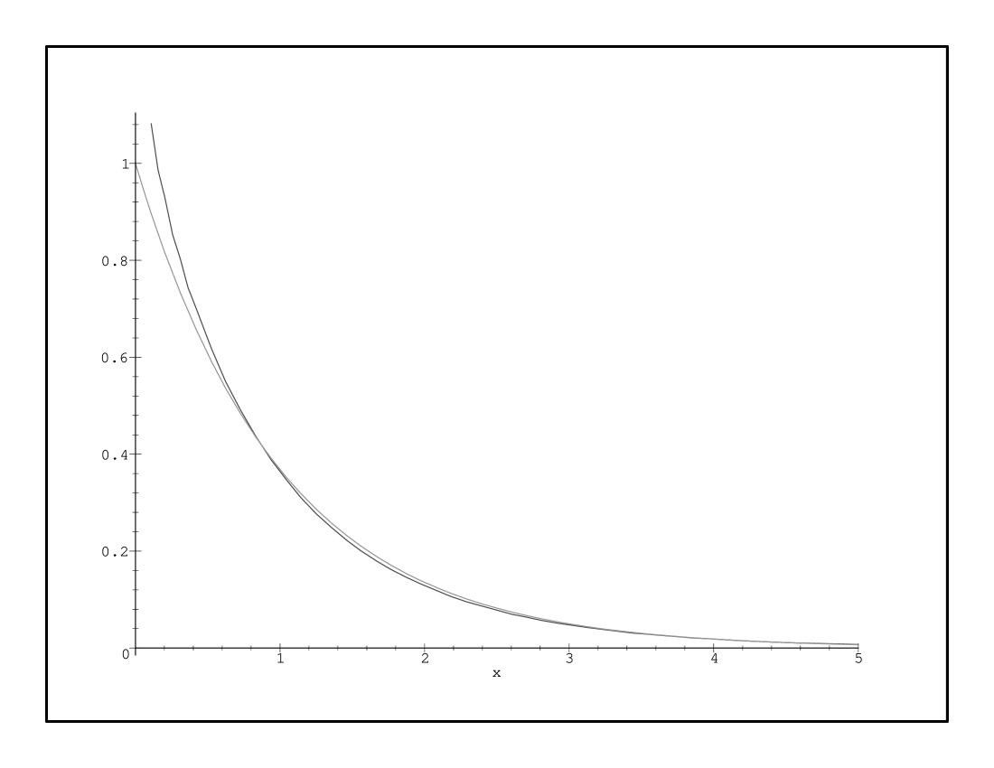
a)

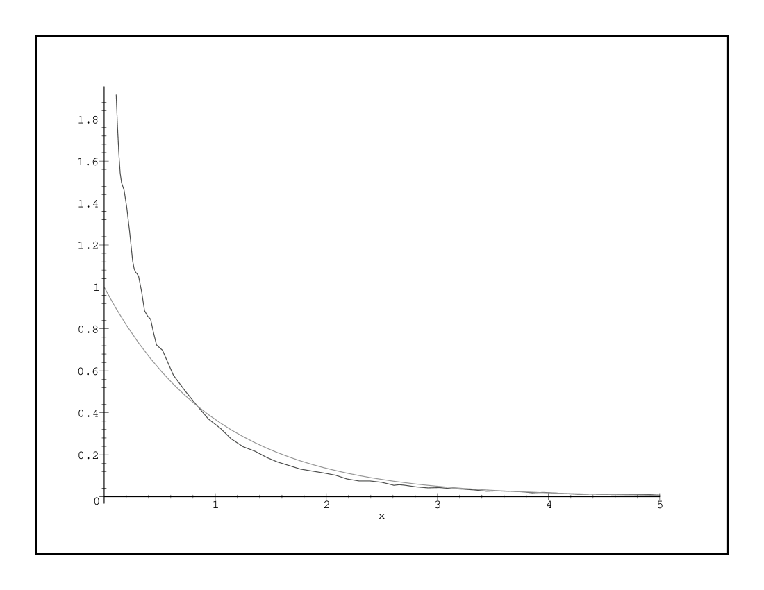
b)

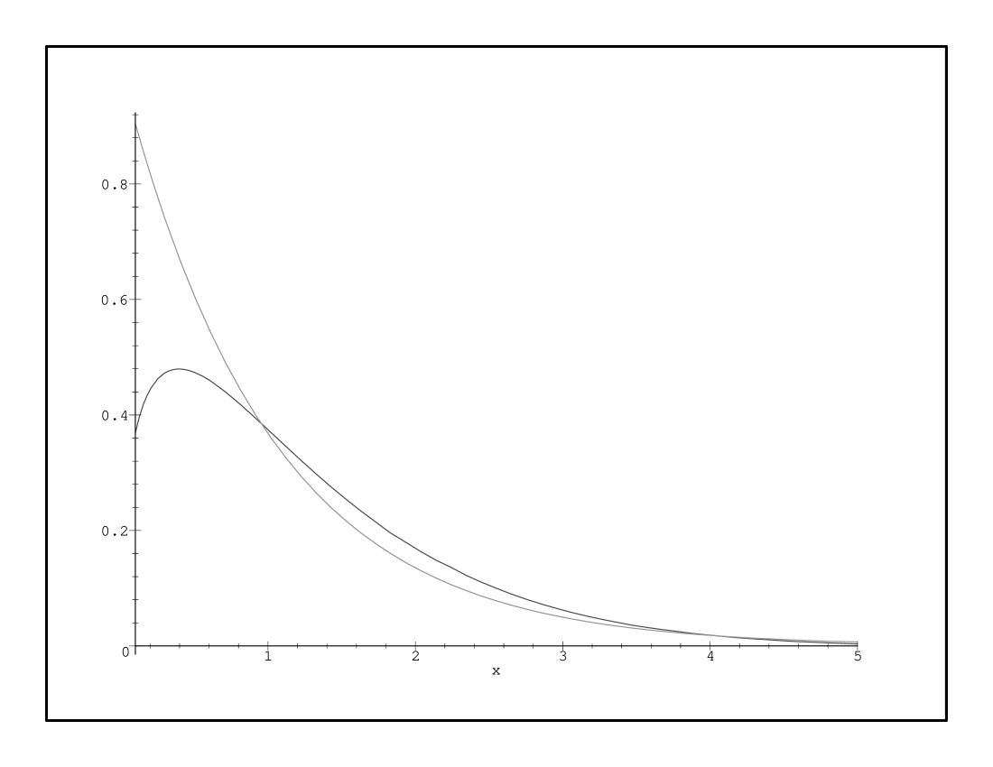
c)

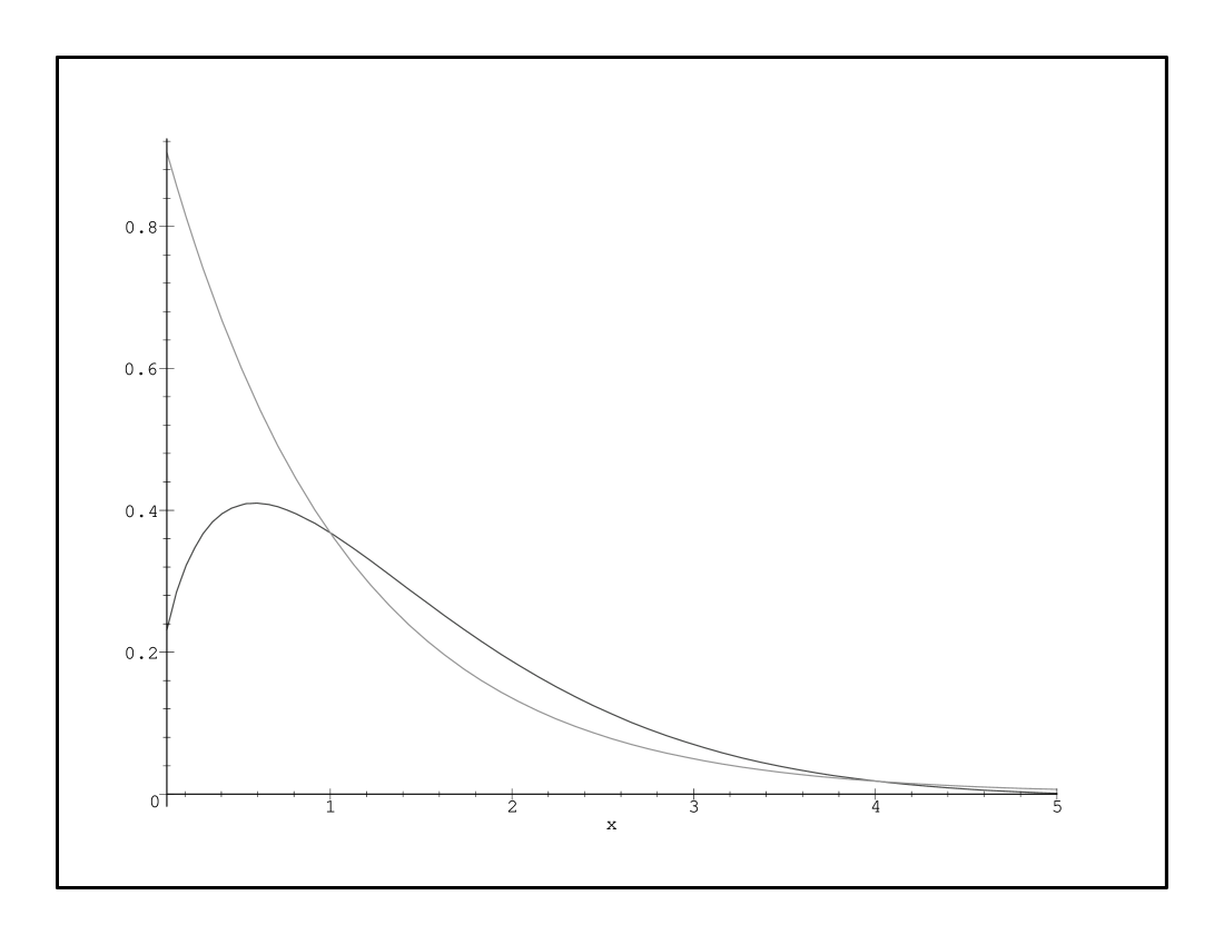
d)

Figure 1: Plots of Debye exponential factor $C_{D}(x)=\exp(-x/r_{D})$ with $r_{D}=1$ and the factors $y=C_{\alpha,0}(x)$ with $a_{0}=r^{-2}_{D}=1$ for the orders: a) $\alpha=1.9$, b) $\alpha=1.6$, c) $\alpha=2.5$, d) $\alpha=2.8$. Here $x=|{\bf r}|$ and we use $0<x<5$.

Using (Section 2.12.1 No.3. page 169. in [44]), we obtain the asymptotic ($|{\bf r}|\to 0$) in the form

$$C_{\alpha,0}(|{\bf r}|)\ \approx\ \frac{2^{2-\alpha}\,\Gamma((3-\alpha)/2)}{\sqrt{\pi}\,\Gamma(\alpha/2)}\frac{1}{|{\bf r}|^{2-\alpha}},\quad(1<\alpha<2),$$ (61)

$$C_{\alpha,0}(|{\bf r}|)\ \approx\ \frac{2^{2-\alpha}\,\Gamma((3-\alpha)/2)}{\sqrt{\pi}\,\Gamma(\alpha/2)}|{\bf r}|^{\alpha-2},\quad(2<\alpha<3),$$ (62)

$$C_{\alpha,0}(|{\bf r}|)\ \approx\ \frac{2\Gamma(3/\alpha)\,\Gamma(1-3/\alpha)}{\pi\,\alpha\,a^{1-3/\alpha}_{0}}\,|{\bf r}|,\quad(\alpha>3).$$ (63)

Note that asymptotic (61-62) for $1<\alpha<2$ and $2<\alpha<3$ does not depend on the parameter $a_{0}$. We point out that for $\alpha=2$, using (Equation (11) of Section 1.2. in the book [45]), we obtain Debye’s exponents $C_{2,0}(|{\bf r}|)=C_{D}(|{\bf r}|)$.

As a result, the electrostatic potential of the point charge in a media with this type of spatial dispersion will have the form

$$\Phi({\bf r})\ \approx\ \frac{Q}{4\pi\varepsilon_{0}}\frac{2^{2-\alpha}\,\Gamma((3-\alpha)/2)}{\sqrt{\pi}\,\Gamma(\alpha/2)}\,\frac{1}{|{\bf r}|^{3-\alpha}}\quad(1<\alpha<2,\quad 2<\alpha<3)$$ (64)

on small distances $|{\bf r}|\ll 1$. In the case $\alpha>3$, we have the constant value of the potential for $|{\bf r}|\ll 1$ given by

$$\Phi({\bf r})\ \approx\ \frac{1}{4\pi\varepsilon_{0}}\frac{Q}{R_{eff}},\quad(\alpha>3),$$ (65)

where $R_{eff}$ is an effective sphere radius that is equal to

$$R_{eff}=\frac{\pi\,\alpha\,a^{1-3/\alpha}_{0}}{2\Gamma(3/\alpha)\,\Gamma(1-3/\alpha)}.$$ (66)

Therefore, the electric field ${\bf E}$ is equal to zero at small distances $|{\bf r}|\ll 1$. It is well-known that the electric field inside a charged conducting sphere is zero, and that the potential remains constant at the value it reaches at the surface. Then the electric field of a point charge in the media with power-law of spatial dispersion with $\alpha>3$ is analogous to the field inside a conducting charged sphere of the radius $R_{eff}$, for small distances $|{\bf r}|\ll 1$.

The study of the asymptotic behavior of $C_{\alpha,2}(|{\bf r}|)$ for $|{\bf r}|\to\infty$ is an open question, although we have evidences to can suggest, as a conjecture, that its asymptotic behavior follow a power-law type also. Also from the corresponding plots, we can observe that the $C_{\alpha,2}(|{\bf r}|)$ decreases more slowly than Debye’s exponent $C_{D}(|{\bf r}|)$.

It is easy to proof that $C_{\alpha,2}(|{\bf r}|)$ has a maximum for the case $2<\alpha<3$ and the maximum does not exists for $1<\alpha<2$, while for the particular case $\alpha=2$ it is well-known that it is the classical exponential Debye’s screening.

2.3.2 Non-local deformation of Debye’s screening (the case $\alpha=2$)

Fractional model of non-local deformation of Debye’s screening in the media with spatial dispersion is described by equation (54) with $\alpha=2$, given by

$$-\Delta\Phi({\bf r})+a_{\beta}((-\Delta)^{\beta/2}\Phi)({\bf r})=\frac{1}{\varepsilon_{0}}\rho({\bf r}),$$ (67)

where $0<\beta<2$. The electrostatic potential of the point charge (22) has the following form

$$\Phi({\bf r})=\frac{1}{4\pi\varepsilon_{0}}\frac{Q}{|{\bf r}|}\,\cdot\,C_{2,\beta}(|{\bf r}|),$$ (68)

where the function

$$C_{2,\beta}(|{\bf r}|)=\frac{2}{\pi}\int^{\infty}_{0}\frac{\lambda\,\sin(\lambda|{\bf r}|)}{|\lambda|^{2}+a_{\beta}|\lambda|^{\beta}}\,d\lambda,$$ (69)

where $C_{2,\beta}(|{\bf r}|)$ describes the difference of Coulomb’s potential

In Figure 2 we present some plots of Debye exponential factor $C_{D}(|{\bf r}|)=\exp(-|{\bf r}|/r_{D})$ and factor $C_{2,\beta}(|{\bf r}|)$ for different orders of $1.5<\beta<2$ and $a_{\beta}=1$.

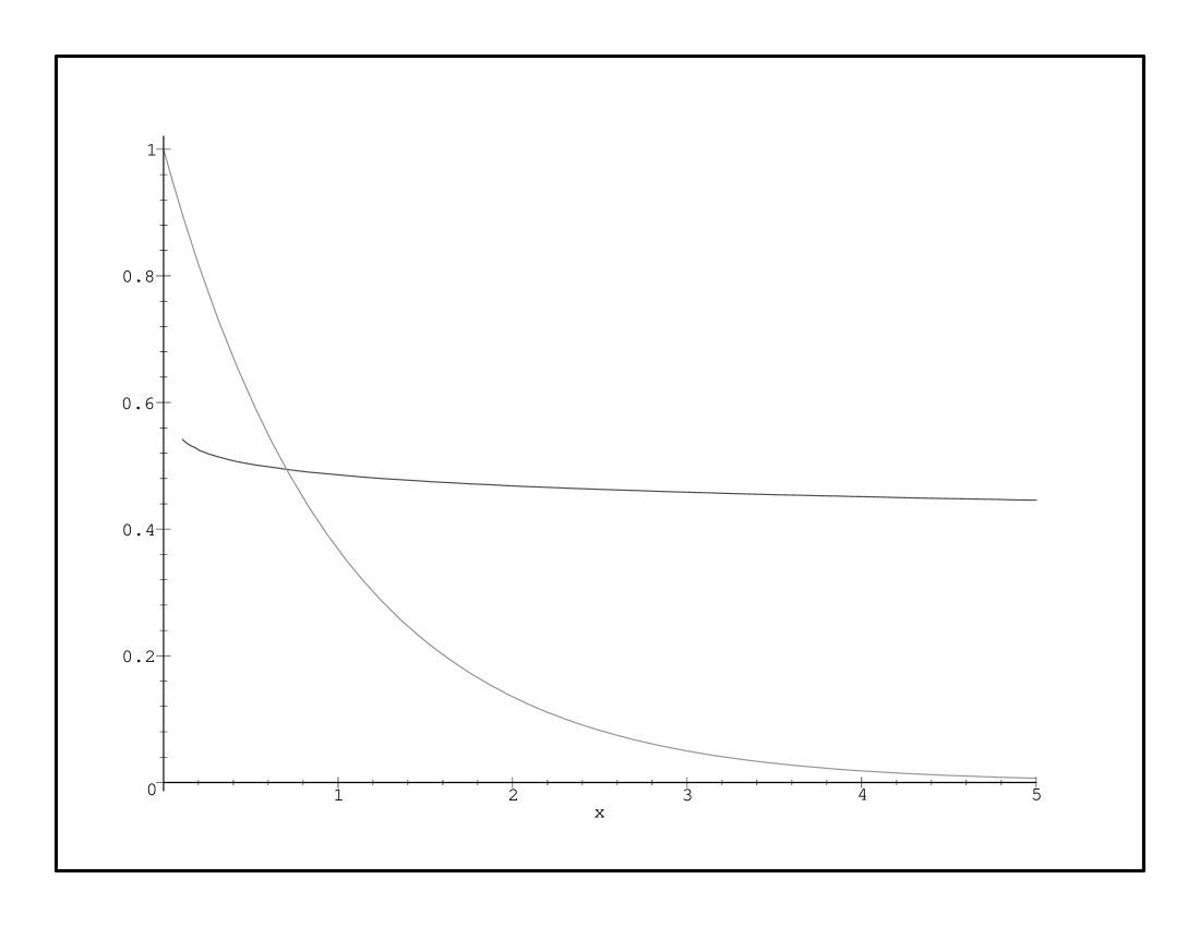
a)

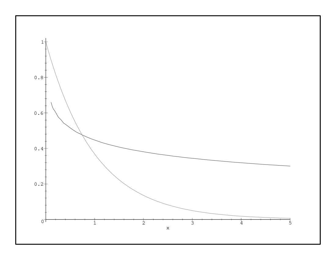
b)

c)

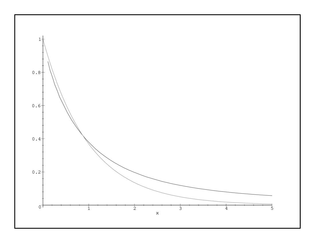
d)

Figure 2: Plots of Debye exponential factor $C_{D}(x)=\exp(-x/r_{D})$ with $r_{D}=1$ and the factors $y=C_{2,\beta}(x)$ with $a_{\beta}=1$ for the orders: a) $\beta=1.9$, b) $\beta=1.6$, c) $\beta=1.1$, d) $\beta=0.6$. Here $x=|{\bf r}|$ and we use $0<x<5$.

Using (Equation (1) of Section 2.3 in the book [45]), we obtain the following asymptotic behavior for $C_{2,\beta}(|{\bf r}|)$ with $\beta<2$, when $|{\bf r}|\to\infty$

$$C_{2,\beta}(|{\bf r}|)=\frac{2}{\pi}\int^{\infty}_{0}\frac{\lambda\sin(\lambda|{\bf r}|)}{\lambda^{2}+a_{\beta}\lambda^{\beta}}\,d\lambda\approx A_{0}(\beta)\frac{1}{|{\bf r}|^{2-\beta}}+\sum^{\infty}_{k=1}A_{k}(\beta)\frac{1}{|{\bf r}|^{(2-\beta)(k+1)}},$$ (70)

where

$$A_{0}(\beta)=\frac{2}{\pi a_{\beta}}\,\Gamma(2-\beta)\,\sin\left(\frac{\pi}{2}\beta\right),$$ (71)

$$A_{k}(\beta)=-\frac{2}{\pi a^{k+1}_{\beta}}\int^{\infty}_{0}z^{(2-\beta)(k+1)-1}\,\sin(z)\,dz.$$ (72)

As a result, we have that generalized non-local properties deforms Debye’s screening such that the exponential decay is replaced by the following generalized power-law

$$C_{2,\beta}(|{\bf r}|)\ \approx\ \frac{A_{0}}{|{\bf r}|^{2-\beta}}\quad(0<\beta<2).$$ (73)

On the other hand, the electrostatic potential of the point charge in the media with this type of spatial dispersion is given by

$$\Phi({\bf r})\ \approx\ \frac{A_{0}}{4\pi\varepsilon_{0}}\,\cdot\,\frac{Q}{|{\bf r}|^{3-\beta}}\quad(0<\beta<2)$$ (74)

on the long distance $|{\bf r}|\gg 1$.

2.3.3 Non-local deformation of Coulomb’s law and Debye’s screening (the case $\alpha\neq 2$ and $\beta>0$) together

The electrostatic potential for non-local fractional differential model that is described by equation (54) includes two parameters $(\alpha,\beta)$, where $\alpha>\beta>0$. In such model non-local properties deforms Coulomb’s law and Debye’s screening such that we have the following fractional power-law decay

$$C_{\alpha,\beta}(|{\bf r}|)\ \approx\ \frac{2\Gamma(2-\beta)\sin(\pi\beta/2)}{\pi a_{\beta}}\,\cdot\,\frac{1}{|{\bf r}|^{2-\beta}}\quad(|{\bf r}|\to\infty),$$ (75)

for $0<\beta<3$ and $\alpha>\beta$. Note that this asymptotic behavior $|{\bf r}|\to\infty$ does not depend on the parameter $\alpha$. The field on the long distances is determined only by term with $(-\Delta)^{\beta/2}$ ($\alpha>\beta$) that can be interpreted as a non-local deformation of Debye’s (second) term in equation (32).

The new type of behavior of the spatial-dispersion media with power-law non-locality is presented by power-law decreasing of the field at long distances instead of exponential decay.

The asymptotic behavior $C_{\alpha,\beta}(|{\bf r}|)$ for $|{\bf r}|\to 0$ is given by

$$C_{\alpha,\beta}(|{\bf r}|)\ \approx\ \frac{2^{2-\alpha}\,\Gamma((3-\alpha)/2)}{\sqrt{\pi}\,\Gamma(\alpha/2)}\,\cdot\,\frac{1}{|{\bf r}|^{2-\alpha}},\quad(1<\alpha<2),$$ (76)

$$C_{\alpha,\beta}(|{\bf r}|)\ \approx\ \frac{2^{2-\alpha}\,\Gamma((3-\alpha)/2)}{\sqrt{\pi}\,\Gamma(\alpha/2)}\,\cdot\,|{\bf r}|^{\alpha-2},\quad(2<\alpha<3),$$ (77)

$$C_{\alpha,\beta}(|{\bf r}|)\ \approx\ \frac{2}{\alpha\,a^{1-3/\alpha}_{\beta}\,\sin(3\pi/\alpha)}\,\cdot\,|{\bf r}|,\quad(\alpha>3),$$ (78)

where we use Euler’s reflection formula for Gamma function. Note that the above asymptotic behavior does not depend on the parameter $\beta$, and relations (76-77) does not depend on $a_{\beta}$. The field on the short distances is determined only by term with $(-\Delta)^{\alpha/2}$ ($\alpha>\beta$) that can be considered as a non-local deformation of Coulomb’s (first) term in equation (32).

On the other hand, it is remarkable that exist a maximum for the factor $C_{\alpha,\beta}(|{\bf r}|)$ in the case $0<\beta<2<\alpha$.

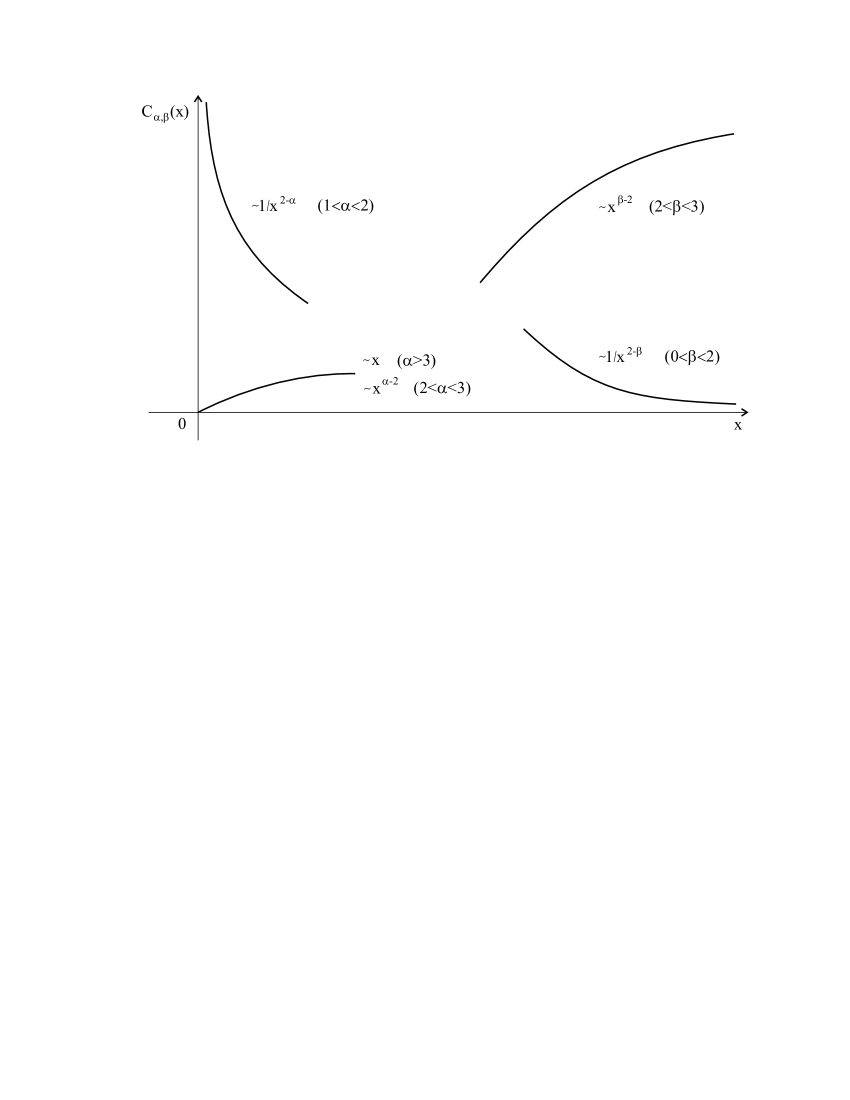
Figure 3: Plots of general asymptotic behaviors of the factor $y=C_{\alpha,\beta}(x)$.

3 Fractional Weak Spatial Dispersion

Here we introduce a generalization of well-known weak spatial dispersion for the power-law type of non-locality of the media [24, 25, 26, 27, 28, 29].

3.1 Weak Spatial Dispersion

Let us give an short description of weak spatial dispersion in the plasma-like media (for details see, for instance, [24, 25, 26]).

Spatial dispersion in electrodynamics is called to the dependence of the tensor of the absolute permittivity of the medium on the wave vector [24, 25, 26]. It is well-known that this dependence leads to a number of phenomena, for example the rotation of the plane of polarization, anisotropy of cubic crystals and other [27, 28, 29, 30, 31, 32, 33, 34, 35, 36, 37, 38].

The spatial dispersion is caused by non-local connection between the electric induction ${\bf D}$ and the electric field ${\bf E}$. Vector ${\bf D}$ at any point ${\bf r}$ of the medium is not uniquely defined by the values of ${\bf E}$ at this point. It also depends on the values of ${\bf E}$ at neighboring points ${\bf r}^{\prime}$, located near the point ${\bf r}$.

Non-local connection between ${\bf D}$ and ${\bf E}$ can be understood on the basis of qualitative analysis of a simple model of the crystal. In this model the particles of the crystal lattice (atoms, molecules, ions) oscillate about their equilibrium positions and interact with each other. The equations of oscillations of the crystal lattice particles with the local (nearest-neighbor) interaction gives the partial differential equation of integer orders in the continuous limits [40, 41]. Note that non-local (long-range) interactions in the crystal lattice in the continuous limit can give a fractional partial differential equations [40, 41]. It was shown in [40, 41] that the equations of oscillations of crystal lattice with long-range interaction are mapped into the continuum equation with the Riesz fractional derivative.

The electric field of the light wave moves charges from their equilibrium positions at a given point ${\bf r}$, which causes an additional shift of the charges in neighboring and more distant points ${\bf r}^{\prime}$ in some neighborhood. Therefore, the polarization of the medium, and hence the field ${\bf D}$ depend on the values of the electric fields ${\bf E}$ not only in a selected point, but also in its neighborhood. This applies not only to the crystals, but also to isotropic media consisting of asymmetric molecules and plasma-like media [24, 25, 26].

The size of the area in which the kernel $\hat{\varepsilon}_{ij}({\bf r})$ of integral equation (12) is significantly determined by the characteristic lengths of interaction $R_{0}$. For different media these lengths can vary widely. The size of the area of the mutual influence $R_{0}$ are usually on the order of the lattice constant or the size of the molecules (for dielectric media). Wavelength of light $\lambda$ is several orders larger than the size of this region, so for a region of size $R_{0}$ value of the electromagnetic field of light wave does not change. By other words, in the dielectric media for optical wavelength $\lambda$ usually holds $kR_{0}\sim R_{0}/\lambda\sim 10^{-3}\ll 1$. In such media the spatial dispersion is weak [24, 25, 27, 38]. To analyze it is enough to know the dependence of the tensor $\varepsilon_{ij}({\bf k})$ only for small values ${\bf k}$ and we can replace the function by the Taylor polynomial

$$\varepsilon_{ij}({\bf k})=\varepsilon_{ij}+\gamma_{ijl}k_{l}+\delta_{ijlm}k_{l}k_{m}+...\quad.$$ (79)

Here we neglect the frequency dispersion, and so the tensors $\varepsilon_{ij}$, $\gamma_{ijl}$, $\delta_{ijlm}$ do not depend on the frequency $\omega$.

The tensors in (79) are simplified for crystals with high symmetry [27]. For an isotropic linear medium, we can use

$$\varepsilon_{\parallel}(|{\bf k}|)=\varepsilon+\gamma|{\bf k}|+\delta|{\bf k}|^{2}+...\quad.$$ (80)

In order to explain the natural optical activity (for example, optical rotation, gyrotropy) is sufficient to consider the linear dependence on ${\bf k}$ in (79) and (80). For non-gyrotropic crystals it is necessary to take into account the terms quadratic in ${\bf k}$.

For power-like type of non-locality we should use fractional generalizations of the Taylor formula (see Appendix 2).

3.2 Fractional Taylor series approach

The weak spatial dispersion in the media with power-law type of non-locality cannot be describes by the usual Taylor approximation. The fractional Taylor series is very useful for approximating non-integer power-law functions [39]. To illustrate this point, we consider the non-linear power-law function

$$\varepsilon_{\parallel}(|{\bf k}|)=a_{\alpha}|{\bf k}|^{\alpha}+a_{0}.$$ (81)

If we use the usual Taylor series for the function (81) then we have infinite series.

For fractional Taylor formula of Caputo type (see Appendix 2), we need the following known property of the fractional Caputo derivative ${}_{a}^{C}D^{\alpha}_{k}$ (see, for instance, [6])

$$_{a}^{C}D^{\alpha}_{k}(k-a)^{\beta}=\frac{\Gamma(\beta+1)}{\Gamma(\beta-\alpha+1)}\,(k-a)^{\beta-\alpha},\quad(x>a,\ \alpha>0,\ \beta>0),$$ (82)

where $k=|\bf{k}|$. In particular, if $\beta=\alpha$, then

$$\,{}_{a}^{C}D^{\alpha}_{k}(k-a)^{\alpha}=\Gamma(\alpha+1),\quad(\,_{a}^{C}D^{\alpha}_{k})^{n}(k-a)^{\alpha}=0.$$ (83)

Therefore

$$(\,^{C}D^{\alpha}\varepsilon_{\parallel})(0)=\Gamma(\alpha+1),$$

while, the higher order Caputo fractional derivatives of $\varepsilon_{\parallel}(|{\bf k}|)$, given in (81), are all zero. Hence, the fractional Taylor series approximation of such function is exact. Note that the order of non-linearity of $\varepsilon_{\parallel}(|{\bf k}|)$ is equal to the order of the Taylor series approximation.

3.3 Weak spatial dispersion of power-law types

We consider such properties of the media with weak spatial dispersion that is described by the non-integer power-law type of functions $\varepsilon_{\parallel}(|{\bf k}|)$. The fractional differential model is used to describe a new possible type of behavior of complex media with power-law non-locality.

The weak spatial dispersion (and the permittivity) will be called $\alpha$-type, if the function $\varepsilon_{\parallel}(|{\bf k}|)$ satisfies the condition

$$\lim_{|{\bf k}|\to 0}\frac{\varepsilon_{\parallel}(|{\bf k}|)-\varepsilon_{\parallel}(0)}{\varepsilon_{0}\,|{\bf k}|^{\alpha}}=a_{\alpha},$$ (84)

where $\alpha>0$ and $0<|a_{\alpha}|<\infty$. Here the constant $\varepsilon_{0}$ is the vacuum permittivity ($\varepsilon_{0}\approx 8.854\,10^{-12}F\cdot m^{-1}$).

The weak spatial dispersion (the permittivity) will be called $(\alpha,\beta)$-type, if the function $\varepsilon_{\parallel}(|{\bf k}|)$ satisfies the conditions (84) and

$$\lim_{|{\bf k}|\to 0}\frac{\varepsilon_{\parallel}(|{\bf k}|)-\varepsilon_{\parallel}(0)-a_{\alpha}\varepsilon_{0}\,|{\bf k}|^{\alpha}}{\varepsilon_{0}|{\bf k}|^{\beta}}=a_{\beta},$$ (85)

where $\beta>\alpha>0$ and $0<|a_{\beta}|<\infty$.

Note that these definitions are similar to definitions of non-local alpha-interactions between particles of crystal lattice (see Section 8.6 in [19] and [40, 41]) that give continuous medium equations with fractional derivatives with respect to coordinates.

For the weak spatial dispersion of the $(\alpha,\beta)$-type, the permittivity can be represented in the form

$$\varepsilon_{\parallel}(|{\bf k}|)=\varepsilon_{0}(\varepsilon+a_{\alpha}|{\bf k}|^{\alpha}+a_{\beta}|{\bf k}|^{\beta})+R_{\alpha,\beta}(|{\bf k}|),$$ (86)

where $\varepsilon=\varepsilon_{\parallel}(0)/\varepsilon_{0}$ can be considered as the relative permittivity of material, and

$$\lim_{|{\bf k}|\to 0}\frac{R_{\alpha,\beta}(|{\bf k}|)}{|{\bf k}|^{\beta}}=0.$$ (87)

As a result, we can use the following approximation for weak spatial dispersion

$$\varepsilon_{\parallel}(|{\bf k}|)/\varepsilon_{0}\approx\varepsilon+a_{\alpha}|{\bf k}|^{\alpha}+a_{\beta}|{\bf k}|^{\beta}.$$ (88)

If $\alpha=1$ and $\beta=2$, we can use the usual Taylor formula. In this case we have the well-known case of the weak spatial dispersion [27, 28, 29, 30, 31, 32, 33, 34, 35, 36, 37, 38] In general, we should use a fractional generalization of the Taylor series (see Appendix 2). If the orders of the fractional Taylor series approximation will be correlated with the type of weak spatial dispersion, then the fractional Taylor series approximation of $\varepsilon_{\parallel}(|{\bf k}|)$ will be exact. In the general case, $\beta\neq\alpha$, where $0<\beta-\alpha<1$, we can use the fractional Taylor formula in the Dzherbashyan-Nersesian form (see Appendix 2). For the special cases $\beta=2\alpha$, where $\alpha<1$ and/or $\beta=\alpha+1$, we could use other kind of the fractional Taylor formulas. In the fractional cases new types of physical effects may exist.

3.4 Fractional differential equation for electrostatic potential

We can consider a weak spatial dispersion of the power-law $(\alpha,\beta)$-type. Then substituting (88) into (21), we obtain

$$\Bigl{(}\varepsilon|{\bf k}|^{2}+a_{\alpha}|{\bf k}|^{\alpha+2}+a_{\beta}|{\bf k}|^{\beta+2}\Bigr{)}\,\Phi_{\bf k}=\frac{1}{\varepsilon_{0}}\rho_{\bf k},$$ (89)

where $\varepsilon=\varepsilon_{\parallel}(0)\varepsilon_{0}$ and $\beta>\alpha>0$. The inverse Fourier transform of (89) gives

$$a_{\beta}((-\Delta)^{(\beta+2)/2}\Phi)({\bf r})+a_{\alpha}((-\Delta)^{(\alpha+2)/2}\Phi)({\bf r})-\varepsilon\Delta\Phi({\bf r})=\frac{1}{\varepsilon_{0}}\rho({\bf r}).$$ (90)

This fractional differential equation describes a weak spatial dispersion of the $(\alpha,\beta)$-type.

Equation (90) has the following particular solution

$$\Phi({\bf r})=\frac{1}{\varepsilon_{0}}\int_{\mathbb{R}^{3}}G_{2,\alpha,\beta}({\bf r}-{\bf r}^{\prime})\,\rho({\bf r}^{\prime})\,d^{3}{\bf r}^{\prime},$$ (91)

where $G_{2,\alpha,\beta}$ is the Green function of the form

$$G_{2,\alpha,\beta}({\bf r})=\frac{|{\bf r}|^{-1/2}}{(2\pi)^{3/2}}\int^{\infty}_{0}\left(a_{\alpha}|\lambda|^{\alpha+2}+a_{\beta}|\lambda|^{\beta+2}+\varepsilon|\lambda|^{2}\right)^{-1}\lambda^{3/2}\,J_{1/2}(\lambda|{\bf r}|)\,d\lambda.$$ (92)

Therefore, the electrostatic potential of the point charge (22) for this case is given by

$$\Phi({\bf r})=\frac{1}{4\pi\varepsilon_{0}}\frac{Q}{|{\bf r}|}\cdot C_{2,\alpha,\beta}(|{\bf r}|),$$ (93)

where $0<\alpha<\beta$, and the function

$$C_{2,\alpha,\beta}(|{\bf r}|)=\frac{2}{\pi}\,\int^{\infty}_{0}\frac{\lambda\,\sin(\lambda|{\bf r}|)}{a_{\alpha}|\lambda|^{\alpha+2}+a_{\beta}|\lambda|^{\beta+2}+\varepsilon|\lambda|^{2}}\,d\lambda$$ (94)

describes the difference between such generalized potential and Coulomb’s potential.

For the weak spatial dispersion of the $\alpha$-type, we have

$$a_{\alpha}((-\Delta)^{(\alpha+2)/2}\Phi)({\bf r})-\varepsilon\Delta\Phi({\bf r})=\frac{1}{\varepsilon_{0}}\rho({\bf r}).$$ (95)

This equation is a special case of equation (90), where $a_{\beta}=0$. Then, the electrostatic potential of the point charge has form

$$\Phi({\bf r})=\frac{1}{4\pi\varepsilon_{0}}\frac{Q}{|{\bf r}|}\ \cdot C_{2,\alpha,0}(|{\bf r}|),$$ (96)

where $0<\alpha<\beta$, and

$$C_{2,\alpha,0}(|{\bf r}|)=\frac{2}{\pi}\,\int^{\infty}_{0}\frac{\lambda\,\sin(\lambda|{\bf r}|)}{a_{\alpha}|\lambda|^{\alpha+2}+\varepsilon|\lambda|^{2}}\,d\lambda.$$ (97)

This case is described by the fractional differential model introduced in Section 3 for the case of the order of Riesz fractional derivative is $\alpha+2>2$.

To describe properties of electric field of the point charge in the media with weak spatial dispersion, we consider properties of the function

$$C_{2,\alpha,\beta}(|{\bf r}|)=\frac{2}{\pi}\,\int^{\infty}_{0}\frac{\lambda\,\sin(\lambda|{\bf r}|)}{a_{\beta}|\lambda|^{\beta+2}+a_{\alpha}|\lambda|^{\alpha+2}+\varepsilon|\lambda|^{2}}\,d\lambda,$$ (98)

where $\beta>\alpha$.

Using the values for the sine integral $Si(x)$ for the infinite limit

$$\int^{\infty}_{0}\frac{\sin(z)}{z}=\frac{\pi}{2},$$ (99)

and the equation for the integral transform (Section 2.3, equation (1) in [45]) of the form

$$\int^{\infty}_{0}z^{\alpha-1}\,\sin(z)=\Gamma(\alpha)\sin\left(\frac{\pi\beta}{2}\right),\quad(-1<\alpha<1),$$ (100)

we obtain the asymptotic for the function $C_{2,\alpha,\beta}(|{\bf r}|)$ of the form

$$C_{2,\alpha,\beta}(|{\bf r}|)\approx\frac{2}{\pi\varepsilon}\,\Bigl{(}\frac{\pi}{2}-\frac{1}{|{\bf r}|^{\alpha}}\frac{a_{\alpha}}{\varepsilon}\,\Gamma(\alpha)\,\sin\left(\frac{\pi\alpha}{2}\right)-\frac{1}{|{\bf r}|^{\beta}}\frac{a_{\beta}}{\varepsilon}\,\Gamma(\beta)\,\sin\left(\frac{\pi\beta}{2}\right)\Bigr{)}.$$ (101)

It allows us to obtain the asymptotic behavior of the electrostatic potential

$$\Phi({\bf r})\ \approx\ \frac{Q}{4\pi\varepsilon\varepsilon_{0}}\frac{1}{|{\bf r}|}-\frac{a_{\alpha}Q}{4\pi\varepsilon^{2}\varepsilon_{0}}\frac{2\Gamma(\alpha)\,\sin(\pi\alpha/2)}{\pi}\frac{1}{|{\bf r}|^{\alpha+1}}-\frac{a_{\beta}Q}{4\pi\varepsilon^{2}\varepsilon_{0}}\frac{2\Gamma(\beta)\,\sin(\pi\beta/2)}{\pi}\frac{1}{|{\bf r}|^{\beta+1}},$$ (102)

where $0<\alpha<\beta<1$.

The parameter $\varepsilon$ is interpreted as a relative permittivity of the media. It is well known that far from the electric dipole the electrostatic potential of its electric field decreases with distance $|{\bf r}|$, as $|{\bf r}|^{-2}$ (see Section 40 in [46]), that is faster than the point charge potential ($\Phi({\bf r})\sim|{\bf r}|^{-1}$).

The first term in (102) describes the well-known Coulomb’s field. The second and third terms in (102) look like changed dipole electrostatic field that for integer case ($\alpha=1$) has the from $\Phi({\bf r})=d\cos\theta/(4\pi\varepsilon_{0}\,|{\bf r}|^{2})$, where $d=|{\bf d}|$, and ${\bf d}$ is the (vector) dipole moment, and $\theta$ is an angle between the vectors ${\bf d}$ and ${\bf r}$ (see Section 40 in [46]). We can consider the effective values

$$d_{eff}(\alpha)=\frac{2\Gamma(\alpha)a_{\alpha}Q}{\pi\varepsilon^{2}},\quad\theta_{eff}=\frac{\pi}{2}(1-\alpha)$$ (103)

for non-integer values of $\alpha$. The second and third terms in equation (102) can be interpreted as a generalized dipole fields of power-law type with the non-integer orders $\alpha$ and $\beta$, and these terms are represented as

$$\Phi_{eff}({\bf r})=-\frac{d_{eff}(\alpha)\cos\theta_{eff}(\alpha)}{4\pi\varepsilon_{0}\,|{\bf r}|^{\alpha+1}}-\frac{d_{eff}(\beta)\cos\theta_{eff}(\beta)}{4\pi\varepsilon_{0}\,|{\bf r}|^{\beta+1}},$$ (104)

where $0<\alpha<\beta<1$.

In Figure 4 present some plots (see Figure 3) of Coulomb’s electrostatic potentials $\Phi(|{\bf r}|)=(1/4\pi\varepsilon_{0})|{\bf r}|^{-1}$ and the potential with factor $C_{\beta,\alpha,2}(|{\bf r}|)$ for different orders of $0<\alpha<\beta<2$, where $a_{\beta}=a_{\alpha}=\varepsilon=1$.

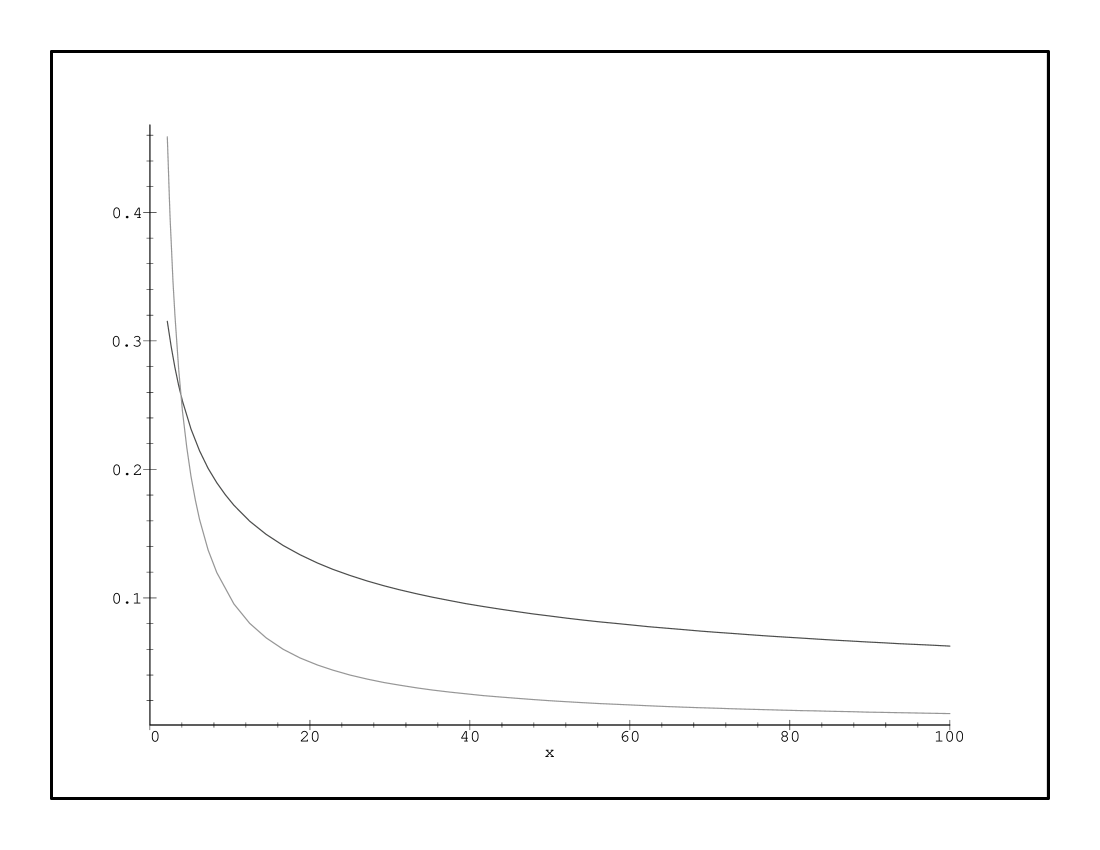
a)

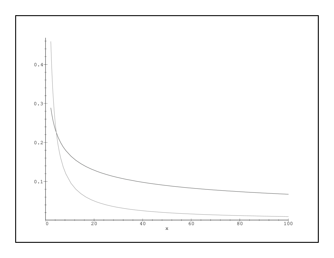
b)

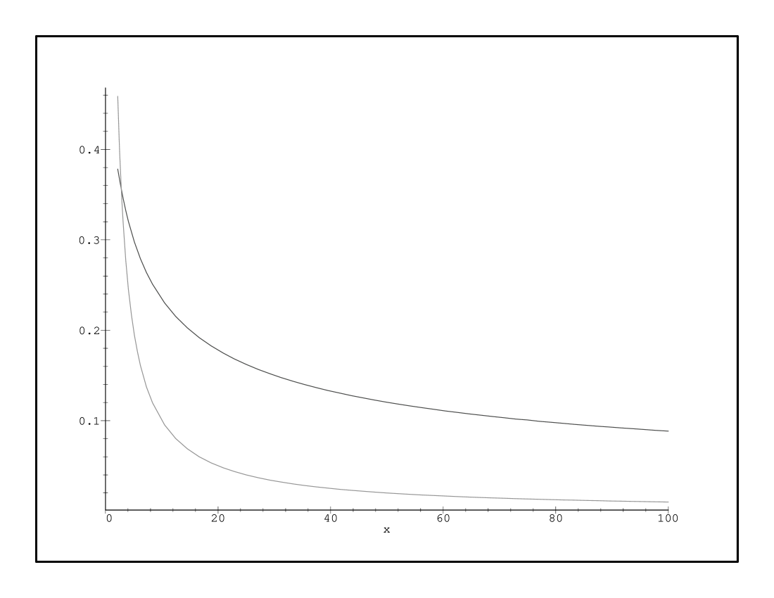
c)

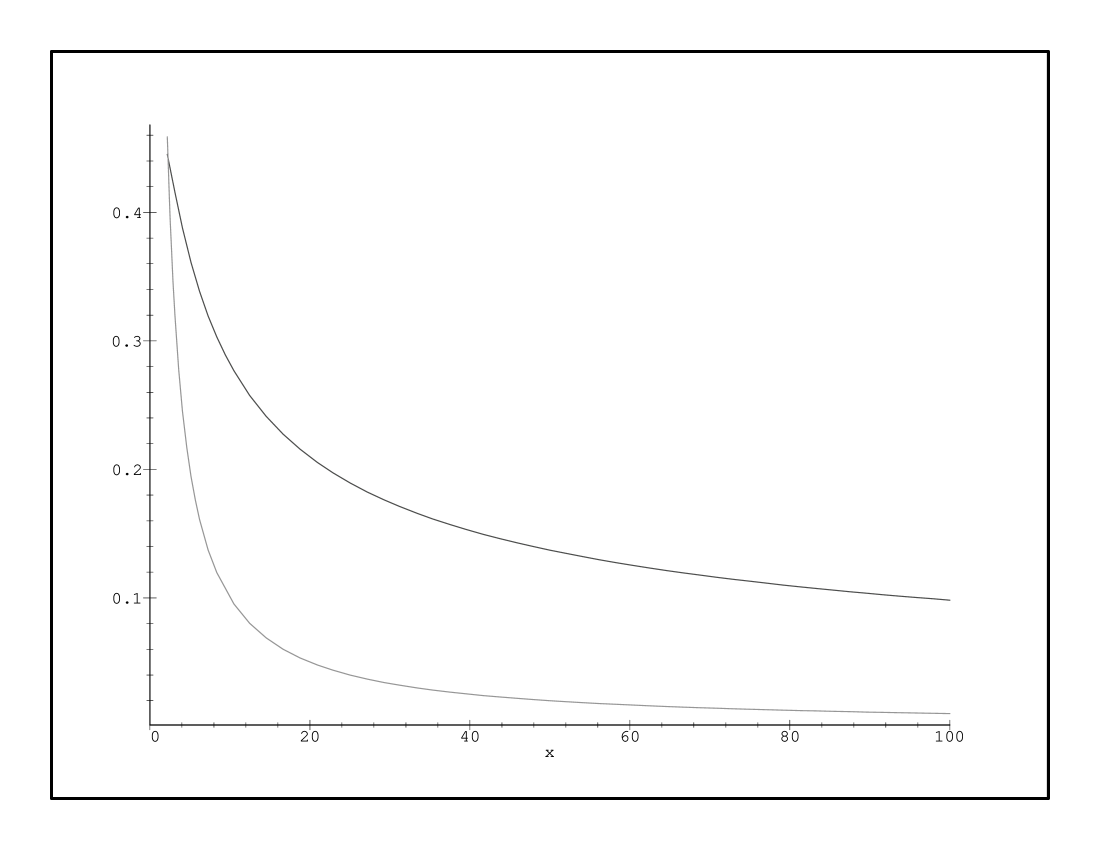
d)

Figure 4: Plots of Coulomb’s electrostatic potential $\Phi(x)=x^{-1}$ and the electrostatic potentials $y=x^{-1}\cdot C_{2,\alpha,\beta}(x)$ (the weak spatial dispersion case) with $a_{\beta}=a_{\alpha}=\varepsilon=1$ for the orders: a) $\alpha=0.1$ and $\beta=1.1$, b)$\alpha=0.2$ and $\beta=0.4$, c) $\alpha=0.4$ and $\beta=1.4$, d) $\alpha=0.8$ and $\beta=1.8$. Here $x=|{\bf r}|$ and we use $0<x<100$. The asymptotic behavior for long distances is defined by $\beta$ only.

From the plots (see Figure 4) it is easy to see that far from the point charge in the media with weak spatial dispersion the electrostatic potential decreases with distance $|{\bf r}|$ more slowly (102) than the potential of the point charge potential ($\Phi({\bf r})\sim|{\bf r}|^{-1}$).

4 Conclusion

We consider fractional power-law type generalizations of permittivity, and generalizations of the correspondent equations for electrostatic potential $\Phi({\bf r})$ by involving the fractional generalization of the Laplacian [42, 43, 5, 6]. The simplest power-law forms of the longitudinal permittivity $\varepsilon_{\parallel}(|{\bf k}|)=\varepsilon_{0}\Bigl{(}|{\bf k}|^{\alpha-2}+r^{-2}_{D}\,|{\bf k}|^{\beta-2}\Bigr{)}$ are suggested. The parameter $\alpha$ characterizes the deviation from Coulomb’s law due to non-local properties of the medium. The parameter $\beta$ characterizes the deviation from Debye’s screening due to non-integer power-law type of non-locality in the medium. The correspondent equation (35) for electrostatic potential $\Phi({\bf r})$ that has the form $((-\Delta)^{\alpha/2}\Phi)({\bf r})+r^{-2}_{D}((-\Delta)^{\beta/2}\Phi)({\bf r})=\varepsilon^{-1}_{0}\rho({\bf r})$, contains $(-\Delta)^{\alpha/2}$ and $(-\Delta)^{\beta/2}$ are the Riesz fractional Laplacian [42, 43, 5, 6], and ${\bf r}$ and $r_{D}$ are dimensionless variables.

To the mentioned model can be find a explicit solution in terms of a Green type function. Also we will describe analytic solutions of the fractional differential equations (35) for electrostatic potentials. The electrostatic potential of the point charge has form $\Phi({\bf r})=Q/(4\pi\varepsilon_{0}|{\bf r}|)\cdot C_{\alpha,\beta}(|{\bf r}|)$, where $C_{\alpha,\beta}(|{\bf r}|)$ is defined by (58) describes the differences of Coulomb’s potential and Debye’s screening. Using the analytic solutions of the fractional differential equations for electrostatic potentials, we describe the asymptotic behaviors of the electrostatic potential. The new type of behavior of the spatial-dispersion media with power-law non-locality is presented by power-law decreasing of the field at long distances instead of exponential decay.

In order to describe the properties of deviations separately, we consider the following special cases of the proposed model:

1) Fractional model of non-local deformation of Coulomb’s law in the media with spatial dispersion that corresponds to the case $\beta=0$ and $\alpha\neq 2$, $\alpha>1$. This model allows us to describe a possible deviation from Coulomb’s law in the media with nonlocal properties defined by power-law type of spatial dispersion.

The electrostatic potential of the point charge in a media with this type of spatial dispersion has the form $\Phi({\bf r})\ \sim\ |{\bf r}|^{\alpha-3}$ for $1<\alpha<2$ and $2<\alpha<3$ on small distances $|{\bf r}|\to 0$. In the case $\alpha>3$, we have the constant value of the potential for $|{\bf r}|\to 0$. Therefore the electric field ${\bf E}$ of a point charge in the media with power-law type of spatial dispersion with $\alpha>3$ is equal to zero at small distances $|{\bf r}|\to 0$ that is analogous to the well-known case of the field inside a conducting charged sphere of the radius $R_{eff}$, for small distances. The asymptotic behavior of potential for $|{\bf r}|\to\infty$ follow a power-law type also by our assumption. From the corresponding plots, we observe that the $C_{\alpha,2}(|{\bf r}|)$ decreases more slowly than Debye’s exponent $C_{D}(|{\bf r}|)$. The function $C_{\alpha,2}(|{\bf r}|)$ has a maximum for the case $2<\alpha<3$ and the maximum does not exists for $1<\alpha<2$, while for the particular case $\alpha=2$ it is well-known that it is the classical exponential Debye’s screening.

2) Fractional model of non-local deformation of Debye’s screening in the media with spatial dispersion is defined by $\alpha=2$ and $0<\beta<2$. Such model allows us to describe a possible deviation from Debye’s screening by non-local properties of the plasma-like media with the generalized power-law type of spatial dispersion.

The generalized non-local properties deforms Debye’s screening such that the exponential decay is replaced by the fractional power-law, and the electrostatic potential of the point charge in the media with this type of spatial dispersion is given by $\Phi({\bf r})\ \sim\ |{\bf r}|^{\beta-3}$ for $0<\beta<2$ on the long distance $|{\bf r}|\to\infty$.

3) Fractional non-local model that is described by equation (54) includes two parameters $(\alpha,\beta)$, where $\alpha>\beta>0$ such that $\alpha\neq 2$. In such model non-local properties deforms Coulomb’s law and Debye’s screening such that we have the fractional power-law decay for $0<\beta<3$ and $\alpha>\beta$. The asymptotic behavior $|{\bf r}|\to\infty$ does not depend on the parameter $\alpha$. The field on the long distances is determined only by term with $(-\Delta)^{\beta/2}$ that can be interpreted as a non-local deformation of Debye’s term. It is remarkable that exist a maximum for the factor $C_{\alpha,\beta}(|{\bf r}|)$ in the case $0<\beta<2<\alpha$.

The asymptotic behavior for $|{\bf r}|\to 0$ is given by $\Phi({\bf r})\ \sim\ |{\bf r}|^{\alpha-3}$ for $1<\alpha<2$ and $2<\alpha<3$, and $\Phi({\bf r})$ is a constant for $\alpha>3$. Note that the above asymptotic behavior does not depend on the parameters $\beta$ and $r^{-2}_{D}$. The field on the short distances is determined only by term with $(-\Delta)^{\alpha/2}$, that can be considered as a non-local deformation of Coulomb’s term.

We also consider weak spatial dispersion in the media with fractional power-law type of non-locality. In general, it cannot be describes by the usual Taylor approximation. The fractional Taylor series is very useful for approximating non-integer power-law functions. The media with spatial dispersion is described by the non-integer power-law type of functions $\varepsilon_{\parallel}(|{\bf k}|)$. Using fractional generalization of the Taylor series (see Appendix 2), we get approximations of the form $\varepsilon_{\parallel}(|{\bf k}|)/\varepsilon_{0}\approx\varepsilon+a_{\alpha}|{\bf k}|^{\alpha}+a_{\beta}|{\bf k}|^{\beta}$ for such type of media. If $\alpha=1$ and $\beta=2$, we have the usual Taylor formula, and the well-known case of the weak spatial dispersion [27, 28, 29, 30, 31, 32, 33, 34, 35, 36, 37, 38]. In general, we should use a fractional generalization of the Taylor series. If the orders of the fractional Taylor series approximation will be correlated with the type of weak spatial dispersion, then the fractional Taylor series approximation for $\varepsilon_{\parallel}(|{\bf k}|)$ will be exact.

These fractional weak spatial dispersions is described by equation of the form $a_{\beta}((-\Delta)^{(\beta+2)/2}\Phi)({\bf r})+a_{\alpha}((-\Delta)^{(\alpha+2)/2}\Phi)({\bf r})-\varepsilon\Delta\Phi({\bf r})=\frac{1}{\varepsilon_{0}}\rho({\bf r})$. To this fractional differential equation we can be find a explicit solution in terms of a Green type function. Also we describe analytic solutions of the fractional differential equations for electrostatic potentials. It allows us to obtain the asymptotic behavior of the electrostatic potential of the form $\Phi({\bf r})\ \approx\ \Phi_{Coulomb}({\bf r})+\Phi^{(\alpha)}_{eff,dipole}({\bf r})+\Phi^{(\beta)}_{eff,dipole}({\bf r})$, where $0<\alpha<\beta<1$. The first term describes Coulomb’s field. The second and third terms are interpreted as electrostatic fields generalized of changed dipoles of power-law type with the non-integer orders $\alpha$ and $\beta$, which have the form $\Phi^{(\alpha)}_{eff}({\bf r})=-{d_{eff}(\alpha)\cos\theta_{eff}(\alpha)}/(4\pi\varepsilon_{0}\,|{\bf r}|^{\alpha+1})$, where $0<\alpha<\beta<1$, $d_{eff}$ is the effective dipole moment, and $\theta$ is an effective angle. For integer case ($\alpha=1$) we have the usual from $\Phi({\bf r})=d\cos\theta/(4\pi\varepsilon_{0}\,|{\bf r}|^{2})$ of the fields.

Appendix 1: Riesz fractional derivatives and integrals

Let us consider Riesz fractional derivatives and fractional integrals. The operations of fractional integration and fractional differentiation in the $n$-dimensional Euclidean space $\mathbb{R}^{n}$ can be considered as fractional powers of the Laplace operator. For $\alpha>0$ and ”sufficiently good” functions $f(x)$, $x\in\mathbb{R}^{n}$, the Riesz fractional differentiation is defined [42, 43, 5, 6] in terms of the Fourier transform ${\cal F}$ by

$$(-\Delta)^{\alpha/2}_{x}f(x)={\cal F}^{-1}\Bigl{(}|{\bf k}|^{\alpha}({\cal F}f)({\bf k})\Bigr{)}.$$ (105)

The Riesz fractional integration is defined by

$${\bf I}^{\alpha}_{x}f(x)={\cal F}^{-1}\Bigl{(}|{\bf k}|^{-\alpha}({\cal F}f)({\bf k})\Bigr{)}.$$ (106)

The Riesz fractional integration can be realized in the form of the Riesz potential [42, 43, 5, 6] defined as the Fourier convolution of the form

$${\bf I}^{\alpha}_{x}f(x)=\int_{\mathbb{R}^{n}}K_{\alpha}(x-z)f(z)dz,\quad(\alpha>0),$$ (107)

where the function $K_{\alpha}(x)$ is the Riesz kernel. If $\alpha>0$, and $\alpha\not=n,n+2,n+4,...$, the function $K_{\alpha}(x)$ is defined by

$$K_{\alpha}(x)=\gamma^{-1}_{n}(\alpha)|x|^{\alpha-n}.$$

If $\alpha\not=n,n+2,n+4,...$, then

$$K_{\alpha}(x)=-\gamma^{-1}_{n}(\alpha)|x|^{\alpha-n}\ln|x|.$$

The constant $\gamma_{n}(\alpha)$ has the form

$$\gamma_{n}(\alpha)=\begin{cases}2^{\alpha}\pi^{n/2}\Gamma(\alpha/2)/\Gamma(\frac{n-\alpha}{2})&\alpha\not=n+2j,\quad n\in\mathbb{N},\cr(-1)^{(n-\alpha)/2}2^{\alpha-1}\pi^{n/2}\;\Gamma(\alpha/2)\;\Gamma(1+[\alpha-n]/2)&\alpha=n+2j.\end{cases}$$ (108)

Obviously, the Fourier transform of the Riesz fractional integration is given by

$${\cal F}\Bigl{(}{\bf I}^{\alpha}_{x}f(x)\Bigr{)}=|{\bf k}|^{-\alpha}({\cal F}f)({\bf k}).$$

This formula is true for functions $f(x)$ belonging to Lizorkin’s space. The Lizorkin spaces of test functions on $\mathbb{R}^{n}$ is a linear space of all complex-valued infinitely differentiable functions $f(x)$ whose derivatives vanish at the origin:

$$\Psi=\{f(x):f(x)\in S(\mathbb{R}^{n}),\quad(D^{\bf n}_{x}f)(0)=0,\quad|{\bf n}|\in\mathbb{N}\},$$ (109)

where $S(\mathbb{R}^{n})$ is the Schwartz test-function space. The Lizorkin space is invariant with respect to the Riesz fractional integration. Moreover, if $f(x)$ belongs to the Lizorkin space, then

$${\bf I}^{\alpha}_{x}f(x){\bf I}^{\beta}_{x}f(x)={\bf I}^{\alpha+\beta}_{x}f(x),$$

where $\alpha>0$, and $\beta>0$.

For $\alpha>0$, the Riesz fractional derivative $(-\Delta)^{\alpha/2}=-\partial^{\alpha}/\partial|x|^{\alpha}$ can be defined in the form of the hypersingular integral (Sec. 26 in [5]) by

$$(-\Delta)^{\alpha/2}_{x}f(x)=\frac{1}{d_{n}(m,\alpha)}\int_{\mathbb{R}^{n}}\frac{1}{|z|^{\alpha+n}}(\Delta^{m}_{z}f)(z)\,dz,$$

where $m>\alpha$, and $(\Delta^{m}_{z}f)(z)$ is a finite difference of order $m$ of a function $f(x)$ with a vector step $z\in\mathbb{R}^{n}$ and centered at the point $x\in\mathbb{R}^{n}$:

$$(\Delta^{m}_{z}f)(z)=\sum^{m}_{j=0}(-1)^{j}\frac{m!}{j!\,(m-j)!}\,f(x-jz).$$

The constant $d_{n}(m,\alpha)$ is defined by

$$d_{n}(m,\alpha)=\frac{\pi^{1+n/2}A_{m}(\alpha)}{2^{\alpha}\Gamma(1+\alpha/2)\Gamma(n/2+\alpha/2)\sin(\pi\alpha/2)},$$

where

$$A_{m}(\alpha)=\sum^{m}_{j=0}(-1)^{j-1}\frac{m!}{j!(m-j)!}\,j^{\alpha}.$$

Note that the hypersingular integral $(-\Delta)^{\alpha/2}_{x}f(x)$ does not depend on the choice of $m>\alpha$.

If $f(x)$ belongs to the space of ”sufficiently good” functions, then the Fourier transform ${\cal F}$ of the Riesz fractional derivative is given by

$$({\cal F}(-\Delta)^{\alpha/2}f)({\bf k})=|{\bf k}|^{\alpha}({\cal F}f)({\bf k}).$$

This equation is valid for the Lizorkin space [5] and the space $C^{\infty}(\mathbb{R}^{n})$ of infinitely differentiable functions on $\mathbb{R}^{n}$ with compact support.

The Riesz fractional derivative yields an operator inverse to the Riesz fractional integration for a special space of functions. The formula

$$(-\Delta)^{\alpha/2}_{x}\,{\bf I}^{\alpha}_{x}f(x)=f(x),\quad(\alpha>0)$$ (110)

holds for ”sufficiently good” functions $f(x)$. In particular, equation (110) for $f(x)$ belonging to the Lizorkin space. Moreover, this property is also valid for the Riesz fractional integration in the frame of $L_{p}$-spaces: $f(x)\in L_{p}(\mathbb{R})$ for$1\leqslant p<n/a$. Here the Riesz fractional derivative $(-\Delta)^{\alpha/2}_{x}$ is understood to be conditionally convergent in the sense that

$$(-\Delta)^{\alpha/2}_{x}=\lim_{\epsilon\to 0}(-\Delta)^{\alpha/2}_{x,\epsilon},$$ (111)

where the limit is taken in the norm of the space $L_{p}(\mathbb{R})$, and the operator $(-\Delta)^{\alpha/2}_{x,\epsilon}$ is defined by

$$(-\Delta)^{\alpha/2}_{x,\epsilon}=\frac{1}{d_{n}(m,\alpha)}\int_{|z|>\epsilon}\frac{1}{|z|^{\alpha+n}}(\Delta^{m}_{z}f)(z)\,dz,$$

where $m>\alpha$, and $(\Delta^{m}_{z}f)(z)$ is a finite difference of order $m$ of a function $f(x)$ with a vector step $z\in\mathbb{R}^{n}$ and centered at the point $x\in\mathbb{R}^{n}$. As a result, the following property holds. If $0<\alpha<n$ and $f(x)\in L_{p}(\mathbb{R})$ for$1\leqslant p<n/a$, then

$$(-\Delta)^{\alpha/2}_{x}\,{\bf I}^{\alpha}_{x}f(x)=f(x),\quad(\alpha>0),$$

where $(-\Delta)^{\alpha/2}_{x}$ is understood in the sense of (111), with the limit being taken in the norm of the space $L_{p}(\mathbb{R})$. This result is proved in [5] (see Theorem 26.3).

We note that the Riesz fractional derivatives appear in the continuous limit of lattice models with long-range interactions [19].

Appendix 2: Fractional Taylor Formula

Riemann-Liouville and Caputo derivatives

The left-sided Riemann-Liouville derivatives of order $\alpha>0$ are defined by

$$(\,^{RL}D^{\alpha}_{a+}f)(x)=\frac{1}{\Gamma(n-\alpha)}\left(\frac{d}{dx}\right)^{n}\int^{x}_{a}\frac{f(x^{\prime})\,dx^{\prime}}{(x-x^{\prime})^{\alpha-n+1}},\quad(n=[\alpha]+1).$$ (112)

We can rewrite this relation in the form

$$(\,^{RL}D^{\alpha}_{a+}f)(x)=\left(\frac{d}{dx}\right)^{n}\,(I^{n-\alpha}_{a+}f)(x),$$ (113)

where $I^{\alpha}_{a+}$ is a left-sided Riemann-Liouville integral of order $\alpha>0$

$$(I^{\alpha}_{a+}f)(x)=\frac{1}{\Gamma(\alpha)}\int^{x}_{a}\frac{f(x^{\prime})\,dx^{\prime}}{(x-x^{\prime})^{1-\alpha}},\quad(x>a).$$ (114)

The Caputo fractional derivative of order $\alpha$ is defined by

$$(\,^{C}D^{\alpha}_{a+}f)(x)=\left(I^{n-\alpha}_{a+}\left(\frac{d}{dx}\right)^{n}f\right)(x),$$ (115)

where $I^{\alpha}_{a+}$ is a left-sided Riemann-Liouville integral (114) of order $\alpha>0$. In equation (127) we use $0<\alpha<1$ and $n=1$. The main distinguishing feature of the Caputo fractional derivative is that, like the integer order derivative, the Caputo fractional derivative of a constant is zero.

Note also that the third term in (127) involves the fractional derivative of the fractional derivative, which is not the same as the $2\alpha$ fractional derivative. In general,

$$(\,^{C}D^{\alpha}_{a+}\,{}^{C}D^{\alpha}_{a+}f)(x)\neq(\,^{C}D^{2\alpha}_{a+}f)(x).$$

Then the coefficients of the fractional Taylor series can be found in the usual way, by repeated differentiation. This is to ensure that the fractional derivative of order $\alpha$ of the function $(x-a)^{\alpha}$ is a constant. The repeated the fractional derivative of order $\alpha$ gives zero. Then the coefficients of the fractional Taylor series can be found in the usual way, by repeated differentiation.

Fractional Taylor series in the Riemann-Liouville form

Let $f(x)$ be a real-valued function such that the derivative $(\,^{RL}D^{\alpha+m}_{a+}f)(x)$ is integrable. Then the following analog of Taylor formula holds (see Chapter 1. Section 2.6 [5]):

$$f(x)=\sum^{m-1}_{j=0}\frac{(\,^{RL}D^{\alpha+j}_{a+}f)(a+)}{\Gamma(\alpha+j+1)}\,(x-a)^{\alpha+j}+R_{m}(x),\quad(\alpha>0),$$ (116)

where $D^{\alpha+j}_{a+}$ are left-sided Riemann-Liouville derivatives, and

$$R_{m}(x)=(I^{\alpha+m}_{a+}\,{}^{RL}D^{\alpha+m}_{a+}f)(x).$$ (117)

Riemann formal version of the generalized Taylor series

The Riemann formal version of the generalized Taylor series [47, 48]:

$$f(x)=\sum^{+\infty}_{m=-\infty}\frac{(\,^{RL}D^{\alpha+m}_{a}f)(x_{0})}{\Gamma(\alpha+m+1)}(x-x_{0})^{\alpha+m},$$ (118)

where $\,{}^{RL}D^{\alpha}_{a}$ for $\alpha>0$ is the Riemann-Liouville fractional derivative, and $\,{}^{RL}D^{\alpha}_{a}=I^{-\alpha}_{a}$ for $\alpha<0$ is the Riemann-Liouville fractional integral of order $|\alpha|$.

Fractional Taylor series in the Trujillo-Rivero-Bonilla form

The Trujillo-Rivero-Bonilla form of the generalized Taylor formula [49]:

$$f(x)=\sum^{m}_{j=0}\frac{c_{j}}{\Gamma((j+1)\alpha)}\,(x-a)^{(j+1)\alpha-1}+R_{m}(x,a),$$ (119)

where $\alpha\in[0;1]$, and

$$c_{j}=\Gamma(\alpha)\,[(x-a)^{1-\alpha}\,(\,^{RL}D^{\alpha}_{a})^{j}f(x)](a+),$$ (120)

$$R_{m}(x,a)=\frac{((\,^{RL}D^{\alpha}_{a})^{m+1}f)(\xi)}{\Gamma((m+1)\alpha+1)}\,(x-a)^{(m+1)\alpha},\quad\xi\in[a;x].$$ (121)

Fractional Taylor series in the Dzherbashyan-Nersesian form

Let $\alpha_{k}$, $(k=0,1,...,m)$ be increasing sequence of real numbers such that

$$0<\alpha_{k}-\alpha_{k-1}\leq 1,\quad\alpha_{0}=0,\quad k=1,2,...,m.$$ (122)

We introduce the notation [50, 51] (see also Section 2.8 in [5]):

$$D^{(\alpha_{k})}=I^{1-(\alpha_{k}-\alpha_{k-1})}_{0+}D^{1+\alpha_{k-1}}_{0+}.$$ (123)

In general, $D^{(\alpha_{k})}\neq^{RL}D^{\alpha_{k}}_{0+}$. Fractional derivative $D^{(\alpha_{k})}$ differs from the Riemann-Liouville derivative ${}^{RL}D^{\alpha_{k}}_{0+}$ by finite sum of power functions since (see Eq. 2.68 in [6])

$$I^{\alpha}_{0+}I^{\beta}_{0+}\neq I^{\alpha+\beta}_{0+}.$$ (124)

The generalized Taylor formula [50, 51]

$$f(x)=\sum^{m-1}_{k=0}a_{k}\,x^{\alpha_{k}}+R_{m}(x),\quad(x>0).$$ (125)

where

$$a_{k}=\frac{(D^{(\alpha_{k})}f)(0)}{\Gamma(\alpha_{k}+1)},\quad R_{m}(x)=\frac{1}{\Gamma(\alpha_{m}+1)}\int^{x}_{0}(x-z)^{\alpha_{m}-1}\,(D^{(\alpha_{k})}f)(z)\,dz.$$ (126)

Fractional Taylor series in the Odibat-Shawagfeh form

The fractional Taylor series is a generalization of the Taylor series for fractional derivatives, where $\alpha$ is the fractional order of differentiation, $0<\alpha<1$. The fractional Taylor series with Caputo derivatives [52] has the form

$$f(x)=f(a)+\frac{(\,^{C}D^{\alpha}_{a+}f)(a)}{\Gamma(\alpha+1)}(x-a)^{\alpha}+\frac{(\,^{C}D^{\alpha}_{a+}\,{}^{C}D^{\alpha}_{a+}f)(a)}{\Gamma(2\alpha+1)}(x-a)^{2\alpha}+...,$$ (127)

where $\,{}^{C}D^{\alpha}_{a+}$ is the Caputo fractional derivative of order $\alpha$.

References

- [1]
- [2] B. Ross, ”A brief history and exposition of the fundamental theory of fractional calculus”, in Fractional Calculus and its Applications Springer Lecture Notes in Mathematics. Vol.457. (Springer, Berlin, Heidelberg, 1975) pp.1-36.
- [3] J.T. Machado, V. Kiryakova, F. Mainardi, ”Recent history of fractional calculus”, Communications in Nonlinear Science and Numerical Simulations. Vol.16. No.3. (2011) 1140-1153.
- [4] K.B. Oldham, J. Spanier, The Fractional Calculus: Theory and Applications of Differentiation and Integration to Arbitrary Order (Academic Press, New York, 1974).
- [5] S.G. Samko, A.A. Kilbas, O.I. Marichev, Integrals and Derivatives of Fractional Order and Applications (Nauka i Tehnika, Minsk, 1987); and Fractional Integrals and Derivatives Theory and Applications (Gordon and Breach, New York, 1993).
- [6] A.A. Kilbas, H.M. Srivastava, J.J. Trujillo, Theory and Applications of Fractional Differential Equations (Elsevier, Amsterdam, 2006).
- [7] A. Carpinteri, F. Mainardi, (Eds.), Fractals and Fractional Calculus in Continuum Mechanics (Springer, New York, 1997).
- [8] E.W. Montroll, M.F. Shlesinger, ”On the wonderful world of random walks”, in: J. Lebowitz, E.W. Montroll (Eds.), Studies in Statistical Mechanics Vol.11. (North-Holland, Amsterdam, 1984) P.1-121.
- [9] R. Metzler, J. Klafter, ”The random walk’s guide to anomalous diffusion: a fractional dynamics approach”, Physics Reports, Vol.339. (2000) 1-77.
- [10] R. Metzler, J. Klafter, ”The restaurant at the end of the random walk: recent developments in the description of anomalous transport by fractional dynamics”, Journal of Physics A. Vol.37. No.31. (2004) R161-R208.
- [11] R. Hilfer, (Ed.), Applications of Fractional Calculus in Physics (World Scientific, Singapore, 2000).
- [12] G.M. Zaslavsky, ”Chaos, fractional kinetics, and anomalous transport”, Physics Reports, Vol.371. No.6. (2002) 461-580.
- [13] G.M. Zaslavsky, Hamiltonian Chaos and Fractional Dynamics (Oxford University Press, Oxford, 2005).
- [14] A. Le Mehaute, J.A. Tenreiro Machado, J.C. Trigeassou, J. Sabatier, (Eds.) Fractional Differentiation and its Applications (2005) 780 p.
- [15] J. Sabatier, O.P. Agrawal, J.A. Tenreiro Machado, (Eds.), Advances in Fractional Calculus. Theoretical Developments and Applications in Physics and Engineering (Springer, Dordrecht, 2007).
- [16] V.V. Uchaikin, Method of Fractional Derivatives (Artishok, Ulyanovsk, 2008) in Russian.
- [17] A.C.J. Luo, V.S. Afraimovich, (Eds.), Long-range Interaction, Stochasticity and Fractional Dynamics (Springer, Berlin, 2010).
- [18] F. Mainardi, Fractional Calculus and Waves in Linear Viscoelasticity: An Introduction to Mathematical Models (World Scientific, Singapore, 2010).
- [19] V.E. Tarasov, Fractional Dynamics: Applications of Fractional Calculus to Dynamics of Particles, Fields and Media (Springer, New York, 2011).
- [20] J. Klafter, S.C. Lim, R. Metzler, (Eds.), Fractional Dynamics. Recent Advances (World Scientific, Singapore, 2011).
- [21] V.E. Tarasov, Theoretical Physics Models with Integro-Differentiation of Fractional Order (IKI, RCD, Moscow, Izhevsk, 2011) in Russian.
- [22] V.V. Uchaikin, Fractional Derivatives for Physicists and Engineers Voleme 1: Background and Theory. Volume 2: Application. (Springer, Berlin, 2013).
- [23] V. Uchaikin, R. Sibatov, Fractional Kinetics in Solids: Anomalous Charge Transport in Semiconductors, Dielectrics and Nanosystems (World Science, 2013).
- [24] V.P. Silin, A.A. Ruhadze, Electromagnetic Properties of Plasmas and Plasma-like Media (Gosatomizdat, Moscow, 1961) and Second Edition. (USSR, Librikom, Moscow, 2012) in Russian.
- [25] A.F. Alexandrov, L.S. Bogdankevich, A.A. Rukhadze, Principles of Plasma Electrodynamics. (Vysshaya Shkola, Moscow, 1978) in Russian, and (Springer-Verlag, Berlin, 1984).
- [26] A.F. Alexandrov, A.A. Rukhadze Lectures on the electrodynamics of plasma-like media. (Moscow State University Press, 1999). 336 p. in Russian.
- [27] V.M. Agranovich, V.L. Ginzburg, Crystal Optics with Spatial Dispersion and Excitons: An Account of Spatial Dispersion Second Edition. (Springer-Verlag, Berlin, 1984). 441 p.
- [28] V.M. Agranovich, V.L. Ginzburg, Spatial Dispersion in Crystal Optics and the Theory of Excitons (Interscience Publishers, John Wiley and Sons, 1966). 316 p.
- [29] V.M. Agranovich, V.L. Ginzburg, Crystal Optics with Spatial Dispersion and Theory of Exciton. First Edition. (Nauka, Moscow, 1965). Second Edition. (Nauka, Moscow, 1979). in Russian.
- [30] A.F. Alexandrov, A.A. Rukhadze Lectures on the electrodynamics of plasma-like media. Volume 2. Nonequilibrium environment. (Moscow State University Press, 2002). 233 p. in Russian.
- [31] M.V. Kuzelev, A.A. Rukhadze, Methods of Waves Theory in Dispersive Media, (World Scientific, Zhurikh, 2009) and (Fizmatlit, Moscow, 2007, in Russian)
- [32] L.D. Landau, E.M. Lifshitz, Course of Theoretical Physics. Volume 8. Electrodynamics of Continuous. Second Edition (Pergamon, Oxford, 1984) Chapter XII. P. 358-371.
- [33] P. Halevi, (Ed.) Spatial Dispersion in Solids and Plasmas (North-Holland, Amsterdam, New York, 1992).
- [34] A.A. Rukhadze, V.P. Silin, ”Electrodynamics of media with spatial dispersion”, Soviet Physics Uspekhi. Vol.4. No.3. (1961) 459-484.
- [35] V.L. Ginzburg, V.M. Agranovich, ”Crystal optics with allowance for spatial dispersion; exciton theory. I”, Soviet Physics Uspekhi. Vol.5. No.2. (1962) 323-346.
- [36] V.L. Ginzburg, V.M. Agranovich, ”Crystal optics with allowance for spatial dispersion; exciton theory. II”, Soviet Physics Uspekhi. Vol.5. No.4. (1963) 675-710.
- [37] N.B. Baranova, B.Ya. Zel’dovich, ”Two approaches to spatial dispersion in molecular scattering of light”, Soviet Physics Uspekhi. Vol.22. No.3. (1979) 143-159.
- [38] V.M. Agranovich, Yu. N. Gartstein, ”Spatial dispersion and negative refraction of light”, Physics-Uspekhi (Advances in Physical Sciences). Vol.49. No.10. (2006) 1029-1044.
- [39] S.W. Wheatcraft, M.M. Meerschaert, ”Fractional conservation of mass”, Advances in Water Resources. Vol.31. No.10. (2008) 1377-1381.
- [40] V.E. Tarasov, ”Continuous limit of discrete systems with long-range interaction”, Journal of Physics A. Vol.39. No.48. (2006) 14895-14910. (arXiv:0711.0826)
- [41] V.E. Tarasov, ”Map of discrete system into continuous”, Journal of Mathematical Physics. Vol.47. No.9. (2006) 092901. (arXiv:0711.2612)
- [42] M. Riesz, ”L’integrale de Riemann-Liouville et le probleme de Cauchy pour l’equation des ondes”, Bulletin de la Societe Mathematique de France. Tome.67. (1939) 153-170. in French.
- [43] M. Riesz, ”L’integrale de Riemann-Liouville et le Probleme de Cauchy”, Acta Mathematica. Vol.81. No.1. (1949) 1-222. in French.
- [44] A.P. Prudnikov, Yu.A. Brychkov, O.I. Marichev, Integrals and Series. Volume 2. Special Functions. (Gordon Breach Science Publishers/CRC Press, 1988-1992), and (Nauka, Moscow, 1983)
- [45] H. Bateman, A. Erdelyi, Tables of integral transforms Volume 1. (New York, McGraw-Hill, 1954). or (Moscow, Nauka, 1969) in Russian.
- [46] L.D. Landau, E.M. Lifshitz, The Classical Theory o Fields, Volume 2. (Course of Theoretical Physics Series) Fourth Edition. (Butterworth-Heinemann, Oxford, 2000).
- [47] B. Riemann, ”Versuch einer allgemeinen auffassung der integration und differentiation”, Gesammelte Mathematische Werke und Wissenschaftlicher. Leipzig. Teubner (1876) (Dover, New York, 1953) 331-344. in German.
- [48] G.H. Hardy, ”Riemann’s form of Taylor series”, Journal of the London Mathematical Society. Vol.20. No.1. (1945) 48-57.
- [49] J.J. Trujillo, M. Rivero, B. Bonilla, ”On a Riemann-Liouville generalized Taylor’s formula”, Journal of Mathematical Analysis and Applications. Vol. 231. No.1. (1999) 255-265.
- [50] M.M. Dzherbashyan, A.B. Nersesian, ”The criterion of the expansion of the functions to Dirichlet series”, Izvestiya Akademii Nauk Armyanskoi SSR. Seriya Fiziko-Matematicheskih Nauk. Vol.11 No.5. (1958) 85-108. in Russian.
- [51] M.M. Dzherbashyan, A.B. Nersesian, ”About application of some integro-differential operators”, Doklady Akademii Nauk (Proceedings of the Russian Academy of Sciences) Vol. 121. No.2. (1958) 210-213. in Russian.
- [52] Z.M. Odibat, N.T. Shawagfeh, ”Generalized Taylor’s formula”, Applied Mathematics and Computation. Vol.186. No.1. (2007) 286-293.