$\mathcal{CP}$ symmetry in optical systems

Abstract

We introduce a model of a dual-core optical waveguide with opposite signs of the group-velocity-dispersion (GVD) in the two cores, and a phase-velocity mismatch between them. The coupler is embedded into an active host medium, which provides for the linear coupling of a gain-loss type between the two cores. The same system can be derived, without phenomenological assumptions, by considering the three-wave propagation in a medium with the quadratic nonlinearity, provided that the depletion of the second-harmonic pump is negligible. This linear system offers an optical realization of the charge-parity ($\mathcal{CP}$) symmetry, while the addition of the intra-core cubic nonlinearity breaks the symmetry. By means of direct simulations and analytical approximations, it is demonstrated that the linear system generates expanding Gaussian states, while the nonlinear one gives rise to broad oscillating solitons, as well as a general family of stable stationary gap solitons.

I Introduction

Charge-parity-time ($\mathcal{CPT}$) symmetry is the most fundamental type of symmetry in quantum field theory Bernabeu (2011); Aguilar-Arevalo et al. (2013), where it holds for all relativistically invariant systems obeying the causality principle. Its reduced form, viz., the $\mathcal{CP}$ symmetry, is almost exact too, save the small violation by weak nuclear forces Yaffe (2013). The $\mathcal{CPT}$ operator is composed of three factors : parity transformation, $\mathcal{P}$, which reverses the coordinate axes; charge conjugation, $\mathcal{C}$, which swaps particles and antiparticles; and time reversal, $\mathcal{T}$.

The proof of the $\mathcal{CPT}$ and $\mathcal{CP}$ symmetries (when the latter is relevant) applies to Hermitian Hamiltonians ($H$), subject to the condition $H=H^{\dagger}$, which guarantees that the spectrum of the Hamiltonian is real. However, one cannot deduce from the $\mathcal{CPT}$ or $\mathcal{CP}$ symmetry that the respective Hamiltonian is necessarily Hermitian Bender (2003). Indeed, the consideration of Hamiltonians which commute with a reduced symmetry operator, $\mathcal{PT}$ , demonstrates that they may contain an anti-Hermitian (dissipative) part, provided that it is spatially antisymmetric (odd), while the Hermitian one is even Bender et al. (2012). The spectrum of such a Hamiltonian remains purely real up to a critical value of the strength of the anti-Hermitian part, at which the $\mathcal{PT}$ symmetry is broken, making the system an essentially dissipative one (recently, a model with unbreakable $\mathcal{PT}$ symmetry was found; it includes defocusing cubic nonlinearity with the local strength growing from the center to periphery Kartashov et al. (2014)).

While in the quantum theory the possibility of the existence of non-Hermitian $\mathcal{PT}$-symmetric Hamiltonians is a purely theoretical one, such systems have been realized, theoretically Ruschhaupt et al. (2005); Musslimani et al. (2008); Makris et al. (2008); Longhi (2010); Lin et al. (2011); Zhu et al. (2011); Makris et al. (2011) and experimentally Ruter et al. (2010a); Feng et al. (2011); Regensburger et al. (2012); Rüter et al. (2009); Yu and Fan (2009); Zheng et al. (2010); Razzari and Morandotti (2012), in optics, making use of the fact that the wave-propagation equation, derived in the standard paraxial approximation, is identical to the Schrödinger equation in nonrelativistic quantum mechanics. In this context, the spatially symmetric and antisymmetric Hermitian and anti-Hermitian terms of the Hamiltonian are represented, respectively, by even and odd distributions of the refractive index, and of the local gain-loss coefficient in the photonic medium. A $\mathcal{PT}$-symmetric electronic circuit was built too, following similar principles Bender et al. (2013).

The essential role played by the Kerr nonlinearity in optics has suggested the development of models in which the Hamiltonian includes a quartic Hermitian part too. The nonlinearity gives rise to families of $\mathcal{PT}$ -symmetric solitons, that were investigated in detail in continuous and discrete systems Zhu et al. (2011); Abdullaev et al. (2011); Li et al. (2012); Suchkov et al. (2011); Nixon et al. (2012); Zezyulin and Konotop (2012); Leykam et al. (2013), including $\mathcal{PT}$ -symmetric dual-core couplers Driben and Malomed (2011); Alexeeva et al. (2012); Driben and Malomed (2011). Models combining the $\mathcal{PT}$ symmetry with quadratic nonlinearity in the dynamical equations (i.e., cubic terms in the respective Hamiltonians) were also elaborated Moreira et al. (2012, 2013); Li et al. (2013).

As a subject of quantum field theory, the $\mathcal{CPT}$ and $\mathcal{CP}$ symmetries mainly relate to elementary particles Skotiniotis et al. (2012); Srednicki (2007); Kursunogammalu et al. (2013); Chaichian et al. (2013). On the other hand, the above-mentioned works on the implementation of non-Hermitian $\mathcal{PT}$-symmetric Hamiltonians in photonics suggest looking for a possibility to design optical settings that would realize non-Hermitian Hamiltonians featuring the full $\mathcal{CPT}$ symmetry, as well as its $\mathcal{CP}$ reduction. A possibility to implement the former symmetry was recently explored in Ref. Kartashov et al. (2014), which addressed not optics, but rather a two-component Bose-Einstein condensate with the spin-orbit coupling between the components, one of which is subject to the action of loss, and the other one is supported by gain. In terms of optics systems, the symmetry of that models is similar to the $\mathcal{PT}$ symmetry in a dual-core waveguide, with a combination of continuous $\mathcal{P}$ transformation acting in the longitudinal direction, and another $\mathcal{P}$ transformation which swaps the two cores. A similar symmetry was proposed in Ref. Driben and Malomed (2011), which put forward a $\mathcal{PT}$-symmetric coupler subject to the action of “management", in the form of periodic simultaneous switch of the signs of the coupling and gain-loss coefficients.

The present work aims to offer emulation of the $\mathcal{CP}$ symmetry in a two-component optical system, which, at the phenomenological level, may be considered as a dual-core waveguide with opposite signs of the group-velocity dispersion (GVD) in the cores and a phase-velocity mismatch between them, embedded into an active medium. We demonstrate that the system can be derived, without phenomenological assumptions, as a model of the spatial-domain propagation for two fundamental-frequency (FF) components with orthogonal polarizations of light, pumped by an undepleted second-harmonic (SH) wave in a birefringent medium with the $\chi^{(2)}$ nonlinearity. We further investigate conditions for persistence and breaking of the $\mathcal{CP}$ symmetry, both analytically and numerically. In particular, the addition of cubic (Kerr, alias $\chi^{(3)}$) terms to the system with the active coupling breaks the symmetry at the nonlinear level, but helps to stabilize confined breather states (oscillatory solitons), and gives rise to a family of stable stationary gap solitons.

The paper is organized as follows: Section 2 introduces the model, in its both forms (phenomenological and the one based on the $\chi^{(2)}$ interaction) and reports analytical results. Numerical findings for the linear and nonlinear systems are presented in Section 3, and Section 4 concludes the paper.

II The model and analytical results

II.1 The system: phenomenological formulation

At the phenomenological level, we consider the copropagation of optical modes $u$ and $v$ in a dual-core coupler with opposite GVD signs in the cores (cf. Refs. Boardman and Xie (1994); Kaup and Malomed (1998); Dana et al. (2014), where a similar feature was introduced in different contexts, and also Refs. Maim1 ; Maim2 ; Maim3 , where systems with opposite signs of group velocities were considered in the contexts of coupled right- and left-handed waveguides), and a phase-velocity mismatch $2q$ between them. The linear coupling between the cores is provided by cross-gain terms, with strength $\gamma$, which is possible when the coupler is embedded into an active medium, as recently proposed in Ref. Alexeeva et al. (2014). The model is represented by the following system of propagation equations, which include the Kerr nonlinearity too, with respective coefficient $\sigma$ (all the quantities are dimensionless):

$$iu_{z}+(1/2)u_{tt}-qu+\sigma|u|^{2}u = i\gamma v,$$ (1)

$$iv_{z}-(1/2)v_{tt}+qv+\sigma|v|^{2}v = i\gamma u.$$ (2)

Here $z$ is the propagation distance, $t$ is the reduced time Agrawal (2001), the GVD coefficients are scaled to be $\pm 1$, and $\gamma<0$ may be transformed to $\gamma>0$ by changing $v\rightarrow-v$. Positive and negative values of $\sigma$ can also be transformed into each other by substitution $\left(u^{\ast},v^{\ast}\right)\equiv\left(\tilde{v},\tilde{u}\right)$, therefore, in what follows below we consider only $\sigma>0$. Then, rescaling allows one to fix $\sigma\equiv 1$, but we prefer to keep it as a free parameter, the variation of which helps to monitor a transition from the weakly nonlinear system to a strongly nonlinear one.

It is relevant to mention that a dissipative discrete system with opposite signs of the discrete dispersion and a wavenumber mismatch between the components was introduced in Ref. VVK . However, that model included the dissipative coefficient in a single equation, therefore it did not realize the symmetry considered here.

Equations (1) and (2) can be derived from the non-Hermitian (complex) Lagrangian, which is usual for $\mathcal{PT}$-symmetric systems:

$$L=\int_{-\infty}^{+\infty}\left[i\left(u^{\ast}u_{z}+v^{\ast}v_{z}\right)+\frac{1}{2}\left(\left|v_{t}\right|-\left|u_{t}\right|^{2}\right)+q\left(|v|^{2}-|u|^{2}\right)+\frac{\sigma}{2}\left(|u|^{4}+|v|^{4}\right)\right]dt$$

$$-i\gamma\int_{-\infty}^{+\infty}\left(u^{\ast}v+uv^{\ast}\right)dt,$$ (3)

which generates the respective non-Hermitian Hamiltonian in an obvious way. The total energy,

$$E(z)=\int_{-\infty}^{+\infty}\left[|u\left(z,t)\right)|^{2}+|v\left(z,t\right)|^{2}\right]dt\equiv E_{u}(z)+E_{v}(z),$$ (4)

is not conserved by Eqs. (1) and (2). Instead, the system gives rise to the following energy-balance equations:

$$\frac{dE_{u}}{dz}=\frac{dE_{v}}{dz}\equiv\frac{1}{2}\frac{dE}{dz}=\gamma\int_{-\infty}^{+\infty}\left(uv^{\ast}+u^{\ast}v\right)dt.$$ (5)

The equality of $dE_{u}/dz$ and $dE_{v}/dz$, i.e., the conservation of $E_{u}-E_{v}$, means that the linear coupling of the present type causes mutual amplification or attenuation of both components.

The linear version of Eqs. (1) and (2), with $\sigma=0$, are invariant with respect to the $\mathcal{CP}$ transformation, defined as

$$\left(u,v\right)\rightarrow\left(\tilde{u}\equiv v^{\ast},\tilde{v}\equiv u^{\ast}\right),$$ (6)

where the swap of $u$ and $v$ stands for $\mathcal{P}$, and the complex conjugation – for $\mathcal{C}$ (conserved $E_{u}-E_{v}$ may be considered as the respective charge). It is relevant to compare the system of Eqs. (1), (2) and their invariance transformation (6) with the previously studied model of the $\mathcal{PT}$-symmetric coupler, which was based on the following equations Driben and Malomed (2011); Alexeeva et al. (2012); Driben and Malomed (2011):

$$iu_{z}+(1/2)u_{tt}+\sigma|u|^{2}u=i\gamma v,$$ (7)

$$iv_{z}+(1/2)v_{tt}+\sigma|v|^{2}v=-i\gamma v.$$ (8)

Obviously, Eqs. (7) and (8) are invariant with respect to transformation $\left(u,v,z\right)\rightarrow\left(\tilde{u}\equiv v^{\ast},\tilde{v}\equiv u^{\ast},\tilde{z}\equiv-z\right)$, which, in the present context, may be considered as corresponding to the $\mathcal{CPT}$ symmetry, the reversal of $z$ playing the role of additional $\mathcal{T}$.

It is relevant too to compare the present model to the system of equations with opposite GVD terms, coupled by the usual conservative terms, rather than by those representing the gain and loss Dana et al. (2014):

$$\begin{array}[]{c}iu_{z}+(1/2)u_{tt}+\sigma|u|^{2}u+Kv=0,\\ iv_{z}-(1/2)v_{tt}+\sigma|v|^{2}v+Ku=0,\end{array}$$ (9)

where $K$ is a real coupling constant. The linear version of this system is invariant with respect to the anti-$\mathcal{CP}$ transformation: $\left(u,v\right)\rightarrow\left(\tilde{u}\equiv v^{\ast},\tilde{v}\equiv-u^{\ast}\right),$ “anti" corresponding to the relative sign flip, cf. Eq. (6).

The nonlinearity breaks the symmetry of system (1), (2), as the opposite relative signs of the GVD and cubic terms in the two equations make it impossible to swap $u$ and $v$, which represents the $\mathcal{P}$ transformation in Eq. (6). Nevertheless, nonlinear effects are obviously interesting too. It is demonstrated below that the nonlinearity creates solitons in the present system. In this connection, it is relevant to mention recently introduced nonlinear models with alternating gain and loss, which do not obey the condition of the $\mathcal{PT}$ symmetry, but nevertheless support stable solitons Tsoy et al. (2014); Konotop and Zezyulin (2014); Nixon and Yang (2014).

A solution to the linear version of Eqs. (1-2) in the form of plane waves, $\left\{u,v\right\}=\left\{u_{0},v_{0}\right\}\exp\left(ikz-i\omega t\right),$ produces a dispersion relation for the wavenumber and frequency:

$$k=\pm\sqrt{\left(q+\frac{1}{2}\omega^{2}\right)^{2}-\gamma^{2}}.$$ (10)

Obviously, in the case of $q>0$ the spectrum given by Eq. (10) is pure real, provided that

$$\left|\gamma\right|<\gamma_{\mathrm{thr}}\equiv q,$$ (11)

while in the case of $q<0$ the spectrum always includes an imaginary component. The change of the spectrum from real to a partly imaginary one, with the increase of the gain-loss coefficient, at $|\gamma|=q$ (provided that $q>0$) implies the breakup of the $\mathcal{CP}$ symmetry, similar to the phase transition which is the generic feature of $\mathcal{PT}$-symmetric systems Ruter et al. (2010b). If condition (11) holds, the spectrum given by Eq. (10) features a bandgap,

$$k^{2}<q^{2}-\gamma^{2}.$$ (12)

II.2 The linear model: physical derivation

While the system of Eqs. (1), (2) was introduced above phenomenologically, its linear version can be derived, in the spatial domain (rather than in the temporal one), starting from the fundamental propagation model for two FF and one SH components of light waves, $u$, $\hat{v}$ and $w$, respectively, in the dissipation-free medium with the Type-II $\chi^{(2)}$ interaction chi2-0 ; chi2-1 ; chi2-2 ; chi2-3 :

$$iu_{z}+(1/2)u_{xx}-qu=-\hat{v}^{\ast}w,$$ (13)

$$i\hat{v}_{z}+(1/2)\hat{v}_{xx}-q\hat{v}=-u^{\ast}w,$$ (14)

$$2iw_{z}+(1/2)w_{xx}=-\left(1/2\right)u\hat{v},$$ (15)

where $x$ is the transverse coordinate, and $q$ is an FF-SH wavenumber mismatch. Then, adopting the usual approximation for parametric down-conversion, of undepleted SH pump, we replace it by a constant, $w=-i\gamma$, neglecting Eq. (15), denote $\hat{v}^{\ast}\equiv v$, and apply the complex conjugation to Eq. (14):

$$iu_{z}+(1/2)u_{xx}-qu=i\gamma v,$$ (16)

$$iv_{z}-(1/2)v_{xx}+qv=i\gamma u.$$ (17)

These equations differ from the linear version of Eqs. (1), (2) only by the replacement of $t$ by $x$.

As for cubic terms, they can be added to Eqs. (13-15) as ones accounting for the Kerr nonlinearity in the $\chi^{(2)}$ waveguide. However, in terms of Eqs. (16) and (17), the resulting cubic terms will be different from those adopted in Eqs. (1) and (2), as the above-mentioned complex conjugation of Eq. (14) will produce the cubic term in Eq. (17) with the sign opposite to that in Eq. (2) [incidentally, in this case the cubic terms do not break the $\mathcal{CP}$ invariance of Eqs. (1) and (2)]. Furthermore, because the original components, $u$ and $\hat{v}$, correspond to two orthogonal polarizations of the FF wave, the nonlinear extension of Eqs. (16) and (17) should also include the respective XPM (cross-phase-modulation) terms, viz., $(2/3)\sigma|v|^{2}u$ and $-(2/3)\sigma|u|^{2}v$, respectively, assuming that the four-wave mixing terms may be neglected, as usual, due to sufficiently strong birefringence Agrawal (2001). In the present work, we focus on the nonlinear terms adopted in Eqs. (1), (2), while those corresponding to the derivation for the $\chi^{(2)}$ system will be considered elsewhere.

II.3 The analytical approximation for broad pulses

The system based on Eqs. (1), (2) can be investigated in an analytical form for broad small-amplitude pulses, with widths ($\tau$) and amplitudes satisfying conditions

$$\tau^{2}\gg 1/q;~{}U_{0}^{2},V_{0}^{2}\ll 1/\left(\sigma q\right).$$ (18)

In this case, the linearized version of the system yields, in the lowest approximation, two different relations between the field components: one solution has

$$v\left(z,t\right)=\frac{i\gamma}{q+\sqrt{q^{2}-\gamma^{2}}}u(z,t),~{}u(z,t)=e^{-i\sqrt{q^{2}-\gamma^{2}}z}~{}\tilde{u}(z,t),$$ (19)

and another one features

$$u\left(z,t\right)=\frac{-i\gamma}{q+\sqrt{q^{2}-\gamma^{2}}}v(z,t),~{}v(z,t)=e^{i\sqrt{q^{2}-\gamma^{2}}z}~{}\tilde{v}(z,t),$$ (20)

where $\tilde{u}(z,t)$ and $\tilde{v}(z,t)$ are slowly varying amplitudes, in comparison with $\exp\left(\pm i\sqrt{q^{2}-\gamma^{2}}z\right)$. The substitution of these expressions into Lagrangian (3) leads to a real effective Lagrangians for the slowly varying functions (its imaginary part cancels out in the present approximation), which, in turn, give rise to either one of the two following nonlinear Schrödinger (NLS) equations for the slow evolution:

$$i\frac{\partial}{\partial z}\left(\begin{array}[]{c}\tilde{u}\\ \tilde{v}\end{array}\right)\pm\frac{1}{2}D_{\mathrm{eff}}\frac{\partial^{2}}{\partial t^{2}}\left(\begin{array}[]{c}\tilde{u}\\ \tilde{v}\end{array}\right)+\sigma_{\mathrm{eff}}\left(\begin{array}[]{c}\left|\tilde{u}\right|^{2}\tilde{u}\\ \left|\tilde{v}\right|^{2}\tilde{v}\end{array}\right)=0,$$ (21)

where $+$ and $-$ pertain to $\tilde{u}$ and $\tilde{v}$, respectively, while the effective GVD and nonlinearity coefficients are

$$D_{\mathrm{eff}}=\frac{\sqrt{q^{2}-\gamma^{2}}}{q},~{}\sigma_{\mathrm{eff}}=\sigma\frac{2q^{2}-\gamma^{2}}{q\left(q+\sqrt{q^{2}-\gamma^{2}}\right)}~{}.$$ (22)

Note that Eq. (21) implies that the system conserves the total energy in the present approximation, which complies with the fact that the substitution of relations (19) and (20) into energy-balance equations (5) yields $dE_{u,v}/dz=0$.

Fundamental solutions to the linear version of Eq. (21) are well known in the form of expanding Gaussians (coherent states, in terms of quantum mechanics) Agrawal (2001):

$$\left(\begin{array}[]{c}\tilde{u}\\ \tilde{v}\end{array}\right)=\left(\begin{array}[]{c}U_{0}\\ V_{0}\end{array}\right)\frac{1}{\sqrt{t_{0}^{2}\pm iD_{\mathrm{eff}}z}}\exp\left(-\frac{t^{2}}{2\left(t_{0}^{2}\pm iD_{\mathrm{eff}}z\right)}\right),$$ (23)

where $t_{0}$ is an initial width, and $\left(U_{0},V_{0}\right)$ are arbitrary amplitudes. This result is drastically different from that obtained for broad pulses in the linear version of Eq. (9) with the conservative coupling Dana et al. (2014). The latter system gives rise to an effective equation for a slowly varying function in the form of a single linear Schrödinger equation with the GVD term periodically (in $z$) changing its sign, thus generating robust oscillating Gaussian pulses, rather than expanding ones (23).

Further, the full nonlinear equations (21) for $\tilde{u}$ and $\tilde{v}$ give rise to commonly known solutions for bright and dark solitons, respectively. In particular, the bright NLS solitons with an arbitrary (small) propagation constant, $0<\kappa\ll q$, are

$$\tilde{u}_{\mathrm{sol}}=\sqrt{2\kappa/\sigma_{\mathrm{eff}}}e^{i\kappa z}\mathrm{sech}\left(\sqrt{2\kappa/D_{\mathrm{eff}}}t\right).$$ (24)

It is also worthy to note that the equations for $\tilde{u}$ and $\tilde{v}$ are, severally, Galilean invariant ones, i.e., the linear and nonlinear versions of the equation for $\tilde{u}$ give rise, severally, to moving Gaussians and bright solitons, while the full underlying system (1), (2) does not feature the Galilean invariance.

II.4 Gap solitons

Inside of bandgap (12), it is natural to look for stationary gap-soliton solutions de Sterke and Sipe (1994) of Eqs. (1), (2) in the form of

$$\left\{u,v\right\}=e^{ikz}\left\{U(t),V(t)\right\},$$ (25)

for which Eqs. (1) and (2) reduce to a system of stationary equations,

$$-kU+\frac{1}{2}\frac{d^{2}U}{dt^{2}}-qU+|U|^{2}U = i\gamma V,$$ (26)

$$-kV-\frac{1}{2}\frac{d^{2}V}{dt^{2}}+qV+|V|^{2}V = i\gamma U$$ (27)

(recall $\sigma=+1$ is fixed). Unlike the usual coupled-mode system for Bragg gratings de Sterke and Sipe (1994), there is no substitution which could reduce Eqs. (26) and (27) to a single equation, therefore the system should be solved numerically, in the general case. The stability of the gap solitons should then be tested numerically too. As concerns broad solitons (24), they actually correspond to the gap solitons at values of $k$ close to the bottom of bandgap (12), $k=-\sqrt{q^{2}-\gamma^{2}}+\kappa$, cf. a similar relation between the general gap solitons and broad ones in the standard model of nonlinear Bragg gratings Eggleton et al. (1999).

A gap-soliton solution to Eqs. (26) and (27) with strong asymmetry between the two components can be found in an approximate form for the limit case of weak gain-loss coupling, $\gamma^{2}\ll q^{2}$, at $k=0$, i.e., exactly at the central point of bandgap (12). The zero-order approximation (for $\gamma=0$) is

$$U=\sqrt{2\left(q+k\right)}\mathrm{sech}\left(\sqrt{2\left(q+k\right)}t\right),~{}V=0,$$ (28)

for $q+k>0$ (in this approximation, $k=0$ is not required). Then, the first-order correction is determined by the linearized equation for $V$:

$$\left(q-k\right)V-\frac{1}{2}\frac{d^{2}V}{dt^{2}}=i\gamma\sqrt{2\left(q+k\right)}\mathrm{sech}\left(\sqrt{2\left(q+k\right)}t\right).$$ (29)

An exact closed-form solution to Eq. (29) can be found, by means of the Fourier transform, at the center of the bandgap, i.e., at $k=0$ (a similar solution was reported, in another context, in Ref. Blit and Malomed (2012)):

$$V(t)=i\gamma\sqrt{2q}\left\{\sqrt{2q}t\exp\left(-\sqrt{2q}t\right)+\cosh\left(\sqrt{2q}t\right)\ln\left[1+\exp\left(-2\sqrt{2q}t\right)\right]\right\}.$$ (30)

An exact solution to Eq. (29) is available too in the special case of $k=-(3/5)q<0$:

$$V(t)=i\gamma\frac{\sqrt{5}\exp\left({-{4\sqrt{\frac{q}{5}}t}}\right)}{2\sqrt{q}}\left\{{\exp}\left({2}\sqrt{\frac{q}{5}}t\right){+\exp}\left({6}\sqrt{\frac{q}{5}}t\right)\right.$$

$$\left.{-\exp}\left({8}\sqrt{\frac{q}{5}}t\right)\arctan{\left[\exp\left({-2}\sqrt{\frac{q}{5}}t\right)\right]-}\arctan{\left[\exp\left({2}\sqrt{\frac{q}{5}}t\right)\right]}\right\}.$$ (31)

These solutions exist under exactly the same condition, $q>0$, which was adopted above. Although it may not be immediately obvious, both solutions (30) and (31) are even functions of $t$, exponentially decaying at $|t|\rightarrow\infty$. These approximate analytical solutions are compared with their numerically found counterparts below, see Figs. 11 and 16.

III Numerical results

III.1 The linear system

Equations (1-2) were solved numerically by means of the split-step Fourier-transform method Agrawal (2001), for four different sets of initial conditions. Two of them were taken with a Gaussian pulse in either component:

$$u(z = 0,t)=\exp({-0.05t^{2}/2}),~{}v(z=0,t)=0,$$ (32)

$$u(z = 0,t)=0,~{}v(z=0,t)=\exp({-0.05t^{2}/2}),$$ (33)

and two other initial sets are given by Eqs. (19-20) and (23) with $z=0$. The interval for the temporal variable was fixed as $-800\leq t\leq 800$, to ensure that reflections from its boundaries did not affect the results, moreover all quantities plotted are dimensionless.

We start the analysis with the case of weak coupling, $0<\gamma\ll q\equiv 1$. A typical numerical solution for this case, presented in Fig. 1, shows the expansion of the Gaussian launched in the form of initial conditions (32). The $v$ component remains weak as the coupling constant is small and, accordingly, the total energy remains very close to the initial value. A detailed comparison with Eqs. (19-21) demonstrates that the asymptotic stage of the evolution, for broad pulses, is accurately predicted by the analytical approximation.

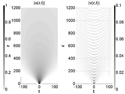
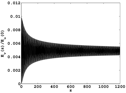
Figure 1: (a) Absolute values $|u(z,t)|$ and $|v(z,t)|$, as functions of the propagation distance, $z$, and temporal coordinate, $t$, obtained from the numerical solution of the linear version of Eqs. (1) and (2) with initial conditions (32), in the case of weak coupling, $\gamma=0.1$, $q=1$. (b) The evolution of the integral energy of the $v$ component, defined as per Eq. (4) and normalized to the initial energy. The evolution of energy of the $u$ component is essentially the same, according to Eq. (5).

Next, we consider the situation close to the $\mathcal{CPT}$-symmetry-breaking threshold (11), namely, with $\gamma=0.9$ for $q=1$. The respective numerical solution, generated by initial conditions (32), is displayed in Fig. 2, which, naturally, demonstrates strong coupling between the two components and more dramatic evolution. In this case too, the asymptotic stage of the evolution for broad pulses is correctly predicted by the above-mentioned analytical approximation.

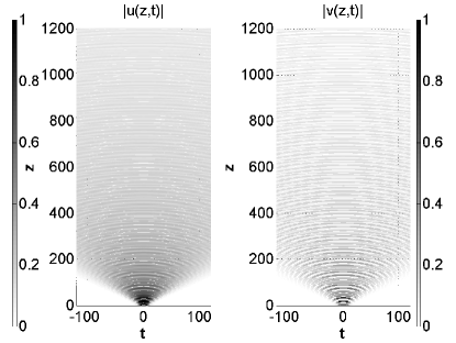
Figure 2: The same as in Fig. 1, but for the strong coupling, $\gamma=0.9$.

To test the symmetry of the system, we have also performed simulations of the evolution starting from initial conditions (33), with swapped components $u$ and $v$. Comparison of the respective results, displayed in Figs. 3(a) and 3(b), with their counterparts shown above in Fig. 2 confirms the symmetry. Furthermore, the detailed comparison of the real and imaginary parts of the two components in both cases (not shown here in detail) exactly corroborates the full $\mathcal{CP}$ symmetry implied by definition (6).

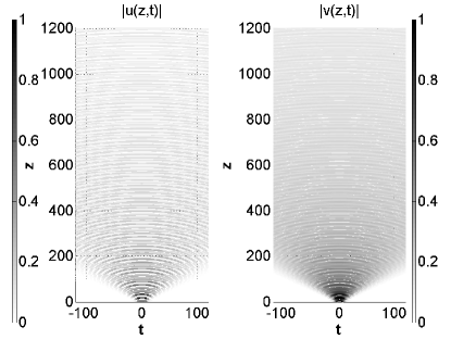
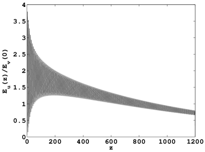
Figure 3: The same as in Fig. 2, but for initial conditions (33), with the difference that panel (b) displays the evolution of the energy in the $u$ component.

For $\gamma>q$, when the the $\mathcal{CP}$ symmetry of the system is broken, according to Eq. (11), direct simulations (not shown here) demonstrate blowup of solutions, as should be expected above the symmetry-breaking point Bender (2003); Ruter et al. (2010b).

The analytical approximation for broad pulses, based on Eqs. (19) and (23), was directly tested by comparing its predictions with the numerically simulated evolution commencing from the initial conditions produced by Eqs. (19) and (23) with $z=0$ and the upper sign in the latter equation. Figure 4 shows that the respective analytical and the numerical results are almost identical. The comparison produces equally good results (not shown here in detail) if the initial conditions are taken, instead, as per Eq. (20) and Eq. (23) with the lower sign, at $z=0$.

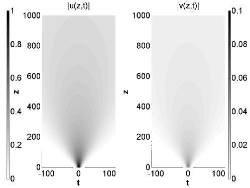
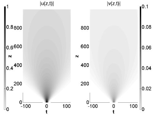
Figure 4: (a) The numerical simulations for absolute values $|u(z,t)|$ and $|v(z,t)|$ in the weak-coupling regime, with $\gamma=0.1$, $q=1$ and the initial conditions taken as per Eqs. (19) and (23) (with the upper sign) at $z=0$. (b) The respective analytical solutions.

On the other hand, for strong coupling, e.g., for $\gamma=0.9$, when $\exp\left(\pm i\sqrt{q^{2}-\gamma^{2}}z\right)$ is no longer a rapidly oscillating carrier in comparison with slowly varying $\tilde{u}$ and $\tilde{v}$, see Eqs. (19) and (20), the analytical approximation is no longer relevant. The comparison with the numerical results corroborates this expectation (not shown here in detail either).

III.2 The nonlinear system

Simulations of the nonlinear system, based on Eqs. (1) and (2), were performed by varying the nonlinearity coefficient, $\sigma$, and (as above) the coupling coefficient, $\gamma$. The initial conditions were taken in the form of Eq. (32), unless stated otherwise.

We start by addressing the weakly coupled system with weak nonlinearity, viz., the one with $0<\sigma\ll 1$ and $0<\gamma\ll q\equiv 1$. For $\gamma=0.1$ and $\sigma=0.1$, Figs. 5(a) and (b) demonstrate that the focusing nonlinearity readily causes self-trapping of a robust oscillating quasi-soliton. Thus, the weak nonlinearity, while breaking the $\mathcal{CP}$ symmetry (see above), creates the self-confined modes.

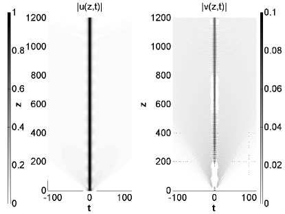
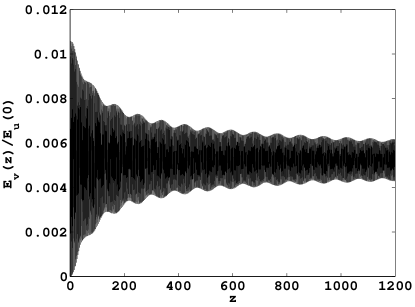
Figure 5: The same as in Fig. 1, but produced by simulations of the full nonlinear system (1), (2) with $q=1$, $\gamma=0.1$, and $\sigma=0.1$. The weak radiation field around the emerging quasi-soliton is virtually invisible, if local powers, $|u(z,t)|^{2}$ and $|v(z,t)|^{2}$, are displayed instead of the amplitudes, $|u(z,t)|$ and $|v(z,t)|$.

Next, we increase the strength of the coupling to $\gamma=0.8$, keeping the nonlinear term small, with $\sigma=0.1$. In this case, Figs. 6(a) and (b) demonstrate strong self-focusing of the modes occurring around $z=10$, followed by the propagation of the confined mode in a sufficiently robust form, although with more conspicuous emission of radiation waves than in the case of $\gamma=0.1$, cf. Fig. 5(a). Thus, in this case too, the system tends to form oscillatory quasi-soliton modes.

The formation of these solitons is readily explained by Eq. (21) for $\tilde{u}$. Indeed, it is easy to check that the width and amplitude of the emerging solitons satisfy conditions (18). The solitons are observed in Figs. 5 and 6 in an oscillatory form, which is different from the stationary solution (24), in accordance with the well-knows fact that perturbed NLS solitons may feature long-lived vibrations, similar to those observed in these figures Anderson (1983); Malomed (2002).

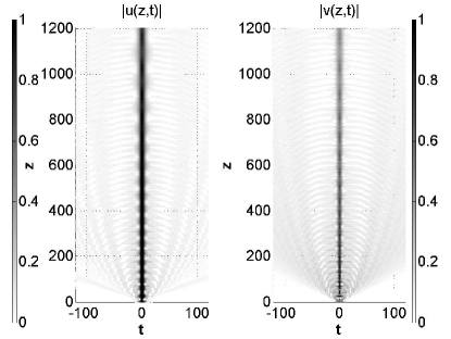
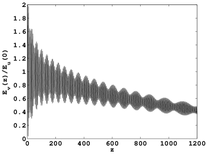
Figure 6: The same as in Fig. 5, but in the case of strong coupling, $\gamma=0.8$.

For $\gamma\geq 0.9$ and the same weak nonlinearity, $\sigma=0.1$, the simulations demonstrate that amplitudes of both modes, $u$ and $v$, diverge after a short propagation distance, which implies that the symmetry breaking takes place in these cases, that are close to the threshold (11) of the symmetry breaking. The small difference of $\gamma=0.9$ from the exact linear threshold, $\gamma=1$, is compensated in this case by the presence of the nonlinearity which, as said above, is also a $\mathcal{CP}$-symmetry-breaking factor.

The swap of initial conditions (32) and (33) in the nonlinear system produces a strong effect. Indeed, in the above simulations, performed for input (32), the pulse was launched in component $u$, where the nonlinearity is self-focusing [see Eq. (1)], while initial conditions (33) imply that the pulse is launched into component $v$ with the self-defocusing cubic term, see Eq. (2). Accordingly, in the latter case, the simulations produce the results displayed in Fig. 7: instead of the quick self-trapping (cf. Fig. 6), the pulse launched in the $v$ component features slow expansion. An additional difference is that the frequency of oscillations observed in the latter case is approximately half of that observed in Fig. 6.

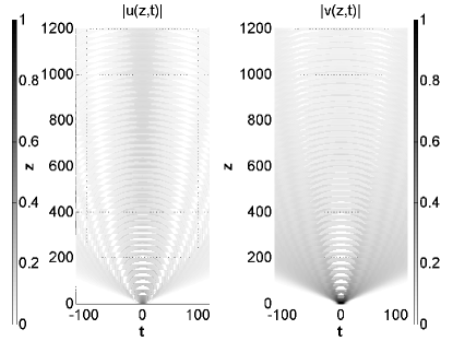
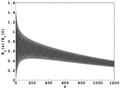
Figure 7: The same as in Fig. 6, but for initial conditions (33).

The increase of $\sigma$ at a fixed coupling constant, $\gamma$, enhances the $\mathcal{CP}$-symmetry-breaking effects, and eventually leads to destruction of the quasi-soliton. In particular, for the weakly coupled system, with $\gamma=0.1$, the destabilization of the quasi-soliton sets in at critical value $\sigma=0.5$, as shown in Fig. 5. In this case, the integral energy slowly grows with $z$, which is followed by blowup at very large values of $z$ (not shown here in detail).

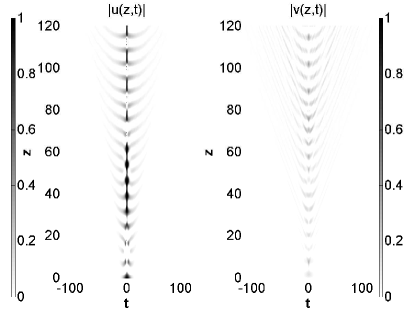
Figure 8: The same as in Fig. 5(a), but at the critical value of the nonlinearity strength, $\sigma=0.5$, at which the gradual destruction of the quasi-soliton commences.

By means of systematical simulations, we have collected the critical values of $\sigma$, at which the quasi-soliton suffers the onset of the destabilization, eventually leading to the blowup, at increasing values of the coupling constant, $\gamma$. The corresponding dependence between $\sigma$ and $\gamma$, shown in Fig. (9), naturally demonstrates that the critical strength of the nonlinearity vanishes when $\gamma$ approaches the threshold of the symmetry breaking in the linear system, $\gamma=1$, see Eq. (11) [recall the normalization is fixed by setting $q=1$ in Eqs. (1) and (2)].

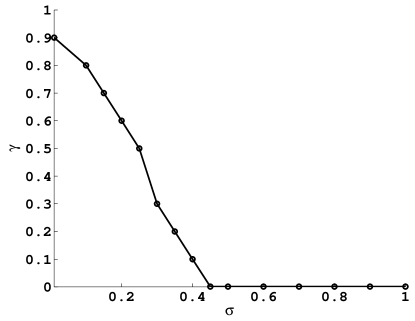
Figure 9: The stability region (beneath the curve) for the oscillatory quasi-solitons created from initial conditions (32), in the plane of $\left(\sigma,\gamma\right)$.

The analytical approximation based on Eqs. (19) and (24) was tested for the broad solitons too. Figure 10 shows that the respective analytical and the numerical results are almost identical, thus validating the analytical approximation for the nonlinear system.

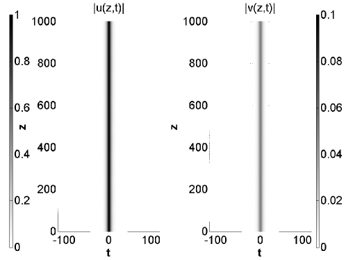
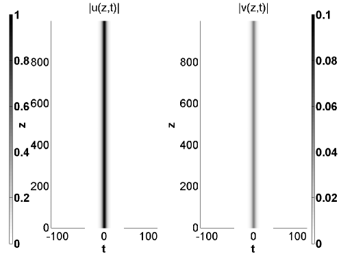
Figure 10: (a) The numerical simulations for absolute values $|u(z,t)|$ and $|v(z,t)|$ in the weakly coupled nonlinear system, with $\gamma=0.1$, $\sigma=0.1$, $q=1$ and initial conditions taken as per Eqs. (19) and (24) with $\kappa=0.05$ at $z=0$. (b) The respective analytical solution.

III.3 Stationary gap solitons in the nonlinear system

The quasi-solitons considered above are built as breathers, featuring permanent oscillations in both components. On the other hand, Eqs. (28-30) predict the existence of stationary gap solitons in the same system. To check this possibility in the numerical form, we solved Eqs. (26-27) by means of the Newton's method Davis (1984). This was done using the approximate analytical solution, given by Eqs. (28) and (30), as the initial guess. The results are produced here for $\sigma=1$ and different values of the coupling constant, $\gamma$.

In the case of weak coupling, $\gamma=0.1$, when it is natural to expect the solutions to be strongly asymmetric, in terms of the two components, the numerical solution at $k=0$, i.e., at the center of the bandgap, is very close to its above-mentioned analytical counterpart, as seen in Fig. 11.

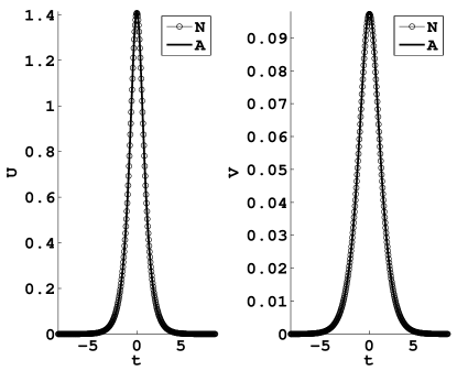
Figure 11: Numerical (“Newton" - N) and analytical solutions (A) for the two components of a strongly asymmetric gap soliton, $U(t)$ and $V(t)$ (note different scales in the panels), obtained from Eqs. (26) and (27) for $q=1$, $\sigma=1$, $\gamma=0.1$, and $k=0$. The respective analytical solution is given by Eq. (28) and (30).

For larger values of $\gamma$, the numerical solution differs from the analytical one, obtained under condition $\gamma\ll q\equiv 1$, although the difference remains relatively small for $\gamma=0.5$, as shown in Fig. 12. The difference becomes essential for $\gamma=0.9$ [in fact, very close to the symmetry-breaking threshold (11)], as can be seen in Fig. 13.

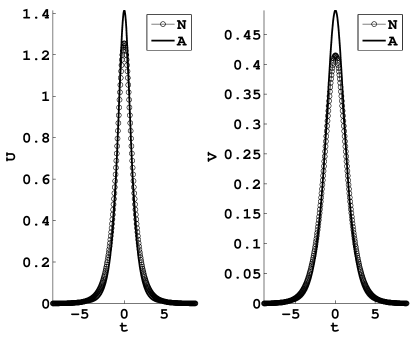
Figure 12: The same as in Fig. 11, but for $\gamma=0.5$.

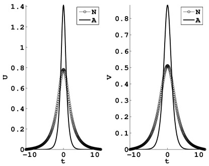
Figure 13: The same as in Fig. 11, but for $\gamma=0.9$.

At $k\neq 0$, the numerically found solutions are still close to the the strongly asymmetric analytical expressions given by Eqs. (28) and (30) for $k=0$, provided that $|k|$ is small enough, see Fig. 14 for $\gamma=0.2$ and $k=0.2$. However, at larger $k$, such as $k=0.8$ with the same $\gamma=0.2$ [note that $k=0.8$ falls into the bandgap (12) in this case], the numerical solution for the $V$ component strongly deviates from the analytical expression given by Eq. (27) for $k=0$, while the $U$ component is still close to the simple analytical form (28), see Fig. 15.

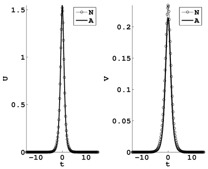
Figure 14: The same as in Fig. 11, but for $\gamma=0.2$, and the numerical solution taken for $k=0.2$ [recall that analytical expression (30) pertains to $k=0$].

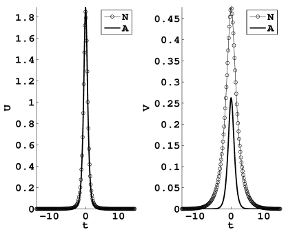
Figure 15: The same as in Fig. 14, but for the numerical solution taken for $k=0.8$.

An analytical solution for strongly asymmetric gap solitons (corresponding to $\gamma\ll 1$) was also obtained above in the form of Eqs. (28) and (31) for $k=-(3/5)q$. For $\gamma=0.1$, this solution is virtually identical to its numerically found counterpart, as shown in Fig. 16.

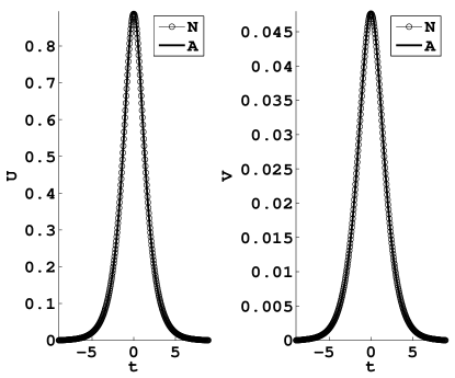
Figure 16: Numerical and analytical solutions for the two components of a strongly asymmetric gap soliton, $U(t)$ and $V(t)$, obtained from Eqs. (26) and (27) for $q=1$, $\sigma=1$, $\gamma=0.1$, and $k=-(3/5)q$. The respective analytical solution is given by Eqs. (28) and (31).

Finally, the stability of the numerically generated gap solitons was tested by using them as initial conditions in direct simulations of Eqs. (1) and (2). The results, not shown here in detail, demonstrate that all the tested examples of gap solitons are stable, both at the center of the gap, $k=0$, and off the center, including values of the coupling constant (such as $\gamma=0.9$) which are close to the symmetry-breaking threshold (11).

IV Conclusions

The objective of this work is to introduce a model of a dual-core waveguide which may implement an optical system featuring the $\mathcal{CP}$ symmetry. Essential ingredients of the model are opposite GVD signs in the two cores, a phase-velocity mismatch between them, and the linear coupling of the gain-loss type, which is possible if the waveguide is embedded into an active medium, or may be provided by the propagation in the $\chi^{(2)}$ medium of the Type-II (three-wave) type, neglecting the depletion of the SH (second-harmonic) pump. Nonlinear cubic terms, which destroy the symmetry, were considered as well (in the case of the $\chi^{(2)}$ medium, they are different from those considered here). It is predicted in an approximate analytical form and demonstrated numerically that the linear system gives rise to expanding Gaussian pulses. Relatively weak nonlinearity produces an essential effect, building broad oscillatory quasi-solitons, which are destroyed in direct simulations if the nonlinearity is too strong. Further, the analysis predicts a general family of stationary gap solitons in the nonlinear system, that have been also found and checked for the stability in the numerical form, the broad solitary pulses being a limit case of the gap solitons near the bottom edge of the bandgap.

The analysis can be continued by considering higher-order modes [it is well known that linear Schrödinger equations (21) give rise to higher modes in the form of Hermite-Gauss wave functions] and interactions between fundamental solitons in the nonlinear version of the system. On the other hand, it was mentioned above that Eq. (21) for $\tilde{v}$ suggests the existence of dark solitons in the present system, which is an interesting issue too. Still another possibility is to consider the different form of the cubic nonlinearity, corresponding to the underlying $\chi^{(2)}$ system. A challenging extension is to consider a two-dimensional version of the model, which may be based on a dual-core planar waveguide embedded into the active medium.

References

- (1)
- Bernabeu (2011) J. Bernabeu, in Journal of Physics: Conference Series (IOP Publishing, 2011), vol. 335, p. 012011.
- Aguilar-Arevalo et al. (2013) A. Aguilar-Arevalo, C. Anderson, A. Bazarko, S. Brice, B. Brown, L. Bugel, J. Cao, L. Coney, J. Conrad, D. Cox, et al., Physics Letters B 718, 1303 (2013).
- Yaffe (2013) L. G. Yaffe, Particles and Symmetries (University of Washington, 2013).
- Bender (2003) C. M. Bender, Annales de l'institut Fourier 53, 997 (2003), eprint 1210.0208.
- Bender et al. (2012) C. Bender, A. Fring, U. Gunther, and H. Jones, Journal of Physics A: Mathematical and Theoretical 45, 440301 (2012).
- Ruschhaupt et al. (2005) A. Ruschhaupt, F. Delgado, and J. G. Muga, Journal of Physics A: Mathematical and General 38, L171 (2005).
- Musslimani et al. (2008) Z. H. Musslimani, K. G. Makris, R. El-Ganainy, and D. N. Christodoulides, Phys. Rev. Lett. 100, 030402 (2008).
- Makris et al. (2008) K. G. Makris, R. El-Ganainy, D. N. Christodoulides, and Z. H. Musslimani, Phys. Rev. Lett. 100, 103904 (2008).
- Longhi (2010) S. Longhi, Phys. Rev. A 81, 022102 (2010).
- Lin et al. (2011) Z. Lin, H. Ramezani, T. Eichelkraut, T. Kottos, H. Cao, and D. N. Christodoulides, Phys. Rev. Lett. 106, 213901 (2011).
- Zhu et al. (2011) X. Zhu, H. Wang, L.-X. Zheng, H. Li, and Y.-J. He, Opt. Lett. 36, 2680 (2011).
- Makris et al. (2011) K. Makris, R. El-Ganainy, D. Christodoulides, and Z. Musslimani, International Journal of Theoretical Physics 50, 1019 (2011).
- Ruter et al. (2010a) C. E. Ruter, K. G. Makris, R. El-Ganainy, D. N. Christodoulides, M. Segev, and D. Kip, 6, 192 (2010a).
- Feng et al. (2011) L. Feng, M. Ayache, J. Huang, Y.-L. Xu, M.-H. Lu, Y.-F. Chen, Y. Fainman, and A. Scherer, Science 333, 729 (2011).
- Regensburger et al. (2012) A. Regensburger, C. Bersch, M.-A. Miri, G. Onishchukov, D. N. Christodoulides, and U. Peschel, Nature 488, 167 (2012).
- Rüter et al. (2009) C. E. Rüter, D. Kip, K. G. Makris, D. N. Christodoulides, O. Peleg, and M. Segev, in Conference on Lasers and Electro-Optics/International Quantum Electronics Conference (Optical Society of America, 2009), p. ITuF2.
- Yu and Fan (2009) Z. Yu and S. Fan (2009), vol. 7220, pp. 72200W–72200W–7.
- Zheng et al. (2010) M. C. Zheng, D. N. Christodoulides, R. Fleischmann, and T. Kottos, Phys. Rev. A 82, 010103 (2010).
- Razzari and Morandotti (2012) L. Razzari and R. Morandotti, Nature (London) 488, 163 (2012).
- Bender et al. (2013) N. Bender, S. Factor, J. D. Bodyfelt, H. Ramezani, D. N. Christodoulides, F. M. Ellis, and T. Kottos, Phys. Rev. Lett. 110, 234101 (2013).
- Abdullaev et al. (2011) F. K. Abdullaev, V. V. Konotop, M. Ogren, and M. P. Sorensen, Optics Letters 36, 4566 (2011), eprint 1111.1310.
- Li et al. (2012) C. Li, H. Liu, and L. Dong, Opt. Express 20, 16823 (2012).
- Suchkov et al. (2011) S. V. Suchkov, B. A. Malomed, S. V. Dmitriev, and Y. S. Kivshar, Phys. Rev. E 84, 046609 (2011).
- Nixon et al. (2012) S. Nixon, L. Ge, and J. Yang, Phys. Rev. A 85, 023822 (2012).
- Zezyulin and Konotop (2012) D. A. Zezyulin and V. V. Konotop, Phys. Rev. Lett. 108, 213906 (2012).
- Leykam et al. (2013) D. Leykam, V. V. Konotop, and A. S. Desyatnikov, Opt. Lett. 38, 371 (2013).
- Driben and Malomed (2011) R. Driben and B. A. Malomed, Opt. Lett. 36, 4323 (2011).
- Alexeeva et al. (2012) N. V. Alexeeva, I. V. Barashenkov, A. A. Sukhorukov, and Y. S. Kivshar, Phys. Rev. A 85, 063837 (2012).
- Driben and Malomed (2011) R. Driben and B. A. Malomed, EPL (Europhysics Letters) 96, 51001 (2011), eprint 1110.2409.
- Moreira et al. (2012) F. C. Moreira, F. K. Abdullaev, V. V. Konotop, and A. V. Yulin, Phys. Rev. A 86, 053815 (2012).
- Moreira et al. (2013) F. C. Moreira, V. V. Konotop, and B. A. Malomed, Phys. Rev. A 87, 013832 (2013).
- Li et al. (2013) K. Li, D. A. Zezyulin, P. G. Kevrekidis, V. V. Konotop, and F. K. Abdullaev, Phys. Rev. A 88, 053820 (2013).
- Skotiniotis et al. (2012) M. Skotiniotis, I. T. Durham, B. Toloui, and B. C. Sanders, ArXiv e-prints (2012), eprint 1201.1594.
- Srednicki (2007) M. Srednicki, Quantum Field Theory (Cambridge University Press, 2007).
- Kursunogammalu et al. (2013) B. Kursunogammalu, S. Mintz, and A. Perlmutter, Confluence of Cosmology, Massive Neutrinos, Elementary Particles, and Gravitation (Springer US, 2013).
- Chaichian et al. (2013) M. Chaichian, K. Fujikawa, and A. Tureanu, Physics Letters B 718, 1500 (2013), eprint 1210.0208.
- Kartashov et al. (2014) Y. V. Kartashov, V. V. Konotop, and D. A. Zezyulin, EPL (Europhysics Letters) 107, 50002 (2014).
- Boardman and Xie (1994) A. D. Boardman and K. Xie, Phys. Rev. A 50, 1851 (1994).
- Kaup and Malomed (1998) D. J. Kaup and B. A. Malomed, J. Opt. Soc. Am. B 15, 2838 (1998).
- Dana et al. (2014) B. Dana, B. A. Malomed, and A. Bahabad, Opt. Lett. 39, 2175 (2014).
- (42) N. M. Litchinitser, I. R. Gabitov, and A. I. Maimistov, Phys. Rev. Lett. 99, 113902 (2007).
- (43) A. I. Maimistov and E.V. Kazantseva, Optika i Spektroskopiya 112, 291 (2012) [English translation: Optics and Spectroscopy 112, 264 (2012)].
- (44) A. A. Dovgiy and A. I. Maimistov, Optika i Spektroskopiya 116, 673 (2014) [English translation: Optics and Spectroscopy 116, 626 (2014)].
- Alexeeva et al. (2014) N. V. Alexeeva, I. V. Barashenkov, K. Rayanov, and S. Flach, Phys. Rev. A 89, 013848 (2014).
- (46) D. A. Zezyulin, V. V. Konotop, and F. Kh. Abdullaev, Opt. Lett. 37, 3930 (2012).
- Agrawal (2001) G. Agrawal, Nonlinear Fiber Optics, Optics and Photonics (Elsevier Science, 2001).
- Tsoy et al. (2014) E. N. Tsoy, I. M. Allayarov, and F. K. Abdullaev, Opt. Lett. 39, 4215 (2014).
- Konotop and Zezyulin (2014) V. V. Konotop and D. A. Zezyulin, Opt. Lett. 39, 5535 (2014).
- Nixon and Yang (2014) S. Nixon and J. Yang, ArXiv e-prints (2014), eprint 1412.6113.
- Ruter et al. (2010b) C. E. Ruter, K. G. Makris, R. El-Ganainy, D. N. Christodoulides, M. Segev, and D. Kip, 6, 192 (2010b).
- (52) G. I. Stegeman, D. J. Hagan, and L. Torner, Opt. Quant. Elect. 28, 1691 (1996),
- (53) and U. Peschel, Progr. Opt. 41, 483 (2000).
- (54) A. V. Buryak, P. Di Trapani, D. V. Skryabin, and S. Trillo, Phys. Rep. 370, 63 (2002).
- (55) H. Suchowski, G. Porat, and A. Arie, Laser Opt. Rev. 8, 333 (1014).
- Kartashov et al. (2014) Y. V. Kartashov, B. A. Malomed, and L. Torner, ArXiv e-prints (2014), eprint 1408.6174.
- de Sterke and Sipe (1994) C. M. de Sterke and J. E. Sipe, Progress in Optics XXXIII 33, 203 (1994).
- Eggleton et al. (1999) B. J. Eggleton, C. M. de Sterke, and R. E. Slusher, J. Opt. Soc. Am. B 16, 587 (1999).
- Blit and Malomed (2012) R. Blit and B. A. Malomed, Phys. Rev. A 86, 043841 (2012).
- Anderson (1983) D. Anderson, Phys. Rev. A 27, 3135 (1983).
- Malomed (2002) B. A. Malomed (Elsevier, 2002), vol. 43 of Progress in Optics, pp. 71 – 193.
- Davis (1984) M. Davis, Numerical methods and modeling for chemical engineers, Wiley series in chemical engineering (Wiley, 1984).