Truncations of a class of pseudo-Hermitian operators

Abstract

We consider the class of non-Hermitian operators represented by infinite tridiagonal matrices, selfadjoint in an indefinite inner product space with one negative square. We approximate them with their finite truncations. Both infinite and truncated matrices have eigenvalues of nonpositive type: either a single one on the real axis or a couple of complex conjugate ones. As a tool to evaluate the reliability of the use of truncations in numerical simulations, we give bounds for the rate of convergence of their eigenvalues of nonpositive type. Numerical examples illustrate our results.

MSC 2010 numbers: 47B36, 47B50

I Introduction

The Hamiltonian $H$ of a physical system represents its energy, which is a real observable. It is therefore required that the expectation values of the quantum operator $H$ be real exep . This can be guaranteed by imposing that $H$ be Hermitian, $H=H^{\dagger}$, as it is known that the spectrum of a Hermitian operator is real and its eigenvectors form a complete orthogonal set dir .

It is on the other hand known that Hermiticity is not a necessary condition for a real spectrum bend : a large number of one-dimensional non-Hermitian potentials, both real and complex, invariant under the simultaneous actions of the parity $P$ (space reflection) and time reflection $T$ operators note have been found to admit energies that are real and discrete.

The matter is not a idle one, as non-Hermitian PT-invariant operators find applications in many areas of theoretical physics: “optical” or “average” potentials in nuclear physics boh , quantum field theories Itz , scattering problems Fesh , localization-delocalization transitions in superconductors Fein , defraction of atoms by standing light waves Berry , as well as the study of solitons on a complex Toda lattice toda .

Unfortunately, PT-invariance is neither necessary nor sufficient to ensure the reality of the spectrum; however, it has been conjectured bend that PT invariant Hamiltonians possess real discrete eigenvalues if the PT symmetry is unbroken i.e. if the energy eigenstates are also eigenstates of the operator PT. When the PT-symmetry is broken and the Hamiltonian is real there instead are energy eigenvalues that are complex conjugate pairs. However, no general condition has been found for the breakdown of the PT-symmetry.

In this contest, it has been pointed out that a necessary, but not sufficient, condition for the spectrum to be real and discrete is the $\eta$-pseudo-Hermiticity, $\eta H\eta^{-1}=H^{\dagger}$, of the Hamiltonian, where $\eta$ is a Hermitian linear automorphism Nevanlinna . The property is also known as selfadjointness in an indefinite inner product space, see bognar ; langerio ; GLR . The eigenvectors of $H$ are in this case $\eta$-orthogonal, i.e. they are orthogonal according to the $\eta$-distorted inner-product $<\psi|\eta\psi>$.

Several PT-symmetric potentials have been found to be P-pseudo-Hermitian Most and classes of non-Hermitian Hamiltonians -both PT-symmetric and non-PT-symmetric- appear to be pseudo-Hermitian under $\eta=e^{-\theta p}$ where $\theta\in\mathbb{R}$ and $p=−i\frac{d}{dx}$ , ($\hbar=1$) is the momentum operator (the transformation generated by $\eta$ is an imaginary shift: $\eta x\eta^{-1}=x+i\theta$, $\eta p\eta^{-1}=p$) Ahmed , or $\eta=e^{-\varphi(x)}$ where $\varphi(x)$ is a $C^{1}$ function of $x$ (the transformation is a complex gauge-like one) Ahmed2 .

It is thus still a case by case procedure to check whether the eigenvalues of an operator are all real. This does not usually cause big practical problems when dealing with a single operator. The situation changes when we have to consider classes of operators. Procedures have been developed for families of operators acting on spaces with finite bases, see e.g. Ref. Weig whose author considers a one parameter family of PT-symmetric matrices $M(\varepsilon)$, with a perturbation parameter $\varepsilon\in\mathbb{R}$ which destroys Hermiticity while it respects PT-invariance.

Here we consider the case when for numerical simulations an operator $H$ acting on a space with an infinite basis needs to be truncated and study the rate of convergence to their asymptotic value of those eigenvalues that for truncated matrices may happen to be non-real. The operator $H=H_{[0,\infty)}$ is given by a non-symmetric Jacobi matrix

$$H_{[0,\infty)}=\begin{pmatrix}a_{0}&-b_{0}&&\\ b_{0}&a_{1}&b_{1}&\\ &b_{1}&a_{2}&b_{2}\\ &&b_{2}&a_{3}&\ddots\\ &&&\ddots&\ddots\\ \end{pmatrix},$$ (I.1)

with bounded, real sequences $(a_{j})_{j=0}^{\infty}$, $(b_{j})_{j=0}^{\infty}$, the sequence $(b_{j})_{j=0}^{\infty}$ being additionally strictly positive. Its finite truncations are of the form

$$H_{[0,n]}=\begin{pmatrix}a_{0}&-b_{0}&&\\ b_{0}&a_{1}&b_{1}&\\ &b_{1}&a_{2}&\ddots\\ &&\ddots&\ddots&b_{n-1}\\ &&&b_{n-1}&a_{n}\\ \end{pmatrix},$$ (I.2)

and

$$\eta={\rm diag\,}(-1,1,1,\dots).$$

Due to the fundamental theorem of Pontryagin pontriagin each the operators $H_{[0,n]}$ has, generically, either a unique single eigenvalue $\lambda_{n}$ on the real axis with the eigenvector $f_{n}$ satisfying $\left<f_{n}|\eta f_{n}\right>\leq 0$ or a single couple of complex conjugate eigenvalues $\lambda_{n}\in\mathbb{C}^{+}$, $\bar{\lambda}_{n}\in\mathbb{C}^{-}$ (to avoid confusion with the conventions used in some of the papers we quote, we note that here and in the following $\left<x|y\right>$ always denotes the usual inner product –either in $\mathbb{C}^{n}$ or in $\ell^{2}$– linear with respect to the second variable). The remaining part of the spectrum of $H_{[0,n]}$ is real. The same is true for the spectrum of the infinite matrix $H_{[0,\infty]}$ with the eigenvalue $\lambda_{\infty}$, see Section II for details. The character of the convergence $\lambda_{n}\to\lambda_{\infty}$ is the main topic of our paper.

Our approach makes use of analytic representations of the function

$$m_{[0,\infty)}(z)=-\left<e_{0}|(H_{[0,\infty)}-z)^{-1}e_{0}\right>,$$ (I.3)

which contains the full information about the spectrum of $H_{[0,\infty)}$ and of its $[n-1/n]$ Padé approximants

$$m_{[0,n]}(z)=-\left<e_{0}|(H_{[0,n]}-z)^{-1}e_{0}\right>.$$ (I.4)

In particular, $\lambda_{n}$ ($\lambda_{\infty}$) is a pole of $m_{[0,n]}(z)$ ($m_{[0,\infty]}$, respectively) and it can be characterized in analytic terms. Due to the locally uniform convergence of $m_{[0,n]}$ to $m_{[0,\infty)}$ DD07 , the sequence $(\lambda_{n})_{n=0}^{\infty}$ converges to $\lambda_{\infty}$ (Corollary II.5). Our main interest is the rate of this convergence. In particular we show its dependence of the placement of the eigenvalue $\lambda_{\infty}$ in $\mathbb{C}^{+}\cup\mathbb{R}$.

Our paper is organized as follows:

• We give various analytic representations of the function (I.3), choosing in particular as our starting point

  $$\frac{-1}{m_{[0,\infty)}(z)}={a_{0}-z+b_{0}^{2}\int_{t_{3}}^{t_{4}}\frac{d\mu(t)}{t-z}},$$

  where $\mu$ is some probability measure, see Theorem II.1.

• In the case $\lambda_{\infty}\notin[t_{3},t_{4}]$ we show that the convergence rate of $\lambda_{n}$ to $\lambda_{\infty}$ is exponential, with the base of the exponent increasing with the distance of $\lambda_{\infty}$ from $[t_{3},t_{4}]$: see Theorem III.3 below.

• However, the $\lambda_{n}$’s tend to arrange themselves in branches spiraling into $\lambda_{\infty}$ and some of these branches can get trapped in the real axis for a number of iterations $n_{0}$ which can be relatively large when $\lambda_{\infty}$ is close to $[t_{3},t_{4}]$. We show examples with different numbers of branches and compute an estimate for $n_{0}$ in Theorem A.1.

• In the case when $\lambda_{\infty}\in[t_{3},t_{4}]$ we build an example to show that the convergence rate is in general worse than exponential.

• In the concluding remarks we review the possible cases from the numerical point of view.

II Holomorphic representations of the $m$-function

We start with reviewing the spectral properties of the matrices $H_{[0,n]}$ and $H_{[0,\infty]}$. The matrix $H_{[0,n]}$ is selfadjoint in the indefinite inner-product space with the fundamental symmetry given by $\eta_{n}=[-1]\oplus I_{n}$ ($\eta_{n}$-pseudo-Hermitian). Consequently one of the following four possibilities applies:

• $H_{[0,n]}$ is similar to a diagonal matrix with real entries, except two complex conjugate entries $\lambda_{n}\in\mathbb{C}^{+}$, $\bar{\lambda}_{n}\in\mathbb{C}^{-}$. The eigenvectors $f_{n},g_{n}$ corresponding to the eigenvalues $\lambda_{n},\bar{\lambda}_{n}$ of $H_{[0,n]}$ satisfy $\left<f_{n}|\eta_{n}f_{n}\right>=\left<g_{n}|\eta_{n}g_{n}\right>=0$, $\left<f_{n}|\eta_{n}g_{n}\right>\neq 0$.

• $H_{[0,n]}$ is similar to a diagonal matrix with real entries and there is precisely one eigenvalue $\lambda_{n}$ with the corresponding eigenvector $f_{n}$ satisfying $\left<f_{n}|\eta_{n}f_{n}\right><0$.

• $H_{[0,n]}$ is similar to a block-diagonal matrix with all the blocks real and one-dimensional, except one block of the form

  $$\begin{pmatrix}\lambda_{n}&1\\ 0&\lambda_{n}\end{pmatrix}\text{ with }\lambda_{n}\in\mathbb{R}.$$

  The eigenvector $f_{n}$ corresponding to the eigenvalue $\lambda_{n}$ of $H_{[0,n]}$ satisfies $\left<f_{n}|\eta_{n}f_{n}\right>=0$.

• $H_{[0,n]}$ is similar to a block-diagonal matrix with all the blocks real and one-dimensional, except one block of the form

  $$\begin{pmatrix}\lambda_{n}&1&0\\ 0&\lambda_{n}&1\\ 0&0&\lambda_{n}\end{pmatrix}\text{ with }\lambda_{n}\in\mathbb{R}.$$

  The eigenvector $f_{n}$ corresponding to the eigenvalue $\lambda_{n}$ of $H_{[0,n]}$ satisfies $\left<f_{n}|\eta_{n}f_{n}\right>=0$.

The cases (iii) and (iv) are non-generic, i.e. the set of all matrices $H_{[0,n]}$ for which one of them applies has measure zero. We refer the reader to GLR for the full canonical form of matrices selfadjoint in indefinite inner-product spaces, which gives also a full description of the eigenvectors. We observe that the matrix $H_{[0,n]}$ may jump back and forth with $n$ among the four types above.

The spectral properties of the infinite matrix $H_{[0,\infty)}$, understood as an operator on $\ell^{2}$, are more tricky: we refer the reader to JL85 ; JLT for a full description and for canonical models. Here we note only that again there are essentially two possibilities:

• $H_{[0,\infty)}$ is similar to an orthogonal sum of a bounded selfadjoint operator in a Hilbert space and a diagonal matrix with two complex conjugate entries $\lambda_{n}\in\mathbb{C}^{+}$, $\bar{\lambda}_{n}\in\mathbb{C}^{-}$. The eigenvectors $f_{n},g_{n}$ corresponding to the eigenvalues $\lambda_{n},\bar{\lambda}_{n}$ of $H_{[0,\infty)}$ satisfy $\left<f_{n}|\eta_{n}f_{n}\right>=\left<g_{n}|\eta_{n}g_{n}\right>=0$, $\left<f_{n}|\eta_{n}g_{n}\right>\neq 0$.

• The spectrum of $H_{[0,\infty)}$ is real and $H_{[0,\infty)}$ has a (unique) real eigenvalue with the corresponding eigenvector $f_{\infty}$ satisfying $\left<f_{\infty}|\eta f_{\infty}\right>\leq 0$.

In the (ii’) case the Jordan chain corresponding to $\lambda_{\infty}$ is again of length not greater than three.

Now we specify the theory developed in De03 ; DD04 ; DD07 to the case we are dealing with in the present work. Besides the matrices $H_{[0,\infty)}$ and $H_{[0,n]}$ defined in (I.1) and (I.2), we shall use the following truncations of the matrix $H_{[0,\infty)}$

$$H_{[1,n]}=\begin{pmatrix}a_{1}&b_{1}&\\ b_{1}&a_{1}&\ddots\\ &\ddots&\ddots&b_{n-1}\\ &&b_{n-1}&a_{n}\\ \end{pmatrix},\qquad n=1,2,\dots.$$ (II.1)

Furthermore, $H_{[1,\infty)}$ will stand for the infinite, symmetric Jacobi matrix with $(a_{j})_{j=1}^{\infty}$ on the main and $(b_{j})_{j=1}^{\infty}$ on the second diagonals. Similarly to (I.3) and (I.4) we define the functions

$$m_{[1,n]}(z)=\left<e_{1}|(H_{[1,n]}-z)^{-1}e_{1}\right>,\quad m_{[1,\infty)}(z)=\left<e_{1}|(H_{[1,\infty)}-z)^{-1}e_{1}\right>.$$ (II.2)

Here $e_{j}$ stands for the $j$–th vector of the canonical basis of $\ell^{2}$. We call the functions appearing in (I.3), (I.4) and (II.2) the $m$–functions of the corresponding Jacobi matrix. We refer the reader to GS for a treatment of $m$–functions of symmetric Jacobi matrices appearing in (II.2). The functions $m_{[1,n]}$ ($n\in\mathbb{Z}_{+}$) and $m_{[1,\infty)}$ are analytic in the open upper half-plane $\mathbb{C}^{+}$. The function $m_{[0,\infty)}$ ($m_{[0,n]}$) is analytic in the upper half-plane, except $\lambda_{\infty}$ ($\lambda_{n}$, respectively).

Moreover, the Schur complement argument provides the following crucial relations DD04 ; GS

$$m_{[0,n]}(z)=\frac{1}{z-a_{0}-b_{0}^{2}\ m_{[1,n]}(z)},\quad z\in{\mathbb{C}}^{+}\setminus\{\lambda_{n}\},\ n\in\mathbb{Z}_{+},$$ (II.3)

$$m_{[0,\infty)}(z)=\frac{1}{z-a_{0}-b_{0}^{2}\ m_{[1,\infty)}(z)},\quad z\in{\mathbb{C}}^{+}\setminus\{\lambda_{\infty}\}.$$ (II.4)

Let us now recall the definition of the class $\mathcal{N}_{1}$. By $\mathcal{N}_{1}$ we define the set of generalized Nevanlinna functions with one negative square, that is the functions of one of the three forms

$$\frac{(z-\alpha)(z-\overline{\alpha})}{(z-\beta)(z-\overline{\beta})}\varphi(z),$$ (II.5)

$$\frac{1}{(z-\beta)(z-\overline{\beta})}\varphi(z),$$ (II.6)

$${(z-\alpha)(z-\overline{\alpha})}\varphi(z),$$ (II.7)

where $\alpha$, $\beta$ are complex numbers and $\varphi$ is a Nevanllina function, i.e. $\varphi$ is holomorphic in ${\mathbb{C}}_{+}$ and maps ${\mathbb{C}}_{+}$ into ${\mathbb{C}}^{+}\cup\mathbb{R}$. We refer the reader to DHS1 ; DLLSh for equivalent definitions. Let us now formulate the theorem which fixes the subclass of $\mathcal{N}_{1}$ functions to be investigated in the present work:

Theorem II.1

Let $m$ be a meromorphic function in the open upper half plane. The following conditions are equivalent.

• There exist $\lambda_{\infty}\in\mathbb{C}^{+}\cup\mathbb{R}$, $d\in\mathbb{R}$ and a nontrivial Borel measure $\sigma$ having all moments finite and supported on an interval $[t_{1},t_{2}]$ such that

  $$m(z)=\frac{1}{(z-\lambda_{\infty})(z-\overline{\lambda}_{\infty})}\left(z+d+\int_{t_{1}}^{t_{2}}\frac{d\sigma(t)}{t-z}\right),$$ (II.8)

• There exist $a_{0}\in\mathbb{R}$, $b_{0}>0$ and a nontrivial Borel probability measure $\mu$ having all moments finite and supported on an interval $[t_{3},t_{4}]$ such that

  $$\frac{-1}{m(z)}={a_{0}-z+b_{0}^{2}\int_{t_{3}}^{t_{4}}\frac{d\mu(t)}{t-z}}$$ (II.9)

• There exist a matrix $H_{[0,\infty)}$ of the form (I.1) with bounded entries $a_{j}\in\mathbb{R}$, $b_{j}>0$, $j\in\mathbb{Z}_{+}$ such that

  $$m(z)=m_{[0,\infty)}(z):=-\left<e_{0}|(H_{[0,\infty)}-z)^{-1}e_{0}\right>.$$ (II.10)

Furthermore, the parameters $\lambda_{\infty}$ and $d$ and the measure $\sigma$ in (i), $a_{0},b_{0}$ and $\mu$ in (ii), and $a_{j},b_{j}$, $j\in\mathbb{Z}_{+}$ in (iii) are uniquely determined; the numbers $a_{0}$ and $b_{0}$ in statements (ii) and (iii) coincide and $\lambda_{\infty}$ from statement (i) is the (unique) eigenvalue of nonpositive type of the operator $H_{[0,\infty)}$ from statement (iii).

• The equivalence (ii)$\Leftrightarrow$(iii) is a consequence of equation (II.4) and the classical theory which sets a correspondence between the functions $m_{[1,\infty)}$ and the Jacobi matrices $H_{[1,\infty)}$, see e.g. Ach61 ; GS .

  (iii)$\Rightarrow$(i) Let $m=m_{[0,\infty)}$. From the construction in JL85 it follows that $m$ belongs to the class $\mathcal{N}_{1}$ and hence it has one of the forms (II.5)–(II.7).

  Furthermore, expanding the resolvent into a geometric series at infinity one sees that $m$ necessarily possesses an asymptotic expansion at infinity

  $$m(z)=-\left<e_{0}|(H_{[0,\infty)}-z)^{-1}e_{0}\right>=\frac{1}{z}-\frac{s_{1}}{z^{2}}-\dots-\frac{s_{2n}}{z^{2n+1}}-\cdots,$$ (II.11)

  with $s_{j}\in\mathbb{R}$ ($j=1,2,\dots$) (see DD04 ; DD07 ). Comparing the forms (II.5)–(II.7) with (II.11), one gets by the Hamburger–Nevanlinna theorem Ach61 that the function $\varphi$ in (II.5)–(II.7) can be represented in the form

  $$\varphi(z)=z+d+\int_{t_{1}}^{t_{2}}\frac{d\sigma(t)}{t-z},$$ (II.12)

  where $d\in{\mathbb{R}}$, and $\sigma$ is a measure with all moments finite. Furthermore, comparing the expansions of (II.5), (II.6) and (II.7) with (II.11) we can see that case (II.6) applies. In consequence,

  $$m(z)=\frac{1}{(z-\lambda_{\infty})(z-\overline{\lambda}_{\infty})}\left(z+d+\int_{t_{1}}^{t_{2}}\frac{d\sigma(t)}{t-z}\right),$$ (II.13)

  Observe that the measure $\sigma$ cannot be a finitely supported (trivial) measure, since $b_{j}>0$ for all $j\in\mathbb{Z}_{+}$ and in consequence neither $m_{[1,\infty)}$ nor $m_{[0,\infty)}$ are rational functions. The uniqueness of the parameters $\lambda_{\infty}$ and $d$ and of the measure $\sigma$ follows from the theory of $\mathcal{N}_{1}$ functions, see e.g. DHS1 . The fact that $\lambda_{\infty}$ is the unique eigenvalue of nonpositive type of $H_{[0,\infty)}$ follows e.g. from Ref. DD07 or JL85 .

  (i)$\Rightarrow$(ii) Using the algorithm proposed in De03 (see also ADL07 ), one can find that $m$ defined by (II.13) can be uniquely represented as

  $$m(z)=\frac{1}{z-a_{0}-b_{0}^{2}\ m_{1}(z)},$$ (II.14)

  where $m_{1}(z)=\int_{t_{3}}^{t_{4}}\frac{d\mu(t)}{t-z},$ is a Nevanlinna function with finite moments. $\Box$

Remark II.2

Already at this point we can say something about the influence of the the measure $\mu$ (spectrum of the matrix $H_{[1,\infty)}$) on the position of $\lambda_{\infty}$.

1) Conditions (i) and (ii) in Ref. JL85 tell us that $\lambda_{\infty}\in[t_{3},t_{4}]$ if and only if

$$\int_{t_{3}}^{t_{4}}|t-\lambda_{\infty}|^{-2}d\mu(t)\leq b_{0}^{-2},\qquad a_{0}-{\lambda_{\infty}}+b_{0}^{2}\int_{t_{3}}^{t_{4}}(t-{\lambda_{\infty}})^{-1}d\mu(t)=0.$$ (II.15)

(In particular, since $b_{0}$ is strictly positive, for the first of these conditions to be true, $|t-\lambda_{\infty}|^{-2}$ needs to be a $\mu$-integrable function; the second condition is just the specialization of eq. (II.9) to the case $z=\lambda_{\infty}$ and we introduce it here to fully characterize $\lambda_{\infty}$ itself). It follows that if the measure $\mu$ is sufficiently dense $\lambda_{\infty}$ cannot be on $[t_{3},t_{4}]$, i.e. $\mu$ “repels” the point $\lambda_{\infty}$. This is the case for Examples III.4 and III.5 below.

2) If instead $\mu$ has gaps, these gaps tend to trap $\lambda_{\infty}$. To see this, let’s assume that the spectrum of $H_{[1,\infty)}$ has a gap $(t_{5},t_{6})\subset[t_{3},t_{4}]$ and that $a_{0}\in(t_{5},t_{6})$. From the definition of $H_{[0,\infty)}$, eq. (I.1), it’s obvious that for $b_{0}=0$ the point $a_{0}$ is an eigenvalue of $H_{[0,\infty)}$ with the corresponding eigenvector $f$ satisfying $\left<f|\eta f\right>\leq 0$, i.e. $a_{0}=\lambda_{\infty}$. We now increase $b_{0}=0$; applying Rouché’s theorem to $-1/m_{[0,\infty)}$ and remembering that if $\lambda_{\infty}\notin\mathbb{R}$ then $\bar{\lambda}_{\infty}$ is also an eigenvalue, we see that $\lambda_{\infty}$ moves along the real axis until it meets another part of the spectrum of $H_{[0,\infty)}$ (that is either an eigenvalue, or a part of the continuous spectrum, see Ref. SWW11 ; SWW14 for a detailed analysis of a similar problem). This means that if $\lambda_{\infty}\in(t_{5},t_{6})$, then for a small change of parameters $a_{0},b_{0}$ the eigenvalue $\lambda_{\infty}$ stays in the gap. We shall see one such case in Example III.6.

As already mentioned, $m_{[0,n]}$ is the $[n/n+1]$ Padé approximant of $m_{[0,\infty)}$ and it is an $\mathcal{N}_{1}$ function for $n\geq 1$. Consequently it can be represented in one of the forms (II.5)–(II.7). As we have just done in Theorem II.1 for $m_{[0,\infty)}$, one can specify this representation:

Proposition II.3

Each function $m_{[0,n]}$ $(n=1,2,\dots)$ admits a representation

$$m_{[0,n]}(z)=\frac{1}{(z-\lambda_{n})(z-\overline{\lambda}_{n})}\left(z+d_{n}+\int\frac{d\mu_{n}(t)}{t-z}\right),$$ (II.16)

with $\lambda_{n}\in\mathbb{C}^{+}$, $d_{n}\in\mathbb{R}$ and $\mu_{n}$ a finitely supported measure. Furthermore, the parameters $\lambda_{n}$ and $d_{n}$ and the measure $\mu_{n}$ are uniquely determined and $\lambda_{n}$ is the unique eigenvalue of nonpositive type of $H_{[0,n]}$.

The details of the proof of uniqueness can be found e.g. in DLLSh ; L ; DHS1 . The uniqueness in both Theorem II.1 and Proposition II.3 guaranties that $\lambda_{n}$ ($n=1,2,\dots$) and $\lambda_{\infty}$ are properly defined. In the literature they are called the generalized poles of nonpositive type of the corresponding $\mathcal{N}_{1}$ function, see L . Using the classical result saying that $m_{[1,n]}$ converges to $m_{[1,\infty]}$, see GS ; Ach61 ; Simon98 , one can prove –via eq. (II.3)– the following convergence result, cf. DD07 :

Proposition II.4

The functions $m_{[0,n]}$ $(n\in\mathbb{Z}_{+})$ converge to $m_{[0,\infty)}$ as $n\to\infty$, locally uniformly on ${\mathbb{C}}_{+}\setminus([t_{1},t_{2}]\cup\left\{\lambda_{\infty}\right\})$.

Further generalization to different types of $\eta$-selfadjoint Jacobi matrices can be found in DD07 . As a consequence we have the following corollary (cf. LaLuMa ):

Corollary II.5

The pole $\lambda_{n}$ of $m_{[0,n]}$ converges to the pole $\lambda_{\infty}$ of $m_{[0,\infty)}$ as $n\to\infty$.

• If $\lambda\in{\mathbb{C}}_{+}$ or is an isolated eigenvalue then this statement is a simple consequence of Proposition II.4 and the Rouché theorem.

  If instead $\lambda_{\infty}$ is real and is not an isolated eigenvalue then from Proposition II.4 and the Rouché theorem we see that all the accumulation points of $\lambda_{n}$ lie in the spectrum of $H_{[0,\infty)}$, which is a compact set. Since both the functions $m_{[0,n]}$ and $m_{[0,\infty)}$ belong to $\mathcal{N}_{1}$ and are of the type (II.6), we have

  $$m_{[0,n]}(z)=\frac{1}{(z-\lambda_{n})(z-\overline{\lambda}_{n})}\varphi_{n}(z),\quad m_{[0,\infty)}(z)=\frac{1}{(z-\lambda_{\infty})(z-\overline{\lambda}_{\infty})}\varphi(z),$$

  where $\varphi_{n}$ and $\varphi$ are Nevanlinna functions and $r_{n}$ and $r$ are rational functions. Suppose now that there is a sub-sequence such that $\lambda_{n_{k}}\to\lambda_{0}\neq\lambda_{\infty}$. As a consequence, $\varphi_{n_{k}}$ should also converge to a Nevanlinna function $\varphi_{0}\neq\varphi$ which contradicts the uniqueness of $\varphi$. $\Box$

III Convergence rates

Now we are in a position to ask the principal question of this paper:

• What is the character of the convergence of $\lambda_{n}\to\lambda_{\infty}$?

We mainly consider the situation when $\lambda_{\infty}$ is simple eigenvalue located outside the support of the measure $\mu$ in (II.9): we show a theoretical bound on the convergence rate and test it on examples.

III.1 Theoretical results

In this section we consider the situation when $\lambda_{\infty}$ is a simple pole of $m$. Note that if $\lambda_{\infty}\in\mathbb{C}^{+}$, then it is necessarily a simple pole, due to Theorem II.1 (i); moreover, there exists $n_{0}\in\mathbb{N}$ such that $\lambda_{n}\in\mathbb{C}^{+}$ for $n>n_{0}$ (see Theorem A.1 below). If instead $\lambda_{\infty}$ is a simple real pole, we show that $\lambda_{n}$ is real for sufficiently large $n$. We begin with a technical result, needed to prove our main theorem.

Proposition III.1

Let $m=m_{[0,\infty)}$ satisfy the (equivalent) conditions (i), (ii), (iii) of Theorem II.1. If $\lambda_{\infty}\in\mathbb{C}\setminus[t_{3},t_{4}]$ is a simple pole of $m$, then

$${\lambda_{\infty}-\lambda_{n}}=-\frac{b_{0}^{2}\left(m_{[1,\infty)}(\lambda_{\infty})-m_{[1,n]}(\lambda_{\infty})\right)}{1-b_{0}^{2}m_{[1,\infty)}^{\prime}(\lambda_{\infty})}+\alpha_{n},$$

where $\alpha_{n}$ is such that

$$\frac{\alpha_{n}}{\sup_{x\in X}|m_{[1,\infty)}(x)-m_{[1,\infty)}(x)|}\to 0,\qquad n\to\infty$$

for any disc $X\subseteq\mathbb{C}^{+}$ containing $\lambda_{\infty}$. If, additionally, $\lambda_{\infty}\in\mathbb{R}$, then $\lambda_{n}\in\mathbb{R}$ for sufficiently large $n$.

• Let $X$ be an open disc, such that $\lambda_{\infty}\in X\subseteq\mathbb{C}^{+}\setminus[t_{3},t_{4}]$. Note that for sufficiently large $n$ the functions

  $$m_{n}(z):=\frac{1}{m_{[0,n]}(z)}=z-a_{0}-b_{0}^{2}m_{[1,n]}(z),$$ (III.1)

  as well as

  $$m_{\infty}(z)=\frac{1}{m_{[0,\infty)}(z)}=z-a_{0}-b_{0}^{2}m_{[1,\infty)}(z)$$ (III.2)

  belong to $\mathcal{C}(X)$, the complex Banach space of continuous functions on $X$ with the supremum norm. Indeed, for sufficiently large $n$ the function $m_{[1,n]}(z)$ has no poles in $X\cap\mathbb{R}$. Also observe that $m_{n}$ converges to $m_{\infty}$ in $\mathcal{C}(X)$, since $m_{[1,n]}(z)$ converges to $m_{[1,\infty)}(z)$ locally uniformly on $\mathbb{C}\setminus[t_{3},t_{4}]$. Consider the mapping

  $$F:\mathcal{C}(X)\times X\ni(m,x)\mapsto m(x)\in\mathbb{C}.$$

  As $\lambda_{\infty}\in\mathbb{C}^{+}$ is a simple pole of $m_{[0,\infty)}$, one has

  $$m_{\infty}^{\prime}(\lambda_{\infty})=(-1/m_{[0,\infty)})^{\prime}(\lambda_{\infty})\neq 0.$$

  Therefore,

  $$\frac{\partial F}{\partial x}(m_{\infty},\lambda_{\infty})=m^{\prime}_{\infty}(\lambda)\neq 0,$$

  and we can apply the implicit function theorem in Banach spaces to the mapping $F$ (see e.g. krantz ). As a result we obtain in a neighborhood $U\times Y$ of $(m_{\infty},\lambda_{\infty})$ a differentiable function $\xi:U\to Y$ such that

  $$\left\{(m,x)\in U\times Y:m(x)=0\right\}=\left\{(m,\xi(m)):m\in U\right\}=0.$$

  We may take $Y$ so small that $Y\subseteq\mathbb{C}\setminus[t_{3},t_{4}]$ and that $m_{\infty}$ has no other zeros in $Y$ except $\lambda_{\infty}$. Note that for sufficiently large $n$ one has $m_{n}\in U$. Hence, on one hand we have that for sufficiently large $n$

  $$m_{n}(\xi(m_{n}))=F(m_{n},\xi(m_{n}))=0,\quad m_{n}(x)\neq 0,\ x\in U\setminus\left\{\xi(m_{n})\right\}.$$

  On the other hand, $\lambda_{n}$ converges to $\lambda_{\infty}$ and $m_{n}(\lambda_{n})=0$. Consequently, $\lambda_{n}=\xi(m_{n})$ for $n$ large enough.

  Now note that

  $$\frac{\partial x}{\partial m}(m_{\infty})m=-\frac{\frac{\partial F}{\partial m}(m_{\infty},x(m_{\infty}))m}{\frac{\partial F}{\partial x}(m_{\infty},x(m_{\infty}))}=-\frac{m(\lambda_{\infty})}{m_{\infty}^{\prime}(\lambda_{\infty})}.$$

  Furthermore,

  $${\lambda_{\infty}-\lambda_{n}} = \frac{\partial x}{\partial m}(m_{\infty}){(m_{\infty}-m_{n})}+\alpha(m_{\infty}-m_{n})$$

  $$= -\frac{m_{\infty}(\lambda_{\infty})-m_{n}(\lambda_{\infty})}{m_{\infty}^{\prime}(\lambda_{\infty})}+\alpha(m_{\infty}-m_{n}),$$

  where $\alpha(h_{n})/\left\|h_{n}\right\|_{\mathcal{C}(X)}\to 0$ with $\left\|h_{n}\right\|_{\mathcal{C}(X)}\to 0$. Set $h_{n}=m_{n}-m_{\infty}$ and

  $$\alpha_{n}=\alpha(m_{\infty}-m_{n})=\lambda_{\infty}-\lambda_{n}+\frac{m_{\infty}(\lambda_{\infty})-m_{n}(\lambda_{\infty})}{m_{\infty}^{\prime}(\lambda_{\infty})}$$

  and note that the right-hand side of the above does not depend on the initial choice of the disc $X$. This finishes the proof of the first statement.

  Now let $\lambda_{\infty}\in\mathbb{R}\setminus[{t_{3}},{t_{4}}]$. By the locally uniform convergence of $m_{n}$ to $m_{\infty}$ and by the Rouché theorem there is a small disc $Z$ with the center in $\lambda_{\infty}$, such that each function $m_{n}(z)$ has precisely one zero $z_{n}$ in $Z$. As $\lambda_{n}$ converges to $\lambda_{\infty}$ we must have $\lambda_{n}=z_{n}$ for large $n$. Therefore, $\lambda_{n}\in\mathbb{R}$, otherwise $\bar{\lambda}_{n}\in Z$ is another zero of $m_{n}$ in $Z$, which is a contradiction. $\Box$

Remark III.2

We are able now to prove the main result of our paper, Theorem III.3. First, though, we would like to stress that there are two equivalent ways of seeing it according to the objects we consider:

A first interpretation takes as its main object the tridiagonal matrix, presented here in a block form

$$H_{[0,\infty)}=\left(\begin{array}[]{c|ccc}a_{0}&-b_{0}&0&\cdots\\ \hline\cr b_{0}&&&\\ 0&&H_{[1,\infty)}&\\ \vdots&&&\\ \end{array}\right);$$

$\lambda_{\infty}$ is then the (unique) eigenvalue of nonpositive type of $H_{[0,\infty)}$, $\lambda_{n}$ is the unique eigenvalue of nonpositive type of the finite truncation $H_{[0,n]}$ of $H_{[0,\infty)}$, and the spectrum of $H_{[1,\infty)}$ is contained, by assumption, in $[t_{3},t_{4}]$.

A second interpretation considers instead a meromorphic function $m(z)$ having the representations (II.8) and (II.9) and its $[n-1/n]$ Padé approximants $m_{[0,n]}$. The point $\lambda_{\infty}$ ($\lambda_{n}$) is then the unique pole of nonpositive type of $m(z)$ ($m_{[0,n]}$, respectively).

In both settings Theorem III.3 gives the convergence rate of $\lambda_{n}$ to $\lambda_{\infty}$, in terms of the “distance” of $\lambda_{\infty}$ from the interval $[t_{3},t_{4}]$: the rate of convergence is at least exponential $\mathcal{O}(q^{-2n})$, where the number $q$ is such that $\lambda_{\infty}$ lies on the ellipse with foci at $t_{3},t_{4}$ and sum of its semi-axes equal to $({t_{4}}-{t_{3}})q/2$. Consequently, as confirmed by our numerical tests below, the convergence rate gets worse the larger is the eccentricity of said ellipse, i.e.: the convergence slows down when $\lambda_{\infty}$ is “close” to the interval $[t_{3},t_{4}]$.

Theorem III.3

Let $\lambda_{\infty}$, $\lambda_{n}$, $t_{3}$, $t_{4}$ be as in Theorem II.1 and Remark III.2 above. If $\lambda_{\infty}\in\mathbb{C}\setminus[t_{3},t_{4}]$ is a simple eigenvalue, then

$$\limsup_{n\to\infty}|{\lambda_{\infty}-\lambda_{n}}|^{1/n}\leq\frac{1}{q^{2}},$$

where $q=g+\sqrt{g^{2}-1}$, and

$$g=\frac{|\lambda_{\infty}-t_{4}|+|\lambda_{\infty}-t_{3}|}{t_{4}-t_{3}}>1$$ (III.3)

is the reciprocal of the eccentricity of the ellipse through $\lambda_{\infty}$ with foci at $t_{3},t_{4}$. If, additionally, $\lambda_{\infty}\in\mathbb{R}$, then $\lambda_{n}\in\mathbb{R}$ for sufficiently large $n$.

• For $R>1$ let $L_{R}$ denote the closed set bounded by the ellipse with foci at ${t_{3}},{t_{4}}$ and the sum of its semi-axes equal to $({t_{4}}-{t_{3}})R/2$. Due to Theorem (2.6.2) in Ref. niso , one has

  $$\limsup_{n\to\infty}\sup_{z\in\mathbb{C}\setminus L_{R}}|m_{[1,n]}(z)-m_{[1,\infty)}(z)|^{1/n}\leq\frac{1}{R^{2}}.$$ (III.4)

  Note that

  $$\lambda_{\infty}\notin L_{R}\iff R<g+\sqrt{g^{2}-1}.$$ (III.5)

  Take any $R\in(1,g+\sqrt{g^{2}-1})$ and a small disc $X$, such that $\lambda_{\infty}\in X\subseteq\mathbb{C}\setminus L_{R}$. From Proposition III.1 we obtain that

  $$|{\lambda_{\infty}-\lambda_{n}}| \leq C_{1}|m_{[1,n]}(\lambda_{\infty})-m_{[1,\infty)}(\lambda_{\infty})|+\alpha_{n}$$

  $$\leq C_{2}\sup_{z\in X}|m_{[1,n]}(z)-m_{[1,\infty)}(z)|,$$

  where $C_{1},C_{2}$ are constants, dependent on $H_{[0,\infty)}$ and $X$ only. As a consequence,

  $$\limsup_{n\to\infty}|{\lambda_{\infty}-\lambda_{n}}|^{1/n}\leq\frac{1}{R^{2}}.$$

  Letting $R\to g+\sqrt{g^{2}-1}$ finishes the proof. $\Box$

Note that Theorem III.3 cannot be easily generalized to the case when $\lambda_{\infty}\in[t_{3},t_{4}]\setminus{\rm supp\,}\mu$. For example, if the support of the measure $\mu$ consists of two disjoint intervals $[t_{3},t_{5}]\cup[t_{6},t_{4}]$ the estimate (III.4), which was the key point in proving Theorem III.3, still holds only outside the ellipse with foci at $t_{3},t_{4}$, the reason being that the union of the poles of the Padé approximants of $\int_{t_{3}}^{t_{4}}(t-z)^{-1}\mu(dt)$ may be dense in $[t_{5},t_{6}]$, see for instance Ref. Suetin02 .

III.2 Examples

In our examples we want to be able to choose the position of $\lambda_{\infty}$; it is therefore convenient to consider cases where it is possible to calculate it without resorting at first to truncated matrices. One way to is look for matrices $H_{[1,\infty)}$ such that the the corresponding functions $m_{[1,\infty)}$ have a closed, analytic form. This will allow us to use (numerical) root finding methods to calculate $\lambda_{\infty}$ solving the equation

$$z-a_{0}-b_{0}^{2}\ m_{[1,\infty)}(z)=0.$$ (III.6)

Remembering that

$$m_{[1,\infty)}=\int_{t_{3}}^{t_{4}}\frac{d\mu(t)}{t-z},$$ (III.7)

this reduces to finding a suitable measure $\mu(t)$ with finite support.

The choice

$$d\mu=d\sigma_{\alpha,\beta}(t)=\chi_{[-1,1]}(t)\cdot\frac{(1-t)^{\alpha}(1+t)^{\beta}dt}{\int_{-1}^{1}(1-s)^{\alpha}(1+s)^{\beta}ds},$$ (III.8)

where $\chi_{[-1,1]}(t)$ is the characteristic function of the interval $[-1,1]$, gives us the matrix $H_{[1,\infty)}$ corresponding to Jacobi polynomials with parameters $\alpha,\beta$. To construct $H_{[1,\infty)}$ we consider the Jacobi orthogonal polynomials, which form an orthogonal basis in $L^{2}(\sigma_{\alpha,\beta})$ and the multiplication operator $p\mapsto xp$ in $L^{2}(\sigma_{\alpha,\beta})$. The three term recurrence relation (4.5.1) and the normalization factors (4.3.3) in Ref. Szego provide the tridiagonal representation $H_{[1,\infty)}$ of the multiplication operator. The spectral theorem for selfadjoint operators guarantees that (III.7) with (III.8) is satisfied.

The choice

$$d\mu=\chi_{[-2,2]}(t)\cdot\frac{\sqrt{4-t^{2}}dt}{2\pi}$$ (III.9)

instead gives the matrix $H_{[1,\infty)}$ with $a_{j}=0$, $b_{j}=1$, $j=1,2,\dots$ corresponding to the orthogonal polynomials associated with the Wigner semicircle measure.

To calculate $\lambda_{n}$ we use Matlab matlab : first, we calculate all eigenvalues and eigenvectors of $H_{[0,n]}$; we then find $\lambda_{n}$ as the only eigenvalue of nonpositive type of $H_{[0,n]}$, i.e. the only eigenvalue which is either in the upper half-plane or is real with the corresponding eigenvector ${\bf x}$ satisfying

$$-|x_{0}|^{2}+\sum_{j=1}^{n}|x_{j}|^{2}\leq 0.$$

A summary of the relevant results for all our examples can be found in Table 1. Only graphs useful to our discussion are shown here; for the remaining cases quoted, pictures can be found in the supplementary files S : the file names there refer to those given in Table 1.

Example III.4

As our first example we take $\alpha=\beta=0$ in eq. (III.8) so that

$$m_{[1,\infty)}=\frac{1}{2}\int_{-1}^{1}\frac{dt}{t-z}=\frac{1}{2}(\log(1-z)-\log(-1-z)),$$ (III.10)

where the branch of the logarithm is chosen in such way that the above function is a Nevanlinna function. In this case $H_{[1,\infty)}$ corresponds, in the way described in the remarks above, to the Legendre polynomials. We now vary the only remaining free parameters $a_{0}$ and $b_{0}$ of $H_{[0,\infty)}$. Note in any case, due to Remark II.2, we have $\lambda_{\infty}\notin[t_{3},t_{4}]=[-1,1]$.

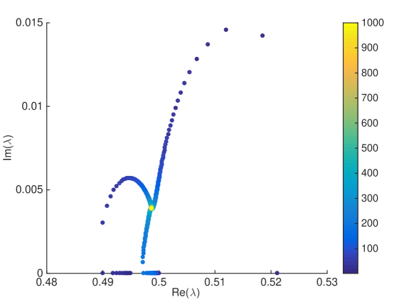
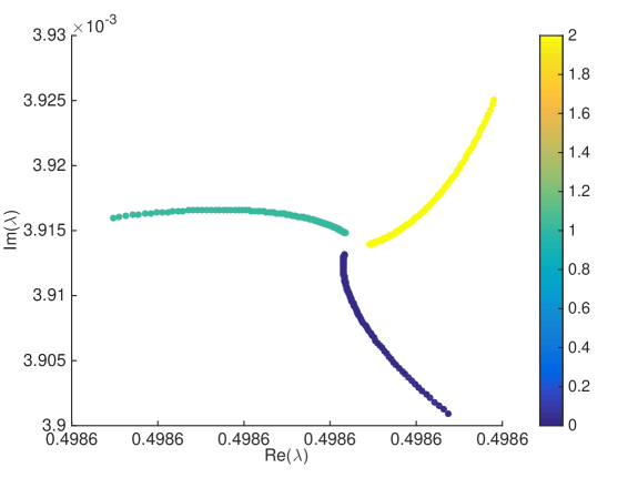
Figure 1: The only eigenvalue $\lambda_{n}$ of nonpositive type of the matrix $H_{[0,n]}$ given in eq. (I.2) with $a_{0}=0.5$, $b_{0}=0.05$ and $H_{[1,n]}$ being the Jacobi matrix corresponding to the Legendre polynomials. The points, each corresponding to a different $n$, are plotted on the complex plane color coded according to $n$ in the upper picture, and according to $n\mod 3$ ($0$–blue, $1$–cyan, $2$–yellow) in the lower picture, where we show a zoomed detail around $\lambda_{\infty}$. The three branches of $\lambda_{n}$ mentioned in the text are clearly visible. See Example III.4.

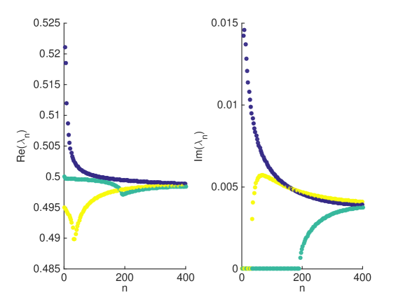
Figure 2: Real and imaginary part of the eigenvalue $\lambda_{n}$ from Figure 1 Vs. $n$. The points color coded according to $n\mod 3$. The cusps in the real parts of the yellow and cyan branches correspond to the change of direction when a branch leaves the real line, see Figure 1. See Example III.4.

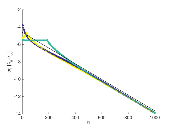
Figure 3: Same parameters as in Figure 1. The black line represents the theoretical bound given in Theorem III.3, shifted down so as to be superimposed on the numerical data. The logarithmic scale on the vertical axis makes evident the exponential convergence of $\lambda_{n}$ to $\lambda_{\infty}$. See Example III.4.

Let us start with $a_{0}=0.5$, $b_{0}=0.05$. It is immediately evident from Figure 1 that the points $\lambda_{n}$ arrange themselves on three branches which spiral into $\lambda_{\infty}$. The point $\lambda_{n}$ jumps in a regular fashion from one branch to another: all $\lambda_{n}$’s with $n\mod 3=\operatorname{const}$ fall on the same branch. The two branches starting on the real axis leave it at $n=45$ and $n=190$ respectively, as can be seen from the plot of the imaginary part of $\lambda_{n}$ in Figure 2; the plots of the corresponding real parts have each a cusp at the same time, due to the inversion of the direction of motion of $\lambda_{n}$. The plot in Figure 3 shows exponential convergence of $\lambda_{n}$ to $\lambda_{\infty}$ setting in soon after all three branches leave the real line. The black reference line with slope $-2\log(q)$ represents the bound from Theorem III.3, the intercept is chosen so that the line is superimposed on the numerical data. In this example (as well as in subsequent examples with measures having no gaps) we see that the estimate of the convergence rate in Theorem III.3 is sharp and consequently can not be improved in general. On the other hand, the estimate is not always sharp, cf. Example III.6.

We have already mentioned that the points $\lambda_{n}$ arrange themselves regularly on branches. This behavior is common to most of our examples, except the cases when $\lambda_{\infty}$ is on the real axis, where because of Proposition III.1 there is one branch only. Since the branches appear to approach $\lambda_{\infty}$ isotropically, as can be e.g. seen in the zoomed picture of Figure 1, this suggests a convenient way of calculating the numerical value of $\lambda_{\infty}$ as the mean

$$\lambda_{\infty}^{(N)}=k^{-1}\sum_{n=N-k+1}^{N}\lambda_{n},$$ (III.11)

where $k$ denotes the number of branches and $N$ the last $n$ for which $\lambda_{n}$ is calculated.

The value of $\lambda_{\infty}$ obtained taking the average of the three last points (one for each branch) equals $0.4999+0.0039\mathrm{i}$, which agrees well with the value $0.498631+0.00391397\mathrm{i}$ obtained solving with Mathematica mathematica eq. (III.6).

We conclude noting that –here and in all our other examples– the real axis forms a barrier for $\lambda_{n}$: it never crosses it and branches which touch it get stuck in it; this is clearly visible in the movie Legendre_spirals_a_0.5.avi that can be found among the supplementary files to this paper S . This behavior is related to the symmetry of the spectrum with respect to the real axis.

If we now keep $a_{0}=0.5$ constant and vary $b_{0}$ to assume the values $b_{0}=0.5,0.1$, and $0.01$, in all cases the $\lambda_{n}$’s arrange themselves over three spiraling branches and the value $\lambda_{\infty}$ obtained from the average of the last three values of $\lambda_{n}$ agrees with the one calculated solving eq. (III.6) with Mathematica to the last digit shown in Table 1. In all cases convergence is exponential and the slope of logarithmic plots similar to that in Figure 3 are in agreement with the value $-2\log(q)$ from Theorem III.3 (see Table 1). There are some case to case differences, but they do not affect the picture given above: for $b_{0}=0.5$ the three branches are not clearly visible, due to the very fast convergence of $\lambda_{n}$; for $b_{0}=0.1$ only one branch spends some time on the real axis, up to $n=46$; and for $b=0.01$ even after 1000 iterations one of the three branches has not yet left the real axis (for figures see the supplementary material S1 ).

Our last example with measure eq. (III.10) is a case when $\lambda_{\infty}\in\mathbb{R}\setminus[t_{3},t_{4}]$: if we take $a_{0}=1.001$ and $b_{0}=0.001$ we get $\lambda_{\infty}\simeq 1.001$ (Mathematica has problems solving eq. (III.6) in this case). The values of $\lambda_{n}$ are all real; we therefore have a single branch. Convergence is again exponential (for figures see the supplementary material S2 ). It is instructive to compare this case to the case $a_{0}=0.5$, $b=0.05$: the distance of $\lambda_{\infty}$ from the interval $[-1,1]$ is of the same order, but the convergence is much faster in the present case. This is due to the different eccentricities of the ellipses from Theorem III.3: in the present case the eccentricity is smaller, and therefore $q$ is larger and in consequence the convergence rate is better.

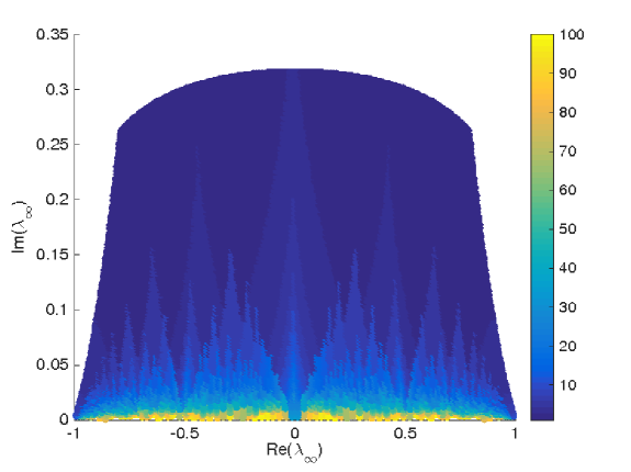
Figure 4: The value $n_{0}$ where the last $\lambda_{n}$ branch leaves the real axis as a function of $\lambda_{\infty}$. $H_{[1,n]}$ is the Jacobi matrix corresponding to the Legendre polynomials and $a_{0}$ and $b_{0}$ vary to get the different values of $\lambda_{\infty}$. See Example III.4.

Finally, in Figure 4 we summarize the convergence behavior when submatrix $H_{[1,\infty)}$ corresponds to measure eq. (III.10): we vary the parameters $a_{0}\in(-1,1)$ and $b_{0}\in(0.05,0.5)$ and for each pair $(a_{0},b_{0})$ we compute the value $n_{0}$ where the last $\lambda_{n}$ branch leaves the real axis. Each pair $(a_{0},b_{0})$ determines a single point $\lambda_{\infty}$ in the upper half-plane, which we plot color coded according to $n_{0}$. The figure appears to have a fractal character for which we do not yet have an explanation but which we suspect to be related to the way the number of $\lambda_{n}$ branches varies with varying $a_{0}$. This can be seen in the movie Legendre_spirals_b_0.01.avi S where we keep $b_{0}=0.01$ and vary $a_{0}$. We instead observe no change in the number of branches when varying $b_{0}$ at constant $a_{0}$ (see e.g. the movie Legendre_spirals_a_0.5.avi S ).

As we have already mentioned, branches are a common occurrence, not limited to the example just given. We give here a couple more examples.

Example III.5

We now take $H_{[1,\infty)}$ corresponding to the orthogonal polynomials associated with the Wigner semicircle measure, i.e. the measure given by eq. (III.9) and we choose $a_{0}=0.5$, $b_{0}=0.1$ as the remaining parameters for $H_{[0,\infty)}$. Note due to Remark II.2 we again have $\lambda_{\infty}\notin[t_{3},t_{4}]=[-2,2]$.

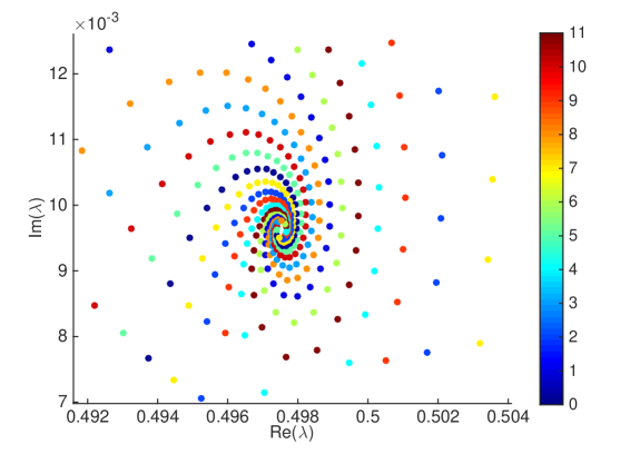
Figure 5: The eigenvalues $\lambda_{n}$ for $H_{[1,n]}$ associated with the Wigner measure and parameters $a_{0}=0.5$, $b_{0}=0.1$, plotted in the complex plane, color coded according to $n\mod 12$ where twelve is the number of $\lambda_{n}$ branches. See Example III.5.

In Figure 5 it is possible to see that the $\lambda_{n}$’s form twelve branches. Knowing this, we can use the recipe given above to calculate $\lambda_{\infty}$ as the mean eq. (III.11) of the last twelve values of $\lambda_{n}$; the result agrees to the last digit shown in Table 1 with the value obtained solving eq. (III.6) with Mathematica.

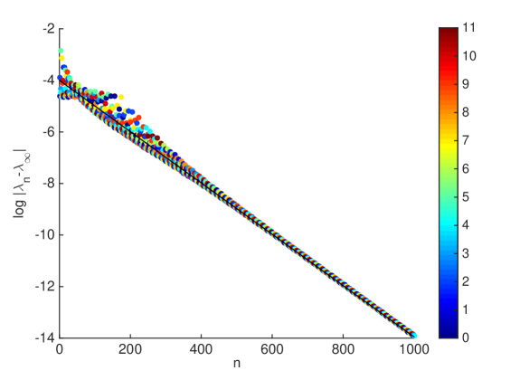
Figure 6: Same parameters and color code as in Figure 5. The black line represents the theoretical bound given in Theorem III.3, shifted down so as to be superimposed on the numerical data. The logarithmic scale on the vertical axis makes evident the exponential convergence of $\lambda_{n}$ to $\lambda_{\infty}$. See Example III.5.

Figure 6 shows exponential convergence of $\lambda_{n}$ to $\lambda_{\infty}$ with the rate predicted by Theorem III.3; other plots concerning this example can be found as supplementary files S3 .

The video Wigner_spirals_b_0.01.avi in S shows the evolution of the $\lambda_{n}$ branches under the change of the parameter $a_{0}$. As in Example III.4, it is evident that here too the number of branches changes with $a_{0}$. Looking at the first few frames of the movie it is also evident that there are branches that start off the real axis, hit it and –instead of continuing into $\mathbb{C}^{-}$– get trapped in it moving horizontally for a number of $n$, and then leave it when the spiral reenters $\mathbb{C}^{+}$.

Example III.6

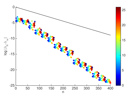
Figure 7: Exponential convergence of $\lambda_{n}$ to $\lambda_{\infty}$. Here $H_{[1,\infty)}$ is associated with a measure on a Cantor-like set and $a_{0}=0.5$, $b_{0}=0.1$. The black line represents the theoretical bound given in Theorem III.3. Color coding according to $n\mod 27$ evidences a repeated pattern of 27 points. The observed convergence is again exponential but much faster than the bound given by Theorem III.3: the observed $q$ is approximately $1.1147$, much larger than the theoretical one $1.0044$. See Example III.6.

Here we present an example of a different nature. The matrix $H_{[1,\infty)}$ is constructed in such way, that its spectrum is a totally disconnected, Cantor-like set, see cantor for details; the other parameters are $a_{0}=0.5$ and $b_{0}=0.1$. In this particular case we could count $27$ branches of $\lambda_{n}$; such a high number is hardly visible when plotting $\lambda_{n}$ in the complex plane but can be seen in the plot of $\log|\lambda_{n}-\lambda_{\infty}|$ in Figure 7: the $\lambda_{n}$’s form regular clusters of $27$ points.

What is particularly noteworthy is that –contrary to the previous examples– the convergence rate is faster than the one predicted by Theorem III.3, as can be seen comparing the theoretical bound (black line) with the numerical points in Figure 7. This is probably due to the fact that the spectrum of $H_{[1,\infty)}$ contains gaps. Other pictures corresponding to this example (called Cantor_a_0.5_b_0.1_xxx.eps), as well as the video Cantor_spirals_b_0.2.avi showing the evolution of branches under the change of the parameter $a_{0}$, can be found in the supplementary files S : again the number of branches changes with $a_{0}$; moreover intervals in $a_{0}$ where both $\lambda_{\infty}$ and all the $\lambda_{n}$ become real are evident and correspond to the gaps in $H_{[1,\infty)}$, see Remark II.2.

Although Theorem III.3 proves the exponential rate of convergence of $\lambda_{n}$ to $\lambda_{\infty}$, it does not say when this convergence starts manifesting itself: at least in theory we could have $|{\lambda_{\infty}-\lambda_{n}}|>q^{-2n}$ for some $n$. Our numerical tests indicate that the convergence is somehow “better” than the above bound, as the asymptotic behavior is $K\cdot q^{-2n}$ with $K<1$. Even the curious initial behavior connected with the real axis we observed in several cases above, does not bring $|{\lambda_{\infty}-\lambda_{n}}|$ to exceed $q^{-2n}$. On the other hand it would be convenient to have an estimate of $n_{0}$ such that for $n>n_{0}$ the point $\lambda_{n}$ is sure to be outside the support $[t_{3},t_{4}]$ of the measure $\mu$: if one or more of the $\lambda_{n}$’s branches is still on $[t_{3},t_{4}]$, our justification for estimating $\lambda_{\infty}$ by the mean eq. (III.11) is compromised. We give an upper bound for $n_{0}$ in Appendix A.

III.3 $\lambda_{\infty}\in\mathbb{R}$ is embedded in the spectrum of the representing measure

We shall limit our investigation of the case when $\lambda_{\infty}\in[t_{3},t_{4}]$ to an example where $\lambda_{\infty}=t_{3}$, to show that convergence in this case is in general worse than exponential. To build our example, we start by recalling Remark II.2. The only example known to us of classical orthogonal polynomials satisfying condition (II.15) with $\lambda_{\infty}\in[t_{3},t_{4}]$ are the Jacobi polynomials with parameters $\alpha\geq 2$ or $\beta\geq 2$ and with $\lambda_{\infty}=t_{3}$ or $\lambda_{\infty}=t_{4}$, respectively.

Example III.7

We take $H_{[1,\infty)}$ such that

$$m_{[1,\infty)}=\int_{-1}^{1}\frac{\frac{3}{4}(1+t)^{2}(1-t)dt}{t-z},$$

i.e. we take $\alpha=2,\beta=1$ in eq. (III.8). We then choose $a_{0}=-5/3$, $b_{0}=\sqrt{2/3}$, so that $\lambda_{\infty}=-1$. This can be seen e.g. by analyzing the matrix $H_{[0,\infty)}$ itself: it results from JL85 conditions (i) and (ii) that $-1$ is an algebraically simple eigenvalue of $H_{[0,\infty)}$ with the corresponding eigenvector $x$ satisfying $-|x_{0}|^{2}+\sum_{j=1}^{\infty}|x_{j}|^{2}=0,$ i.e. $\lambda_{\infty}=-1$ is the unique eigenvalue of nonpositive type of $H_{[0,\infty)}$.

Furthermore, due to Theorem 2.2 ($p_{1s}$) of JL85 , $-1$ is a singular critical, algebraically simple eigenvalue (see JL85 for a classification of eigenvalues of nonpositive type).

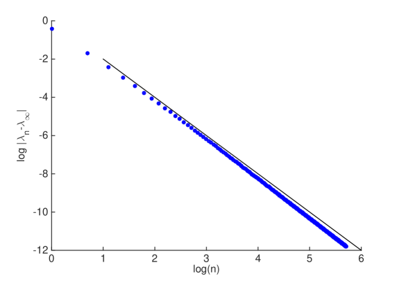
Figure 8: Log-log plot showing $\mathcal{O}(n^{-2})$ convergence of $\lambda_{n}$ to $\lambda_{\infty}=-1$ in a case when $\lambda_{\infty}$ is embedded in the spectrum of $H_{[1,\infty)}$. See Example III.7.

The log-log plot of $|\lambda_{n}-\lambda|$ Vs. $n$ in Figure 8 shows clearly that convergence in this case is only polynomial: $|\lambda_{n}-\lambda|\simeq n^{-2}$, as can be seen comparing the numerical data with the black reference line whose slope is $-2$. The plot of the real and imaginary part of $\lambda_{n}$ can be found in S as the file Jacobi12crit_ReIm.eps.

IV Concluding remarks

As already stated above, the main question we tried to answer here is: “Suppose we are only able to compute the spectrum of finite truncations of a pseudo-Hermitian tridiagonal matrix $H_{[0,\infty)}$; can we say something about the spectrum of the full operator $H_{[0,\infty)}$? Most interestingly, can we predict if the spectrum of $H_{[0,\infty)}$ is real or not?”

Suppose we have performed $N$ iterations, increasing step by step the size of the truncated matrix $H_{[0,n]}$; one of the next four cases applies.

• $\lambda_{n}$ is real for all $n=1,\dots,N$, is either the minumum or the maximum of the spectrum of $H_{[0,n]}$ and is separated from the other eigenvalues. Then the limit point $\lambda_{\infty}$ is also a real single eigenvalue, separated from other eigenvalues of $H_{[0,\infty)}$.

• $\lambda_{n}$ is complex for all $n$ larger than a $n_{0}<N$. Then the limit point $\lambda_{\infty}$ is also a complex single eigenvalue. $\lambda_{\infty}$ itself can be evaluated by finding the number of $\lambda_{n}$ branches and then using eq. (III.11).

• $\lambda_{n}$ oscillates between the real line and the complex plane up to $n=N$, a common occurrence when $\lambda_{\infty}$ is very close to the support of the measure $\mu$. Then the situation is in principle unclear: the limit eigenvalue $\lambda_{\infty}$ might be a complex point, a real critical point, or a real point in a relatively small gap of the spectrum. Still, if the $\lambda_{n}$ branches can be found and not to many of them are still trapped on $\mathbb{R}$ for $n\simeq N$, it is still possible to give a numerical evaluation $\lambda_{\infty}^{(N)}$ of $\lambda_{\infty}$ by a careful use of eq. (III.11). If the plot of $\log|\lambda_{n}-\lambda_{\infty}^{(N)}|$ is then approximately a straight line, this is another indication for $\lambda_{\infty}$ being a simple eigenvalue out of the support of $\mu$.

• The sequence $\lambda_{n}$ converges to a point $\lambda_{\infty}\in\mathbb{R}$, but the convergence is not exponential, which again can be seen by the study of the plot of $\log|\lambda_{n}-\lambda_{\infty}|$. Then $\lambda_{\infty}$ is a critical point on the real line, embedded in the support of $\mu$. In view of the second equation of (II.15), this case seems to be non-generic, i.e. a small change of the entries of the matrix will lead to a different case. However, we were able to clearly observe this case in a numerical simulation, which in our opinion is an argument for considering this possibility as well.

While, for sake of simplicity, we restricted ourselves to the case of matrices with a single eigenvalue of nonpositive type, we believe that the results derived above can be generalized to a wider class of operators, at least to those considered in Ref. DD07 .

In the context of random matrices Wojtylak12b or Nevanlinna functions, our research can be viewed as concerning the problem of predicting whether or not $\lambda_{\infty}\in[t_{3},t_{4}]$ by calculating a finite number of Padé approximants. A connection can also be found to Padé approximation of the Z-transform, considered in BessisPerotti09 , where the real line is replaced by the unit circle.

Appendix A Estimate of the maximum number of real $\lambda_{n}$, when $\lambda_{\infty}\in\mathbb{C}^{+}$

Theorem A.1

Let $m=m_{[0,\infty)}$ be of the forms (II.8) and (II.9) with $\lambda_{\infty}\in\mathbb{C}^{+}$. Then for any $\varepsilon\in(0,1)$ for

$$n>N_{\varepsilon}:=\frac{\log\left(\frac{8b_{0}^{2}g\max_{z\in gL_{R}}|m_{[0,\infty)}(z)|}{(g-1)^{2}(t_{4}-t_{3})}\right)}{\log\left(1+\varepsilon\sqrt{1-g^{-2}}\right)}$$ (A.1)

one has

$$\lambda_{n}\in\mathbb{C}\setminus L_{R(\varepsilon)},$$

where g is again given by eq. (III.3), $R(\varepsilon)=g+\varepsilon\sqrt{g^{2}-1}$ and $L_{R(\varepsilon)}$ again denotes the closed set bounded by the ellipse with foci at ${t_{3}},{t_{4}}$ and the sum of its semi-axes equal to $({t_{4}}-{t_{3}})R(\varepsilon)/2$. In particular, if $n>N_{\varepsilon}$ for some $\varepsilon\in(0,1)$ then $\lambda_{n}\notin[t_{3},t_{4}]$.

• Consider the functions

  $$m_{n}(z):=\frac{1}{m_{[0,n]}(z)},\quad m_{\infty}(z)=\frac{1}{m_{[0,\infty)}(z)}.$$

  We now recall the estimate given in niso as formula (6.10): for every $n\in\mathbb{Z}_{+}$ and for every $\delta\in(1,R)$ one has

  $$\max_{z\in\partial L_{R}}|m_{[1,\infty)}(z)-m_{[1,n]}(z)(z)|\leq\frac{8\delta}{(t_{4}-t_{3})(\delta-1)^{2}}\left(\frac{\delta}{R}\right)^{2n}.$$ (A.2)

  Applying equation (A.2) with $\delta=g$, $R=R(\varepsilon)=g+\varepsilon\sqrt{g^{2}-1}$ we get after elementary transformations of (A.1) that

  $$|m_{n}(z)-m_{\infty}(z)| = b_{0}^{2}|m_{[1,n]}(z)-m_{[1,\infty)}(z)|$$

  $$\leq \frac{8b_{0}^{2}g}{({t_{4}}-{t_{3}})(g-1)^{2}}\left(\frac{g}{1+\varepsilon\sqrt{g^{2}-1}}\right)^{2n}$$

  $$\leq \frac{1}{\max_{z\in\delta L_{R}}|m_{[0,\infty)}(z)|}=\min_{z\in\delta L_{R}}|m_{\infty}(z)|.$$

  Hence, by the the Rouche theorem, $m_{n}$ and $m_{\infty}$ have the same number of zeros in $\bar{\mathbb{C}}\setminus L_{R}$. However, $m_{\infty}$ has precisely two zeros in $\bar{\mathbb{C}}\setminus L_{R}$, namely $\lambda_{\infty}$ and $\bar{\lambda}_{\infty}$. As $\lambda_{n}$ is the only a zero of $m_{n}$ in the upper half-plane, we get $\lambda_{n}\in\mathbb{C}\setminus L_{R}$.

  $\Box$

If we now apply Theorem A.1 to Example III.4, we get $N_{0.5}=52$ for $b_{0}=0.5$, $N_{0.5}=2155$ for $b_{0}=0.1$, $N_{0.5}=10917$ for $b_{0}=0.05$, and $N_{0.5}\simeq 4\cdot 10^{5}$ for $b_{0}=0.01$. Comparing with Example III.4, where $n_{0}\simeq 1,46,190$, and $n_{0}\gg 1000$ respectively, we see that the estimate $N_{0.5}$ is a far from tight upper bound whose ratio to the numeric value $n_{0}$ appears to grow with decreasing $b_{0}$.

	$a_{0}$	$b_{0}$	$\max n$	$\lambda_{\infty}$	$n_{0}$	q	$|\lambda_{\infty}-\lambda_{n}|$
Legendre	0.5	0.5	50	$0.4045+0.3064\mathrm{i}$	1	1.3855	$\simeq q^{-2n}$
	0.5	0.1	200	$0.4946+0.0155\mathrm{i}$	46	1.0180	$\simeq 3.5^{-1}q^{-2n}$
	0.5	0.05	1000	$0.4986+0.0039\mathrm{i}$	190	1.0045	$\simeq 4.6^{-1}q^{-2n}$
	0.5	0.01	1000	$0.4999+0.0002\mathrm{i}$	$>1000$	1.0002	$\simeq 6.5^{-1}q^{-2n}$
	1.001	0.001	200	1.0010	—	1.0456	$\simeq 12.5^{-1}q^{-2n}$
Wigner	0.5	0.1	1000	$0.4975+0.0096\mathrm{i}$	175	1.0050	$\simeq 4^{-1}q^{-2n}$
Cantor	0.5	0.1	400	$0.5074+0.0096\mathrm{i}$	81	1.0044	$\ll q^{-2n}$
Jacobi(1,2)	-5/3	$\sqrt{2/3}$	300	-1	—	1	$\simeq n^{-2}$

Table 1: Parameters and numerical results for Examples III.4, III.5, III.6 and III.7. If $\lambda_{\infty}\notin\mathbb{R}$ then $n_{0}$ denotes the maximal $n$ for which $\lambda_{n}\in\mathbb{R}$, $q$ was computed according to Theorem III.3.

References

- (1) There are in practice some rare exceptions when a real spectrum is not sought – as for example when looking for resonances through complex dilatation of a Hamiltonian Buch – and it has to be kept in mind that, even when the Hamiltonian can be made to be Hermitian by symmetrization, different linear combinations of orderings of the operators in the Hamiltonian itself can be possible (see e.g. the case of the double pendulum per ) corresponding to different physical systems having the same classical Hamiltonian.
- (2) see any quantum mechanics text, e.g. P. Dirac, “The Principles of Quanturn Mechanics” Oxford University Press, Oxford, 4th ed. (1958).
- (3) C.M. Bender and S. Boettcher, Phys. Rev. Lett. 80 (1998) 5243.
- (4) Under T reflection one replaces by in the operator while under P reflection one replaces by , where is the origin about which one is performing the parity reflection.
- (5) A. Bohr and B.R. Mottelson, Nuclear Structure, Vol. I, Sect. 2.4, (W.A. Benjamin Inc., New York, 1969).
- (6) C. Itzykson and J.-M. Drouffe, Statistical field theory, Vol. 1, Sect. 3.2.3, (Cambridge University Press, Cambridge, 1989).
- (7) H. Feshbach, C. E. Porter and V. F. Weisskopf, Phys. Rev. 96 448 (1954).
- (8) J. Feinberg and A. Zee, cond-mat/9706218.
- (9) M.V. Berry and D.H.J. O’Dell, J. Phys. A 31 (1998) 2093.
- (10) C. M. Bender, G. V. Dunne, and P. N. Meisinger, “Complex periodic potentials with real band spectra” Phys. Lett. A 252 (1999) 272.
- (11) R. Nevanlinna, Ann. Ac. Sci. Fenn. 1 (1952) 108; 163 (1954) 222; L.K. Pandit, Nuovo Cimento (supplemento) 11 (1959) 157; E.C.G. Sudarshan, Phys. Rev. 123 (1961) 2183; M.C. Pease III, Methods of matrix algebra (Academic Press, New York, 1965); T.D. Lee and G.C. Wick, Nucl. Phys. B 9 (1969) 209; F.G. Scholtz, H. B. Geyer and F.J.H. Hahne, Ann. Phys. 213 (1992) 74.
- (12) J. Bognár, Indefinite Inner Product Spaces, Springer–Verlag, New York–Heidelberg, 1974.
- (13) I.S. Iohvidov, M.G. Krein, H. Langer, Introduction to spectral theory of operators in spaces with indefinite metric, Mathematical Research, vol. 9. Akademie-Verlag, Berlin, 1982.
- (14) I. Gohberg, P. Lancaster and L. Rodman: Indefinite Linear Algebra and Applications. Birkhäuser–Verlag, 2005.
- (15) A. Mostafazadeh, J. Math. Phys. 43 (2002) 205;43 (2002) 2814; 43 (2002) 3944.
- (16) Z. Ahmed, Phys. Lett. A 290 (2001) 19.
- (17) Z. Ahmed, Phys. Lett. A 294 (2002) 287.
- (18) Stefan Weigert; “An algorithmic test for diagonalizability of finite-dimensional PT-invariant systems”J. Phys. A: Math. Gen. 39 (2006) 235–245.
- (19) L.S. Pontryagin, Hermitian operators in spaces with indefinite metric, Izv. Nauk. Akad. SSSR, Ser. Math. 8 (1944), 243–280 [Russian].
- (20) M.S. Derevyagin, V.A. Derkach, “On the convergence of Padé approximations for generalized Nevanlinna functions”, Trans. Moscow Math. Soc. 68 (2007) 2007, 119–162.
- (21) P. Jonas and H. Langer, “A model for –selfadjoint operator in a space and a special linear pencil”, Integr. Equ. Oper. Th. 8 (1985), 13–35.
- (22) P. Jonas, H. Langer, B. Textorius, “Models and unitary equivalence of cyclic selfadjoint operators in Pontrjagin spaces”, Operator Theory: Advances and Applications, 59 (1992), 252-284.
- (23) M.S. Derevyagin, “On the Schur algorithm for indefinite moment problem”, Methods of Functional Analysis and Topology, Vol. 9 (2003), No.2, 133-145.
- (24) M. Derevyagin, V.Derkach, “Spectral problems for generalized Jacobi matrices”, Linear Algebra Appl., Vol. 382 (2004), 1–24.
- (25) F. Gesztesy, B. Simon, “-functions and inverse spectral analysis for finite and semi-infinite Jacobi matrices”, Journal d’Analyse Math. 73 (1997) 267–297.
- (26) V. Derkach, S. Hassi, and H.S.V. de Snoo, “Operator models associated with Kac subclasses of generalized Nevanlinna functions”, Methods of Functional Analysis and Topology, 5 (1999), 65–87.
- (27) A. Dijksma, H. Langer, A. Luger, and Yu. Shondin, “A factorization result for generalized Nevanlinna functions of the class ”, Integral Equations Operator Theory, 36 (2000), 121-125.
- (28) N.I. Achiezer, The classical moment problem, Oliver and Boyd, Edinburgh, 1965.
- (29) D. Alpay, A. Dijksma, H. Langer, “The Transformation of Issai Schur and Related Topics in an Indefinite Setting, System Theory, the Schur Algorithm and Multidimensional Analysis Operator Theory: Advances and Applications Volume 176, 2007, 1–98.
- (30) H.S.V. de Snoo, H. Winkler, M. Wojtylak, Zeros of nonpositive type of generalized Nevanlinna functions with one negative square, J. Math. Anal. Appl., 382 (2011), 399–417.
- (31) H.S.V. de Snoo, H. Winkler, M. Wojtylak, Global and local behavior of zeros of nonpositive type, J. Math. Anal. Appl., 414 (2014) 273–284 .
- (32) H. Langer, “A characterization of generalized zeros of negative type of functions of the class ”, Oper. Theory Adv. Appl., 17 (1986), 201–212.
- (33) B. Simon, “The classical moment problem as a self-adjoint finite difference operator”, Adv. Math., 137 (1998), 82–203.
- (34) H. Langer, A. Luger, V. Matsaev, “Convergence of generalized Nevanlinna functions”, Acta Sci. Math. (Szeged), 77 (2011), 425–437.
- (35) S.G. Krantz, H.R. Parks, The Implicit Function Theorem: History, Theory, and Applications, Springer Science+Business Media, 2013.
- (36) E.M Nikishin, V.N. Sorokin, Rational approximations and orthogonality, Translations of Mathematical Monographs, 92. American Mathematical Society, Providence, RI, 1991.
- (37) S. P. Suetin, “On the dynamics of ”wandering” zeros of polynomials that are orthogonal on certain intervals”, Russian Mathematical Surveys 57(2), 425-427.
- (38) MATLAB, R2014b, The MathWorks, Inc., USA.
- (39) http://www2.im.uj.edu.pl/MichalWojtylak/convergence.html
- (40) Mathematica, 10.0, Wolfram Research, Inc., USA.
- (41) The pictures names in S are Legendre_a_0.5_b_0.xxx_compl.eps for on the complex plane, Legendre_a_0.5_b_0.xxx_ReIm.eps for real and imaginary part of , and Legendre_a_0.5_b_0.xxx_conv.eps for the logarithmic plot for the convergence rate.
- (42) The pictures names in S are Legendre_a_1.001_b_0.001_xxxx.eps for on the complex plane (xxxx=compl), real and imaginary part of (xxxx=ReIm),and the convergence rate (xxxx=conv).
- (43) The names are Wigner_a_0.5_b_0.1_xxxx.eps.
- (44) G. Szego, Orthogonal polynomials, AMS, Providence, Rhode Island, 1939.
- (45) M.F. Barnsley, J.S. Geronimo, N.A. Harrington, “Infinite-dimensional Jacobi matrices associated with Julia sets”, Proc. AMS, 88 (1983), 625–630.
- (46) J. Wimp, “Explicit formulas for the associated Jacobi polynomials and some applications”, Can. J. Math., 39(1987), 983–1000.
- (47) M. Wojtylak, “On a class of –selfadjoint random matrices with one eignvalue of nonpositive type” Electron. Commun. Probab. 17 (2012), no. 45, 1–14.
- (48) D. Bessis, R. Perotti, Universal analytic properties of noise: introducing the J-matrix formalism, J. Phys. A: Math. Theor. 42 (2009) 365–202.
- (49) A. Buchleitner and D. Delande, Phys. Rev. Lett. 70, 33 (1993).
- (50) L. C. Perotti, Phys. Rev. E70, 066218 (2004).