SPECTRUM OF RESONANCE STATES IN ⁶He. EXPERIMENTAL AND THEORETICAL ANALYSES

Abstract

We explore the structure of resonance states in ⁶He by experimental and theoretical methods.  We present the results of experimental investigations of the three-body continuous spectrum of ⁶He.  For this aim, we use the reaction ³H$\left(\alpha,p\alpha\right)nn$, which is induced by the interaction of alpha-particles with a triton at the beam energy $E_{\alpha}=$ 67.2 MeV.  The theoretical analysis of the resonance structure in ⁶He is carried out within the framework of a three-cluster microscopic model.  The model exploits the hyperspherical harmonics to describe the intercluster dynamics.  The set of new resonance states is discovered by the experimental and theoretical methods.  The energy, width, and dominant decay channels of resonances are determined.  The obtained results are compared in detail with the results of different theoretical models and experiments as well.

1 Introduction

The aim of the present paper is to carry out simultaneous experimental and theoretical investigations of the resonance structure of ⁶He.  This nucleus has distinguished three-cluster features.  It has only one loosely bound state.  The energy of the state is 0.936 MeV with respect to the three-cluster threshold $\alpha+n+n$.  ⁶He belongs to the so-called Borromean nuclei, which have no bound state in all two-cluster subsystems.  The ground state has been studied numerously and thoroughly by different experimental and theoretical methods.  However, resonance states and continuous spectrum states, connected with the decay of ⁶He onto three clusters, have not received so much attention.  It is well known that the investigation of the three-cluster continuous spectrum and resonance states in this continuum is a challenging problem for experimental and theoretical physics.  To solve this problem, one needs sophisticated experimental installations and methods to detect resonances in the three-cluster continuum and to determine their quantum numbers (total angular momentum, parity).  From the other side, one needs advanced theoretical methods to describe correctly the three-cluster continuum, to reveal resonance states, and to analyze their properties and nature.

For the correct determination of parameters of unbound excited states in ⁶He, the experimental investigation of the nuclear reactions should be done, by detecting particles, which testify the fact of the formation of the excited levels of ⁶He, in the coincidence with one of the decay products (alpha-particle or neutron) from the resonance structure.  Therefore, we select the reaction ³H$(\alpha,p\alpha)2n$, which (as will be shown latter) is an appropriate tool for detecting the resonance states in ⁶He.  In our experiments, we choose the measurement and analysis of the $p-\alpha$ coincidence spectra, which result from the $\alpha+t$ interaction at the beam energy $E_{\alpha}=67.2$ MeV.  Our choice is based on the successful experimental study of the four-body reaction ³H$(\alpha,p\alpha)2n$  with the beam energy $E_{\alpha}=27.2$ MeV [1]. In [1], the two-dimensional $E_{p}\times E_{\alpha}$ spectra obtained in [2] were projected on the $E_{p}$-axis in order to give information about the ⁶He resonance states.  In fact, in the case of the $p-\alpha$ coincidence event detection, let $p$ be the nonresonant interacting particle, and let $\alpha$ be one of three particles constituting the ⁶He three-body resonance.  Then the observation of the population of such a resonant state can be made by projecting the yields of the $E_{p}\times E_{\alpha}$ two-dimensional spectrum on the $E_{p}$-axis.  The energy of the nonresonant interacting particle for a given angle is completely determined by that angle and the resonant energy of the three-particle subsystem.  In this case, the projection of the $p-\alpha$ coincidence events on the $E_{p}$-axis gives information about the formed ⁶He excited states, decaying into the $\alpha+n+n$ three-body channel.  From this experiments [1], two new low-lying levels of ⁶He at excitation energies of 2.4 and 3 MeV were detected.  A significant increase in the $\alpha+t$ interaction energy to $E_{\alpha}=67.2$ MeV in our new experiment will allow us to explore the excitation spectrum of ⁶He in a more wide energy range up to 20 MeV, in contrast to the limit equal to 3.5 MeV in the case of a smaller interaction energy ($E_{\alpha}=27.2$ MeV).

The theoretical analysis of the continuum spectrum in ⁶He is performed within a microscopic three-cluster model, which was formulated in [3] and used to study resonance structures in ⁶He, ⁶Be, and ⁵H (see, for instance, [4]).  Numerous applications of the model demonstrated that it is a reliable and adequate microscopic method for investigating the three-cluster continuum states and the reactions with three clusters in the exit channel of nuclear reactions in a wide region of light nuclei.  The model employs hyperspherical harmonics to numerate channels of the three-cluster continuum and to implement proper boundary conditions for the decay of a compound system on three independent clusters.  The large set of hyperspherical harmonics is involved in calculations in order to describe different possible scenarios for the decay of a three-cluster system such as the “democratic” decay, when all clusters move apart, or correlated decay, when a selected pair of clusters moves together with relatively small energy.  The model will be advanced to include the spin-orbital interaction, which plays an important role in ⁶He, and to calculate different physical quantities, which help one to understand the nature of three-cluster resonance states.

The key issue of the present paper is the nature of resonance states, which are embedded in the three-cluster continuum.  Which is the possible nature of three-cluster resonances, when we have a very large or infinite set of open channels?  One can expect that a such resonance state could immediately decay.  However, there are many resonances states which are experimentally observed in the three-cluster continuum of light nuclei.  As an example, we can refer to nuclei with a strong three-cluster feature: ⁶He, ⁶Be, ⁹B, and so on.  One can suggest two possible explanations for the appearance of three-cluster resonances.  First, the resonance state appears in one channel, which is weakly coupled to other open channels.  The stronger the coupling of a favorite channel to other ones, the wider is the resonance width, and, thus, the less are the chances to detect it experimentally.  The smaller is the coupling of the channels of the three-cluster continuum, the more narrow resonance state could be observed.  Second, Baz’ [5] demonstrated that, in many-channel systems, the resonances, which originate from the distribution of energy over all channels, can appear.  He called such process as the diffusion-like process.  We are going to study the nature of resonance states in detail.  We will determine the dominant decay channels of each resonance state and the most probable configuration (shape) of a triangle formed by the centers of mass of three interacting clusters.  We are going to investigate the resonance states which reside at the energy region $0\leq E\leq 5$ MeV above the three-cluster $\alpha+n+n$ threshold or $1\leq E\leq 6$ MeV of the excitation energy.

The plan of our paper is the following.  In Section 2, we will explain which reactions and methodology are used in experimental investigations of the ⁶He excited states. Here, we also demonstrate which results are obtained.  In Section 3, we will shortly present details of the microscopic model and make the theoretical analysis of properties of the ⁶He resonance states.  In Section 4, we compare experimental and theoretical results.

2 Experimental Researches

The experimental study of the ³H$(\alpha,p\alpha)2n$ reaction with four-body exit channel is performed on the isochronous cyclotron accelerator U-240 of the Institute for Nuclear Research in Kiev.  The beam energy of $\alpha$-particles is determined to be $E_{\alpha}=67.2\,\pm$ $\pm\,0.4$ MeV by using a technique developed to measure the time and energy characteristics of the cyclotron beam [6].  For this aim, we also use a pair of $\Delta E-E$ telescopes to detect the proton and $\alpha$-particle coincidence from the four-body ³H$(\alpha,p\alpha)2n$ reaction.  The first telescope was placed at the right-hand side and consisted of $\Delta E$ [400 $\mu$m thick totally depleted silicon surface barrier detector (SSD)] and $E$ [NaI(Tl) with 20 mm $\times$ 20 mm t] detectors.  The second telescope was placed at the left-hand side and consisted of $\Delta E$ (90 $\mu$m SSD) and $E$ [Si(Li) with 3 mm] detectors.  The first telescope can detect protons, deuterons, and tritons (see Fig. 1), whereas the second telescope can detect $\tau$-and $\alpha$-particles (see Fig. 2) together with protons, deuterons, and tritons of low energies.  The calibration of scintillators is made by using the procedure described in our previous paper [7], while a standard technique is used for the SSD.  We record the signals coming from two telescopes within a window time of about 100 ns, by using a standard electronic set-up.  One of the $E_{p}\times E_{\alpha}$ two-dimensional spectra of the $p-\alpha$ coincidence events is presented in Fig. 3.

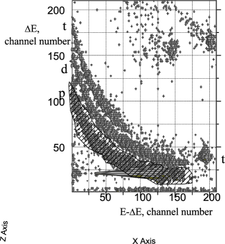
Fig. 1.: Particle distributions in the ($\Delta E-E$)-plane related to the telescope placed at $\Theta_{R2}=27.5^{\circ}$ (the right-hand side) with respect to the beam axis direction.  The locus, composed from the detected protons, is marked by a dark area

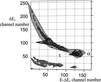
Fig. 2.: The same as in Fig.  1 but for the position of the telescope at $\Theta_{L2}=15^{\circ}$ (the left-hand side).  The locus, composed from the detected $\alpha$-particles, is marked by a dark area

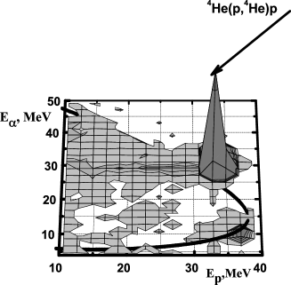
Fig. 3.: Two-dimensional spectra of the $p\alpha$-coincidences determined in the reactions ³H$\left(\alpha,p\alpha\right)2n$ at $E_{\alpha}=67.2$ MeV.  Arrow points to events of the elastic ⁴He$+p$ scattering due to hydrogen impurities in a T-Ti target

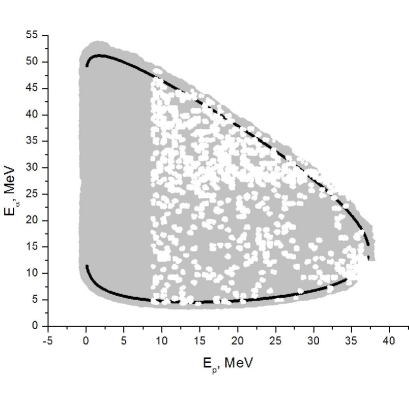
Fig. 4.: Selected experimental two-dimensional spectrum of the $p\alpha$-coincidence (white dots) and corresponding kinematical calculations

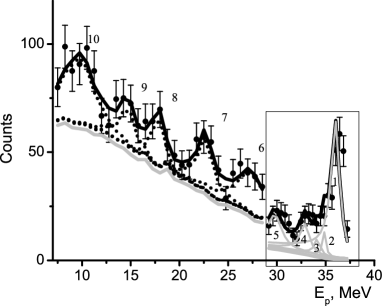
Fig. 5.: Resonance structure of ⁶He discovered in the reaction ³H$(\alpha,p\alpha)2n$.  The proton energy $E_{p}$ determined from the two-dimensional spectra of $p\alpha$-coincidences is projected on the excitation energy of ⁶He.  The results of approximation represented by expression (1) are plotted by black solid lines.  The contributions of different excited levels of ⁶He are marked by numbers 1–10 and displayed by dashed lines.  The low-energy part of experimental data is shown in a frame

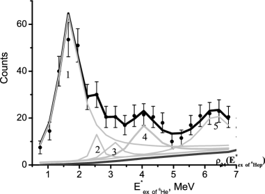
Fig. 6.: The same as in Fig.  5 but for the low-energy spectrum of ⁶He excitations

The further analysis consists in the selection of coincidence $p\alpha$-events from the four-body ³H$(\alpha,p\alpha)2n$ reaction in the measured two-dimensional $E_{p}\times E_{\alpha}$ spectrum.  It is well known that the $p\alpha$-coincidence events emerging from the four-body ³H$(\alpha,p\alpha)2n$ are disposed in parts of the represented spectrum, which are bounded by kinematic loci (see Fig. 3) and calculated for the hypothetical three-body ³H$(\alpha,p\alpha)\left\langle 2n\right\rangle$ reaction, where $\left\langle 2n\right\rangle$ is a particle consisting of two neutrons, which move in one direction with the energy of relative motion equal to zero [8]. The further analysis consists in the correct selection of these $p\alpha$-coincidence events.  First, by using the Monte Carlo simulation procedure [1,​ 9,​ 13] and by accounting for the real experimental conditions (the value of energy beam blurring, the dimensions of solid angles of detectors and beam spot), we determine a part of the ($E_{p}\times E_{\alpha}$) plane (Fig. 4, light grey background), in which the four-body experimental events can manifest themselves.  For each $i$-th light grey dot with $E_{\rm pkini}\times E_{\alpha{\rm kini}}$ coordinates with regard for the energy and momentum conservation laws [11,​ 12], we calculate the value $Q_{2-4{\rm kini}}$.  We use the Monte Carlo method for drawing the experimental $E_{p}\times E_{\alpha}$ spectrum (Fig. 3) and, for every obtained $E_{\rm piexp}\times E_{\alpha{\rm iexp}}$ event (see Fig. 4, white dots), determine the values $Q_{2-4{\rm expi}}$.  The criterion for selecting the necessary experimental events, which was formulated in [1], is used to extract them from the total array of experimental points.  The white dots in Fig. 4 are the selected experimental coincidence $p\alpha$-events obtained from the analysis of the four-body ³H$(\alpha,p\alpha)2n$ reaction.  More details about the implementation of the Monte Carlo procedure and the definitions of all input and output variables can be found in Ref. [9].  The white dots presented in Fig. 4 are the selected experimental coincidence $p\alpha$-events obtained as a result of the study of the four-body ³H$(\alpha,p\alpha)2n$ reaction.  In this figure, it is evident that the experimental events are cut at $E_{p}<10$ MeV, which is due to the use of $\Delta E$-detectors about 400 $\mu$m in thickness in the left telescope to detect and to identify protons. For the four-body reaction, resonances in two-body subsystems produce an increase in the intensity of break-up events in those places of the $E_{p}\times E_{\alpha}$ spectra, where the corresponding energy of the relative motion of decayed clusters achieves resonance energies.  We observed no resonance phenomenon caused by the $\alpha+p$ interaction in the obtained experimental data.  But before the analysis of two-dimensional $E_{p}\times E_{\alpha}$ spectra from the $\alpha+t$ interaction at $E_{\alpha}=27.2$ MeV [10], one can observed some bars filled by events, which are parallel to the alpha-particle energy axis, and these strips have been identified as a manifestation of the formation of the excited states in nucleus ⁶He and their subsequent decay by emitting three clusters $\alpha+n+n$.

Since we can explore the much higher excitation energy ($E_{\alpha}=67.2$ MeV) in this experiment, we hope for that this study will repeat the previous experiment and enhance our knowledge of the structure of the high-energy part of the excitation spectrum of ⁶He.  Indeed, in the spectrum (see Fig. 5) resulting from the projection of $p\alpha$-coincidence events of the four-body ³H$(\alpha,p\alpha)2n$ reaction (all white dots in the limits of the light grey background) on the proton energy axis, we can observe numerous resonant manifestations.  By our assumption, there are two possible mechanisms of this nuclear transformation – instantaneous formation of these four particles (so-called statistical model) and two-stage process of formation $p$, $\alpha$-particle, and two neutrons, in which a proton and ⁶He nucleus in one of the excited states are formed on the first stage.  On the second stage, the nucleus decays on three parts – $\alpha$-particle and two neutrons.  Then the yield of the four-body reaction can be calculated by a sum of the Breit–Wigner contributions with regard for the contribution of the simultaneous formation of proton, alpha-particle and two neutrons in the output channel of this reaction:

$$N\propto\rho_{24}\left(E_{p}\right)\!\sum_{j=1}^{k}\left[C_{j}\frac{\Gamma_{j}/2}{\left(E_{j}-E_{p}\right)^{2}+\left(\Gamma_{j}/2\right)^{2}}+B\right]\!,\!\!$$ (1)

where $\rho_{24}\left(E_{p}\right)$ is the projection of the phase space factor on the $E_{p}$ axis for the detection on coincidence of protons and alpha-particles from the four-body ³H$(\alpha,p\alpha)2n$ reaction; $C_{j}$ is the corresponding contribution of each unbound ⁶He^∗ state decaying into the $\alpha+n+n$ channel, and $B$ is the corresponding contribution due to the simultaneous formation of $p$, $\alpha,$ and two $n$.  The values of excitation energy of ⁶He and the phase space factor of the sequential three-body reaction, used in expression (1), are calculated with regard for the geometry and the energy parameters of the experiment and by using the Monte Carlo simulation.  The fitting procedure is carried out with the least-square method, and the quantities $E_{j}$, $\Gamma_{j}$, $C_{j},$ and $B$ were as variables.  The obtained energy parameters of ten excited levels from the fitting procedure are reported in Table 1.

Thus, we discovered ten excited levels of ⁶He (see also Fig. 5).  For each level, we determined the excitation energy and the width (see Table 1).  Most part of the discovered resonance states are narrow ones.  Their total width varies from $0.4\pm 0.2$ to $2.3\,\pm$ $\pm\,1.0$ MeV and is much less than the resonance energy measured from the three-cluster $\alpha+n+n$ threshold.

Table 1.: Excitation energy ($E$) and the width ($\Gamma$)
for the excited levels obtained in reactions generated
by the ³H${}+\alpha$ interaction.  Index $N_{s}$ numerates
excited levels in ⁶He.  $R1$ represents the reaction
³H${}+\alpha\rightarrow p+{}^{6}$He${}\rightarrow p+\alpha+n+n$ and $R2$ stands
for the reaction ³H${}+\alpha\rightarrow p+{}^{6}$He${}\rightarrow p+t+t$

$R1$, $E_{\alpha}=67.2$ MeV			$R1$, $E_{\alpha}=27.2$ MeV, [1]
$\Theta_{p}/\Theta_{\alpha}=27.5^{\circ}/$15.0∘			$\Theta_{p}/\Theta_{\alpha}=28.5^{\circ}/13.0^{\circ}\!\!+\!16.5^{\circ}\!\!+\!19.5^{\circ}$
$N_{s}$	$E$, MeV	$\Gamma$, MeV	$N_{s}$	$E$, MeV	$\Gamma$, MeV
1	$1.7\pm 0.2$	$0.65\pm 0.15$	1	$1.8\pm 0.2$	$0.3\pm 0.15$
2	$2.5\pm 0.2$	$0.4\pm 0.2$	2	$2.4\pm 0.2$	$0.4\pm 0.2$
3	$3.1\pm 0.3$	$0.4\pm 0.2$	3	$3.0\pm 0.2$	$0.6\pm 0.2$
4	$4.1\pm 0.3$	$0.9\pm 0.3$	$R2$, $E_{\alpha}=67.2$ MeV, [13]
5	$6.1\pm 0.3$	$1.6\pm 0.3$	10	$18.3\pm 0.2$	$0.0\pm 0.2$
6	$8.8\pm 0.4$	$2.0\pm 0.6$	$R2$, $E_{\alpha}=67.2$ MeV, [13]
7	$11.6\pm 0.4$	$2.0\pm 0.7$	$\Theta_{p}/\Theta_{t}=21.0^{\circ}/15.0^{\circ}$, 21.0${}^{\circ}/$20.0∘
8	$14.6\pm 0.4$	$2.3\pm 1.0$	8	$14.0\pm 0.4$	$0.6\pm 0.4$
9	$16.4\pm 0.4$	$1.4\pm 0.9$	9	$16.1\pm 0.4$	$0.8\pm 0.4$
10	$18.5\pm 0.4$	$1.7\pm 0.6$	10	$18.4\pm 0.4$	$1.0\pm 0.4$

Note that, in our experiments, we discovered quite new resonance states in ⁶He and confirmed the existence of some resonance states, which have been observed in other experiments.  For instance, the energy parameters of the observed excited states, marked as $N_{s}=2$ and $N_{s}=3$, almost coincide within experimental errors with the results of research at the cyclotron U-120 [1].  The excited level broader than our $N_{s}=2$ state was observed recently in the experiment using a beam of radioactive nuclei ⁸He [10].  The excited states with energy parameters close to those of our levels $N_{s}=8$, $N_{s}=9,$ and $N_{s}=10$ were observed in the inclusive deuteron spectra determined from the ⁷Li$(n,d)^{6}$He reaction [14] and from measurements of the $t-t$ and $p-t$ coincidence events in the ³H$(\alpha,tt)p$ and ³H$(\alpha,pt)t$ reactions [13].  The energy parameters of our $N_{s}=4$ excited state are close to the experimental values from Ref.  [15], where the excitation spectrum of ⁶He has been studied in the ⁶He$(p,p\alpha)$ reaction.  The resonances almost similar to our states $N_{s}=3$, 5, and 6 were observed in the experimental study of the ⁷Li$(t,\alpha)^{6}$He reaction [16], which is one of the first experiments devoted to the study of the excitation spectrum of ⁶He. Recently, Mougeot et al. [10]  observed two new resonance states.  The resonances with the parameters $E=2.6\pm 0.3$ MeV, $\Gamma=1.6\pm 0.4$ MeV, $J^{\pi}=2^{+}$ and $E=5.3\pm 0.3$ MeV, $\Gamma=2\pm 1$ MeV, $J=1$ were discovered in the transfer reaction $p\left({}^{8}{\rm He},t\right)$ induced by a beam of radioactive nuclei ⁸He.  As is seen, the energy of the first resonance state is very close to that of our $N_{s}=2$ state.  However, its width is much larger than that deduced in our experiments.  The second resonance state, discovered in [10], lies between our $N_{s}=4$ and $N_{s}=5$ states, not far from the $N_{s}=5$ state.

The comparison of different experimental methods demonstrates the consistency of our experimental results with results of other experimental investigations of the ⁶He resonance structure.

3 Theoretical Research

In this section, we briefly present the main ideas of a microscopic model formulated in Refs. [3,​ 17].  Note that a similar model was suggested in [18], which employs the generator coordinate method and was recently [19] used to study the resonances in ⁶He.

The present model is an extension of the resonating group method for the description of three-cluster systems.  It combines the $J$-matrix method or the algebraic version of the resonating group method with the hyperspherical harmonics (HH) method.  The former indicates that we use the full set of square integrable functions (namely, a specific set of three-cluster oscillator functions) to reduce the Schrödinger equation to that in the matrix form and to solve it.  It is well known that the hyperspherical harmonics method [3,​ 17,​ 20,​ 21,​ 22,​ 23,​ 4,​ 24] provides simple tools for imposing the suitable boundary conditions for the discrete and continuous spectra of three-cluster systems.

A microscopic model is based on two key elements: a Hamiltonian, which consists of the kinetic energy operator and the sum of pairwise nucleon-nucleon interactions, and a wave function.  The later determines, which part of the total Hilbert space is involved in the description of a many-particle system. That is why we start with a wave function of ⁶He.

In the present three-cluster model, the wave function of ⁶He can be written as

$$\Psi_{JM}=$$

$$=\sum_{SL}\widehat{\mathcal{A}}\left\{\left[\Phi_{1}\!\left(\alpha,b\right)\Phi_{2}\!\left(n\right)\Phi_{2}\!\left(n\right)\right]_{S}\phi_{L}\!\left(\mathbf{q}_{1},\mathbf{q}_{2}\right)\right\}_{JM}\!,\!\!\!$$ (2)

where $\Phi_{1}\left(\alpha,b\right)$ is an antisymmetric shell-model wave function describing the internal structure of the alpha-particle with four nucleons in the $s$-shell.  We indicate explicitly that the wave function of the alpha-particle $\Phi_{1}\left(\alpha,b\right)$, being an eigenfunction of the many-particle Hamiltonian with the harmonic oscillator interaction, depends on the oscillator length $b$, which is a variational parameter and has to be fixed (selected) in numerical calculations.  The neutron wave function $\Phi_{2}\left(n\right)$ only includes the spin and isospin variables of the neutron.  The quantity $\widehat{\mathcal{A}}$ stands for the total antisymmetrization operator, and the vectors $\mathbf{q}_{1}$ and $\mathbf{q}_{2}$ are the Jacobi vectors determining a relative position of clusters in the coordinate space.

The intercluster wave function $\phi_{L}\left(\mathbf{q}_{1},\mathbf{q}_{2}\right)$ of relative three-cluster motion is to be determined by solving the Schrödinger equation with the proper boundary conditions.  For this aim, we introduce the hyperspherical coordinates $q_{1}=\rho\sin\theta$ and $q_{2}=\rho\cos\theta$ and expand the wave function $\phi_{L}\left(\mathbf{q}_{1},\mathbf{q}_{2}\right)$ in the hyperspherical harmonic basis

$$\phi_{L}\left(\mathbf{q}_{1},\mathbf{q}_{2}\right)=\!\sum_{l_{1},l_{2}}\phi_{l_{1},l_{2};L}\!\left(\rho,\theta\right)\left\{Y_{l_{1}}\!\left(\widehat{\mathbf{q}}_{1}\right)Y_{l_{2}}\!\left(\widehat{\mathbf{q}}_{2}\right)\right\}_{LM}=$$

$$=\sum_{K,l_{1},l_{2}}\!\phi_{K;l_{1},l_{2};L}\!\left(\rho\right)\chi_{K}^{\left(l_{1},l_{2}\right)}\!\left(\theta\right)\left\{Y_{l_{1}}\!\left(\widehat{\mathbf{q}}_{1}\right)Y_{l_{2}}\!\left(\widehat{\mathbf{q}}_{2}\right)\right\}_{LM},$$ (3)

where $\widehat{\mathbf{q}}_{1}$ and $\widehat{\mathbf{q}}_{2}$ are the unit vectors.  The explicit form of the hyperspherical harmonics $\chi_{K}^{\left(l_{1},l_{2}\right)}\left(\theta\right)$ and the set of equations for hyperradial excitations $\phi_{K;l_{1},l_{2};L}\left(\rho\right)$ can be found in [3,​ 17,​ 4].

The hypermomentum $K$ and the partial angular momenta $l_{1}$ (along $\mathbf{q}_{1}$) and $l_{2}$ (along $\mathbf{q}_{2}$) define the three-cluster geometry and characterize the different scattering channels.  These three quantum numbers will be denoted as $c=\left\{K;l_{1},l_{2}\right\}$.   In the case where the total spin $S$ and the total orbital momentum $L$ of the compound system are not good quantum numbers (this takes place when, e.g., the spin-orbital components are presented in the nucleon-nucleon potential and are involved in calculations), five quantum numbers will numerate channels of the three-cluster system $c=\left\{K;l_{1},l_{2};LS\right\}$.  Within the present model, the total spin $S$ of ⁶He coincides with the spin of the two-neutron subsystem and may have two values $S=0$ and $S=1$.  The value $S=0$ is dominant, because it realizes a more stronger interaction between valence neutrons.  We recall that two neutrons with $S=0$ and the zero orbital momentum have a virtual state, which strongly enhances the cross section of elastic neutron-neutron scattering.

The hyperradial functions $\phi_{K;l_{1},l_{2};L}\left(\rho\right)$ at large values of $\rho$ have the asymptotic form

$$\phi_{K;l_{1},l_{2};L}\left(\rho\right)=\phi_{c;L}\left(\rho\right)\simeq$$

$$\simeq\delta_{c_{0},c}\psi_{c}^{\left(-\right)}\left(k\rho\right)-S_{c_{0},c}\psi_{c}^{\left(+\right)}\left(k\rho\right),$$ (4)

where $c_{0}$ denotes the incoming channel, $S_{c_{0},c}$ is an element of the many-channel $S$-matrix, and $\psi_{c}^{\left(+\right)}\!\left(k\rho\right)$ ($\psi_{c}^{\left(-\right)}\!\left(k\rho\right)$) is the incoming (outgoing) wave.  (The definitions of the wave functions $\psi_{c}^{\left(+\right)}\left(k\rho\right)$ and $\psi_{c}^{\left(-\right)}\left(k\rho\right)$ can be found in [3]).  Equation (4) shows explicitly the boundary conditions for the wave function of three-cluster continuous spectrum states.  These boundary conditions are implemented in the system of equations for the channel functions $\phi_{K;l_{1},l_{2};L}\left(\rho\right)$.  By solving these system, we obtain the wave functions of the three-cluster continuum and the $S$-matrix, which describe all kinds of elastic and inelastic processes in the compound system.

For the numerical calculation of properties of ⁶He, we make use of two effective NN-potentials: the Volkov (VP) [25] and Minnesota potentials (MP) [26].  These two potentials are frequently used in various microscopic models for investigating the light atomic nuclei (⁶He, in particular).  The Volkov potential contains only central components of the $NN$ interaction, and, thus, the total spin $S$ and the total orbital momentum $L$ are quantum numbers, as both $S$ and $L$ are the integrals of motion.  For this potential, we consider only one value of total spin $S=0$.  Since the Minnesota potential contains spin-orbital components (we took the IV-th version of the spin-orbital forces from Ref. [27]), the total spin $S$  and the total orbital momentum $L$ are no longer good quantum numbers.  Thus, the total angular momentum $J$ in the general case can be presented by a combination of four states  ($L,S$) with different values of the total spin $S$ and the total angular momentum $L$:

$$\left|J\right\rangle=\left|\left(J,0\right)\right\rangle+\left|\left(J-1,1\right)\right\rangle+\left|\left(J,1\right)\right\rangle+\left|\left(J+1,1\right)\right\rangle\!.$$

For $J^{\pi}=0^{+}$ and $J^{\pi}=1^{-}$ angular momenta, we have the following combination: $\left|0^{+}\right\rangle=\left|\left(0,0\right)\right\rangle+\left|\left(1,1\right)\right\rangle$ and $\left|1^{-}\right\rangle=\left|\left(1,0\right)\right\rangle+\left|\left(1,1\right)\right\rangle+\left|\left(2,1\right)\right\rangle$.

In the present model, we have got several input parameters such as the oscillator radius (or length) $b$ and the maximal value of hypermomentum $K_{\max}$ (which determines the maximal number of channels of the three-cluster continuum).  We select the oscillator length to minimize the alpha-particle energy.  For the Volkov and Minnesota potentials, this can be achieved with $b=1.37$ fm and $b=1.285$ fm, respectively.  For positive parity states, we take $K_{\max}=14.$ For negative parity states, we involve all hyperspherical harmonics up to $K_{\max}=13$.  Such set of hyperspherical harmonics provides stable results for the energy and the width of resonance states (see details in [17,​ 28]).  It was demonstrated in [28] that these hyperspherical harmonics account for the numerous scenarios of the decay of the three-cluster system.  We will use a large space of hyperradial excitations $n_{\rho.\max}=70$, which is equivalent to 140$\hbar\Omega$ excitations in the shell model.  This value of $n_{\rho.\max}$ is sufficiently large to provide the correct description of the internal part of the three-cluster wave function and to reach the asymptotic region.

We start our investigation with the calculation of the ground-state energy.  In Table 2, we display the ground-state energy of ⁶He and the parameters $m$ and $u$ for the Volkov and Minnesota potentials, respectively.  In Table 2, we also indicated the values of oscillator length $b$.

Table 2.: Input parameters, adjustable
parameters of the potential, and bound
state energy of ⁶He

Potential	VP N1	VP N2	VP N2	MP	Exp
$b$, fm	1.37	1.37	1.37	1.285	$-$
Parameter	$m=0.60$	$m=0.60$	$m=0.615$	$u=0.98$	$-$
$E$, MeV	$-1.387$	$-1.234$	$-0.953$	$-0.551$	$-0.973$

One can see that the Volkov potentials N1 and N2 with the original value of Majorana parameter $m=0.60$ overbound the ground state of ⁶He; whereas the Minnesota potential with the parameter $u=0.98$, which provides a correct description of the $\alpha+n$ subsystem, underbound the ground state of ⁶He.  The same values of parameter $u$ and oscillator radius $b$ were used in Refs. [29] to study the bound states of ⁶He, ⁶Li, and resonance states in ⁶He, ⁶Li, and ⁶Be within the complex scaling method.  For the Volkov potential N2, we found the value of Majorana parameter ($m=0.615$), which gives the proper ground-state energy.

By solving the system of dynamic equations, we obtain the scattering S-matrix $\left\|S_{cc^{\prime}}\right\|$ for the $N_{\rm ch}$ channel system and the $N_{\rm ch}$ wave functions.  The element $S_{c_{,}c^{\prime}}$ of the $S$-matrix describes the transition from the initial channel $c$ to the final channel $c^{\prime}$.  To analyze the states of the three-cluster continuum and transitions in the continuum, we use two different representations of the $S$-matrix.  In the first representation, we determine the inelastic parameter $\eta_{c_{,}c^{\prime}}$ and the corresponding phase shift $\delta_{c_{,}c^{\prime}}$

$$S_{c_{,}c^{\prime}}=\eta_{c_{,}c^{\prime}}\exp\left\{\!2i\delta_{c_{,}c^{\prime}}\!\right\}\!.$$ (5)

This is the traditional representation for the many-channel systems.  In the second representation, we deal with the uncoupled eigenchannels, each of them is determined by the eigenphase shift $\delta_{\nu}$ or the $S_{\nu}$-matrix

$$S_{\nu}=\exp\left\{2i\delta_{\nu}\right\}\!,$$ (6)

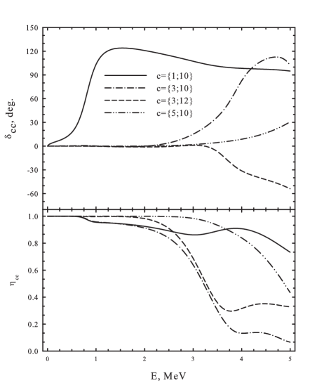
Fig. 7.: Phase shifts and inelastic parameters for four dominant channels in the $1^{-}$ state of ⁶He

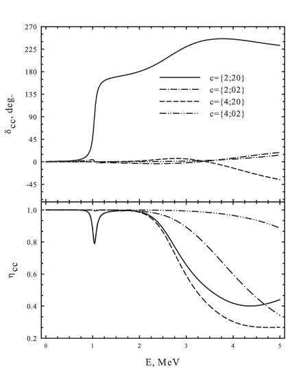
Fig. 8.: Phase shifts and inelastic parameters of the $2^{+}$ state as a function of the energy

where $\nu$ ($=1$, 2, …, $N_{\rm ch}$) numerates eigenchannels.  The relation between the original $\left\|S_{c_{,}c^{\prime}}\right\|$ and diagonal $\left\|S_{\nu}\right\|$ forms of the $S$- matrix is

$$S_{c_{,}c^{\prime}}=\sum_{\nu}U_{\nu}^{c}S_{\nu}U_{\nu}^{c^{\prime}},$$ (7)

where $\left\|U_{\nu}^{c}\right\|$ is an orthogonal matrix.  The energy and the width of a resonance state are determined from the eigenphase shift:

$$\left.\frac{d^{2}\delta_{\nu}}{dE^{2}}\right|_{E=E_{R}}=0,\quad\Gamma=2\left[\left.\frac{d\delta_{\nu}}{dE}\right|_{E=E_{R}}\right]^{-1}\!.$$

Our experience says (see, e.g., [28,​ 4]) that the resonance states of a three-cluster system usually manifest themselves in one specific eigenchannel.

We now turn our attention to the scattering parameters ($\delta_{c_{,}c^{\prime}}$, $\eta_{c_{,}c^{\prime}}$) and the parameters of resonances ($E$, $\Gamma$).  In Fig. 7, we display the phase shifts and the inelastic parameters for the diagonal elements of the $S$-matrix for the $J^{\pi}=1^{-}$ state.  These parameters are obtained with the VP N2 ($m=0.615$).  One can see a resonance behavior of the phase shift connected with the first channel $c_{1}=\left\{K=1,l_{1}=1,l_{2}=0\right\}$ at the energy around 1 MeV.  In this energy region, the inelastic parameters show a small probability of the inelastic processes.  The second resonance state is observed around 4 MeV and mainly connected with the second channel $c_{2}=\left\{K=3,l_{1}=1,l_{2}=0\right\}$.

In Fig.  8, we show the phase shifts and the inelastic parameters for the $2^{+}$ scattering state.

The well-known $2^{+}$ resonance state realizes itself as a classical Breit–Wigner resonance state in a few-channel system.  It displays itself in the phase shift associated with the channel {2,20}.  In the phase shift connected with the channel {2,02}, it is realized as a shadow resonance state.  The inelastic parameters connected with both dominant channels have a minimum at the resonance energy.  The second wide $2^{+}$ resonance state involves more channels.  Around this resonance, the strong rearrangements of compound nuclei are observed, which is confirmed by the behavior of the inelastic parameters $\eta_{cc}$.

There are many contradictory results in the literature about the $1^{-}$ resonance state.  The complex scaling method (CSM) [29,​ 30] and the hyperspherical harmonics method [31] considering ⁴He as a structureless particle do not confirm the existence of the state.  In Ref.  [32] within a new version of CSM, the $1^{-}$ state was obtained as a very broad resonance ($E=3.0$ MeV, $\Gamma=31.2$ MeV), which is hard to be detected experimentally.  In our model, we obtain the narrow $1^{-}$ state for the Volkov N1 and N2 potentials, and a wide resonance state for the Minnesota potential.  Let us consider the evolution of the state by increasing the space of hyperspherical harmonics.  We start our calculations with the simple case of $K_{\max}=1$.  Then we use $K_{\max}=3$, 5 and so on up to $K_{\max}=13$.  The results of these calculations, performed with the Volkov N2 potential ($m=0.615$) and the Minnesota potential ($u=0.98$), are displayed in Table 3.

One sees that there is no $1^{-}$ resonance state, when we use the hyperspherical harmonics with $K_{\max}=1$. When we involve all hyperspherical harmonics with $1\leq K\leq 3$, $1\leq K\leq 5$, and $1\leq K\leq 7$, we obtain a broad resonance state, where the total width of the resonance is larger than its energy.  We assume that it is very difficult to reveal such broad resonance state by other methods. Starting from $K_{\max}=9$, the $1^{-}$ resonance calculated with the Volkov potential turns out to be a narrow one.  However, for the Minnesota potential, the width of the $1^{-}$ resonance remains larger than its energy.  The results presented in Table 3 can explain why the $1^{-}$ resonance state was not observed in some calculations, for instance, in the CSM. When we use a part of the total Hilbert space $K_{\max}=3$, we impose a restriction on the possible values of partial orbital momenta $l_{1},l_{2}$: $1\leq l_{1}+l_{2}\leq 3$.  We assume that this restriction is crucial for the formation of the $1^{-}$ resonance state.  By enlarging the space of hyperspherical harmonics with $K_{\max}\geq 9$, we use a larger number of channels with $1\leq l_{1}+l_{2}\leq K_{\max}$.  This allows us to describe more correctly the internal part of the resonance wave function and its asymptotic part responsible for the decay of the resonance state.  By closing the discussion about the $1^{-}$ resonance state, we note that, within a similar three-cluster model [19], which combines the hyperspherical harmonics formalism with the generator coordinate method, the broad $1^{-}$ resonance state was obtained (the energy and the width of the resonance state are not specified).  This result, which was obtained with the Minnesota potential, partially coincides with our results (see Table 5).  Indeed, with the Minnesota potential, the width of the $1^{-}$ resonance is much larger than that of the resonance calculated with the Volkov potential.

Table 3.: Convergence of the energy
and the width (both in MeV) of the $1^{-}$ resonance state

	$K_{\max}$	1	3	5	7	9	11	13
VP	$E$	–	1.697	1.527	1.292	1.043	0.911	0.815
N2	$\Gamma$	–	2.996	2.022	1.311	0.788	0.585	0.460
MP	$E$	–	2.274	2.250	2.142	1.945	1.871	1.775
	$\Gamma$	–	6.399	4.665	3.577	2.476	2.116	1.780

Table 4.: Contribution of different states
with the total orbital momentum $L$ and the total
spin $S$ to the energy and the width
of the $1^{-}$ resonances in ⁶He

$(LS)$	(10)	$(10)+(11)$	$(10)+(11)+(21)$
$E$, MeV	1.842	1.776	1.775
$\Gamma$, MeV	2.750	1.783	1.780
$E$, MeV	3.892	3.222	3.264
$\Gamma$, MeV	3.597	3.698	3.635

Table 5.: Spectrum of resonance states
in ⁶He obtained with different $NN$ potentials.
Energy $E$ and width $\Gamma$ are in MeV

	VP N1		VP N2		VP N2		MP
	$m=0.60$		$m=0.60$		$m=0.615$		$u=0.98$
$J^{\pi}$	$E$	$\Gamma$	$E$	$\Gamma$	$E$	$\Gamma$	$E$	$\Gamma$	$J^{\pi}$
$0^{+}$	0.0	–	0.0	–	0.0	–	0.0	–	$0^{+}$
$1^{-}$	1.80	0.65	2.02	0.43	1.79	0.47	1.03	1 keV	$2^{+}$
$2^{+}$	2.01	0.15	2.10	0.05	2.01	0.11	2.32	1.63	$1^{-}$
$0^{+}$	2.25	1.98	2.506	1.71	2.34	1.87	3.10	1.04	$2^{+}$
$2^{+}$	3.54	1.96	3.64	1.80	3.56	1.74	3.12	1.29	$2^{-}$
$1^{-}$	4.21	2.41	4.44	2.00	4.26	2.18	3.59	1.87	$1^{+}$
$2^{-}$	5.09	4.97	7.03	5.25	5.30	5.40	3.65	3.34	$0^{+}$
$1^{+}$	5.13	2.59	5.37	2.24	5.20	2.50	3.77	3.76	$1^{-}$
							5.20	2.51	$1^{+}$

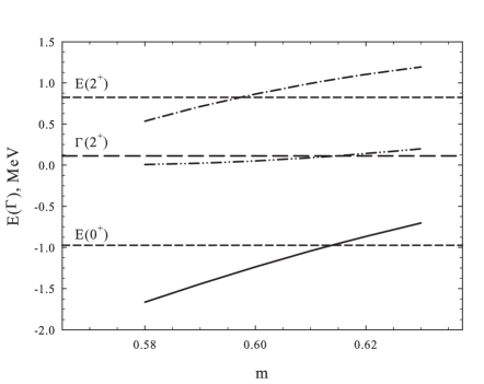
Fig. 9.: Energy of the ground state (solid line), energy (dash-dotted line) and width (dash-dot-dotted line) of $2^{+}$ resonance state as functions of the Majorana parameter $m$ (VP N2).  Experimental values of these quantities are indicated by dashed line

In Table 4, we show how the contributions of different values of the total orbital momentum $L$, total spin $S,$ and spin-orbital components of the Minnesota potential affect the parameters of the first and second $1^{-}$ resonance states.  The results presented in Table 4 can shed some more light on the problem of existence of the $1^{-}$ resonance state in ⁶He.  If we restrict ourselves with the total spin $S=0$ and thus switch-off the spin-orbital components of the Minnesota potential, we obtain a very wide resonance state.  By adding the component $(LS)=(11)$ to the total wave function, we slightly decrease the energy of the first $1^{-}$ resonance state and significantly reduce its width.  The next component $(LS)=(21)$ does not change the parameters of the resonance.  Thus, the first $1^{-}$ resonance state remains a wide resonance state, which, we believe, is difficult to be determined by the complex scaling method or other methods.  Note that the second resonance state became wider, as we increase the space of $(LS)$ components.  Indeed, the energy of the state is decreased, while the total width remains the same.

In Table 5, we display the spectrum of resonance states in ⁶He obtained with different $NN$ potentials.  The energy of resonances is reckoned from the ground-state energy.  The total angular momenta of resonance states for the Volkov potential are indicated on left-hand side of the table, while, for the Minnesota potential, they are shown on the right-hand side of the table.  We note that the Volkov potentials N1 and N2 yield a similar set of resonance states.  Moreover, the Volkov potential N1 and N2 generate the narrow $1^{-}$ resonance state.  The resonance width is between 0.473 and 0.647 MeV, and its energy is less than the energy of the well-known $2^{+}$ resonance state.  The latter is obtained with an energy of 2.012–2.096 MeV, which is $\approx 300$ keV larger than the experimental energy.  Contrary to the Volkov potential, the Minnesota potential creates a very narrow $2^{+}$ resonance state ($\Gamma$=1.0 keV) with an energy of 1.033 MeV, which is much less than the experimental value.  As is seen, the $0^{+}$ and $2^{-}$ resonance states, calculated with the Volkov N2 potential, are too broad.  So, it is very difficult to detect experimentally such short-living states.

We found that, with the selected $NN$ potentials, it is impossible to obtain simultaneously the correct values of energies of the $0^{+}$ bound state and the $2^{+}$ resonance state (with respect to the energy of the three-cluster threshold).  This statement is valid for the present model.  However, we believe that they can be obtained in other alternative models.  This statement is demonstrated in Fig.  9, where we display the the dependence of energy of the bound and $2^{+}$ resonance states on the Majorana parameter of the VP.  Note that this parameter is used in many microscopic calculations as a variational parameter.  In the cluster model or the resonating group method, the Majorana parameter is selected to reproduce the main properties of two-cluster subsystems of the compound three-cluster system.  One can also see that the relative position of the $0^{+}$ and $2^{+}$ states slightly changes with a variation of the Majorana parameter.  In addition, the optimal parameter $m$ for the $0^{+}$ state (where the energy coincides with the experimental one) differs from the optimal value $m$ for the $2^{+}$ resonance state and its width.  A similar picture is observed for the Minnesota potential (see Fig.  10).  The $2^{+}$ resonance state width obtained with the MP is very small with respect to the experimental value and is slightly changing in the displayed range of the parameter $u$.

Now we determine the dominant channels for the decay of resonances.  For this aim, we calculate the partial widths of resonance states.  In Table 6, we display the partial widths for resonances in ⁶He calculated with the Volkov potential N2.  Below each partial width $\Gamma_{\alpha}$ ($\alpha=1,2,...$), we also indicate the quantum numbers of channels $c_{\alpha}=$($K;l_{1}l_{2};LS$), into which a resonance state decays.  One notices that we display only three partial widths.  We show only dominant decay channels for a resonance state.  The total contribution of these channels to the total widths is at least 96%.  Thus, the contribution of the omitted channels is very small.

Let us analyze the quantum numbers of the dominant decay channels.  One can see, for example, that the first $2^{+}$ resonance state decays mainly through the channel with hypermomentum $K=2$ and with the zero value of orbital momentum of two valence neutrons.  Two dominant channels represent the decay of the second $2^{+}$ resonance state.  The first of them exhausts approximately 73% of the total width, while the second channel exhausts approximately 25%.  One also observes that all resonance states displayed in Table 6 have one or at most two dominant channels. Similar results are obtained with other NN-potentials.

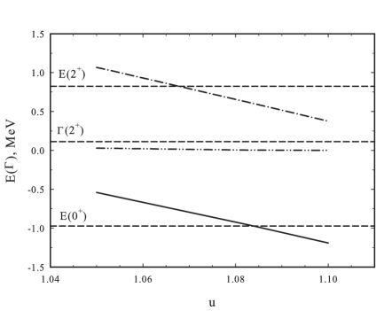
Fig. 10.: Energy of $0^{+}$ bound state, energy and width of the $\ 2^{+}$ resonance as a function of parameter $u$ of the MP

Table 6.: Total $\Gamma$ and partial $\Gamma_{i}$ ($i=1$, 2, 3)
widths for resonance states in ⁶He calculated
with the VP N2, $m=0.615$

$J^{\pi}$	$E$, MeV	$\Gamma$, MeV	$\Gamma_{1}/c_{1}$	$\Gamma_{2}/c_{2}$	$\Gamma_{3}/c_{3}$
$2^{+}$	1.033	0.107	0.096	0.011	0.0003
		($K;l_{1}l_{2};LS$)	(2;20;20)	(2;02;20)	(4;20;20)
$1^{-}$	0.808	0.473	0.466	0.006	0.0006
		($K;l_{1}l_{2};LS$)	(1;10;10)	(3;10;10)	(3;12;10)
$0^{+}$	1.364	1.869	1.028	0.830
			(0;00;00)	(2;00;00)
$2^{+}$	2.581	1.735	1.274	0.023	0.429
		($K;l_{1}l_{2};LS$)	(2;20;20)	(2;02;20)	(4;20;20)
$2^{-}$	4.317	5.399	4.930	0.001	0.442
			(3;12;20)	(3;21;20)	(3;01;20)
$1^{+}$	4.170	2.370	2.356	0.013	0.012
			(4;22;10)	(4;31;10)	(4;13;10)
$1^{-}$	3.284	2.184	0.183	1.186	0.690
			(1;10;10)	(3;10;10)	(3;12;10)

Here, we present the correlation functions in the coordinate and momentum spaces.  The definitions of these quantities are given in [33].  The correlation functions allow one to determine the most probable geometrical configuration of a three-cluster system.  This can be done both for the bound and resonance states.  In Ref.  [33], we formulated an algorithm of selecting the ‘‘true’’ resonance function among a large number of wave functions of the many-channel system. The algorithm allows us to analyze only one function or only one correlation function connected with the selected resonance state.

In Fig.  11, we display the correlation function for the first $1^{-}$ resonance state.  Figure 12 shows the correlation function for the first $2^{+}$ resonance state.

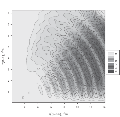
Fig. 11.: Correlation function for the $1^{-}$ resonance state calculated with the MP

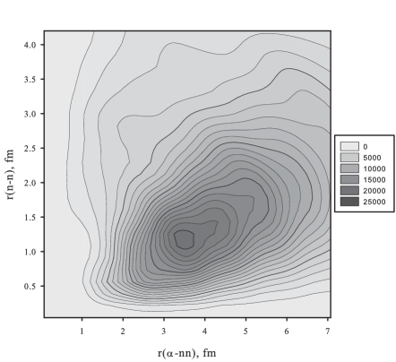
Fig. 12.: Correlation function for the first $2^{+}$ resonance state calculated with the Minnesota potential

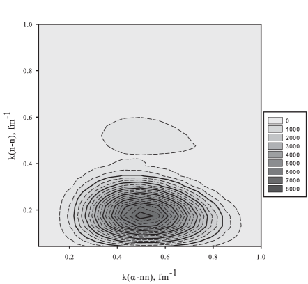
Fig. 13.: Correlation function for the $1^{-}$ resonance state calculated with the MP in the momentum space

One sees the common feature of these figures: a small distance between valence neutrons $r\left(n-n\right)$ and a large distance between the alpha-particle and the center of masses of the two-neutron subsystem $r\left(\alpha-nn\right)$.  Thus, the dominant configuration of ⁶He in these two resonances is an obtuse triangle.  The correlation function of the very narrow $2^{+}$ resonance state behaves itself as the correlation functions of a bound state.  This is the common feature of very narrow resonance states, which have the wave function very close to wave functions of quasibound states with the same energy.

The additional information about the three-cluster resonance state can be obtained by analyzing its correlation function in the momentum space.  In Figs.  13 and 14, we display the correlation functions of the $1^{-}$ and $2^{+}$ resonance states, respectively.  Both pictures were obtained with the Minnesota potential.  The main feature of the correlation functions is that the alpha particle has a larger relative momentum $k\left(\alpha-nn\right)$ than the relative momentum of two valence neutrons $k\left(n-n\right)$.

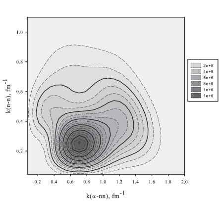
Fig. 14.: Correlation function determined in the momentum space with the MP for the first $2^{+}$ resonance state

To get a more information about the three-cluster resonance, we consider the decay cross section for a resonance state.  Having calculated elements of the scattering $S$-matrix, we can determine the cross sections of the elastic and rearrangement processes, which proceed in the three-cluster continuum.  Some examples of cross sections, which are determined by one hyperspherical harmonic, were demonstrated in [28].

It is well known (see, e.g., Refs.  [34,​ 35,​ 36,​ 37]) that the $3\Rightarrow 3$ scattering amplitude depends on 5 parameters ($\mathbf{k}_{0}$, $\mathbf{q}_{0}$) connected with the incoming channel and 5 parameters ($\mathbf{k}$, $\mathbf{q}$) attributed to the exit channel.  They are momenta associated with the Jacobi vectors.  In what follows, we determine the vector $\mathbf{k}$ as the momentum of the relative motion of a selected pair of clusters and the vector $\mathbf{q}$ as the momentum of motion of the third cluster with respect to the center of mass of the selected pair of clusters.  These vectors satisfy the relation

$$E=\frac{\hbar^{2}}{2m}\mathbf{k}_{0}^{2}+\frac{\hbar^{2}}{2m}\mathbf{q}_{0}^{2}=\frac{\hbar^{2}}{2m}\mathbf{k}^{2}+\frac{\hbar^{2}}{2m}\mathbf{q}^{2},$$ (8)

where $E$ is the total energy of the three-cluster system.  Thus, not all of the parameters are independent.  There are other relations, which reduce the number of independent parameters, if one needs to determine the $3\Rightarrow 3$ scattering amplitude.  We do not dwell on these relations.

In our case (in the representation of the hyperspherical harmonics), the amplitude is defined as

$$f\left(\mathbf{k}_{0},\mathbf{q}_{0};\mathbf{k},\mathbf{q}\right)=\sum_{K,l_{1},l_{2}}\sum_{\widetilde{K},\widetilde{l}_{1},\widetilde{l}_{2}}\sum_{M}\chi_{K}^{\left(l_{1},l_{2}\right)}\left(\theta_{0}\right)\times$$

$$\times\left(\delta_{K,l_{1},l_{2};\widetilde{K},\widetilde{l}_{1},\widetilde{l}_{2}}-S_{K,l_{1},l_{2};\widetilde{K},\widetilde{l}_{1},\widetilde{l}_{2}}\right)\chi_{\widetilde{K}}^{\left(\widetilde{l}_{1},\widetilde{l}_{2}\right)}\left(\theta\right)\times$$

$$\times\left\{Y_{l_{1}}\left(\mathbf{k}_{0}\right)Y_{l_{2}}\left(\mathbf{q}_{0}\right)\right\}_{LM}^{\ast}\left\{\!Y_{\widetilde{l}_{1}}\left(\mathbf{k}\right)Y_{\widetilde{l}_{2}}\left(\mathbf{q}\right)\!\right\}_{LM}\!.$$ (9)

The five-fold differential cross section describing rearrangements in the three-cluster continuum is

$$d\sigma\left(\mathbf{k}_{0},\mathbf{q}_{0};\mathbf{k},\mathbf{q}\right)\sim\left|f\left(\mathbf{k}_{0},\mathbf{q}_{0};\mathbf{k},\mathbf{q}\right)\right|^{2}d\mathbf{k}d\mathbf{q}.$$ (10)

One may define the amplitude $f_{c,\widetilde{c}}\left(\mathbf{k}_{0},\mathbf{q}_{0};\mathbf{k},\mathbf{q}\right)$ and the corresponding cross section $d\sigma_{c,\widetilde{c}}\left(\mathbf{k}_{0},\mathbf{q}_{0};\mathbf{k},\mathbf{q}\right)$ which determine the transition of the system from the three-cluster channel $c$ to the channel $\widetilde{c}$.  Let $\left|c\right\rangle$ be the hyperspherical harmonic

$$\left|c;\mathbf{k,q}\right\rangle=\left|K,l_{1},l_{2}\right\rangle=\chi_{K}^{\left(l_{1},l_{2}\right)}\left(\theta\right)\left\{Y_{l_{1}}\left(\mathbf{k}\right)Y_{l_{2}}\left(\mathbf{q}\right)\right\}_{LM}.$$ (11)

Then

$$f_{c,\widetilde{c}}\left(\mathbf{k}_{0},\mathbf{q}_{0};\mathbf{k},\mathbf{q}\right)\!=\!\left|c;\mathbf{k}_{0},\mathbf{q}_{0}\right\rangle\!\left[\delta_{c;\widetilde{c}}-S_{c;\widetilde{c}}\right]\left\langle\widetilde{c};\mathbf{k,q}\right|.\!$$ (12)

In view of Eq. (7) and the orthogonality properties of the matrix $\left\|U_{\nu}^{c}\right\|$, we can rewrite $f_{c,\widetilde{c}}\left(\mathbf{k}_{0},\mathbf{q}_{0};\mathbf{k},\mathbf{q}\right)$ as

$$f_{c,\widetilde{c}}\left(\mathbf{k}_{0},\mathbf{q}_{0};\mathbf{k},\mathbf{q}\right)=$$

$$=\left|c;\mathbf{k}_{0},\mathbf{q}_{0}\right\rangle\sum_{\nu}U_{\nu}^{c}\left[1\!-\!S_{\nu}\right]U_{\nu}^{\widetilde{c}}\left\langle\widetilde{c};\mathbf{k,q}\right|=$$

$$=\left|c;\mathbf{k}_{0},\mathbf{q}_{0}\right\rangle\sum_{\nu}U_{\nu}^{c}\left[1-S_{\nu}\right]U_{\nu}^{\widetilde{c}}\left\langle\widetilde{c};\mathbf{k,q}\right|.$$ (13)

This equation connects the eigenchannels $\nu$ with original channels $c$.

It is a very complicated and cumbersome tremendous expression to be analyzed and depends on too many input parameters.  We have to reduce the number of these parameters in order to get information in a simpler way.  If we integrate this many-fold cross section over the input parameters $\mathbf{k}_{0}$ and $\mathbf{q}_{0},$ we obtain

$$d\sigma\left(\mathbf{k},\mathbf{q}\right)\sim\left({\displaystyle\int}\left|f\left(\mathbf{k}_{0},\mathbf{q}_{0};\mathbf{k},\mathbf{q}\right)\right|^{2}d\mathbf{k}_{0}d\mathbf{q}_{0}\!\right)d\mathbf{k}d\mathbf{q}.$$

Thus, we obtain now the cross section, which is averaged over the input parameters or the initial conditions.  The new cross section $d\sigma\left(\mathbf{k},\mathbf{q}\right)$ depends on the parameters of exit channels and determines the decay of a three-cluster resonance state.  The expression for the cross section can be simplified by the integration over the unit vectors $\widehat{\mathbf{k}}$ and $\widehat{\mathbf{q}}$

$$d\sigma\left(k,q\right)\sim\left({\displaystyle\int}\sigma\left(\mathbf{k},\mathbf{q}\right)d\widehat{\mathbf{k}}d\widehat{\mathbf{q}}\right)dkdq.$$

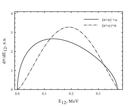
Fig. 15.: Differential cross section for the decay of the $2^{+}$ resonance state.  $E_{12}$ is the relative energy for a selected pair of clusters : the $n+n$ subsystem (solid line) and the $n+\alpha$ subsystem (dot-dashed line).  Results are obtained with the MP

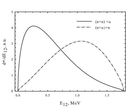
Fig. 16.: One-fold differential cross section, which determines the dominant energy and channels for the decay of the $1^{-}$ resonance state.  Results are obtained with the MP

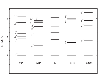
Fig. 17.: Comparison of the experimental ($E$) and theoretical (VP, MP, HH, CSM, see details in the text) spectra of resonance states in ⁶He.  Energy is reckoned from the ground state

In fact, the differential cross section $d\sigma\left(k,q\right)$ depends only on one parameter, because $k$ and $q$ are related by condition (8).  By introducing the energy of a selected pair of clusters $E_{12}=\frac{\hbar^{2}}{2m}k^{2}$, we can rewrite the expression for the differential cross section as

$$\frac{d\sigma\left(E_{12}\right)}{dE_{12}}\sim\left({\displaystyle\int}\sigma\left(\mathbf{k},\mathbf{q}\right)d\widehat{\mathbf{k}}d\widehat{\mathbf{q}}\right)\sqrt{E_{12}\left(1-E_{12}\right)}.$$ (14)

In Figs.  15 and 16, we display the cross sections (14) for the decay of the $2^{+}$ and $1^{-}$ resonance states calculated with the MP.  One can see that the $2^{+}$ resonance state prefers to decay, by emitting two neutrons with a small value ($E_{12}\approx 0.11$ MeV) of relative energy and the rather large energy ($E_{12}\approx 0.26$ MeV) of the alpha-particle (with respect to the center of mass of valence neutrons).  In other Jacobi coordinates, the resonance state selects an energy of approximately 0.2 MeV in the nucleon plus alpha-particle subsystem.  As for the $1^{-}$ resonance state, it also decays by emitting two neutrons with small relative energy ($E_{12}\approx 0.18$ MeV) and by emitting a neutron and an alpha particle with the relatively large value of energy ($E_{12}\approx 0.58$ MeV).  The channel $\left(n+\alpha\right)+n$ is dominant in the decay of the narrow $2^{+}$ resonance state, while the wide $1^{-}$ resonance state prefers to decay into the $\left(n+n\right)+\alpha$ channel.  This means, that our model predicts the sequential decay of the $2^{+}$ resonance state ${}^{6}{\rm He}\Rightarrow^{5}{\rm He}+n\Rightarrow\alpha+n+n$ and the simultaneous decay of the $1^{-}$ resonance state.

It is worth noting that the results for one-fold cross sections are in agreement with the results for the correlation functions (Figs. 11, 13, 12, and 14), which show the dominance of the small distance and the small relative momentum between the valence neutrons in the decay of the ⁶He three-cluster resonance states.

4 Experiment Versus Theory

In this section, we compare the experimental results with the results of some microscopic and semimicroscopic models.  In Fig. 17, we display the theoretical (MP, VP, HH, CSM) and experimental ($E$) spectra of resonance states in ⁶He.  As the theoretical results, we display the energy of resonance states calculated within our model with the Volkov potential N2, $m$=0.615, and the Minnesota potential.  These results are obtained in the present paper.  We also plotted the spectrum of resonance states calculated with the hyperspherical harmonics method [31] and with the CSM [38].  We selected those theoretical calculations, within which not only the well-known $2^{+}$ resonance state, but other states were discovered.  In Fig. 17, the symbol $E$ stands for the results of our experimental investigation with the beam energy $E_{\alpha}=67.2$ MeV.

It is obvious that the first experimental resonance state is the well-determined $2^{+}$ resonance.  There are two interpretations of the second experimental resonance state at $E=2.5\pm 0.2$ MeV. The calculations with the Minnesota potential suggest that this resonance states is the $J^{\pi}=1^{-}$ state, while our model with the Volkov potential proposes to interpret it as $J^{\pi}=0^{+}$ state.  Note that the HH and CSM methods have not revealed the resonance states with the energy close to $E=2.5\pm 0.2$ MeV.  One sees that the third resonance state ($E=3.1\pm 0.3$ MeV) may be interpreted as a combination of $2^{+}$ ($E=3.10$ MeV) and $2^{-}$ ($E=3.12$ MeV) resonance states, which are obtained with the MP.  The CSM yields the second $2^{+}$ resonance state with the energy $E=3.28$ MeV, which is close to the experimental value. However, there is no resonance states in the HH method with the energy around $E=3.1\pm 0.3$ MeV.  The resonance states calculated with the VP lie rather far from the energy $E=3.1\pm 0.3$ MeV. However, the $2^{+}$ resonance state with $E=3.56$ MeV may be connected with the third experimental resonance.  Our model indicates that the wide $1^{-}$ resonance states with the energy $E=4.26$ MeV (VP) and $E=3.77$ MeV (MP) may be attributed to the fourth experimental resonance state ($E=4.1\pm 0.3$ MeV).  As for other theoretical models, the HH model predicts two resonance $2^{+}$ and $1^{+}$ states, and the CSM does one $1^{+}$ resonance close to the fourth experimental state.  Concluding this section, we say that the results of a few theoretical models are in agreement with those of the present experimental methods.

5 Conclusion

We have considered the resonance structure of ⁶He.  Both the experimental and theoretical methods were used to investigate the parameters and the nature of resonance states of ⁶He.  For the experimental detection of ⁶He resonance states, the reaction ³H$(\alpha,p\alpha)2n$ with a four-body exit channel was used.  The reaction was induced by the interaction of alpha-particles (the energy of a beam $E_{\alpha}=67.2$ MeV) with tritons.  Information about the parameters of resonance states was obtained from the $p-\alpha$ coincidence spectra.  Ten resonance states were discovered.  The most part of these states are narrow resonances, as their total width is less than the energy of a resonance.

A microscopic model was exploited for the theoretical analysis of the discrete and continuum spectra in ⁶He.  This model incorporates the dominant three-cluster configuration $\alpha+n+n$ and involves the full set of oscillator functions enumerated by quantum numbers of the hyperspherical harmonics model to describe the relative motion of three interacting clusters.  A large set of hyperradial and hyperspherical excitations was used in calculations to provide with the stable and convergent results for the energies and the widths of the resonance states.  Two different effective $NN$ potentials were used to model the interaction between nucleons and to determine the interaction between valence neutrons and the alpha-particle.  We discovered the set of the $0^{+}$, $1^{-}$, $1^{+}$, and $2^{+}$ resonances.  The total and partial widths of these resonances were determined, and the dominant decay channels of the resonances were revealed.  We demonstrated that the resonance states are mainly formed by one or two channels of the three-cluster continuum.  These selected channels are weakly coupled to other channels, which predetermines the existence of resonance states in the many-channel system.

It was demonstrated that the results of the present microscopic model satisfactorily agree with the new experimental data.

О.М. Поворозник, В.С. Василевський
СПЕКТР РЕЗОНАНСНИХ СТАНIВ В ⁶He.
ЕКСПЕРИМЕНТАЛЬНИЙ ТА ТЕОРЕТИЧНИЙ АНАЛIЗ
Р е з ю м е
Вивчено структуру резонансних станiв в ⁶He експериментальними та теоретичними методами. Приведено результати експериментального дослiдження спектра трикластерного континууму ⁶He. Для цього залучено реакцiю ³H$(\alpha,p\alpha)nn$, яка генерується взаємодiєю альфа-частинок з тритiєм при енергiї пучка $E_{\alpha}=67{,}2$ MеВ. Теоретичний аналiз резонансної структури ⁶He проводиться в рамках трикластерної мiкроскопiчної моделi. Ця модель використовує гiперсферичнi гармонiки для опису динамiки вiдносного руху кластерiв. Набiр нових резонансних станiв знайдено експериментальним та теоретичним методами. Визначено енергiю, ширину та домiнуючi канали розпаду резонансiв. Отриманi результати детально порiвнюються iз результатами рiзних теоретичних моделей, а також експериментiв.

References

- [1] G. Mandaglio, O. Povoroznyk, O.K. Gorpinich, O.O. Jachmenjov, A. Anastasi, F. Curciarello, V. De Leo, H.V. Mokhnach, O. Ponkratenko, Y. Roznyuk, G. Fazio, and G. Giardina, Mod. Phys. Lett. A 29, 1450105 (2014).
- [2] O.K. Gorpinich, O.M. Povoroznyk, Y.S. Roznyuk, and B.G. Struzhko, Scientific papers KINR, Kiev, Ukraine, 3(50), 53 (2001).
- [3] V. Vasilevsky, A.V. Nesterov, F. Arickx, and J. Broeckhove, Phys. Rev. C 63, 034606 (2001).
- [4] A.V. Nesterov, F. Arickx, J. Broeckhove, and V.S. Vasilevsky, Phys. Part. Nucl. 41, 716 (2010).
- [5] A.I. Baz’, Soviet J. Exp. Theor. Phys. 43, 205 (1976).
- [6] V. Zerkin, V. Konfederatenko, O.M. Povoroznik, B.G. Struzhko, and A.M. Shydlyk, Preprint KINR, Kiev, Ukraine, 91–11, 1 (1991).
- [7] O. Povoroznyk, O.K. Gorpinich, O.O. Jachmenjov, H.V. Mokhnach, O. Ponkratenko, G. Mandaglio, F. Curciarello, V. De Leo, G. Fazio, and G. Giardina, J. Phys. Soc. Japan 80, 094204 (2011).
- [8] M. Furić and H.H. Forster, Nucl. Instr. Meth. 98, 301 (1972).
- [9] O. Povoroznyk, Nucl. Phys. Atom. Energy 8, 131 (2007).
- [10] X. Mougeot, V. Lapoux, W. Mittig, N. Alamanos, F. Auger, B. Avez, D. Beaumel, Y. Blumenfeld at el., Phys. Lett. B 718, 441 (2012).
- [11] S. Nakayama, T. Yamagata, H. Akimune, I. Daito, H. Fujimura, Y. Fujita, M. Fujiwara at el., Phys. Rev. Lett. 85, 262 (2000).
- [12] W.D.M. Rae, A.J. Cole, B.G. Harvey, and R.G. Stokstad, Phys. Rev. C 30, 158 (1984).
- [13] O.M. Povoroznyk, O.K. Gorpinich, O.O. Jachmenjov, H.V. Mokhnach, O. Ponkratenko, G. Mandaglio, F. Curciarello, V. De Leo, G. Fazio, and G. Giardina, Phys. Rev. C 85, 064330 (2012).
- [14] F.P. Brady, N.S.P. King, B.E. Bonner, M.W. McNaughton, J.C. Wang, and W.W. True, Phys. Rev. C 16, 31 (1977).
- [15] A. Lagoyannis, F. Auger, A. Musumarra, N. Alamanos, E.C. Pollacco, A. Pakou, Y. Blumenfeld, F. Braga at el., Phys. Lett. B 518, 27 (2001).
- [16] K.W. Allen, E. Almqvist, J.T. Dewan, and T.P. Pepper, Phys. Rev. 96, 684 (1954).
- [17] V. Vasilevsky, A.V. Nesterov, F. Arickx, and J. Broeckhove, Phys. Rev. C 63, 034607 (2001).
- [18] S. Korennov and P. Descouvemont, Nucl. Phys. A 740, 249 (2004).
- [19] A. Damman and P. Descouvemont, Phys. Rev. C, 80, 044310 (2009).
- [20] M.V. Zhukov, B.V. Danilin, D.V. Fedorov, J.M. Bang, I.J. Thompson, and J.S. Vaagen, Phys. Rep. 231, 151 (1993).
- [21] J.M. Bang, B.V. Danilin, V.D. Efros, J.S. Vaagen, M.V. Zhukov, and I.J. Thompson, Phys. Rep. 264, 27 (1996).
- [22] A. Cobis, D.V. Fedorov, and A.S. Jensen, Nucl. Phys. A 631, 793 (1998).
- [23] A. Cobis, D.V. Fedorov, and A.S. Jensen, Phys. Rev. C 58, 1403 (1998).
- [24] Y.A. Lurie and A.M. Shirokov, Ann. Phys. 312, 284 (2004).
- [25] A.B. Volkov, Nucl. Phys. 74, 33 (1965).
- [26] D.R. Thompson, M. LeMere, and Y.C. Tang, Nucl. Phys. A 286, 53 (1977).
- [27] I. Reichstein and Y.C. Tang, Nucl. Phys. A 158, 529 (1970).
- [28] V. Vasilevsky, A.V. Nesterov, F. Arickx, and J. Broeckhove, Phys. Rev. C 63, 064604 (2001).
- [29] A. Csótó, Phys. Rev. C 48, 165 (1993); 49, 2244 (1994); 49, 3035 (1994).
- [30] K. Arai, Y. Suzuki, and K. Varga, Phys. Rev. C 51, 2488 (1995).
- [31] B.V. Danilin, T. Rogde, S.N. Ershov, H. Heiberg-Andersen, J.S. Vaagen, I.J. Thompson, M.V. Zhukov, A. Sedrakian, T. Alm, and U. Lombardo, Phys. Rev. C 55, 577 (1997).
- [32] S. Aoyama, Phys. Rev. C 68, 034313 (2003).
- [33] J. Broeckhove, F. Arickx, P. Hellinckx, V.S. Vasilevsky, and A.V. Nesterov, J. Phys. G Nucl. Phys. 34, 1955 (2007).
- [34] E. Gerjuoy, Phil. Trans. Roy. Soc. Lond. A 270, 197 (1971).
- [35] R.G. Newton, Ann. Phys. 74, 324 (1972).
- [36] A.I. Baz and S.P. Merkurev, Theor. Math. Phys. 31, 309 (1977).
- [37] R.I. Jibuti and R.Y. Keserashvili, Czech. J. Phys. 30, 1090 (1980).
-
[38]
S. Aoyama, S. Mukai, K. Kato, and
K. Ikeda, Prog. Theor. Phys. 93, 99 (1995); 94,
343 (1995).
Received 18.07.14