Metric Localization using Google Street View

Abstract

Accurate metrical localization is one of the central challenges in mobile robotics. Many existing methods aim at localizing after building a map with the robot. In this paper, we present a novel approach that instead uses geotagged panoramas from the Google Street View as a source of global positioning. We model the problem of localization as a non-linear least squares estimation in two phases. The first estimates the 3D position of tracked feature points from short monocular camera sequences. The second computes the rigid body transformation between the Street View panoramas and the estimated points. The only input of this approach is a stream of monocular camera images and odometry estimates. We quantified the accuracy of the method by running the approach on a robotic platform in a parking lot by using visual fiducials as ground truth. Additionally, we applied the approach in the context of personal localization in a real urban scenario by using data from a Google Tango tablet.

I Introduction

Accurate metrical positioning is a key enabler for a set of crucial applications, from autonomous robot navigation, intelligent driving assistance to mobile robot localization systems. During the past years, the robotics and the computer vision community formulated accurate localization solutions that model the localization problem as pose estimation in a map generated with a robot. Given the importance of map building, researchers have devoted significant resources on building robust mapping methods [23, 6, 26, 12]. Unfortunately, localization based on maps built with robots still presents disadvantages. Firstly, it is time consuming and expensive to compute an accurate map. Secondly, the robot has to visit the environment beforehand. An alternative solution is to re-use maps for localization even if they were not designed for robots. If maps do not exist, we can use various robot mapping algorithms, but if maps exist and a robot can utilize them, it will allow the robot to navigate without needing to explore the full environment beforehand.

In this paper, we propose a novel approach that allows robots to localize with maps built for humans for the purpose of visualizing places. Our method does not require the construction of a new consistent map and nor does it require the robot to previously visit the environment. Our central idea is to leverage Google Street View as an abundant source of accurate geotagged imagery. In particular, our key contribution is to formulate localization as the problem of estimating the position of Street View’s panoramic imagery relative to monocular image sequences obtained from a moving camera. With our approach, we can leverage Google’s global panoramic image database, with data collected each 5-10m and continuously updated across five continents [9, 3]. To make this approach as general as possible, we only make use of a monocular camera and a metric odometry estimate, such as the one computed from IMUs or wheel encoders.

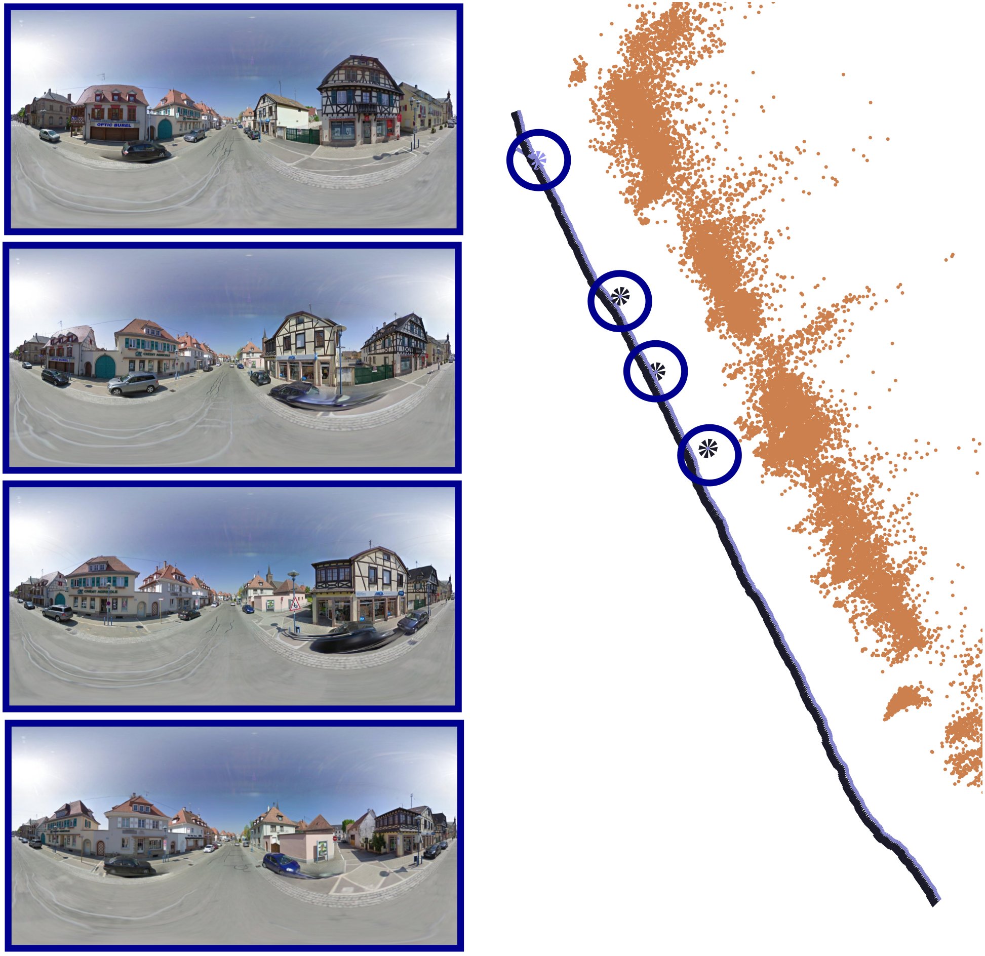
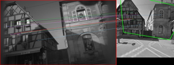
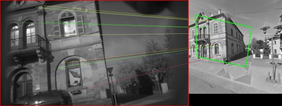
Figure 1: Localization of a moving camera from Street View panoramas. The location of the panoramas are 27 Rue du Mal Foch, Marckolsheim, France. Four panoramas shown in top-left are localized with respect to the camera trajectory (black) and estimated 3D points (orange). The bottom two images show feature matching between Tango images and rectilinear views of the panorama.

We formulate our approach as a non-linear least squares problem of two objectives. In the first, we estimate the 3D position of the points in the environment from a short monocular camera trajectory. The short trajectories are motivated by limiting the computation time, restricting the estimation problem and the presence of abundant panoramic imagery. In the second, we find panoramas that match the images and compute their 6DOF transformation with respect to the camera trajectory and the estimated 3D points. As the GPS coordinates of the panoramic images are known, we obtain estimates of the camera positions relative to the global GPS coordinates. Our aim is not to accurately model the environment or to compute loop closures for improving reconstruction. Our approach can be considered as a complement of GPS systems, which computes accurate positioning from Street View panoramas. For this reason, we tested our method on a Google Tango smartphone in two kinds of urban environments, a suburban neighborhood in Germany and a main road of a village in France. Additionally, we quantify the accuracy of our technique by running experiments in a large parking lot with ground truth computed from visual fiducials. In the experiments, we show that with our technique we are able to obtain submeter accuracy and robustly localize users or robots in urban environments.

II Related work

There exist previous literature about using Street View imagery in the context of robotics and computer vision. Majdik et al. [16] use Street View images to localize a Micro Aerial Vehicle by matching images acquired from air to Street View images. Their key contribution is matching images with strong view point changes by generating virtual affine views. Their method only solves a place recognition problem. We, on the other hand, compute a full 6DOF metrical localization on the panoramic images. In [17], they extended that work by adding 3D models of buildings as input to improve localization. Other researchers have matched Street View panoramas by matching descriptors computed directly on it [25]. They learn a distinctive bag-of-word model and use multiple panoramas to match the queried image. Those methods provide only topological localization via image matching. Related to this work is the topic of visual localization, which has a long history in computer vision and robotics, see [8] for a recent survey. Various approaches have been proposed to localize moving cameras or robots using visual inputs [4, 5, 2, 13, 24]. Our work is complimentary to such place recognition algorithms as these may serve as a starting point for our method. Topological localization or place recognition serves as a pre-processing step in our pipeline. We use a naive bag-of-words based approach, which we found to be sufficient for place recognition. Any of the above-mentioned methods can be used instead to make the place recognition more robust.

Authors have also looked into localizing images in large scale metrical maps built from structure-from-motion. Irschara et al. [10] build accurate point clouds using structure from motion and then compute the camera coordinates of the query image. In addition, they generate synthetic views from the dense point cloud to improve image registration. Zhang and Kosecka [29] triangulate the position of the query image by matching features with two or more geotagged images from a large database. The accuracy of their method depends on the density of the tagged database images. Sattler et al. [22] also localize query images in a 3D point cloud. Instead of using all the matching descriptors, they use a voting mechanism to detect robust matches. The voting scheme enables them to select 3D points which have support from many database images. This approach is further improved in  [21] by performing a search around matched 2D image features to 3D map features and vice versa. Zamir and Shah [27] build a dense map from 100,000 Google street view images and then localize query images by a GPS-tag-based pruning method. They provide a reliability score of the results by evaluating the kurtosis of the voting based matching function. In addition to localizing single images, they can also localize a non-sequential group of images.

Unlike others, our approach does not rely on accurate maps built with a large amount of overlapping geotagged images. As demonstrated by the experiments, our approach requires only a few panoramas for reliable metric localization with submeter accuracy.

III Method

Figure 2: Flowchart illustrating various modules in our pipeline.

In this section we outline the technical details for using Google’s Street View geotagged imagery as our map source for robot localization. Our goal is not to built large scale accurate maps. Instead, we want to approximately estimate the 3D position of the features relative to the camera positions and then compute the rigid body transformation between the Street View panoramas and the estimated points. This allows us to compute the GPS positions of the camera position in global GPS coordinates. Our current implementation works offline. The flowchart shown in Figure 2 illustrates the workflow between the various modules.

III-A Tracking Features in an Image Stream

The input of our method is an image stream acquired from a monocular camera. We define $\mathcal{S}=(s_{1},\ldots,s_{S})$ as a sequence of $S$ images. A sequence is implemented as a short queue that consists only of the last few hundreds frames acquired by the camera. An image $s_{i}$ is a 2D projection of the visible 3D world, through the lens, on a camera’s CCD sensor. For estimating the 3D position of the image points, we need to collect bearing observations from several positions as the camera moves.

We take a sparse features approach for tracking features in the stream of camera images. For each image $s_{i}$, we extract a set of keypoints computed by using state-of-the-art robust feature detectors, such as SIFT [15]. A description $d\in\mathcal{D}_{i}$ is computed from the image patch around each keypoint. $\mathcal{F}_{i}$ is the set of keypoints and descriptors and is denoted as the feature set.

Each time a new image arrives, we find feature correspondences between $s_{i}$ and $s_{i-1}$. We compute neighbor matches using FLANN [19] between all elements of $\mathcal{D}_{i}$ and $\mathcal{D}_{i-1}$. A match is considered valid if the distance to the best match is $0.7$ times closer than the second best [15]. As these correspondences only consider closeness in descriptor space, in addition we employ a homography constraint to consider the keypoint arrangement between two images. We use the keypoints of the matched descriptors for a RANSAC procedure that computes the inlier set for the perspective transformation between the two images. We call a track $\mathcal{T}_{j}$, the collection of all the matched keypoints relative to the same descriptor over the consecutive image frames $\mathcal{S}$. A track is terminated as soon as the feature cannot be matched in the current image. For an image stream $\mathcal{S}$, we collect the set of tracks $\mathcal{T}_{\mathcal{S}}$ consisting of the features $\mathcal{F}_{\mathcal{S}}$.

Note that tracks have different length. Some keypoints are seen from many views, while others are seen from few. Intuitively, long tracks are good candidates for accurate 3D point estimation as they have longer baselines. We only perform feature matching across sequential image frames. No effort is spent on matching images which are not sequential: this work does not make any assumption on the motion of the robot, on the visibility of the environment or on the existence of possible loops.

III-B Non-Linear Least Squares Optimization for 3D Point Estimation

First Optimization	Second Optimization

Figure 3: Optimization problem for estimating the position of the features, $\mathbf{y}$ shown as stars, and the camera positions $\mathbf{x}$ shown as frustums. The dotted lines represent bearing constraints while the solid black line represents the odometry constraint. The right image shows the optimization problem for computing the position of the panorama $\mathbf{p}$ from the computed 3D points.

The next step is to compute 3D points from the tracks $\mathcal{T}_{\mathcal{S}}$. In our system, we have rigid body odometric constraints between consecutive camera poses $\mathbf{x}_{i}$ and $\mathbf{x}_{i+1}$, associated to frame $s_{i}$ and $s_{i+1}$. Our method is agnostic to the kind of odometry: it can be computed by integrating IMUs, wheel encoders, or by employing an IMU-assisted visual odometry. In our problem formulation, we consider the monocular camera calibrated and all the intrinsic parameters known.

Each keypoint in track $\mathcal{T}_{j}$ corresponds to a 3D point $\mathbf{y}_{j}$ observed in one of the images with pixel coordinates $u$, $v$. If we consider a pinhole camera model, the camera matrix $\mathbf{C}$ projects a point $\mathbf{y}_{j}$ into the camera frame:

$$\mathbf{C} = \left[\begin{array}[]{ccc}f_{x}&0&c_{x}\\ 0&f_{y}&c_{y}\\ 0&0&1\end{array}\right]$$ (4)

The direction vector

$$\mathbf{d} = \mathbf{C}^{-1}[u,v,1]^{T},$$ (5)

can be interpreted as the direction of $\mathbf{y}_{j}$ with respect to the camera center. Then, we compute the elevation and bearing angles:

$$\theta = \operatorname{arccos}\left(\frac{d_{z}}{\sqrt{d^{2}_{x}+d^{2}_{y}+d^{2}_{z}}}\right)$$ (6)

$$\varphi = \operatorname{arctan}\left(\frac{d_{y}}{d_{x}}\right)$$ (7)

A least squares minimization problem can be described by the following equation:

$$\mathbf{F}(\mathbf{x},\mathbf{y}) = \sum_{ij}\mathbf{e}_{ij}(\mathbf{x},\mathbf{y})^{T}\mathbf{\Sigma}_{ij}\mathbf{e}_{ij}(\mathbf{x},\mathbf{y})$$ (8)

$$+ \sum_{k}\mathbf{e}_{k,k+1}(\mathbf{x})^{T}\mathbf{\Lambda}_{k}\mathbf{e}_{k,k+1}(\mathbf{x})$$

Here

• $\mathbf{x}=(\mathbf{x}_{1}^{T},\;\ldots\;,\mathbf{x}_{n}^{T})^{T}$ is a vector of monocular camera poses, where each $\mathbf{x}_{i}$ represents a 6DOF pose.

• $\mathbf{y}=(\mathbf{y}_{1}^{T},\;\ldots\;,\mathbf{y}_{m}^{T})^{T}$ is a vector of 3D points in the world associated to the tracked features.

• $\mathbf{e}_{ij}(\mathbf{x},\mathbf{y})$ is a vector error function that computes the distance between a measurement prediction $\mathbf{\hat{z}}_{ij}(\mathbf{x},\mathbf{y})$ and a real measurement $\mathbf{z}_{ij}=[\theta_{ij},\phi_{ij}]$. The error is $\mathbf{0}$ if $\mathbf{z}_{ij}=\hat{\mathbf{z}}_{ij}$, that is when the measurement predicted via $\mathbf{\hat{z}}_{ij}(\mathbf{x},\mathbf{y})$ from the states $\mathbf{x}_{i}$ and $\mathbf{y}_{j}$ is equal to the real measurement.

• $\mathbf{\hat{z}}_{ij}(\mathbf{x},\mathbf{y})$ computes the bearing and azimuthal angles from camera pose $\mathbf{x}_{i}$ to feature $\mathbf{y}_{j}$ in the camera frame.

• $\mathbf{\Sigma}_{ij}$ represents the information matrix of a measurement that depends on the state variables in $\mathbf{x}$.

• $\mathbf{e}_{k,k+1}(\mathbf{x})$ is a vector error from the predicted odometry measurements.

• $\mathbf{\Lambda}_{k}$ represent the information matrix of the odometry.

We initialize the camera position $\mathbf{x}$ with odometry and the feature positions $\mathbf{y}$ by triangulation. We employ the optimization framework g2o [14] as our non-linear least squares solver. First, we solve Eq. 8 by keeping $\mathbf{x}$ fixed:

$$\mathbf{y}^{*} = \mathop{\rm argmin}_{\mathbf{y}}\mathbf{F}(\mathbf{x},\mathbf{y})$$ (9)

This results in an improved estimation of $\mathbf{y}$. Second, we perform a full joint optimization of all the estimated 3D points $\mathbf{y}$ and camera poses $\mathbf{x}$.

$$(\mathbf{x}^{*},\mathbf{y}^{*}) = \mathop{\rm argmin}_{\mathbf{x},\mathbf{y}}\mathbf{F}(\mathbf{x},\mathbf{y})$$ (10)

The use of RANSAC helps improve the feature correspondences but does not guarantee an absence of outliers. Therefore, the robust methods developed in the previous chapters are used to improve the robustness against such errors. We use Dynamic Covariance Scaling kernel, a robust M-estimator to improve convergence and to handle wrong data associations [1].

Note that we are not aiming at an accurate reconstruction of the environment. In our approach, we only perform data association between sequential images as we do not compute loop closures or perform large baseline feature triangulation. There may be situations where a track is broken due to occlusions or changes in the viewpoint. We do not try to merge tracks in such scenarios. This is avoided for the process to be less computationally demanding. Doing a full bundle-adjustment will definitely help in a better reconstruction of the environment but that is not the goal of our work.

III-C Matching of Street View Panoramas with Camera Images

Google Street View can be considered as an online browsable dataset consisting of billions of street-level panoramic images acquired all around the world [9]. It is of key importance that each image is geotagged with a GPS position. This position is highly accurate and it is the result of a careful optimization at global-scale by Google [13]. In particular, Street View images are acquired by vehicles with a special apparatus consisting of cameras mounted around a spherical mounting. All camera images are stitched together to form a spherical panoramic image represented via a plate carrée projection. This results in a high quality image often exceeding 20M pixels resolution for each panorama.

Google provides public APIs for requesting virtual camera views of a given panorama. These views are rectilinear projection of the spherical panorama with a user selected field-of-view, orientation and elevation angle. Rectilinear views can be considered as undistorted images from a pinhole camera, free of distortion. A panorama can be selected via its GPS position or its ID. An example of a panorama acquired from Wall Street, New York, is illustrated in Figure 4. For robustness, we extract rectilinear horizontal overlapping images. The overlapping region aids in matching at image boundaries. We do not use the top and the bottom image as it often contains only sky and floor.

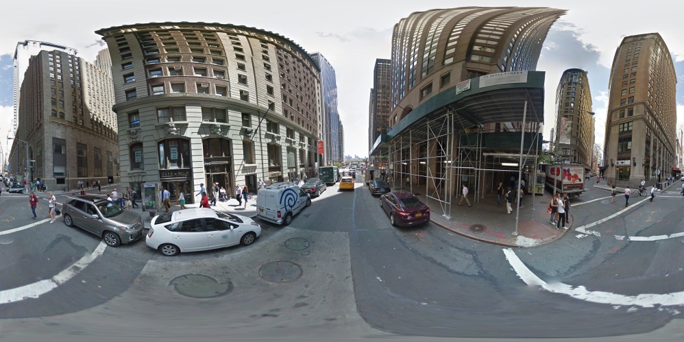
Figure 4: A panorama downloaded from Street View (top) with the extracted rectilinear views (bottom). Each image has a $90^{\circ}$ field-of-view. These are considered pinhole cameras, free of distortion and they overlap horizontally to aid matching across image boundaries.

In order to match panoramas with monocular camera trajectories we first need a candidate set of panoramas. In our approach we rely on an inaccurate GPS sensor to download all panoramic images in a certain large radius of approximately 1 km. The motivation behind this approach is that a robot will roughly know which neighborhood or city it is operating in. First, we collect all the rectilinear views from the panoramic images $\mathcal{P}$ and build a bag-of-words image retrieval system [7]. We compute SIFT keypoints and descriptors $\mathcal{F_{P}}$ for all rectilinear panoramic views in $\mathcal{P}$ and group them with k-means clustering to generate a visual codebook. Once the clusters are computed and we describe each image as histograms of visual words, we implement a TF-IDF histogram reweighing. For each camera image, we compute the top $K$ images from the panoramic retrieval system, which have the highest cosine similarity. This match can be further improved by restricting the search within a small radius around the current GPS location or from the approximate location received from cellular network towers. Second, we run a homography-based feature matching, similar to the one used for feature tracking in Section III-A to select the matching images from $K$. These matched images are used as the final candidate panoramic images used to compute the global metric localization explained in the next section.

III-D Computing Global Metric Localization

To localize in world reference frame, we compute the rigid body transformation between the moving camera imagery and the geotagged rectilinear panoramic views. We look for the subset of features $\mathcal{F}^{*}=\{\mathcal{F}_{\mathcal{P}}\cap\mathcal{F}_{\mathcal{S}}\}$ that are common between the monocular images $\mathcal{S}$ and the top $K$ panoramic views. The 3D positions of $\mathcal{F}$ have been estimated using the methods in Section 3. We consider the rectilinear views as perfect pinhole cameras: the focal length $f_{x},f_{y}$ are computed from the known field-of-view; $c_{x},c_{y}$ is assumed to be the image center. We follow the same procedure of Section 3 for computing the azimuthal and bearing angles for each element of $\mathcal{F}^{*}$ using Eq. 6 and Eq. 7.

To localize the positions of the $K$ panoramas from the feature positions $\mathbf{y}$, we formulate another non-linear least squares problem similar to Eq. 8:

$$\mathbf{G}_{1}(\mathbf{p},\mathbf{y}) = \sum_{ij}\mathbf{e}_{ij}(\mathbf{p},\mathbf{y})^{T}\mathbf{\Sigma}_{ij}\mathbf{e}_{ij}(\mathbf{p},\mathbf{y})$$ (11)

where

• $\mathbf{p}=(\mathbf{p}_{1}^{T},\;\ldots\;,\mathbf{p}_{8\times m}^{T})^{T}$ is a 6DOF vector of poses associated to the rectilinear views taken from $m$ panorama images.

• $\mathbf{y}$ is the vector of the estimated 3D points.

• $\mathbf{e}_{ij}(\mathbf{p},\mathbf{y})$ is the same error function defined for the optimization Eq. 8. This is computed for all $\mathcal{F}^{*}$ between panorama view $\mathbf{p}_{i}$ and 3D points $\mathbf{y}_{j}$.

• $\mathbf{\Sigma}_{ij}$ represents the information matrix of the measurement.

For robustness, we connect multiple views from the same panorama that are constrained to have the same position but a relative yaw offset of $90^{\circ}$.

The optimization problem becomes

$$\mathbf{G}_{2}(\mathbf{p},\mathbf{y}) = \mathbf{G}_{1}(\mathbf{p},\mathbf{y})$$ (12)

$$+ \sum_{k}\mathbf{e}_{k,k+1}(\mathbf{p})^{T}\mathbf{\Lambda}_{k}\mathbf{e}_{k,k+1}(\mathbf{p})$$

where $\mathbf{e}_{k,k+1}(\mathbf{p})$ is the error between two rectilinear views computed from the same panorama. The optimal value for $\mathbf{p}*$ can be found by solving:

$$\mathbf{p}^{*} = \mathop{\rm argmin}_{\mathbf{p}}\mathbf{G}_{1}(\mathbf{p},\mathbf{y})$$ (13)

or alternatively by solving:

$$\mathbf{p}^{*} = \mathop{\rm argmin}_{\mathbf{p}}\mathbf{G}_{2}(\mathbf{p},\mathbf{y})$$ (14)

After optimization, the panoramic views are in the frame of reference of the monocular camera trajectory $\mathbf{x}$. Now, it is trivial to compute the relative offset between the map and the panorama, hence computing precise global GPS coordinates of the camera images.

IV Experimental Evaluation

We evaluated our method in two different scenarios. In the first, we considered an outdoor parking lot area and placed visual fiducials for estimating the accurate ground truth. In the second, we used a Google Tango device in two different urban scenarios. The first scenario is in Freiburg, Germany where we personally uploaded panoramas acquired with mobile devices. This is required as Street View is only partially available in Germany. For the second scenario, we tested our technique on panoramas from Street View collected by Google in Marckolsheim, France. All of the panoramas used in these experiments are publicly available.

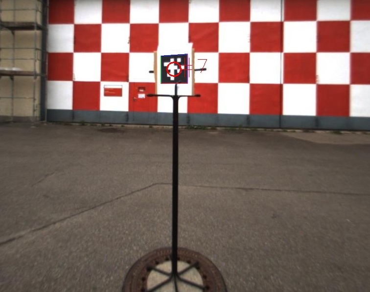
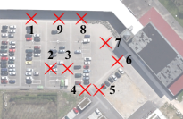
Figure 5: The left figure shows an example of an AprilTag placed above a manhole from where a panoramic image was acquired. The right figure illustrates an aerial view of the parking lot for the parking lot experiment. Red crosses highlighting the positions of the panoramas. The numbers represent the AprilTag ID.

IV-A Metric Accuracy Quantification

The parking lot experiment is designed to evaluate the accuracy of our method. It is full of dynamic objects and visual aliasing. Additionally, most of the structures and buildings are only on the far-away perimeter of the parking lot.

Using GPS as ground truth is not sufficient as our method aims at providing accurate estimations, potentially better than GPS accuracy. For reference, we collected spherical panoramas by using a smartphone, on visually distinct landmarks such as manholes. Then, as a ground truth we placed visual fiducials, namely AprilTags [20] above the manholes from where the panoramas were acquired. The fiducials serve as a way to compute the ground truth positions of the manually acquired panoramas. AprilTags come with a robust detector and allow for precise 3D positioning. We use the tag family 36h11 and the open source implementation available from  [11]. Figure 5 shows one such tag from the view of the camera with the tag detection and detected id superimposed on the image. Figure 5 also illustrates the aerial view of parking lot with the position from where the panoramas were generated (red crosses). The numbers represent IDs for each April Tag. To have a fine estimate of the panoramic image pose, we use non-linear least squares to optimize for the full 6D tags positions from the computed camera poses as illustrated in Figure 6.

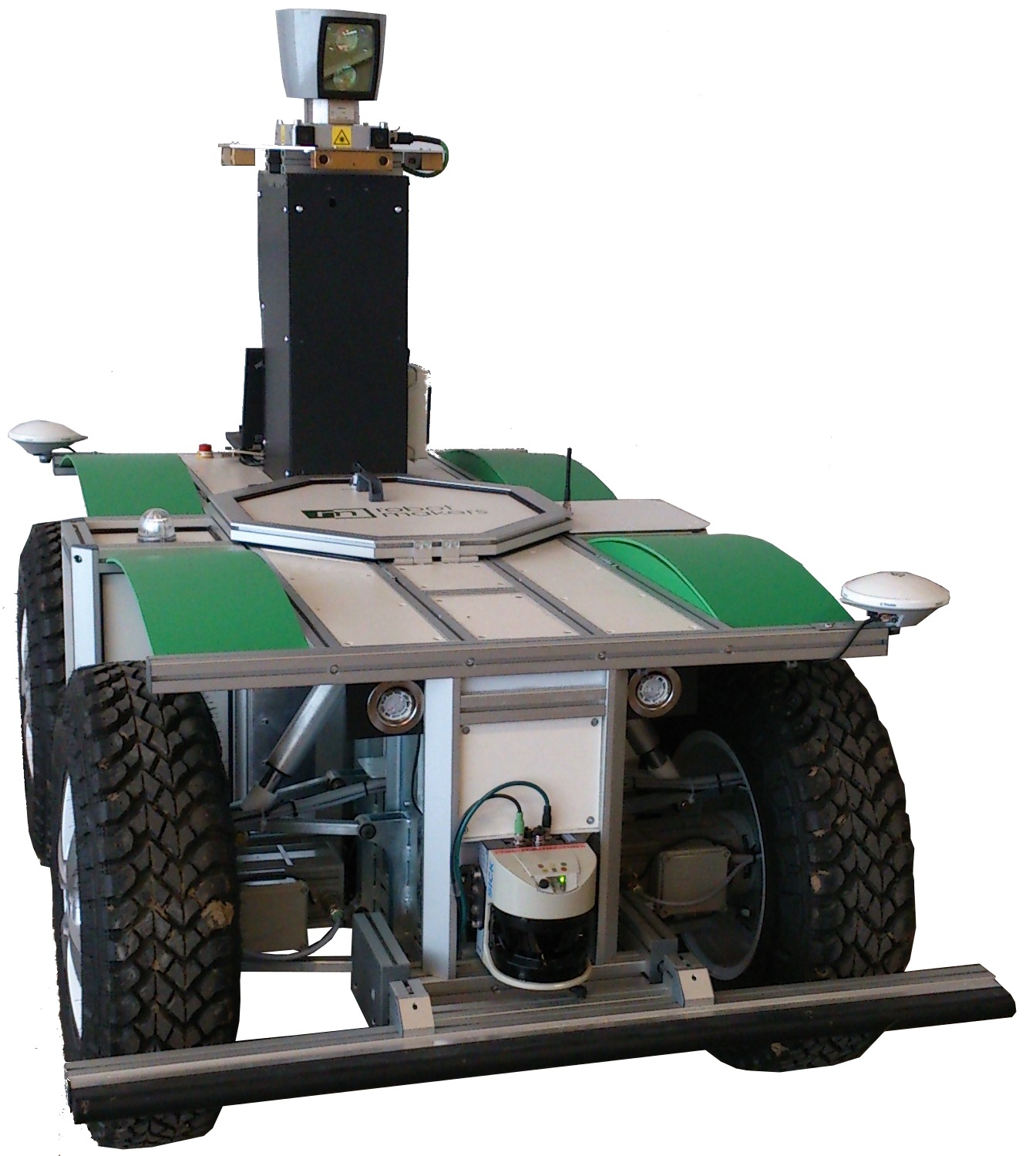
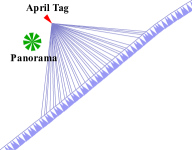
Figure 6: The left figure shows the robot used to conduct the parking lot experiments and the right figure illustrates the final monocular camera positions with the estimated position of the panorama and April tag in the parking lot.

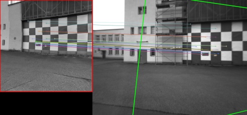
(a) $135$

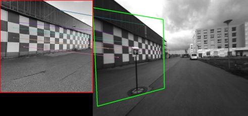
(b) $180$

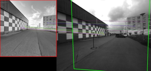
(c) $225$

Figure 7: Matching 3 views of the same panorama to monocular images. $90^{\circ}$ field-of-view rectilinear projections and the corresponding feature matches for each view can be seen. Homography projection of the panoramas on the monocular image is shown in green.

For these experiments, we used a robot equipped with an odometry estimation system and a monocular 100^∘ wide field-of-view camera. We performed $4$ runs around all $9$ AprilTags and $1$ shorter run. In total we performed a total of $5$ different runs in the parking lot. The position of panoramas and AprilTags are computed with respect to the camera positions. Tables IV-A and IV-A report the error between the computed pose of the panorama and the associated tag for the $5$ runs.  Figure 7 shows examples of feature matches between three panorama views and camera images. Each of the three images in Figure 7 show the matched features and homography of the rectified panorama projected on to the image acquired from the monocular camera.

1	2	3	4	5	6	7	8	9
6.00	3.14	0.99	1.65	5.36	2.94	1.22	0.53	1.29
0.72	1.07	-	9.62	4.91	2.00	5.53	0.70	1.28
-	-	-	-	-	3.35	0.74	1.07	4.03
-	-	0.37	1.03	3.92	5.34	2.07	0.39	1.07
-	0.47	0.58	0.37	12.38	5.89	1.53	0.55	2.59

TABLE I: Error (in meters) between estimated pose of each individual panoramic view compared to the ground truth tag.

TABLE II: Error (in meters) between estimated pose of the connected panoramic views compared to the ground truth tag.

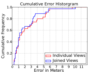
Figure 8: Cumulative error histogram for the parking lot experiment. The optimization of the connected panoramic views (blue) improves the performance.

The errors reported in Table IV-A correspond to optimizing the individual views of the panoramas without any constraints among them. This corresponds to the optimization in Eq. 13. That is, if two views of a panorama match at a certain place, we optimize them independent of each other. Table IV-A reports errors when all the views of the panoramas are connected together. This corresponds to the optimization in Eq. 14. Connecting views from the same panorama together improves the accuracy as can be seen from Figure 8. The system does not report localization results if the matching rectilinear views are estimated too far with respect to the current pose.

The panorama acquired from the position of tag id 5 and 6 is localized with least accuracy as most of the estimated 3D features are far way ($>50m$). The panoramas acquired from the position of tags 8 and 9 are localized with the highest accuracy as the tracked features are relatively closer ($15m-20m$).

As expected, the localization accuracy decreases with increase in the distance to tracked features. Points that are far away from the camera show small motion. In these cases, small errors in the odometry estimate and in the keypoint position in the image cause considerable errors in the estimated feature distances in 3D. Nevertheless, about 40% of the runs we are within a $1m$ accuracy, 60 % within $1.5m$. This is significantly lower than the accuracy on mobile devices (5 to 8.5 m) which use cellular network and GPS [28].

Despite our efforts in providing accurate ground truth, this is not free of errors. Especially because the exact center of the panorama is unknown. Manually acquired panoramas are difficult to generate and often the camera center moves. The individual images which are stitched together often do not share the same exact camera center.

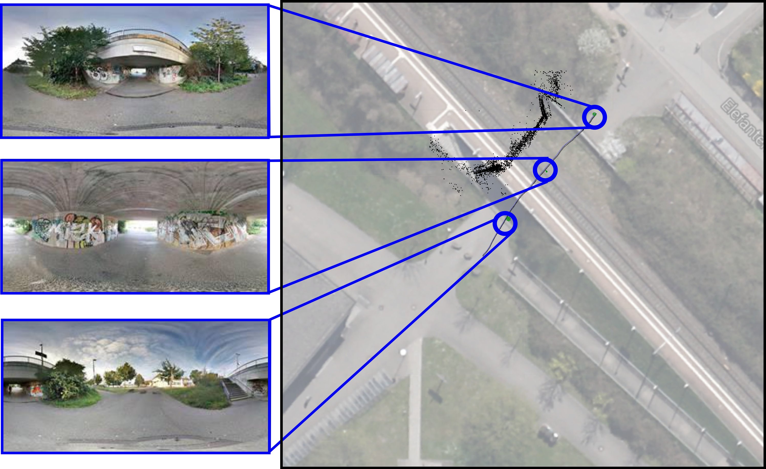
Figure 9: Matches between monocular images and Street View panoramas for a railway underpass used for the Tango experiments. The middle image shows the aerial imagery of the location, superimposed with localization results of the panoramic view with respect to the camera trajectory. The second panorama is acquired under the bridge while the other two are outside. The images on the right show example matches that were found between the monocular images and extracted rectilinear panoramic views.

IV-B Urban Localization with a Google Tango Device

In order to show the flexibility of our approach, we evaluated our algorithm with a Google Tango device in two urban environments. We used the integrated visual inertial odometry estimated on the Tango device for our method. Tango has two cameras: one that has a high resolution but a narrow field-of-view, and another one, that has a lower resolution but a wider field-of-view. The narrow field-of-view camera has a frame rate of $5$Hz, the other streams at $30$Hz. We use the higher resolution camera as the monocular image source for our framework, meanwhile the wide angle camera is used internally by the device for the odometry estimates. Throughout our experiments, we found the odometry from Tango to be significantly more accurate indoor than outdoor. This is probably due to a relatively weak feature stability outdoors and the presence of only small baselines when navigating in wide areas. To alleviate this problem, we mounted a mirrored $45-90-45$ prism on the narrow-field-of-view camera and pointed the wide field-of-view to the floor. In this way, the Tango device reliably tracks features on the asphalt and computes accurate odometry estimates, meanwhile the other camera points at the side. Figure 11 shows the prism mounted Tango device.

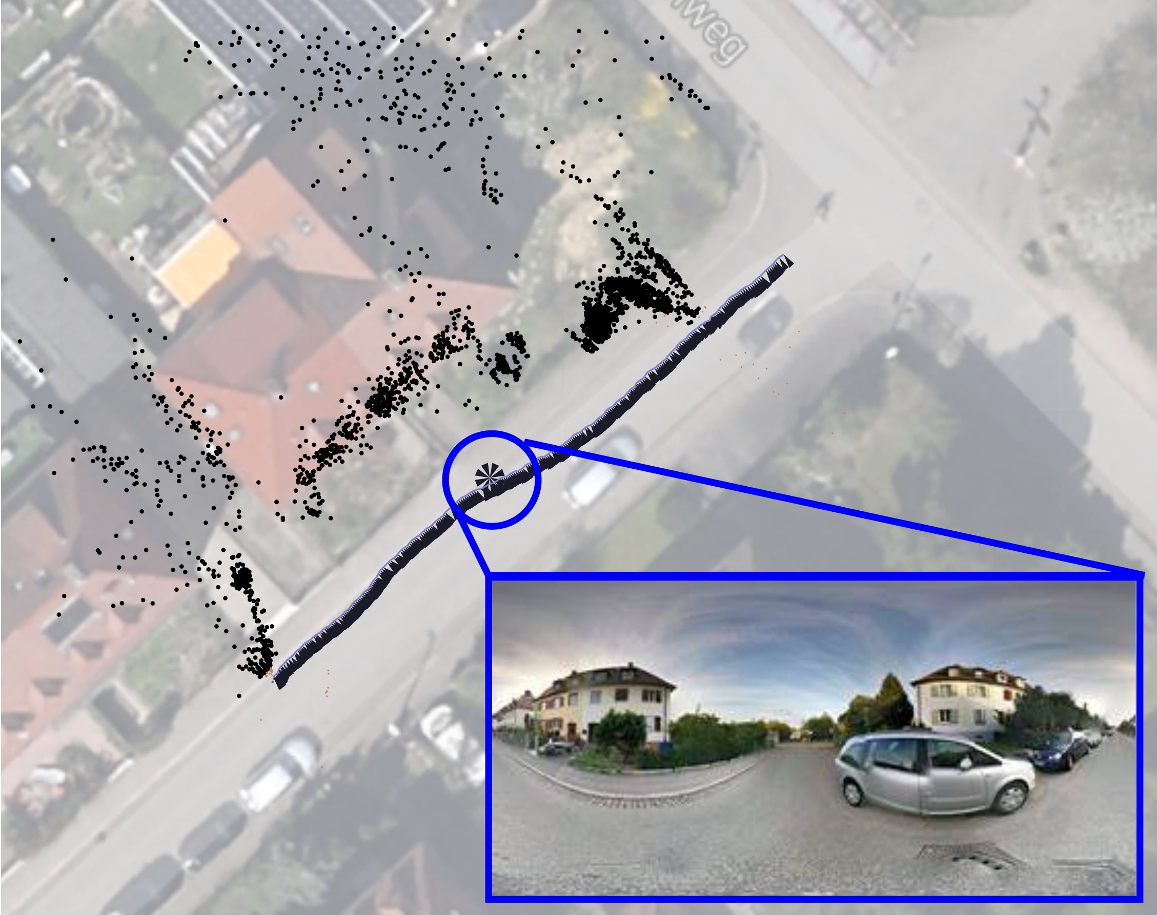
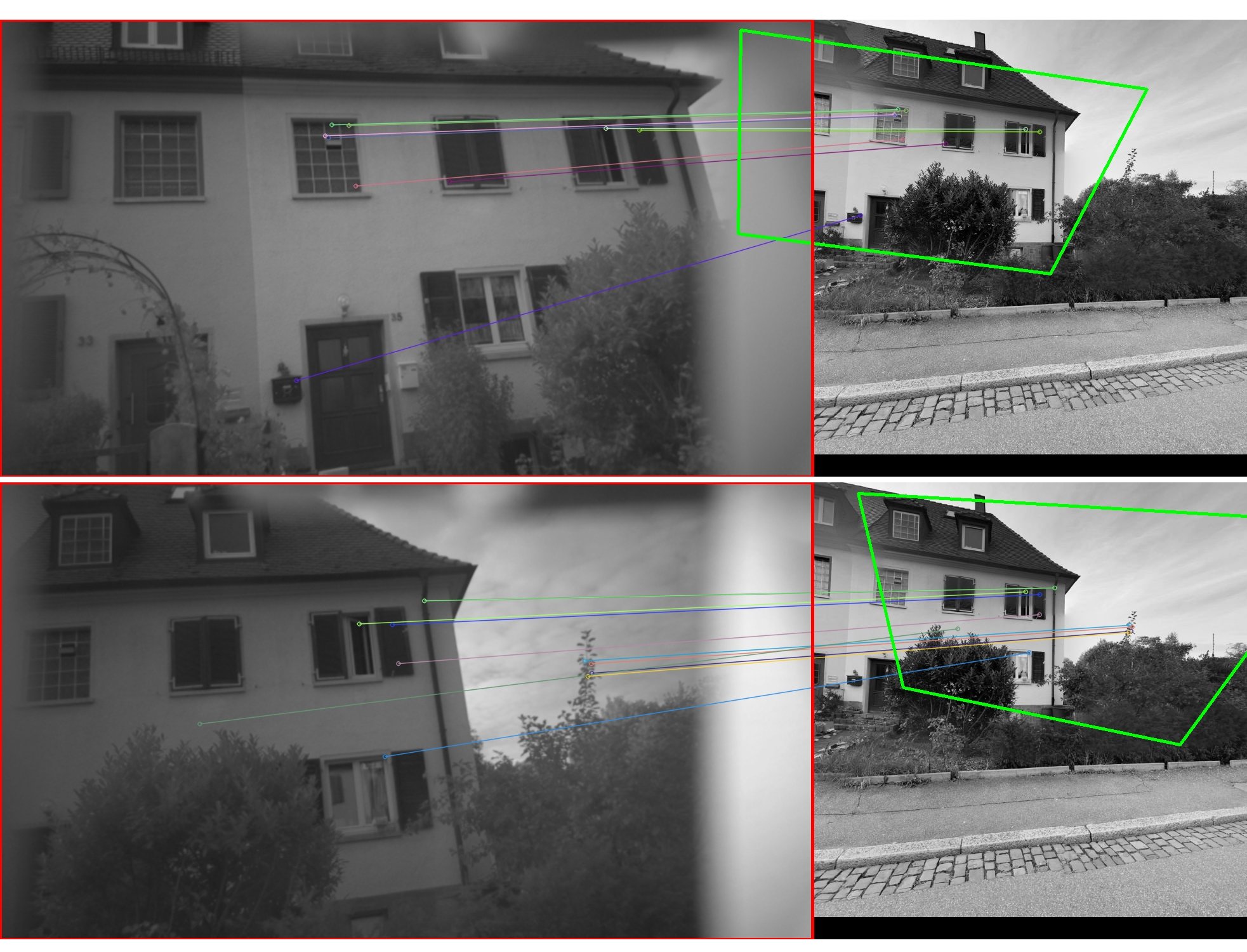
Figure 10: Optimized 3D points with the estimated panorama position overlayed on Google maps (top). An example of matching between panorama views and Google Tango images. As both cameras are pointing in different directions, the features used internally for visual inertial odometry are different from the features used for localizing Street View panoramas.

The first urban scenario has been run on roads around the University campus in Freiburg, Germany. In particular, around the area with GPS coordinates $48.0125518,7.8322567$. The panoramas used in the Tango experiments are public and can be viewed on Street View. In the experiment, we crossed a railway line by using an underpass where GPS connection is lost, see Figure 9. Our method is able to estimate 3D points from the images acquired from Tango and then match them to the nearby panoramic images, see Figure 9. Then, we moved into the suburban road with houses on both sides. This location is challenging due to the fact that all houses look similar. Also in this case, our approach is able to correctly estimate the 3D points of the track and localize the nearest panorama, see Figure 10. In the figure, the black points are the estimated 3D points while the circles in the center of the image are the positions of the panorama views. The pose of the Tango device is overlayed on the street.

To test our technique in a Street View panorama acquired by Google, we ran another experiment on the main road of the village of Marckolsheim, France. Despite being a busy road, our technique correctly estimated 3D points from the Tango image stream and successfully estimated the panorama positions, see Figure 1.

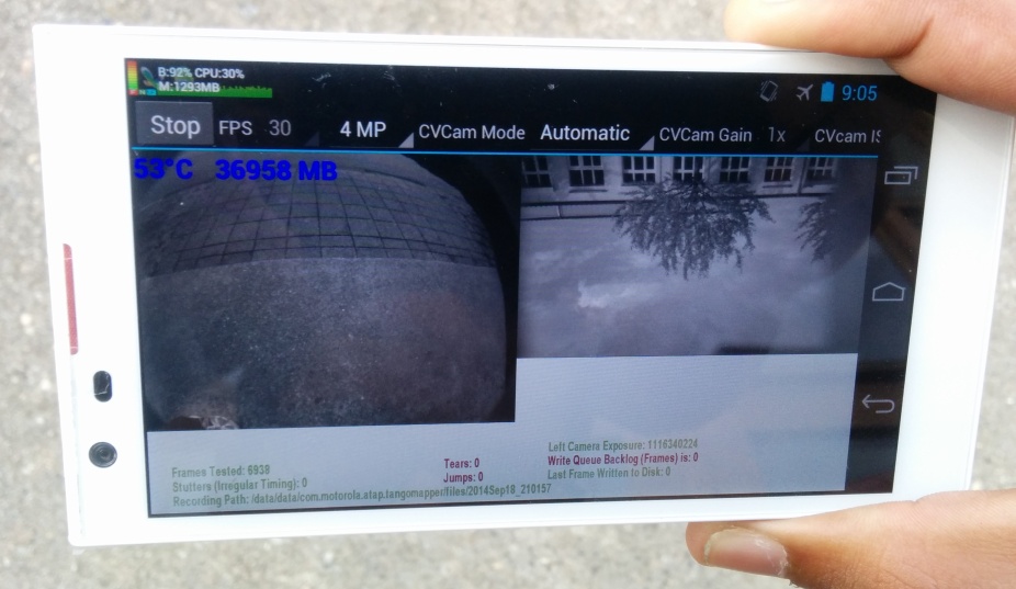
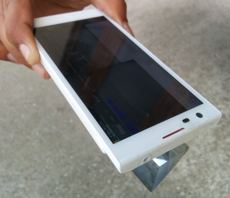
Figure 11: Google Tango with the prism attached to the narrow field of view camera. The screen shows the camera used for visual odometry pointing downwards, while the narrow field of view camera points sidewards.

V Discussion

Our method can use any kind of odometric input. In the case of Tango, the odometry is based on the work of Mourikis and Roumeliotis [18] that makes use of visual odometry and IMUs to generate accurate visual-inertial odometry (VIO). This system is offered by the Google’s Tango device libraries. When implemented on Tango, our method uses the two onboard cameras. One is the wide angle camera, that is used exclusively for VIO and the other is the narrow FOV camera, that is used for matching against Street View imagery. It is important to note that they point in different directions and do not share views. For this reason, the resulting features for VIO and 3D localization are not directly correlated. Note also that our two step optimization can in principle be done in one step. Our choice to do it in two steps resulted from a practical perspective: the first is used to compute a good initial solution for the second optimization. For the scope of this paper, we are not interested in using the panoramas to build an accurate large model of the environment: we aim at localizing without building new large scale maps where Street View exists.

VI Conclusion

In this paper, we present a novel approach to metric localization by matching Google’s Street View imagery to a moving monocular camera. Our method is able to metrically localize without requiring a robot to pre-visit locations to build a map where Street View exists.

We model the problem of localizing a robot with Street View imagery as a non-linear least squares estimation in two phases. The first estimates the 3D position of tracked feature points from short monocular camera streams, while the second computes the rigid body transformation between the points and the panoramic image. The sensor requirements of our technique are a monocular image stream and odometry estimates. This makes the algorithm easy to deploy and affordable to use. In our experiments, we evaluated the metric accuracy of our technique by using fiducial markers in a wide outdoor area. The results demonstrate high accuracy in different environments. Additionally, to show the flexibility and the potential application of this work to personal localization, we also ran experiments using images acquired with Google Tango smartphone in two different urban scenarios. We believe that this technique paves the way towards a new cheap and widely useable outdoor localization approach.

References

- Agarwal et al. [2014] P. Agarwal, G. Grisetti, G. D. Tipaldi, L. Spinello, W. Burgard, and C. Stachniss. Experimental analysis of dynamic covariance scaling for robust map optimization under bad initial estimates. In Proceedings of the IEEE International Conference on Robotics and Automation (ICRA), 2014.
- Agrawal and Konolige [2008] M. Agrawal and K. Konolige. FrameSLAM: From Bundle Adjustment to Real-Time Visual Mapping. IEEE Transactions on Robotics, 24(5):1066–1077, 2008.
- Anguelov et al. [2010] D. Anguelov, C. Dulong, D. Filip, C. Frueh, S. Lafon, R. Lyon, A. Ogale, L. Vincent, and J. Weaver. Google street view: Capturing the world at street level. Computer, (6):32–38, 2010.
- Cummins and Newman [2009] M. Cummins and P. Newman. Highly scalable appearance-only SLAM - FAB-MAP 2.0. In Proceedings of Robotics: Science and Systems (RSS), 2009.
- Davison et al. [2007] A. J. Davison, I. D. Reid, N. D. Molton, and O. Stasse. Monoslam: Real-time single camera slam. IEEE Transactions on Pattern Analysis and Machine Intelligence (PAMI), 29(6):1052–1067, 2007.
- Dellaert [2005] F. Dellaert. Square root SAM. In Proceedings of Robotics: Science and Systems (RSS), pages 177–184, 2005.
- Fei-Fei and Perona [2005] L. Fei-Fei and P. Perona. A bayesian hierarchical model for learning natural scene categories. In Proceedings of the IEEE Computer Society Conference on Computer Vision and Pattern Recognition (CVPR), volume 2, pages 524–531. IEEE, 2005.
- Fuentes-Pacheco et al. [2012] J. Fuentes-Pacheco, J. Ruiz-Ascencio, and J. M. Rendón-Mancha. Visual simultaneous localization and mapping: a survey. Artificial Intelligence Review, pages 1–27, 2012.
- Google Inc. [2012] Google Inc. The never-ending quest for the perfect map. http://googleblog.blogspot.de/2012/06/never-ending-quest-for-perfect-map.html/, 2012.
- Irschara et al. [2009] A. Irschara, C. Zach, J.-M. Frahm, and H. Bischof. From structure-from-motion point clouds to fast location recognition. In Proceedings of the IEEE Computer Society Conference on Computer Vision and Pattern Recognition (CVPR), pages 2599–2606, 2009.
- Kaess [2013] M. Kaess. AprilTags C++ Library, 2013. URL http://people.csail.mit.edu/kaess/apriltags.
- Kaess et al. [2012] M. Kaess, H. Johannsson, R. Roberts, V. . Ila, J. J. Leonard, and F. Dellaert. iSAM2: Incremental smoothing and mapping using the Bayes tree. International Journal of Robotics Research (IJRR), 31(2):216–235, 2012.
- Klingner et al. [2013] B. Klingner, D. Martin, and J. Roseborough. Street view motion-from-structure-from-motion. In IEEE International Conference on Computer Vision (ICCV), pages 953–960, 2013.
- Kümmerle et al. [2011] R. Kümmerle, G. Grisetti, H. Strasdat, K. Konolige, and W. Burgard. g2o: A general framework for graph optimization. In Proceedings of the IEEE International Conference on Robotics and Automation (ICRA), pages 3607–3613, 2011.
- Lowe [2004] D. G. Lowe. Distinctive image features from scale-invariant keypoints. International Journal of Computer Vision, 60(2), 2004.
- Majdik et al. [2013] A. L. Majdik, Y. Albers-Schoenberg, and D. Scaramuzza. MAV urban localization from Google street view data. In Proceedings of the IEEE/RSJ International Conference on Intelligent Robots and Systems (IROS), pages 3979–3986, 2013.
- Majdik et al. [2014] A. L. Majdik, D. Verda, Y. Albers-Schoenberg, and D. Scaramuzza. Micro air vehicle localization and position tracking from textured 3d cadastral models. In Proceedings of the IEEE International Conference on Robotics and Automation (ICRA), pages 920–927, 2014.
- Mourikis and Roumeliotis [2007] A. I. Mourikis and S. I. Roumeliotis. A multi-state constraint kalman filter for vision-aided inertial navigation. In Proceedings of the IEEE International Conference on Robotics and Automation (ICRA), pages 3565–3572, 2007.
- Muja and Lowe [2012] M. Muja and D. G. Lowe. Fast matching of binary features. In Computer and Robot Vision (CRV), pages 404–410, 2012.
- Olson [2011] E. Olson. AprilTag: A robust and flexible visual fiducial system. In Proceedings of the IEEE International Conference on Robotics and Automation (ICRA), 2011.
- Sattler et al. [2012a] T. Sattler, B. Leibe, and L. Kobbelt. Improving image-based localization by active correspondence search. In Proceedings of the European Conference on Computer Vision (ECCV), pages 752–765, 2012a.
- Sattler et al. [2012b] T. Sattler, T. Weyand, B. Leibe, and L. Kobbelt. Image retrieval for image-based localization revisited. In British Machine Vision Conference (BMVC), page 7, 2012b.
- Thrun [2002] S. Thrun. Robotic mapping: A survey. In G. Lakemeyer and B. Nebel, editors, Exploring Artificial Intelligence in the New Millenium. Morgan Kaufmann, 2002.
- Torii et al. [2009] A. Torii, M. Havlena, and T. Pajdla. From google street view to 3d city models. In Computer Vision Workshops (ICCV Workshops), 2009.
- Torii et al. [2011] A. Torii, J. Sivic, and T. Pajdla. Visual localization by linear combination of image descriptors. In Computer Vision Workshops (ICCV Workshops), 2011.
- Triggs et al. [2000] B. Triggs, P. F. McLauchlan, R. I. Hartley, and A. W. Fitzgibbon. Bundle adjustment—a modern synthesis. In Vision algorithms: theory and practice, pages 298–372. Springer, 2000.
- Zamir and Shah [2010] A. R. Zamir and M. Shah. Accurate image localization based on google maps street view. In Proceedings of the European Conference on Computer Vision (ECCV), pages 255–268, 2010.
- Zandbergen and Barbeau [2011] P. A. Zandbergen and S. J. Barbeau. Positional accuracy of assisted gps data from high-sensitivity gps-enabled mobile phones. Journal of Navigation, 64(03):381–399, 2011.
- Zhang and Kosecka [2006] W. Zhang and J. Kosecka. Image based localization in urban environments. In 3D Data Processing, Visualization, and Transmission, Third International Symposium on, pages 33–40. IEEE, 2006.