Equilibria of point charges on convex curves

Abstract.

We study the equilibrium positions of three points on a convex curve under influence of the Coulomb potential. We identify these positions as orthotripods, three points on the curve having concurrent normals. This relates the equilibrium positions to the caustic (evolute) of the curve. The concurrent normals can only meet in the core of the caustic, which is contained in the interior of the caustic. Moreover, we give a geometric condition for three points in equilibrium with positive charges only. For the ellipse we show that the space of orthotripods is homeomorphic to a 2-dimensional bounded cylinder.

1. Introduction

The electrostatic (Coulomb) potential of a system of point charges confined to a certain domain in Euclidean plane has been studied in a number of papers in connection with various problems and models of mathematical physics [2], [7], [12]. Analogous problems for the gravitational potential of point masses have also been discussed in the literature [2], [7], [12].

Several issues considered in the mentioned papers were connected with studying equilibria configurations of a system of point charges. As usual, a configuration $P$ of several points on a curve $X$ is called an equilibrium for a system of charges $Q$ if the system is ‘at rest’ at this configuration. In particular, equilibria of three point charges on an ellipse have been discussed in some detail in [2].

In this paper, we deal with a specific problem related to our previous research of charged polygonal linkages [10]. Namely, given a collection of $n\geq 3$ points $P$ on a given (fixed) closed curve $X$, we wish to investigate if this collection of points is an equilibrium of $E_{q}$ for a certain system of point charges $q$. If this is possible, any such collection of charges $q$ will be called balancing charges for $P$. We also want to investigate if this can be done with positive charges only. An analogous definition is meaningful and interesting for several other potentials of point interactions, e.g., for gravitational potential or logarithmic potential in the plane and more general central forces.

In the sequel we deal mostly with the (electrostatic) Coulomb potential $E_{q}$ and the $E_{q}$-equilibrium problem for triples of points on a closed curve in the plane. We reveal that this problem is closely related to certain geometric issues concerned with the concept of caustic (evolute) of a plane curve and present several results along these lines. In particular, we give a geometric criterion for balancing three points on an arbitrary closed curve (Theorem 1) and present a condition for balancing with positive charges (Proposition 2). We give a description of the set of triples which can be balanced on an ellipse, and also a description of the set of triples on an ellipse which can be balanced by positive charges. Some related results and arising research perspectives are discussed in the last section of the paper.

An important observation is that Coulomb forces can be replaced by Hooke forces produced by (either compressed or extended) connecting springs, or by any other central forces.

2. Electrostatic equilibrium of points on closed curve

2.1. Condition for triples in equilibrium

We consider a collection $P_{1},\cdots,P_{n}$ of distinct points on a smooth curve $X$ in the plane, together with charges $q_{1},\cdots,q_{n}$. We do not require in this section that the curve is convex. The Coulomb potential of these point charges is given by

$$E_{q}=-\sum_{i<j}\frac{q_{i}q_{j}}{d_{ij}},$$

where $p_{i}=\overrightarrow{OP_{i}}$, and $d_{ij}=||p_{i}-p_{j}||.$ The Coulomb forces between these points are given by

$$F_{ji}=\frac{q_{i}q_{j}}{d_{ij}^{3}}(p_{i}-p_{j})$$

Let $F_{i}=\sum_{j\neq i}F_{ji}$ be the resultant of these forces at $P_{i}$. Let $T_{i}$ be the tangent vector to the curve $X$ at the point $P_{i}$.

Definition 1.

A collection of points on a curve $X$ charged by $q=(q_{1},\cdots,q_{n})\neq(0,...,0)$ is called an $E_{q}$-equilibrium (or is $E_{q}$-balanced) if, at every point $P_{i}$ of the collection, the resultant of the forces is orthogonal to $T_{i}$:

$$\langle F_{i},T_{i}\rangle=\sum_{j\neq i}\frac{q_{i}q_{j}}{d_{ij}^{3}}\langle p_{i}-p_{j},T_{i}\rangle=0\;\;\forall i.$$

In this situation we say that the charges $q$ are balancing for $P_{1},\cdots,P_{n}$.

Notice that $E_{q}$-equilibria correspond to the critical/stationary points of the potential $E_{q}$.

Whenever $q_{i}=0$ for one of the charges, the system reduces to a system with one point less (the removed point can be on an arbitrary place). If none of the charges is zero then the equilibrium condition implies a system of linear equations for the values of balancing charges.

In the special case of two points we have two equations. Non-zero solutions $q=(q_{1},q_{2})$ only occur if $P_{1}P_{2}$ is orthogonal to both $T_{1}$ and $T_{2}$. So $P_{1}P_{2}$ is a double normal of the curve.

The main situation of our study is three points on a curve. In this case we have the matrix equation:

$$\begin{pmatrix}0&a_{12}&a_{13}\\ a_{21}&0&a_{23}\\ a_{31}&a_{32}&0\end{pmatrix}\begin{pmatrix}q_{1}\\ q_{2}\\ q_{3}\end{pmatrix}=0\;,\;\mbox{where}\;\;a_{ij}=\frac{\langle p_{i}-p_{j},T_{i}\rangle}{d_{ij}^{3}}\;.$$

If the rank of this system is 3 then its solution is only the triple $(0,0,0)$ so a genuine (non-trivial) equilibrium is impossible. Thus non-trivial stationary charges may only exist if the rank of this system does not exceed two.

Definition 2.

Points $P_{1},P_{2},P_{3}$ satisfy the corank 1 condition if the rank of the matrix

$$(a_{ij})=\Big{(}\frac{\langle p_{i}-p_{j},T_{i}\rangle}{d_{ij}^{3}}\Big{)}$$

is less than or equal to $2$.

If the rank of the matrix $(a_{ij})$ is equal to 2, then the matrix equation has a one-dimensional solution space and therefore defines a unique point $[q_{1}:q_{2}:q_{3}]$ in $\mathbb{P}^{2}$. In case where the rank of this matrix is 1 it follows that the points $P_{1},P_{2},P_{3}$ are collinear and at least one of $P_{i}P_{j}$ is a double normal. This case cannot occur if the curve is convex.

Proposition 1.

Points $P_{1},P_{2},P_{3}$ satisfy the corank 1 condition if and only if the three normals at these points are concurrent, that is, have a common point.

Proof.

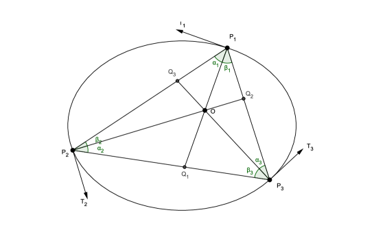
Figure 1. Orthotripods and Ceva configuration

Introducing the angles $\alpha_{i}=\angle{P_{i+1},P_{i}Q_{i}}$, $\beta_{i}=\angle{Q_{i}P_{i}P_{i-1}}$ (with mod 3 convention) and unit tangent vectors $T_{i}$, we notice that

$$a_{12}=\frac{\langle p_{1}-p_{2},T_{1}\rangle}{d_{12}^{3}}=-\frac{\sin\alpha_{1}}{d_{12}^{2}},\;\;\;\;\;\;a_{13}=\frac{\langle p_{1}-p_{3},T_{1}\rangle}{d_{13}^{3}}=\frac{\sin\beta_{1}}{d_{13}^{2}},\;\;\;\mbox{etc.}$$

We conclude that $\operatorname{rank}(a_{ij})$ does not exceed two if and only if

$$a_{12}a_{23}a_{31}+a_{13}a_{21}a_{32}=0.$$

The latter condition is equivalent to

$$\sin\alpha_{1}\sin\alpha_{2}\sin\alpha_{3}=\sin\beta_{1}\sin\beta_{2}\sin\beta_{3}.$$

By Ceva theorem the lines $P_{1}Q_{1},P_{2},Q_{2},P_{3}Q_{3}$ are concurrent if and only if the signed lengths of segments satisfy the following relation.

$$\frac{P_{2}Q_{1}}{Q_{1}P_{3}}\cdot\frac{P_{3}Q_{2}}{Q_{2}P_{1}}\cdot\frac{P_{1}Q_{3}}{Q_{3}P_{2}}=1,$$

which is in our case equivalent to

$$\frac{\sin\alpha_{1}}{\sin\beta_{1}}\cdot\frac{\sin\alpha_{2}}{\sin\beta_{2}}\cdot\frac{\sin\alpha_{3}}{\sin\beta_{3}}=1.$$

∎

Remark. The same proposition holds for any central forces, that is, for all the forces that are given by:

$$F_{ji}=\frac{q_{i}q_{j}}{f_{ij}}(p_{i}-p_{j})\;\;\mbox{where}\;\;f_{ij}=f_{ji}\;\mbox{depends only on}\;\;d_{ij}.$$

Examples of central forces are Coulomb forces, Hooke forces, and logarithmic forces. The Ceva equation does not depend on the concrete central force, since the denominators of $a_{ij}$ cancel in the condition of Proposition 1. We can as well work with $a_{ij}=\langle p_{i}-p_{j},T_{i}\rangle$. Proposition 2 below also holds in this more general case.

Remark. The claim of Proposition 1 involves only the points $P_{i}$ and the tangent vectors $T_{i}$ and no other data of the curve.

Definition 3.

An orthotripod on a smooth closed curve $X$ is defined as an unordered triple of distinct points such that the normals to $X$ at these points are concurrent. The common point of these three normals is called the orthotricentre.

Notice an analogy of this result with a well-known description of three forces in equilibrium.

Remark. The name ”tripod” was used by S. Tabachnikov in [13] for three concurrent normals to the curve making angles of 120 degrees (Steiner property).
Orthotripods occur also in [3] and [11], where the authors give a necessary condition for immobilization of convex curves by three points. In those papers they are called normal triples.

Theorem 1.

Given 3 points on a curve $X$, there exist charges $(q_{1}:q_{2}:q_{3})$ such the points are in $E_{q}$-equilibrium if and only if they form an orthotripod on $X$.

Proof.

Follows from Proposition 1. ∎

In such a case the values of balancing charges can be explicitly calculated (cf. Section 4). For the moment we search for positive balancing charges.

Proposition 2.

If $P_{1},P_{2},P_{3}$ satisfy the corank 1 condition, then there exist positive balancing charges if and only if the three normals at points $P_{i}$ enter the interior of triangle $\triangle P_{1}P_{2}P_{3}$.

Proof.

For a solution $(q_{1},q_{2},q_{3})$ with all $q_{i}>0$, we have

$\mbox{sign}\;a_{12}=-\mbox{sign}\;a_{13}$

$\mbox{sign}\;a_{21}=-\mbox{sign}\;a_{23}$

$\mbox{sign}\;a_{31}=-\mbox{sign}\;a_{32}$.

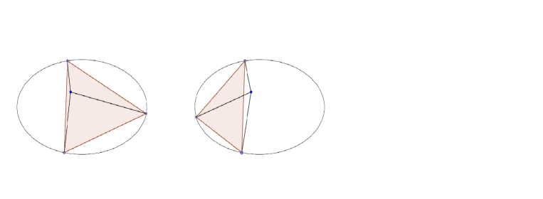
Figure 2. Orthotripods in equilibrium, with positive charges (left) and different signs (right)

Since (up to a positive factor) $a_{12}=\langle p_{1}-p_{2},T_{1}\rangle$ and $a_{13}=\langle p_{1}-p_{3},T_{1}\rangle$ it follows that the edges $P_{1}P_{2}$ and $P_{1}P_{3}$ are on different sides of the normal at $P_{1}$ . ∎

3. Caustics

The above results indicate an interesting connection with some classical issues of differential geometry which we outline below. To this end we will need some definitions and auxiliary results to be used in the sequel.

Definition 4.

Caustic $C(X)$ of a regular closed curve $X$ is defined as the set of curvature centers at all points of $X$ (also known as evolute or focal set).

It is known that caustic may be equivalently defined as the envelope of normals to $X$ or the set of singular points of the wavefront of parallel curves (on a given distance of $X$) [4]. For a generic curve $X$, its caustic is a piecewise smooth curve with cusps and normal crossings as singularities (see, e.g. [1]). Notice also that all parallel curves have the same caustic as $X$. They share with $X$ all properties, which can extracted from the caustic.

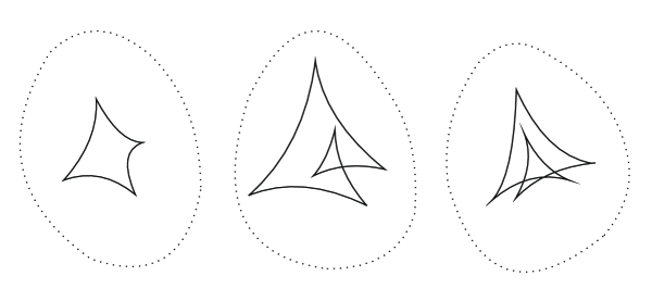
Figure 3. Some curves and their caustics

Our next aim is to describe in some detail the relation between caustics and orthotripods. In order to explore further aspects of this connection we need some more definitions and notation. We assume that the curve $X$ is parameterized by its arclength and write $X(s)$. Denote by $T(s)$ the unit tangent vector and by $N(s)$ the unit normal vector such that the pair $T(s),N(s)$ is positively oriented. Let the function $D:{\mathbb{R}}^{2}\times X\rightarrow{\mathbb{R}}$ be given by

$$D(x,y,s)=|(x,y)-X(s)|^{2}.$$

The critical set $M=\{(x,y,s):\partial_{x}D=\partial_{y}D=0\}$ of the mapping $D$ is generically smooth and the projection $\Pi:M\rightarrow{\mathbb{R}}^{2}$ is a mapping between smooth two-dimensional manifolds. The image of the critical set $M$ is exactly the caustic $C(X)$ defined above.

For a point $Q\in{\mathbb{R}}^{2}$, a pair $(Q,P)$ belongs to the preimage $\Pi^{-1}(Q)$ iff the normal to the curve $X$ through $P$ contains $Q$. Thus the number of points in the preimage of $Q$ is equal to the number of normals to the curve $X$ emerging from $Q$. This number is even if $Q$ does not belong to caustic. Notice that if we count the preimages with signs then we get the degree of $\Pi$ which vanishes.

For further use we mention a few other properties of $\Pi$. In particular, the map $\Pi$ at a singular point $(Q,P)$ is a fold map if $\kappa^{\prime}(P)\neq 0$, and it is a cusp map if $\kappa^{\prime}(P)=0$ and $\kappa^{\prime}(P)$ has a simple zero at $P$, where $\kappa(P)$ is the curvature at the point $P$.

In the rest of this section we assume that $X$ is a convex curve and that $\kappa(P)\neq 0$ (no flat points). Then the caustic $C(X)$ divides the plane in closed domains. For each of the points $Q$ of the plane let us denote by $n(Q)$ the number of normals to the curve $X$ emerging from $Q$. This number is constant on each of the (interiors of the) domains. Points from the non-compact domain have only (exactly) two normals to $X$.

Definition 5.

The union of the compact domains is called the interior region of the caustic. The core of the caustic is defined as the union of the closed domains where the points have at least four emerging normals.

The co-orientation of the caustic along the fold-lines (in the direction of two extra normals) together with the orientation of the plane ${\mathbb{R}}^{2}$ yield an orientation of the caustic. Let for any point $Q$ in the complement of the caustic $i(Q)$ be the degree of $Q$ with respect to the caustic.

Lemma 1.

In the above notation, we have:

1. $n(Q)=2i(Q)+2$.

2. The core of the caustic is equal to the closure of the set of points $Q$ with $i(Q)\neq 0$.

Proof.

The index of point with respect to a closed curve can be computed by taking a generic half-ray starting at that point and counting the intersection points with the curve with a sign. Outside a compact area $i(Q)=0$, while $n(Q)=2$. For each intersection point of the ray with the caustic, the number of normals changes by $+2$ (respectively, $-2$) according to the change $+1$ (respectively, $-1$) of the index. ∎

From the above discussion and Lemma 1 we get a characterization of the set of orthotricenters.

Proposition 3.

The set of orthotricenters is a compact subset of the interior region of the caustic and coincides with the core of the caustic.

Remark. In the paper of Gounai and Umehara [8] is shown that there are exactly 3 types of caustics with 4 cusps only (Figure 4). Inspection of these cases shows that the core can be different from the internal region. Lemma 1 implies that there are only 2 normals in the ”holes”.

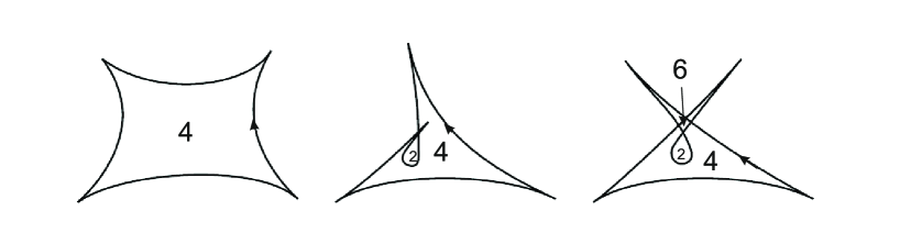
Figure 4. The three 4-vertex caustics with orientation and the values $n(Q)$.

Hence for studying orthotripods we only need to consider orthotricenters in the core of caustic.

Next we discuss the equilibria with positive charges. Double normals to $X$ provide an extra structure. It is known that each curve has at least two double normals. There exist curves with infinitely many double normals (circle other curves of constant width) but they are highly non-generic, so here we assume that the number of double normals is finite.

Lemma 2.

Assume that an orthotripod changes continuously so that the orthotricenter crosses none of double normals. Then the signs of the balancing charges do not change.

Proof.

Away from double normals, balancing charges depend continuously on the orthotripod. If one of the charges changes the sign, then by Proposition 2 the orthotricenter crosses a double normal. ∎

Double normals yield a further partition of the core of the caustic into smaller (open) regions. In each of the regions the three charges form a non-zero triple with constant signs.

4. Computing balancing charges

4.1. Balancing charges

In case the points $P_{1},P_{2},P_{3}$ satisfy the corank 1 condition (i.e. their normals form an orthotripod) we can search for the balancing charges $(q_{1},q_{2},q_{3})$. If the rank is exactly two they will define a one-dimensional subspace of ${\mathbb{R}}^{3}$. Since only the ratio is important, we have a point in ${\mathbb{P}}^{2}$. Straightforward computations show that a solution is given by:

$$[q_{1}:q_{2}:q_{3}]=[-\frac{a_{23}}{a_{21}}:-\frac{a_{13}}{a_{12}}:1]$$

We use the following notations:

$$A_{1}=\frac{a_{13}}{a_{12}}=-\;\frac{d_{12}^{2}}{d_{13}^{2}}\frac{\sin\beta_{1}}{\sin\alpha_{1}}\;,\;A_{2}=\frac{a_{21}}{a_{23}}=-\;\frac{d_{23}^{2}}{d_{12}^{2}}\frac{\sin\beta_{2}}{\sin\alpha_{2}}\;,\;A_{3}=\frac{a_{32}}{a_{31}}=-\;\frac{d_{13}^{2}}{d_{23}^{2}}\frac{\sin\beta_{3}}{\sin\alpha_{3}}.$$

Keeping in mind the corank 1 condition $A_{1}A_{2}A_{3}=-1$ we can write the solution in one of the following forms:

$$[q_{1}:q_{2}:q_{3}]=[A_{1}A_{3}:-A_{1}:1]=[-A_{3}:1:A_{2}A_{3}]=[1:A_{1}A_{2}:-A_{2}].$$

This formula is for Coulomb forces, in other cases there are similar formulas with different coefficients.

4.2. Three points on a line

Let $P_{1}$, $P_{2}$ and $P_{3}$ be located on a line in this order with distances $d_{12}=a$, $d_{23}=b$, then these points are in equilibrium if and only if

$$[q_{1}:q_{2}:q_{3}]=[\frac{1}{b^{2}}:-\frac{1}{(a+b)^{2}}:\frac{1}{a^{2}}],$$

that is, every 3 points can be balanced, but never with positive charges.

4.3. Three charges on a circle

Our original paradigm is given by the case of a circle, considered, e.g., in [6]. The following can be shown by direct calculations or as corollaries of Theorem 1 and Proposition 2.

1. Any 3 points on a circle can be balanced.

2. Three points on a circle can be balanced with positive charges iff they form an acute triangle.

4.4. Three charges on a parabola, near to the vertex

We use a parabola $y=cx^{2}$ and points $P_{1}=(-t,ct^{2}),P_{2}=(0,0),P_{3}=(t,ct^{2})$. Direct calculations shows that these points are in equilibrium iff

$$[q_{1}:q_{2}:q_{3}]=[1:-\frac{1}{4}\frac{(1+2c^{2}t^{2})^{\frac{3}{2}}}{1+c^{2}t^{2}}:1].$$

Notice that if $t\rightarrow 0$ we get $[1:-\frac{1}{4};1]$, which is in accordance with with 3 points on the line. In fact near to the vertex (on any curve) we cannot have an equilibrium with only positive charges.

4.5. Three charges on an ellipse

Several results in this case have been obtained in [2]. However some formulations in [2] are not completely rigorous and one of the aims of our research was to clarify several issues discussed in [2] in full generality. Due to our Theorem 1 and Propositions 2 and 3 we obtain mathematically rigorous statements in the case of three points on the ellipse:

1. Equilibria exist as soon as the normals are concurrent.

2. For each point in the core of the caustic there are exactly four concurrent normals, which give rise to four orthotripods. On the caustic curve itself we have only one orthotripod.

3. In general two out of four of these orthotripods correspond to equilibria with positive charges. On the double normals one has at least one charge zero.

5. Topology of orthotripods on an ellipse

If an ellipse is a circle, then the space of orthotripods is the symmetric cube of $S^{1}$ with the fat diagonal deleted.

Assume that the ellipse is not a circle. Then it has a caustic with 4 cusps and no double points. We define $\overline{T}$ as the closure of the space of orthotripods $T$ taken in the space of all unordered triples of points on the curve (the symmetric cube of $S^{1}$). Let $Y$ be the core of the caustic. In the case of the ellipse this is a topological disc bounded by 4 intervals, meeting in 4 cusps. There is a projection

$$\overline{T}\rightarrow Y,$$

sending each orthotripod to its orthotricenter.

Over the interior points of $Y$ we have a 4-sheeted covering, and $\overline{T}$ is a patch of these 4 sheets along some of the boundary edges. The rules for that are related to the fold singularities along the edges. Their fold lines separate exactly two of the sheets.

If $Q$ is an interior point of $Y$, we just number the perpendiculars counterclockwise, and then extend the numbering to all of $Y$. Sheets are now denoted (with the numbers of the perpendiculars) by $Y_{123},Y_{234},Y_{341},Y_{412}$ (no ordering involved). Next we label the cusp and the edges of the caustic with the labels of the coinciding normals:

1. $(1,2)$ means that on that edge the normals $1$ and $2$ coincide;

2. the cusp $(1,2,3)$ has the property that the normals with labels $1,2,$ and $3$ coincide.

The gluing rule for edges is now as follows. The edge $(1,2)$ is used to glue the corresponding edges of $Y_{123}$ and $Y_{412}$. On the sheets $Y_{234},Y_{341}$ there is no identification, the edge corresponding to $(1,2)$ will survive as boundary. For the other edges we have similar behavior. Around cusp points there are 3 sheets involved and the folding changes from one pair to some other pair of sheets. See the Figures 5 and 6 for the details about the gluing.

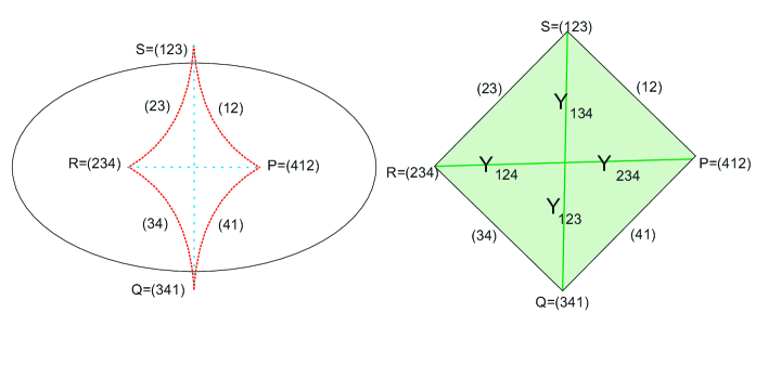
Figure 5. The ellipse and its caustic (left); Indications of regions with positive charges (right)

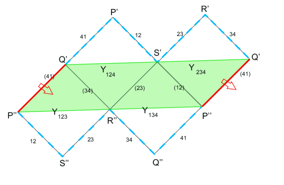
Figure 6. The cylinder of orthotripods on the ellipse. The blue dashed lines represent the boundary of the cylinder. The two thick red segments patch together. The shaded area represents the triples that can be balanced by positive charges.

We are now in a position to establish the concluding result.

Proposition 4.

Assume that we have an ellipse, which is not a circle.

1. The closure of the space of orthotripods is homeomorphic to a cylinder (with two boundary circles).

2. The space of orthotripods which can be balanced by positive charges only is homeomorphic to a cylinder.

Proof.

As we explained above, the closure of the space of orthotripods is a patch of four copies of the core of the caustic. This gives us a cylinder. On each of the copies we shade green the part that corresponds to positive charges, which gives us a smaller cylinder (see Figure 6).

∎

6. Concluding remarks and questions

As we can see from Figure 3, the combinatorics of a caustics can vary a lot. An intriguing question is to characterize the space of orthotripods in full generality, not just for ellipse (for which we have the simplest possible caustic). Evidently, similar patching rules hold for any caustic, but can lead to a more complicated topology of the space of orthotripods. Natural questions are: is this space a surface with boundary? What is its Euler characteristic? What is its genus, number of boundary components?

Another issue which remains untouched in this paper is the question of stability of an equilibrium. It seems that here more delicate characteristics of the curve are involved: not just the combinatorics of tangent lines and normals, but also the curvature of the curve.

One more interesting question could be for fixed charges $[q_{1}:q_{2}:q_{3}]$, to relate the number of orthotripods balanced by these charges to the properties of the curve.

Acknowledgements. The present paper was written during a “Research in Pairs” session in CIRM (Luminy) in January of 2015. The authors acknowledge the hospitality and excellent working conditions at CIRM

References

- [1] V.Arnol’d, A.Varchenko, S.Gusein-Zade, Singularities of differentiable maps I and II, Birkhäuser, 1985 and 1988.
- [2] J.Aguirregabiria, A.Hernandez, M.Rivas, M.Valle, On the equilibrium configuration of point charges placed on an ellipse, Computers in Physics 4, 1990, 60-63.
- [3] J.Bracho, L.Montejano, J.Urrutia, Immobilization od smooth convex figures, Geometriae Dedicata 53, 1994, 119-131.
- [4] J. W. Bruce, P. J.Giblin, Curves and Singularities, Cambridge University Press, 1992.
- [5] E.Chen, N.Lourie, Tripod configurations on curves, J. Geom. Phys. 64, 2015, 1-16.
- [6] H. Cohn, Global Equilibrium Theory of Charges on a Circle, Amer. Math. Monthly, 67, 1960, 338-343.
- [7] P. Exner, An isoperimetric problem for point iteractions, J. Phys. A: Math. Gen., A38:4795-4802, 2005.
- [8] H. Gounai, M. Umehara, Caustics of convex curves, Journal of Knot Theory and its Ramifications 23, 2014, 1-28.
- [9] L.-Y.Kao, A.Wang, The tripod configurations on curves, J. Geom. Phys. 63, 2014, 1-5.
- [10] G.Khimshiashvili, G.Panina, D.Siersma, Coulomb control of polygonal linkages, J. Dyn. Contr. Syst. 14, No.4, 2014, 491-501.
- [11] D. Mayer-Foulkes, Immobilization of smooth convex curves: Some extensions, J.Geom. 60,1997, 105-112.
- [12] J.Ross, Plotting the charge distribution of a closed-loop conducting wire using microcomputer, Amer. J. Phys. 55, 1987, 948-950.
- [13] S.Tabachnikov, The Four Vertex Theorem Revisited, Amer. Math. Monthly, 102, 1995, 912-916.