Coexistence of stable branched patterns in anisotropic inhomogeneous systems

Abstract

A new class of pattern forming systems is identified and investigated: anisotropic systems that are spatially inhomogeneous along the direction perpendicular to the preferred one. By studying the generic amplitude equation of this new class and a model equation, we show that branched stripe patterns emerge, which for a given parameter set are stable within a band of different wavenumbers and different numbers of branching points (defects). Moreover, the branched patterns and unbranched ones (defect-free stripes) coexist over a finite parameter range. We propose two systems where this generic scenario can be found experimentally, surface wrinkling on elastic substrates and electroconvection in nematic liquid crystals, and relate them to the findings from the amplitude equation.

I Introduction

Pattern formation is one of the most fascinating and intriguing phenomena in nature Ball:98 ; CrossHo . It takes place in a wide variety of physical, chemical and biological systems and on disparate spatial and temporal scales, for example, convection phenomena in geoscience CrossHo ; Lappa:2010 or in liquid crystals Kramer:96 ; Zimmermann:88.3 ; Kramer:95.1 , environmental patterns Feingold:2010.1 ; Goehring:2009.1 ; Meron:2012.2 , or patterns in chemical reactions Kapral:1995 ; Mikhailov:2006.1 and bacterial colonies BenJacob:1994.1 . In some circumstances pattern formation is undesired, for instance, the formation of spiral waves leading to cardiac arrhytmias in the heart muscle Jalife:2009 . In other contexts pattern formation is even essential for the functioning of a system, e.g. in embryo development Wieschaus:2005.1 or when designing surface wrinkling patterns to fabricate nanometer-scale structures bowden ; Groenewold_Rev . The mechanisms leading to the same type of pattern in different systems are obviously very diverse. Nevertheless, patterns occuring in systems of the same symmetry share common qualitative properties that can be described by universal amplitude equations for the envelope of periodic patterns Newell:1992.1 ; Zimmermann:88.3 ; Kramer:95.1 ; CrossHo .

Generating, modifying or eliminating patterns hence either requires a profound understanding of the pattern formation mechanism in each specific system, or complementary, of the universal properties of a class of patterns and their response to symmetry breakings. Common pattern interventions are feed back control Mikhailov:2006.1 and symmetry breaking via spatial, temporal or spatio-temporal modulations Lowe:83.1 ; Coullet:86.2 ; Zimmermann:93.3 ; PeterR:2005.1 ; Freund:2011.1 ; Meron:2012.1 ; Bodenschatz:2012.1 ; Rehberg:88.1 ; Riecke:88.1 ; Walgraef:88.1 ; Kramer:2004.1 ; Schuler:2004.1 . To mention two interesting scenarios, spatial forcing near resonance (between the forcing and the natural wavelength) can lead to so-called incommensurate patterns Lowe:83.1 ; Coullet:86.2 , while symmetry breaking via long-wave spatial modulations can render stationary patterns time dependent Rehberg:91.2 ; Zimmermann:96.3 ; Zimmermann:2002.2 ; Zimmermann:2002.3 . The response of patterns in quasi one-dimensional (1D) systems is now well established, however truely 2D scenarios, like the interplay of an anisotropy and a modulation in different directions, are yet fully unexplored.

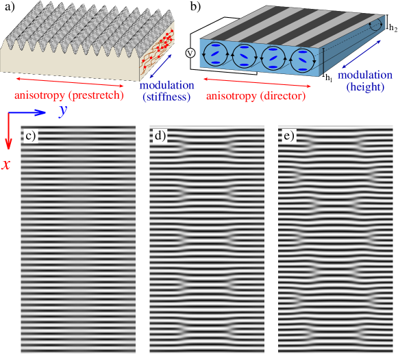
Figure 1: In (a) a wrinkle forming elastic system is sketched with a spatially varying stiffness and in (b) electroconvection in nematic liquid crystals with a spatially varying height of the convection cell. Parts (c)-(e) show selected characteristic patterns for the proposed system class. They are stable at identical parameters and have been obtained numerically via equation (II) for the parameter set $\hat{q}_{0}=1$, $k_{m}=0.05$, $M=0.1$, $\varepsilon=0.08$ and for different initial conditions by using the pseudo-spectral method Kopriva . Each picture is a cutout of a larger domain ($L_{x}=80\times 2\pi/\hat{q}_{0}$ and $L_{y}=2\pi/k_{m}$).

In this paper we identify and analyze a new class of quasi-2D anisotropic inhomogeneous pattern forming systems. The wave vector of the patterns lies close to $\hat{\bf q}_{0}=(\hat{q}_{0},0)$ along the preferred $x$-direction (anisotropy), as for the two experimental systems sketched in figure 1: (a) a spatially modulated version of the wrinkle forming system Groenewold_Rev ; Glatz2015 and (b) a modulated version of electroconvection (EHC) in nematic liquid crystals Kramer:95.1 . By a modulation we break in such systems the translational symmetry along the perpendicular $y$-direction, causing a variation of the pattern’s natural wavenumber $\hat{q}_{0}$. This can be accomplished by varying the elasticity in the wrinkle forming system or the height of the electroconvection cell, respectively. In this class of anisotropic systems we find straight stripes, cf. figure 1(c), that are stable for wavenumbers in a finite range around $\hat{q}_{0}$, similar as in homogeneous anisotropic systems. In addition, however, we find a whole family of stable branched patterns as shown in figure 1(d) and (e). Surprisingly, they have – at identical parameters – different characteristic wave numbers and include different numbers of branching points. Moreover, the branched patterns coexist with the straight stripes in a wide parameter range. This behavior is a non-trivial generalization of the wave number bands (Eckhaus bands) for homogeneous systems Eckhaus:65 ; Zimmermann:85.1 ; Lowe:85.2 ; Zimmermann:85.2 ; Dominguez-Lerma:86.1 ; Riecke:86.1 ; Kramer:1986.1 – a well established concept and experimentally verified e.g. in EHC Lowe:85.2 and axisymmetric Taylor vortex flow Dominguez-Lerma:86.1 ; Riecke:86.1 – to inhomogeneous systems and multiple patterns. In the following we present the universal amplitude equation of this new symmetry class of patterns and analyze its solutions.

II Model and generic amplitude equation

A generic model for the formation of stationary periodic patterns in anisotropic – but homogeneous – 2D systems, described by a field $u(x,y,t)$, has been proposed in Ref. Kramer:1986.1 . One interpretation of the field $u(x,y,t)$ is, that it describes the (small) lateral displacement of a thin elastic plate extended in the $x$-$y$ plane, loaded along the $x$ and $y$ direction and supported by an elastic medium, similar as in wrinkling systems (whereby the in-plane elastic deformations are neglected) Kramer:1986.1 . Here we generalize this model to an inhomogeneous situation by modulating the pattern’s preferred natural wavenumber $\hat{q}_{0}$ along the direction perpendicular to the anisotropy (the $x$-direction),

$$q_{0}(y)=\hat{q}_{0}+M\cos(k_{m}y)\,,$$ (1)

with an amplitude $M$ and a wavenumber $k_{m}$ considerably smaller than $\hat{q}_{0}$. Then the dynamics of the patterns, described by the real field $u(x,y,t)$ is goverend by

$$\partial_{t}u =\left[\varepsilon-\left(q_{0}^{2}(y)+\Delta\right)^{2}\right]u-W\partial_{x}^{2}\partial_{y}^{2}u-c\partial_{y}^{4}u-u^{3}$$

$$\qquad\qquad-2(\partial_{y}u)\partial_{y}\left[q_{0}^{2}(y)]-u\partial_{y}^{2}[q_{0}^{2}(y)\right]\,.$$ (2)

The first line corresponds to the original model in Ref. Kramer:1986.1 and the second line includes contributions due to the modulation $q_{0}(y)$. Equation (II) is a representative of the here-identified symmetry class. It can be directly linked to the elastic wrinkle-forming system via an appropriate rescaling Kramer:1986.1 : $q_{0}^{4}=\frac{\kappa}{\lambda_{1}}$ relates the critical wave number to the bending stiffness $\lambda_{1}$ of the hard layer and the elastic modulus $\kappa$ of the substrate. The control parameter $\varepsilon=\left(1-\frac{\mu_{1,c}^{2}}{\mu^{2}_{1}}\right)q_{0}^{4}$ is related to the critical compression $\mu_{1,c}=2\sqrt{\kappa\lambda_{1}}$. Also note that, similar to the homogeneous version Kramer:1986.1 and the wrinkle system, equation (II) can be derived from a functional as described in the appendix. For the following, we have chosen $W=1$, $c=0.5$ and $\hat{q}_{0}=1$ that favor straight stripes formation parallel to the $y$-direction for the homogeneous case.

Close to the onset of supercritically bifurcating patterns their generic (system-independent) properties may be described by a nonlinear dynamical equation for the complex envelope $A(x,y,t)$, considering $u(x,y,t)=Ae^{i\hat{q}_{0}x}+A^{\ast}e^{-i\hat{q}_{0}x}$ with the scaling $u\propto\varepsilon^{1/2}$ (the star denotes the complex conjugate). This reduction method, the so-called multiple scale analysis, is well established for supercritical bifurcations in 2D homogeneous isotropic Newell:1969.1 ; CrossHo and anisotropic systems Kramer:1986.1 ; Zimmermann:88.3 or 1D inhomogeneous ones Zimmermann:96.3 . Following very closely the appendix in Ref. CrossHo with the same intermediate scaling for time and space one obtains with $M\propto\varepsilon^{1/2}$ and $k_{m}\propto\varepsilon^{1/2}$ via the multiple scale analysis from the system described by equation (II) the generic amplitude equation for the here-identified universality class of patterns in anisotropic systems with a spatially varying natural wave number $q_{0}(y)$:

$$\partial_{t}A =\left[\varepsilon+\xi_{x}^{2}\partial_{x}^{2}+\xi_{y}^{2}\partial_{y}^{2}\right]A-g\lvert A\rvert^{2}A\,$$

$$\qquad-i8\hat{q}_{0}^{2}M\cos(k_{m}y)\partial_{x}A-4\hat{q}_{0}^{2}M^{2}\cos^{2}(k_{m}y)A\,.$$ (3)

Upon derivation from equation (II) one obtains the relations $\xi_{x}^{2}=4\hat{q}_{0}^{2}$, $\xi_{y}^{2}=W\hat{q}_{0}^{2}$ and $g=3$. The generic phenomenon of stripes’ branching, as detailed below, is induced in equation (II) by the term $\propto M\partial_{x}A$. The term $\propto M^{2}A$ mainly leads to quantitative modifications. It should be noted that the first line of equation (II) is exactly the equation for the amplitude of stripe patterns in unmodulated EHC Kramer:1986.1 ; Zimmermann:88.3 , the second anisotropic system suggested for experimental investigations of phenomena described here. For all specific pattern forming systems in the considered universality class, equation (II) can be derived via perturbation techniques from the basic equations (as for example from equation (II)) and it has always the same form — only the coefficients will depend on the specific system. The presented results are obtained via the universal equation (II).

III Results and discussion

The modulation of the natural wavenumber, see equation (1), alters the bifurcation from the basic state ($u=A=0$) towards stationary periodic solutions of the form $A(x,y)=e^{iQx}H(y)$. The stability of the latter and of $A=0$ with respect to small perturbations $v(x,y,t)=v_{1}(y)e^{\sigma t+iKx}+v_{2}^{*}(y)e^{\sigma^{*}t-iKx}$ can be determined via the ansatz $A(x,y,t)=e^{iQx}\left[H(y)+v(x,y,t)\right]$, followed by a linearization of equation (II) with respect to small $v$. An expansion of $H(y)$ and $v_{1,2}(y)$ in Fourier modes results in an eigenvalue problem for $\sigma$, whereby solutions are stable when all eigenvalues have negative real parts. Note that in $v(x,y,t)$ we consider only perturbations along the $x$-direction, as perturbations parallel to the stripes (along $y$) have been numerically found to have no effect.

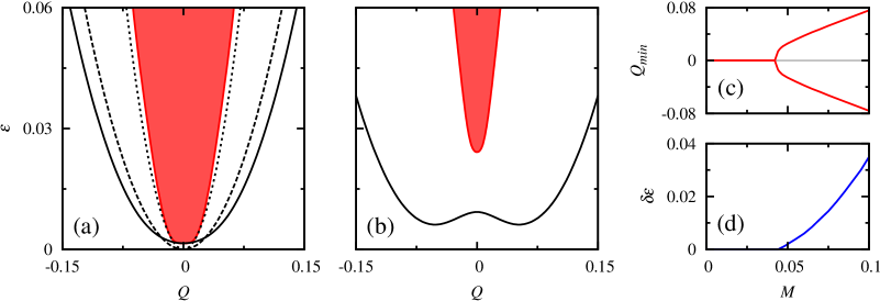
Figure 2: (a) For small modulation amplitude, $M=0.03$, the neutral curve (solid), above which stripes exist, and the Eckhaus stability region (in red), where stripes are stable, have the classical single-well shape with a minimum at $Q=0$. For $M=0$ the neutral (dashed) and the Eckhaus (dotted) curves are given for comparison. (b) With $M=0.075$ beyond a critical value (here $M_{c}\simeq 0.0459$), the neutral curve develops a double-well shape (solid line). The Eckhaus stable region for straight stripe patterns (in red) shrinks and detaches from the neutral curve: a gap develops, where only branched stripes are stable. Within the red region, stable unbranched and branched stripes coexist. (c) The minima of the neutral curve, $Q_{min}$, and (d) the gap $\delta\varepsilon$ between the neutral and the stable range as a function of $M$. Other parameters: $\hat{q}_{0}=1$ and $k_{m}=0.1$.

For the basic state $A=0$ the stability condition, $\Re\left[\sigma_{max}(\varepsilon,Q)\right]=0$, determines the neutral curve $\varepsilon_{\rm N}(Q)$, above which stationary periodic solutions, $A=e^{iQx}H(y)$, of finite amplitude do exist. The neutral curves for the unmodulated case $M=0$ and for a small modulation $M=0.03$ are plotted in figure 2(a) with dashed and solid lines, respectively. Both curves have their minimum at $Q=0$ and are symmetric. However, when increasing $M$, the value of the minimum $\varepsilon_{N}(0)$ shifts towards positive values due to the term $\propto M^{2}A$ in equation (II) that becomes larger ($\varepsilon\rightarrow\left[\varepsilon-4\hat{q}_{0}^{2}M^{2}\cos^{2}(k_{m}y)\right]$). By increasing $M$ further beyond a critical modulation (here $M_{c}=0.0459$ for $\hat{q}_{0}=1$ and $k_{m}=0.1$) a very important phenomenon takes place: The neutral curve develops two minima at finite wave numbers $Q=\pm Q_{min}$, as shown in figure 2(b) by the solid line. The appearence of these two minima is caused by high modulation amplitudes and mainly by the term $\propto M\partial_{x}A$ in equation (II). The dependence of $Q_{min}\propto\sqrt{M-M_{c}}$ on the modulation in the vicinity of $M_{c}$ resembles a pitchfork bifurcation, cf. figure 2(c). The two new terms in the amplitude equation, caused by the modulation, hence widen the neutral curve at small modulations and change its shape from a single- to double-well shape via a pitchfork-like bifurcation at higher modulations. The fact that the modulation along the y-direction causes two minima of the neutral curve $\varepsilon_{N}(Q)$, with respect to $Q$ along the $x$ direction, is crucial for the emergence of branched patterns.

Periodic solutions in the homogeneous case, $M=0$, have a constant amplitude, $H(y)=\sqrt{(\varepsilon-\xi_{x}^{2}Q^{2})/g~{}}$, and they are linearly stable only above the dotted line in figure 2(a), the so-called Eckhaus-stability boundary $\varepsilon_{E}(Q)$. Note that for 2D anisotropic systems, the $Q$-range of stable solutions is symmetric with respect to $Q=0$ Kramer:1986.1 , in contrast to isotropic systems, in which the zig-zag instability occurs for $Q<0$. For small modulations $M<M_{c}$, $H(y)$ is $2\pi/k_{m}$-periodic along the $y$-direction and corresponds to modulated stripes as shown in figures 1(a) and 3(a),(b). In general, the equation for $H(y)$ may have further solutions as well. However, simulations did not show them, so they are either unstable or have higher energies. The Eckhaus stability range of the modulated stripes is qualitatively unchanged compared to the homogeneous limit, as shown by the red-colored region in figure 2(a): It still touches $\varepsilon_{N}(Q)$ at $Q=0$. However, quantitatively, the modulation tends to narrow the width of the Eckhaus-stability range and thus reduces the range of stable stripes.

Concomitant with increasing the modulation beyond the threshold $M_{c}$ a striking change in the stability scenario occurs: i) As shown in figure 2(b), a gap opens between the neutral curve (solid line) and the stability range of amplitude modulated straight stripes (red-colored area). Withhin the gap, the stripe solutions $A(x,y)=e^{iQx}H(y)$ are unstable and thus cannot be observed anymore. The width of this gap increases nonlinearly with $M-M_{c}$, as shown in figure 2(d). ii) Stable branched stripes, like those shown in figures 1(d),(e) and figure 4, emerge within a large area above the neutral curve. iii) Within the red-colored area in figure 2(b), the unbranched modulated stripes coexist with branched stripes at identical parameters sets.

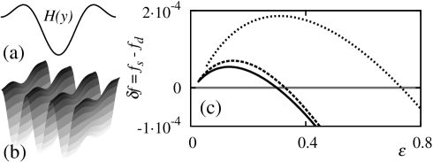
Figure 3: (a) The amplitude $H(y)$ of a modulated stripe pattern given in (b). (c) The energy density difference between the stripe pattern and one of the possible branched patterns, $\delta f=f_{s}-f_{d}$, as a function of $\varepsilon$ for three different wavenumbers [$Q=0$ (solid), $Q=0.0125$ (dashed), $Q=0.025$ (dotted)] within the coexistence region. For small values of $\varepsilon$, branched patterns are energetically preferred, while for large $\varepsilon$ unbranched ones. The crossover position strongly increases with $Q$. Parameters: $\hat{q}_{0}=1$, $k_{m}=0.1$, $M=0.075$.

To characterize the coexistence (the first central result) further, we use the fact that the dynamical equations (II) and (II) can be derived from functionals, which for stationary patterns take the simple form (appendix):

$${\cal F}=-\frac{1}{4}\int dxdy~{}u^{4}=-\frac{3}{2}\int dxdy~{}\lvert A\rvert^{4}\,.$$ (4)

Using the energy density $f={\cal F}/L_{x}L_{y}$ ($L_{x}L_{y}$ is the domain area) one can hence determine which of the stable patterns is energetically preferred at a given parameter set (see also p. 868 of Ref. CrossHo ). We have calculated the energy densities of unbranched patterns $f_{s}$ and of branched patterns $f_{d}$ within the red-colored region in figure 2(b). Their difference $\delta f=f_{s}-f_{d}$ is plotted in figure 3(c) as a function of $\varepsilon$ and for three different wave numbers $Q$. For small $\varepsilon$, branched patterns have a lower energy and thus are energetically preferred, whereas for considerably larger $\varepsilon$, unbranched patterns are in turn preferred. The crossover can be understood as the modulation becomes less important at large values of the control parameter $\varepsilon$.

The second central result is that for each parameter set out of a large range beyond $\varepsilon_{N}(Q)$ we find always a whole family of stable branched patterns, characterized by different wavelengths and distinct numbers of branching points - and obtained by varying the initial conditions. For example, the two patterns in parts (d) and (e) in figure 1 contain five and seven pairs of branching points at identical parameters. They are both stable, however, the value of the functional of every branched pattern is, in general, different. This pattern coexistence in inhomogeneous systems is a surprising generalization of the well established Eckhaus wave number band of stable stripe patterns in homogeneous systems Eckhaus:65 ; Zimmermann:85.1 ; Lowe:85.2 ; Zimmermann:85.2 ; Dominguez-Lerma:86.1 ; Riecke:86.1 . There, stable stripes of different wave numbers coexist at an identical parameter set, as verified in EHC Lowe:85.2 , buckling Zimmermann:85.2 and axisymmetric Taylor vortex flow Dominguez-Lerma:86.1 ; Riecke:86.1 . Here, a band of branched patterns with different wavelengths and numbers of branching points coexists. In both cases, the origin of this coexistence lies in the fact that transitions between two stable periodic patterns require rather high excitations Zimmermann:85.1 worth to be investigated further.

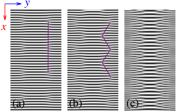
Figure 4: The branched patterns display different arrangements of defects upon increasing the amplitude $M$: (a) Aligned structure for $M=0.06$, (b) Zig-zag order for $M=0.1$, (c) Cascade-like order for $M=0.3$. Parameters: $\hat{q}_{0}=1$, $k_{m}=0.05$, $\varepsilon=0.08$, $L_{x}=80\times 2\pi/\hat{q}_{0}$, $L_{y}=2\pi/k_{m}$.

Another interesting observation is due to the branching points (defects) having opposite topological charges in each half period $\pi/k_{m}$ along the $y$-direction hence they repel each other. As shown in figure 4, this repulsion can lead to different orderings of the defects with increasing defect density, for instance, the zig-zag ordering shown in figure 4(b). It can even lead to more complex cascade-like ordering, as shown in figure 4(c). However, how the detailed ordering of branching points can be controlled by the magnitude, the wavelength and the anharmonicity of the modulation is an interesting and fundamental question that needs to be adressed in the future.

The phenomena identified here are robust and insensitive to the special shape of the imposed modulation of the natural pattern wavenumber. Studying the generic model, equation (II), and imposing instead of a harmonic modulation either an anharmonic wave-number modulation or a step-wise one, we obtain qualitatively the same results Glatz2015 . Consequently, instead of harmonic variations, which may be challenging to implement in experimental systems, a step-like modulations can be used, which is easy to achieve in the wrinkles system by glueing two elastomer substrates with different elastic properties together SchmidtHW:2012.2 ; Glatz2015 .

IV Conclusions

In conclusion, we identified a new symmetry class of pattern forming systems that are anisotropic with a perpendicular modulation. By deriving and analyzing the universal amplitude equation, we showed that this class displays interesting scenarios – the emergence of families of stable branched patterns and their coexistence with unbranched patterns – that we suggest to verify experimentally in two complementary anisotropic systems: First, in wrinkle forming systems Groenewold_Rev , where the elasticity of the substrate [as sketched in figure 1(a)] and/or the thickness of the hard layer on top can be varied perpendicularly to the pre-stretch (anisotropy) direction, as recently realized experimentally SchmidtHW:2012.2 ; Glatz2015 . And second, in dissipative electroconvection in nematic liquid crystals Kramer:96 ; Zimmermann:88.3 ; Kramer:95.1 , where the layer height [as sketched in figure 1(b)] or the driving frequency are modulated perpendicularly to the nematic alignment. For both systems, a thorough theoretical analysis of the modulated basic equations is feasible, including the derivation of the universal equation of the patterns envelope, i.e. equation (II). There is a vast literature on wrinkles recently (see e. g. Refs. bowden ; Groenewold_Rev ; Glatz2015 ; Damman:2010.2 ; He:2012.1 ; Chen:2010.1 ), including control strategies for wrinkle formation, but the question of pattern coexistence seems to have not even been raised yet. Hence studies along the lines proposed here, including quantitative comparisons between theory and experiments, will prove powerful for future control and design strategies, both of unbranched and branched (wrinkle) patterns. Finally, note that the branching of stripe patterns on the skin of fishes Kondo:1995.1 , an important example for patterns in living systems, is probably also induced by inhomogeneities, similar as discussed here, and which are in addition slowly changing with time.

Appendix A Functionals

The dynamical equation Eq. (II) for the field $u(x,y,t)$ can be derived from the functional

$$\mathcal{F}[u(x,y,t)] =\int\tilde{f}(u)dx\,dy=\frac{1}{2}\int\left[-\epsilon u^{2}+\frac{1}{2}u^{4}+W\left(\partial_{x}\partial_{y}u\right)^{2}\right.$$

$$\qquad\left.+c\left(\partial_{y}^{2}u\right)^{2}+\left(q_{0}^{4}(y)u^{2}+2q_{0}^{2}(y)u\Delta u+(\Delta u)^{2}\right)\right]dx\,dy$$ (5)

via the functional derivative

$$\partial_{t}u(x,y,t)=-\frac{\delta\mathcal{F}}{\delta u}=-\left(\frac{\partial\tilde{f}}{\partial u}+\partial_{x}^{2}\frac{\partial\tilde{f}}{\partial(\partial_{x}^{2}u)}+\partial_{x}\partial_{y}\frac{\partial\tilde{f}}{\partial(\partial_{x}\partial_{y}u)}+\partial_{y}^{2}\frac{\partial\tilde{f}}{\partial(\partial_{y}^{2}u)}\,\right).$$ (6)

The functional in Eq. (A) can be simplified by assuming periodic boundary conditions and by using the expression $\partial_{t}u$ from the dynamical equation. One gets

$$\mathcal{F}[u(x,y,t)]=\frac{1}{2}\int\left[\frac{1}{2}u^{4}-u(\partial_{t}u)-u^{4}-2u(\partial_{y}u)\partial_{y}(q_{0}^{2}(y))-u^{2}\partial_{y}^{2}\left[q_{0}^{2}(y)\right]\right]dx\,dy,$$ (7)

where the $-u^{4}$-term compensates for the cubic term occurring in $\partial_{t}u$ and similarly the last two terms. These last two terms again vanish due to the periodic boundary condition (here in $y$-direction):

$$\int\left[-2u(\partial_{y}u)\partial_{y}(q_{0}^{2}(y))-u^{2}\partial_{y}^{2}\left[q_{0}^{2}(y)\right]\right]dx\,dy=-\int\partial_{y}\left[u^{2}\partial_{y}\left(q_{0}^{2}(y)\right)\right]dx\,dy=0\,.$$ (8)

We arrive at the simple expression

$$\mathcal{F}[u(x,y,t)]=-\frac{1}{2}\int\left[\frac{1}{2}u^{4}+u(\partial_{t}u)\right]dx\,dy$$ (9)

and if we are – as in our paper – interested only in stationary patterns, we simply have

$$\mathcal{F}[u(x,y,t)]=-\frac{1}{4}\int u^{4}dx\,dy\,.$$ (10)

Also the amplitude equation (II) can be derived from a functional, which can be simplified for stationary solutions in the same manner, only the prefactor changes:

$$\mathcal{F}[u(x,y,t)]=-\frac{3}{2}\int|A|^{4}dx\,dy\,.$$ (11)

References

- (1) Ball P 1999 The Self-Made Tapestry: Pattern Formation in Nature (Oxford, Oxford Univ. Press)
- (2) Cross M C and Hohenberg P C 1993 Rev. Mod. Phys. 65 851
- (3) Lappa M 2010 Thermal Convection: Patterns, Evolution and Stability (West Sussex, John Wiley and Sons)
- (4) Buka A and Kramer L 1996 Pattern Formation in Liquid Crystals (New York, Springer)
- (5) Bodenschatz E, Zimmermann W and Kramer L 1988 J. Phys. (Paris) 49 1875
- (6) Kramer L and Pesch W 1995 Annu. Rev. Fluid Mech. 27 515
- (7) Feingold G et al. 2010 Nature 466 849
- (8) Goehring L, Mahadevan L and Morris S W 2009 Proc. Natl. Acad. Sci. (USA) 106 387
- (9) Meron E (2012) Ecological Modelling 234 70
- (10) Kapral R and Showalter K 1995 Chemical Waves and Patterns (New York, Springer)
- (11) Mikhailov A S and Showalter K 2006 Phys. Rep. 425 79
- (12) Ben-Jacob E et al. 1994 Nature368 46
- (13) Jalife J et al. 2009 Rotors, Spirals, and Scroll Waves in the Heart, in Basic Cardiac Electrophysiology for the Clinician (Oxford, Wiley-Blackwell).
- (14) Gregor T et al. 2005 Proc. Natl. Acad. Sci. (USA) 102 18403
- (15) Bowden N et al. 1998 Nature 393 146
- (16) Genzer J and Groenewold J 2006 Soft Matter 2 310
- (17) Newell A C, Passot T and Lega J 1992 Annu. Rev. Fluid Mech. 25 399
- (18) Newell A C and Whitehead J A 1969 J. Fluid Mech. 38 279
- (19) Lowe M, Gollub J P and Lubensky T 1983 Phys. Rev. Lett. 51 786
- (20) Coullet P 1986 Phys. Rev. Lett. 56 724
- (21) Zimmermann W et al. 1993 Europhys. Lett. 24 217
- (22) Peter R et al. (2005) Phys. Rev. E 71 046212
- (23) Freund G, Pesch W and Zimmermann W 2011 J. Fluid Mech. 673 318
- (24) Mau Y, Hagberg A and Meron E 2012 Phys. Rev. Lett. 109 034102
- (25) Weiss S, Seiden G and Bodenschatz E 2012 New. J. Phys. 14 053010
- (26) Rehberg I et al. 1988 Phys. Rev. Lett. 61 2449
- (27) Riecke H, Crawford JD and Knobloch E 1988 Phys. Rev. Lett. 61 1942
- (28) Walgraef D 1988 Europhys. Lett. 7 485
- (29) Miguez DG et al. 2004 Phys. Rev. Lett. 93, 048303
- (30) Schuler S, Hammele M and Zimmermann W (2004) Eur. Phys. J B 42, 591
- (31) Hartung G, Busse F H, and Rehberg I 1991 Phys. Rev. Lett. 66 2742
- (32) Schmitz R and Zimmermann W 1996 Phys. Rev. E 53 5993
- (33) Utzny C, Zimmermann W and Bär M 2002 Europhys. Lett. 57 113
- (34) Hammele M and Zimmermann W 2006 Phys. Rev. E 73 066211
- (35) Glatz BA, Tebbe M, Kaoui B, Aichele R, Schedl AE, Schmidt HW, Zimmermann W and Fery A 2015 Soft Matter 11 3332
- (36) Kopriva DA 2009 Implementing Spectral Methods for Partial Differential Equations (Berlin, Springer)
- (37) Eckhaus V 1965 Studies in Nonlinear Stability Theory (New York, Springer)
- (38) Kramer L and W. Zimmermann 1985 Physica (Nonlin. Phenomena) D 16 221
- (39) Lowe M and Gollub J P 1985 Phys. Rev. Lett. 55 2575
- (40) Zimmermann W and Kramer L 1985 J. Phys. (Paris) 46 343
- (41) Dominguez-Lerma M A, Cannell D S and Ahlers G 1986 Phys. Rev. A 34 4956
- (42) Riecke H and Paap HG 1986 Phys. Rev. A 33 547
- (43) Pesch W and Kramer L 1986 Z. Physik B 63 121
- (44) Claussen KU et al. 2012 RCS Adv. 2 10185
- (45) Vandeparre H et al. 2010 Soft Matter 6 5751
- (46) Ni Y, Yang D and He L 2012 Phys. Rev. E 86 031604
- (47) Yin J and Chen X 2010 Phil. Mag. Lett. 90, 423
- (48) Kondo S and Asai R 1995 Nature 376 765