Photoionization analysis of chemo-dynamical dwarf galaxies simulations

Abstract

Photoionization modelling allows to follow the transport, the emergence, and the absorption of photons taking into account all important processes in nebular plasmas. Such modelling needs the spatial distribution of density, chemical abundances and temperature, that can be provided by chemo-dynamical simulations (ChDS) of dwarf galaxies. We perform multicomponent photoionization modelling (MPhM) of the ionized gas using 2-D ChDSs of dwarf galaxies. We calculate emissivity maps for important nebular emission lines. Their intensities are used to derive the chemical abundance of oxygen by the so-called $T_{e}-$ and $R_{23}-$methods. Some disagreements are found between oxygen abundances calculated with these methods and the ones coming from the ChDSs. We investigate the fraction of ionizing radiation emitted in the star-forming region which is able to leak out the galaxy. The time- and direction-averaged escape fraction in our simulation is 0.35–0.4. Finally, we have calculated the total H$\alpha$ luminosity of our model galaxy using Kennicutt’s calibration to derive the star-formation rate. This value has been compared to the ’true’ rate in the ChDSs. The H$\alpha$ -based star-formation rate agrees with the true one only at the beginning of the simulation. Minor deviations arise later on and are due in part to the production of high-energy photons in the warm-hot gas, in part to the leakage of energetic photons out of the galaxy. The effect of artificially introduced thin dense shells (with thicknesses smaller than the ChDSs spatial resolution) is investigated, as well.

1 Introduction

The main information about physical processes and the physical state of the interstellar medium (ISM) in star-forming dwarf galaxies (DGs) are obtained from observed emission line spectra from their nebular components – gaseous nebulae or nebulae surrounding the compact star-forming (SF) region (see the textbooks of Dopita & Sutherland, 2003; Osterbrock & Ferland, 2005).

Line intensity ratios are used to infer the physical state (density, temperature, chemical composition) of ionized regions. These indicators are commonly dubbed diagnostic methods and their use date back to the seventies (Searle, 1971; Pagel et al., 1979), although research is still ongoing in this field (see Pilyugin, 2003; Pettini & Pagel, 2004; Stasińska, 2006). As it is well known, (see e.g. Osterbrock & Ferland, 2005) some intensity ratios (such as [OIII]$\lambda$4363Å  versus $\lambda$4959Å  and $\lambda$5007Å) in range typical for HII regions are much more sensitive to the electron temperature than to electron density, whereas others (e.g. [SII]$\lambda$6716Å/$\lambda$6731Å  and [OII]$\lambda$3729Å/$\lambda$3726Å)  are sensitive to the electron density. In some cases, intensity ratios are very sensitive to both $T_{e}$ and $n_{e}$. In this case, two or more diagnostics must be used at the same time to determine both quantities (see Golovaty et al., 1993; Shaw, 1995). Physical conditions inside nebulae can thus be recovered and, from them, the relative abundances of ions can be determined.

Most of diagnostic methods assume constant electron temperatures and densities as well as ionic abundances over the whole ionized regime, although many attempts can be found in the literature to relax this hypothesis. The assumption of non-uniformity is necessary for instance to explain the discrepancies between electron temperatures found with different diagnostic methods. In particular, the temperature fluctuations are characterized by the so-called $t^{2}$ parameter (Peimbert, 1967). A different approach was proposed by Mathis et al. (1998), who used ratios $f$ between weights of emitting regions to characterize the temperature inhomogeneities. Based on this work, Stasińska (2002) modified the Peimbert’s $t^{2}$ parameter to allow for temperature inhomogeneities in ionized nebulae. However, in all these methods (and in other similar ones), both electron temperature and density in a single ionization zone are assumed to be constant, whereas this assumption is incorrect for most real nebulae, because density, temperature and chemical abundances are all inhomogeneously distributed (see e.g. Tsamis & Péquignot, 2005) for the case of 30 Doradus and Freyer et al. (2003) for models of wind-blown and radiation-driven HII bubbles). Inhomogeneities are much more obvious if we wish to investigate an entire galaxy, where different gas phases, characterized by very different temperatures, densities and metallicities, coexist (see e.g. Walter et al., 2007; Johnson et al., 2012). It is thus necessary to perform a more detailed photoionization modelling of the nebular gas (NG) in DGs that takes into account the spatial variation of physical properties of the gas. We can thus obtain intensity maps of astrophysically relevant emission lines. Using these maps it is possible to calculate the synthetic spectrum of the emission lines along different sightlines.

Emission-line diagnostics are also crucial to infer the correct star-formation rates (SFRs) from galaxies, most commonly from H$\alpha$ emission (Kennicutt, 1998). In fact, Kennicutt’s SFR determination is based on the assumption that photons responsible for the hydrogen ionization stem from the stellar Lyman continuum (Lyc) alone and neglects other contributions as e.g. the cooling radiation of hot bubbles and the excitation from shock-heated regions.

In this paper we illustrate a way to combine detailed chemo-dynamical simulations (ChDSs) of DGs with a state-of-the-art multi-component photoionization model (MPhM), to study the emission properties of star-forming DGs and compare them with observations. The idea is to use the density, temperature and chemical abundances obtained by means of ChDSs at different locations in the DG and to solve (this is the task of the MPhM) the ionizing radiation transfer equation as well as the ionization-recombination, the energy balance, the radiation diffusion equation and the statistical equilibrium equations in different parts of the galaxy, using as physical parameters for each region the results of the ChDS. An additional crucial ingredient is the stellar spectrum, which is provided by running a tailored Starburts99 simulation (Leitherer et al., 1999).

The strategy is thus to run conventional ChDSs and to use the MPhM as a post-process (see also Yajima et al., 2011; Paardekooper et al., 2013; Compostella et al., 2013). The obvious advantage of our approach when compared to radiative hydrodynamical simulations (Yoshida et al., 2007; Krumholz et al., 2012; Hirano et al., 2014) is that the required computational time is very short and that not many assumptions need to be made about radiative transfer. The serious disadvantage of our approach is that the radiation field does not feedback on the hydrodynamics as it should and the energy and pressure in the ChDSs are purely of thermal origin.

This is the first of a series of papers in which we try to extract as many useful information as possible from this combined use of hydrodynamical simulations and photoionization models. In this first paper, we will mainly focus on the details of the MPhM and the synergy between it and the chemo-dynamical simulations. Moreover, we will focus on the escape probability of ionizing photons from our model galaxy, a topic of considerable relevance in the study of the reionization of the universe, as it is believed that DG-sized objects at very large redshifts are the main culprits for the reionization of the universe (see e.g. Vanzella et al., 2012; Kimm & Cen, 2014; Wise et al., 2014), although their contribution is still under debate (see e.g. Fujita et al., 2003). Finally, we will in detail exploit the H$\alpha$ emission from galaxies and the way it has been used in the past to estimate the SFR in galaxies. As mentioned above, we will revise the estimates of SFRs based on the Kennicutt’s H$\alpha$ –SFR relation and we will also offer a possible explanation for the mismatch of H$\alpha$ vs. UV brightnesses (Lee et al., 2009) as proposed by Relano et al. (2012) for galaxies with SFRs of less than $\sim$ 0.01 M_⊙ yr^-1.

The paper is organized as follows: in Section 2 the DG simulations are summarized. In Section 3 the details of the evolutionary models of the SF region are calculated; in particular, the Lyc spectrum due to the DG star formation history is derived. In Section 4 the MPhM is thoroughly described and the results of the photoionization models of different DG angular sectors are analyzed. In particular, we analyze the behavior of intensities of several important emission lines emitted along the different radial directions from the SF region. In Section 5 the numerical scheme for the calculation of the synthetic emission line spectrum (using emissivity maps obtained from MPhM) for any aperture position will be given. Moreover, the ability of different diagnostic methods for the determination of physical parameters and chemical abundances in the NG is tested. In the same Section we consider whether H$\alpha$ is a good indicator of the SFR in galaxies, as it is commonly assumed. In Section 6 we study in detail the escape of ionizing photons from our model galaxy. Moreover, the change in the Lyman continuum spectra due to the intervening hot gas is studied in detail. In Section 7 the most important results of this study are discussed and some conclusions are drawn.

2 Description of the chemo-dynamical simulations

The ChDSs we use in this work are based on the simulations of Recchi & Hensler (2013), hereafter RH13. This work was aimed at simulating dIrrs with different baryonic masses and initial gaseous configurations, in order to study the conditions under which a galactic wind could develop and determine the fate of metals, freshly produced during a SF episode. In all RH13 simulations, the galaxy is assumed to be axially symmetric and rotating about the axis of symmetry, with a frequency that depends only on the distance from the axis $R$ and not from the vertical coordinate $z$, in compliance with the so-called Poincaré-Wavre theorem (Tassoul, 1978). The numerical code solves the 2-D gas-dynamical equations in cylindrical coordinates, using a second-order scheme with flux limiters. The evolution in space and time of various chemical elements (H, He, C, N, O, Mg, Si and Fe) is followed by means of appropriate passive scalar fields. Detailed sources of energy and of chemical elements due to supernovae (SNe) of both Type II and Type Ia and from winds of massive and intermediate-mass stars are taken into account. The details of the numerical scheme and of the implementation of the feedback from dying stars can be found in (Recchi et al., 2001, 2004, 2006).

The set of models of RH13, in spite of the fact that they are not tailored to any specific dwarf galaxy (at variance with the ones of Recchi et al. (2006) for instance), have a much higher spatial resolution and a more accurate description of the chemical feedback than previous simulations of our group. They are thus ideal to illustrate the way in which emissivities can be calculated starting from ChDSs. We will use, as a reference model, the model L8F of RH13, i.e. a model with 10⁸ M_⊙ of baryonic mass and a flat initial configuration. This model develops a nice and undistorted galactic wind (see fig. 4 of RH13). Since one of the aims of our paper is to study the emissivities from galactic wind regions and escape fractions of various photons, this model is ideal for our purposes. We have also studied the emission properties of the model L8M of RH13. This is a model, similar to the reference model L8F, but with a reduced initial degree of flattening. Consequently, a galactic wind develops later in this model compared to model L8F and in a more distorted and turbulent way (see again fig. 4 of RH13). In both models, the SFR is assumed to be constant during the first 500 Myr of galactic evolution and equal to 2.67 $\cdot$ 10^-2 M_⊙ yr^-1. In spite of the differences, the results obtained with model L8M are qualitatively similar to the ones obtained with the model L8F. They are only more difficult to interpret due to the enhanced turbulence, therefore we concentrate on L8F. We do expect significant differences with the roundish model L8R though. A detailed comparison between emissivities and spectra obtained with models L8F, L8M, and L8R will be presented in a forthcoming paper.

A typical map of density and temperature resulting from the ChDS of the model L8F is shown in Figure 1.

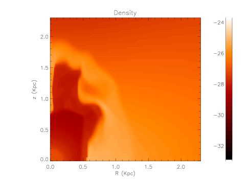
Figure 1: Gas density (upper panel) and temperature (lower panel) maps obtained from the L8F model (see Sect. 2 for details on the ChDS models), calculated at an evolutionary time of 140 Myr. Brighter colors indicate larger gas densities and temperatures.

3 Spectra of the ionizing radiation from stars

The Lyman continuum spectrum originates from the stellar population and then is modified by the intervening gas. In order to set the starting ionizing spectrum, we use tailored Starburst99 (v.7.0.1) simulations. The input SFR matches the one adopted in various ChDSs (see Section 2). The adopted initial mass function (IMF) is the Salpeter one. The Padova AGB evolutionary tracks for Z=0.004 as well as the Maeder wind model were used. We run the Starburst99 simulations for 200 Myr, with timesteps of 1 Myr.

Figure 2: Syntethic radiation spectra from the SF region at different ages

The total number of the ionizing photons $Q_{ion}$ emitted by the SF region per unit time weakly depends on the age. The resulting Lyc spectra at the inner radius of the nebular region are given in Figure 2.

4 The multi-component photoionization modelling

In this section we present the algorithm to perform the multi-component photoionization modelling of NG in DGs. The results of such modelling based on ChDSs, such as the emissivity maps for important emission lines, the transformation of the ionizing Lyc-spectrum and the predicted emission line spectra obtained along various radial directions will be considered as well.

4.1 The MPhM wrapper

As basis for the photoionization modelling we used G. Ferland’s code CLOUDY 08.00 (see Ferland, 2008).

Looking again at the results of ChDSs (see Fig. 1), the first important conclusion we can draw is that the ionizing gas can be divided into two main parts. The first one is the cavity carved by supernova explosions and stellar winds around the SF region (superwind region – SWR). This component contains very rarefied and hot gas. Also the abundance of heavy elements is very high. Since the MPhM does not treat shock-heated gas, the temperature in this region can only be determined by the ChDS. The second component is the supershell swept up by the propagating shock (hereafter called ’wall’). It is characterized by much higher gas densities, as well as by heavy-element abundances typical for the galactic ISM. The ’wall’ corresponds thus to the outer edge of the SWR. It is important to point out that, in spite of the larger densities and the relatively low temperatures, a significant fraction of the wall is ionized because the leakage of ionizing photons from the inner region of the galaxy is significant (see below). Beyond the wall, the gas is unperturbed and it is heated mainly by photoionization. Therefore, the temperature in this component can be obtained as a solution of the photoionization thermal energy-balance equation.

The second important conclusion from the analysis of ChDS results is that the maps of density and temperature are very complex. In spite of the axial symmetry, the whole galaxy can not be approximated by a simple geometrical figure. Therefore, it is impossible to use any of the geometrical shapes offered as options in CLOUDY. Obviously, a more complex strategy to simulate the gas emission is required, in order to take into account the very large variations of density, temperature and chemical composition across the galaxy (see also the Introduction for alternative strategies).

Morisset (2006) (see also references therein) developed the so-called pseudo-3D extention Cloudy_3D of CLOUDY, in order to model the emission of nebular objects in 3D geometry, using many 1D photoionization models. This is an appropriate strategy to model objects like diffuse ionized gas surrounding star-formation regions. Nevertheless, we decided not to use this code and to write our own specialised driver MPhM (multicomponent photoionization modelling) to calculate the multicomponent photoionization models for the following reasons: 1) We are not using the standard CLOUDY release but a customized version. In particular, it was necessary to update the core of CLOUDY to distinguish between SWR and ordinary nebular gas. 2) To generate brightness maps end emission line profiles, Morisset (2006) developed IDL-procedures, but IDL is not a free software and therefore it is not available to all astrophysicists who are interested in such models. Therefore, we developed our own code DiffRay (described below) to calculate the emission line spectra in synthetic apertures with user-defined sizes and positions. We plan to make the MPhM driver as well as the code DiffRay freely available to all the astrophysical community. 3) We are continuously upgrading MPhM (and also the core of CLOUDY) to better adapt it to the study of the nebular emission in galaxies.

In the MPhM approach, the whole computational box of the ChDS is divided into angle sectors, namely solid angles drawn from the origin of coordinates, which is the location of the central star cluster (see Figure 3). As already mentioned, ChDSs are calculated in 2D geometry assuming cylindrical symmetry. This implies in particular that only one quadrant in the $R-z$ plane must be calculated. We divide this quadrant into 20 angle sectors (see Figure 3). In what follows, the sectors will be numbered from 1 to 20, with Sector 1 being the one adjacent to the galactic plane and Sector 20 the one adjacent to the z-axis (the axis of symmetry). Each sector is in turn uniformly divided into 200 radial components. The radial extent of each component is 11.5 pc. The gas at radial distances larger than 2.3 kpc has been considered as part of the intergalactic medium.

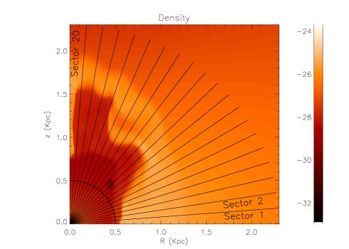
Figure 3: Scheme of the division of the computational box into sectors and components. Sectors are numbered from 1 to 20, with Sector 1 being the one adjacent to the galactic plane (i.e. adjacent to the R-axis) and Sector 20 the one adjacent to the axis of symmetry (i.e. adjacent to the z-axis).

A simple coordinate transformation and an interpolation allow us then to map the ChDS results into the MPhM frame. In particular, in each of the sectors and components, the following input data have been derived and stored

• the hydrogen density;

• the electron temperature (only in the SWR, i.e. in the innermost part of sectors);

• the chemical abundances of 9 chemical elements (H, He, C, N, O, Mg, S, Si, Fe).

It is worth stressing that CLOUDY itself divides the computational volume into zones which are usually smaller than our above defined components. Therefore, CLOUDY performs a further interpolation on the input data.

The edge between hot SWR and wall is defined by the locus of points across each sector where the density gradient is highest. In most of the wall (and also in external regions), the temperature derived from the ChDS is below $\sim$ 4000 K. For these components, we rely on the temperature derived by CLOUDY, as the heating effect due to radiation can be very significant. A detailed analysis of such situation is presented in the following subsection.

In our models, two kinds of ionizing radiation are taken into account. The first is the stellar emission from the SF region. In Fig. 2 the synthetic ionizing radiation spectra are shown, depending on time. The second kind of ionizing radiation is the diffuse one appearing in the NG, mainly due to the radiative recombination onto the ground level of the ions H⁺, He⁺, He⁺⁺, onto the second level of He⁺⁺ as well as by $Ly\alpha$ transitions of HeI and HeII. The diffuse ionizing radiation is calculated using the ”outward-only” approximation, which is the default in CLOUDY. According to this approximation, the diffuse radiation flux from each component, (taking into account all important sources of opacity), is added to the incident continuum flux from the central SF region. The radiation from each component is allowed to propagate only outwards. Thus, each angular sector in the present MPhM approach is ”isolated” from the ionizing radiation from the others. This is clearly a simplification, made in order to reduce the computational costs. More advanced solutions are currently being developed and tested.

We perform MPhM calculations in the time interval from 10 to 200 Myr with timesteps of 10 Myr. At each time step, we take a different ChDS output and a different stellar spectrum, in order to keep pace of the changes occurred in the gaseous and stellar component of the galaxy.

4.2 Photoionization modelling of sectors

As mentioned in Section 2, we will mostly focus on MPhM calculations based on the ChDS L8F. In Fig. 4 the variation of the electron density and temperature across some angular sectors are drawn, as a function of radial distance from the center. Different lines indicate different evolutionary times. As a reminder, Sector 1 runs across the galactic plane, therefore the hole of low density and high temperature (the SWR in our nomenclature) is less extended. Conversely, Sector 19 lies close to the axis of symmetry, i.e. along the direction of steepest pressure gradient. Along this direction a galactic wind develops faster and thus the SWR is more extended (see also Fig. 1).

Figure 4: Variation of the electron density and temperature across some angular sectors, as a function of radial distance from the center. Different lines indicate different evolutionary times. The calculation refers to the ChDS model L8F (see Sect. 2 for details).

In Fig. 4 one can clearly see the edge between the SWR, characterized by high temperatures and low densities, and regions of gas still at lower temperatures and at higher densities. In some cases however some oscillations in the temperature profiles can be discerned, with colder regions preceding hotter ones. This is due to the turbulent nature of the galactic outflows and to the adiabatic cooling of the outflowing gas. This can be clearly seen in Fig. 1. A ridge of shock-heated gas stretches from (R,z) $\simeq$ (0, 2) kpc to $\simeq$ (0.8, 1.5) kpc. This gas has a temperature higher than the background one. Behind it, there is a strip of adiabatically cooled gas. Moreover, a turbulence-generated eddy starts developing at (R,z) $\simeq$ (0.5, 1.4) kpc. It is thus possible that some sectors, at some evolutionary times, intercept regions at different temperatures, generating thus the temperature oscillations visible in Fig. 4. This effect can be particularly significant from Sector 10 onwards. Because of these inhomogeneities in the temperature distribution, we allow CLOUDY to calculate the electron temperature any time the temperature derived from the ChDS drops below 4000 K. It can also be seen that for sector 1, containing the densest and thickest ’wall’ element, the outer ionization front occurs at distances from 0.8 to 1.3 kpc, depending on age. This is the outer ionization front due to the absorption of ionizing photons in the gas. This means that in radial directions of low-number sectors the gas opacity is large and a very small fraction of the ionizing radiation propagates beyond the wall.

The MPhM allows to calculate the emissivity maps for important nebular emission lines, that can be used to calculate the corresponding radiative fluxes along any direction. This is necessary in order to obtain theoretical spectra to compare with observed ones.

Figure 5: Radial variation of the emissivities of the recombination lines H$\alpha$ and $\lambda$ 4686 HeII for selected sectors and ages.

In order to investigate where in the nebula the recombination as well as collisionally excited (forbidden) emission lines arise, we have plotted the radial distributions of line emissivities (see Figures 5 – 6). We have chosen to plot only four representative sectors and not all 20 in order to make the plots clearer. In particular we have chosen the plane sector (sector 1), two central sectors (sectors 8 and 13) and a sector close to the axis (sector 19). We have not chosen sector 20 because axysimmetric hydrodynamical simulations (such as our simulations) unavoidably show some numerical noise along the symmetry axis. In the left panels of Figure 5, the radial distribution of the H$\alpha$ emissivity (as usual, separated into angular sectors) is shown. This line emissivity behaves quite similarly to the electron density (see Figure 4) as expected, because this recombination line has a strong dependence on electron density and a very weak dependence on the electron temperature. For the first seven sectors the emissivities drop at the ionization front, whereas for high-number sectors the external regions of the galaxy are emitting significantly in H$\alpha$ . This is because the optical thickness of the gas is lower and the radiation field (mainly due to Lyc photons from the central SF region) keeps the temperature until $R\sim 1-2.5$ kpc relatively high, with $T_{e}$ ranging between 4000 and 32000 K. The optical thickness for Lyc photons is not high, because the intervening gas has on average relatively low densities (of the order of 0.1 cm^-3). This figure is very low in comparison with typical densities in conventional HII regions, where $n_{H}\ =\ 1-300\ cm^{-3}$. Notice that in spite of the good spatial resolution of our hydrodynamical simulations (4 pc), this is still not enough to resolve HII regions properly (let alone to resolve compact and ultra-compact HII regions) and this is clearly a limitation of our model, as the leakage of Lyc photons in our results is perhaps higher than it should be (see Sect. 6). High-resolution multi-phase simulations are currently being tested, in order to remedy to this situation. In this work, for illustrative purposes, we have decided to make a simpler (and less physically justifiable) hypothesis, namely that a clumpy phase is present in the galaxy at spatial scales that can not be solved by our hydrodynamical code. Therefore, we add this clumpy phase only during the MPhM post-processing (see next Section for more detail).

The behaviour of H$\beta$ and HeI$\lambda$4471 as well as other HeI lines emissivities are also quite similar to the H$\alpha$ . The emissivity of HeII$\lambda$4686 shows the peaks in ’wall’ sectors, corresponding to maxima in the electron density distribution. Again, for sector 1, this emissivity drops to almost zero at the ionization front. This is because the ionization potential of He⁺ is 4Ryd. The ’wall’ absorbs the photons beyond 4Ryd. Therefore, the fraction of the ionizing photons beyond the ’wall’ is very small. Thus, at the inner edge of the ’wall’ one has frequently He⁺⁺/He$>$He⁺/He, but the He⁺⁺/He fraction drops faster than the He⁺/He one. The emissivity of HeII$\lambda$4686 line is only caused by recombination of He⁺⁺. In the wind region (SWR) He⁺⁺/He$\gg$He⁺/He, because the high temperature here prevents the recombination so that there does no significant emissivity in HeII$\lambda$4686 line emerge.

Figure 6: Evolution of the radial distribution of $\lambda$5007[O III] emissivities for selected sectors and ages.

In order to illustrate the behaviour of forbidden line emissivities we show in Fig. 6 the radial distribution of [OIII]$\lambda$5007. This line, like other forbidden lines, is sensitive to the electron temperature. The highest temperature values occur inside the superwind cavity region. Nevertheless, the [OIII]$\lambda$5007 emissivity is very weak, because at such high temperatures the abundance of O⁺⁺ ions is very low (see next Section). As expected, for sector 1, characterized by the presence of an outer ionization front, the [OIII]$\lambda$5007 emissivity drops to almost zero at the ionization front.

5 Synthetic spectra, their analysis, and comparison with observations

Observed emission line spectra from spatially distributed NG surrounding the SF region are usually obtained from different aperture positions (see e.g. Kobulnicky & Skillman, 1997, KS97). Across these apertures, abundances of various chemical elements can be derived by different diagnostic methods. The aim of this section is to compare the chemical abundances directly obtained from ChDSs with the ones obtained after applying diagnostic methods to the MPhM output files. In this way we try to assess the validity of various diagnostic methods, as well as the correctness of our methods and procedures. In fact, as illustrated in the previous Sections, our combined ChDS+MPhM simulations allowed us to produce 3D maps of emission line and continuum emissivities, which we illustrated by means of radial variations across various angular sectors. On the other hand, by means of ChDSs alone we have the spatial distribution of the abundance of nine chemical elements (H, He, C, N, O, Mg, Si, Fe), as a function of time. We thus have all required information to test the diagnostic methods.

In this Section we shortly describe the procedure to calculate the synthetic emission line spectra from different aperture positions using emissivity maps. We firstly define non-central (i.e. along lines-of-sight which do not pass through the center of the DG)) and central aperture positions (see Fig. 7). Synthetic spectra are calculated by integrating the intensity maps across each aperture (see next subsection for more details). Synthetic spectra are in turn used to determine the oxygen abundances using two well-known and widely used diagnostic methods, namely the two-zones $T_{e}$-method (see Pagel et al., 1992; Garnett, 1992) and the $R_{23}$-method. The latter is based on calibrating relationships O/H-$R_{23}$ from McCaugh (1991). Then we present the comparison of the obtained oxygen abundances with the ones from the ChDS for the corresponding aperture.

5.1 Synthetic spectrum calculation

To calculate the emission line spectrum using emissivity maps we developed the 3D code DiffRaY. This code integrates the fluxes in emission lines over the solid angle that is defined by the aperture position relative to the observer position.

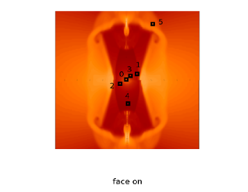
Figure 7: The definition of aperture cuts. The central aperture is labeled by zero. $\alpha$ is the angle between the symmetry axis and the plane normal to the observer sight line. The left panel is the side view of the object. The right panel is the front view. Here, the size of the aperture can be appreciated.

We consider each aperture not as an infinitesimally thin needle, but as a geometrical figure having a section of 49 pc $\times$ 49 pc. This section area is further subdivided in $n\times n$ smaller volumes. The subdivision process is iterative and $n$ represents the stage of the iteration. $n$ is equal to four in the first iteration. At each stage of iteration, the radiative fluxes are integrated across each subdivision of the aperture. Among different possible numerical integration techniques (see Press et al., 1992), we have chosen the trapezoid method, as it is the optimal choice for this kind of problems (see Buhajenko & Melekh, 2013). The code repeats this procedure, increasing $n$ by 2 at each step, and iterates until convergence, i.e. until the differences between line intensities at two different stages of iteration are less than 2 %.

We tested this code by comparing the radial line fluxes obtained from this 3D integration program with the ones obtained by CLOUDY. In Table 1 the ratios between our results and CLOUDY’s ones are given. It can be seen that these ratios are always very close to unity, with deviations of $\sim$ 1.7% at most.

5.2 Synthetic spectra from different aperture positions

In order to test the ability of the two-zones $T_{e}$-method (Pagel et al., 1992; Garnett, 1992) and $R_{23}$-method (Pagel et al., 1979) to determine the oxygen abundances in galaxies, we calculated synthetic emission line spectra using MPhM emissivity maps, as described above.

The angle $\alpha=30^{o}$ (see Fig.7) characterizing the inclination of the galaxy relative to observer was adopted.

Table 1: The ratios between radial fluxes, calculated by our 3D integration program DiffRaY and the ones obtained by CLOUDY for the sectors 1, 8, 13, and 19.

Line	Sector 1	Sector 8	Sector 13	Sector 19
H$\beta$	0.985	1.002	1.002	0.985
H$\alpha$	0.985	0.994	0.997	0.995
Ly$\alpha$ $\lambda$1216	0.984	1.011	0.991	0.983
$\rm[OII]\lambda$3729	0.998	1.003	0.999	0.990
$\rm[OII]\lambda$3726	0.999	0.992	0.998	0.998
$\rm[OIII]\lambda$5007	0.984	0.990	0.996	1.003
$\rm[OIII]\lambda$4363	1.000	0.994	1.000	0.979
HeI $\lambda$4471	0.998	0.991	0.989	0.993
HeI $\lambda$5876	0.994	0.991	0.995	1.004
HeI $\lambda$6678	0.995	0.996	1.006	1.002
HeI $\lambda$7065	0.987	0.991	0.993	0.994
$\rm[SII]\lambda$6716	0.988	1.002	1.008	0.984
$\rm[SII]\lambda$6731	1.004	0.992	0.993	1.000
$\rm[NII]\lambda$6548	0.989	0.995	1.004	1.001
$\rm[NII]\lambda$6584	0.989	0.996	1.004	1.000

5.3 Comparison of modelled and observed emission line spectra

The aim of this subsection is to compare the calculated relative line intensities with the observed ones. For this comparison with observations we use the sample of selected observed spectra from Kehrig et al. (2004). From this sample, we selected galaxies with H$\alpha$/H$\beta$ between 2.6 and 3.2, because our models results are in this range (see Figure 8). The resulting observational ranges for the intensities of important emission lines are given in column 2 of Table 2. Of course, we do not expect a perfect match between theoretical expectations and observations, because this paper is not intended for this purpose, but model emission line intensities should be the of the same order as observed ones.

Figure 8: The evolution of H_α/H_β for six synthetic aperture positions (AP).

In Table 2 and in what follows, we label with M1 the standard model, i.e. the analysis done starting from the results of the ChDS. Model M2 refers to a modification of the ChDS results, in which a very thin shell of enhanced density is artificially added (see below for more detail).

Table 2: Comparison of relative line intensities observed at galaxies, selected from the sample of Kehrig et al. (2004) with derived ones of models M1 and M2 (see text).

Relative intensity	Observed	M1	M2
	range
${\rm[OIII]}{\lambda 5007}/{\rm H\beta}$	0.58 .. 7.84	2.08	3.47
${\rm[OIII]}{\lambda 4363}/{\rm H\beta}$	0.03 .. 0.15	0.03	0.03
${\rm[OII]}{\lambda 3727}/{\rm H\beta}^{*}$	0.40 .. 7.19	0.18	1.95
${\rm[OIII]}{\lambda 5007}/{\rm[OII]}{\lambda 3727}$	0.17 .. 4.8	11.6	1.78
${\rm[SII]}{\lambda 6716}/{\rm H\beta}$	0.05 .. 0.66	0.02	0.23
${\rm[SII]}{\lambda 6731}/{\rm H\beta}$	0.04 .. 0.76	0.02	0.16
${\rm H\alpha}/{\rm H\beta}$	2.63 .. 3.18	2.95	2.93
${\rm[NII]}{\lambda 6584}/{\rm H\alpha}$	0.02 .. 0.29	0.001	0.025
${\rm[SII]}{\lambda 6716}/{\rm H\alpha}$	0.02 .. 0.21	0.007	0.08
${\rm[SII]}{\lambda 6731}/{\rm H\alpha}$	0.02 .. 0.25	0.007	0.06
$\rm[SII]({\lambda 6716}+{\lambda 6731})/{\rm H\alpha}$	0.03 .. 0.46	0.01	0.13

${}^{*}{\rm[OII]}{\lambda 3727}/{\rm H\beta}={\rm[OII]}(\lambda 3726+\lambda 3729)/{\rm H\beta}$

Figure 9: Some important line intensities, obtained for six synthetic aperture positions (AP), as a function of time: a) [OIII]$\lambda 5007$ – one of the main coolers of nebular gas, also used in diagnostics for oxygen abundance determination; b)[OIII]$\lambda 4363$– important line for electron temperature determination; c) [OII]$\lambda 3727$ – it is a sum of [OII]$\lambda 3726$ and [OII]$\lambda 3729$ line intensities, that are important to determine the oxygen abundance; d) [SII]$\lambda 6716$ – the ratio of this line to [SII]$\lambda 6731$ is used in diagnostic for electron density determination. The intensities are normalized to $I_{\rm H\beta}$. To compare with observations the minimal value, obtained from observed emission line spectra of galaxies, selected from sample by Kehrig et al. (2004) are shown by solid lines (Min.obs.) in each panel.

In Figures 9 the time dependences of the relative line intensities (relative to H$\beta$) of important emission lines, obtained for various synthetic aperture positions (see Fig. 7) are shown. It can be seen that our models predict [OIII]$\lambda 5007$ (see Fig. 9a)) line intensities higher than the observed minimum or very close to the one for most of APs. Only in the case of AP 4 intnesity of this line is higher than the observed minimum after 120 Myr. The relative intensities of [OIII]$\lambda 4363$, [OII]$\lambda 3727$ and [SII]$\lambda 6716$ (see Fig. 9b–d) ) for most of ages and APs are not able to reproduce the observed minimum.

To further simplify the comparison of the model results with observed ones, we select the relative intensities obtained as a function of radial distance of sector 1 at 140 Myr. The resulting intensities are given in column M1 of Table 2. This angular sector has the same problems shown by the aperture positions above, i.e. it severely underpredicts the [OII]$\lambda 3727$ and [SII]$\lambda 6716$ emission line intensities. We also compare the intensities of ${\rm H\alpha}/{\rm H\beta}$, of [NII]$\lambda 6584/{\rm H\alpha}$, and of the sum of [SII]$\lambda 6716/{\rm H\alpha}$ and [SII]$\lambda 6731/{\rm H\alpha}$ with observed ones. It can be seen that only the values of ${\rm[OIII]}{\lambda 5007}/{\rm H\beta}$, ${\rm H\alpha}/{\rm H\beta}$ and ${\rm[OIII]}{\lambda 4363}/{\rm H\beta}$ are within the observed ranges. The other line ratios are underestimated in model M1.

The difficulty in reproducing the correct [OII] and [SII] intensities boils down in the end to the relatively low gas density across most of the computational volume; a limitation of the model we have already outlined in the previous Section. Due to this low density, the temperature beyond the ’wall’ in most cases is relatively high. This prevents the formation of a significant fraction of ${\rm O^{+}}$ ions. In this part of the galaxy, the oxygen is in fact mostly doubly ionized and this explains the reasonable agreement between [OIII] intensities and observations. To illustrate this point, the various ionization stages of oxygen across the wall at t=140 Myr are shown in Fig. 10, upper-left panel. We have chosen the angular sector 1 (i.e. the one adjacent to the plane of the galaxy, see previous Section), between 0.5 and 0.75 kpc because the radial distribution of the various ionization stages can be better appreciated.

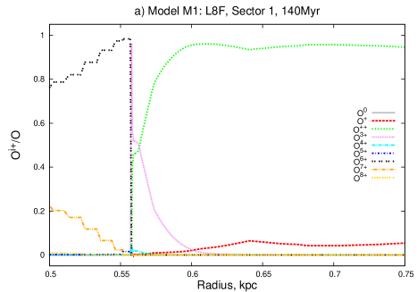
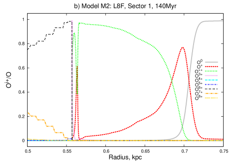
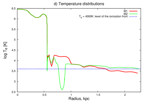
Figure 10: Radial distribution of the oxygen ionization fractions, hydrogen densities and electron temperatures in Sector 1 at 140 Myr in models M1 and M2. Model M2 is characterized by the addition of a thin shell of enhanced density in ’wall’ with a peak density of $7cm^{-3}$ (for comparison, the standard density obtained from ChDS at this position is about $0.2cm^{-3}$).

In order to address the problem of the lack of very dense regions in our computational volume, we decided to introduce one dense shell of enhanced density (TDS – thin dense shell). This TDS represents a thin density enhancement, due to a shock, impossible to resolve with the currently adopted numerical resolution. The shell extends for 10 pc (see Fig. 11) and reaches a peak density of $n_{H}=7cm^{-3}$. This peak density (not the entire shell; just the peak) extends for 1 pc. The M1 density at the peak position is instead about $0.2$ cm^-3. With such a background density, the TDS peak density would thus represent a density enhancement of $\sim$ 35 in a shock. For a strong isothermal shock, this would correspond to a Mach number of $\simeq$ 6 (for instance see the textbook of Draine, 2011), perfectly reasonable under the studied conditions.

To illustrate the effect of the TDS presence we have chosen again Sector 1, because it is the sector adjacent to the plane of the galaxy, where the presence of a TDS is more likely. The TDS inherits the chemical composition of the underlying material. We calculated models of Sector 1 that differ by the position of this TDS: at the wall; midway between the wall and the outer radius of the considered computational box ($R_{out}\approx$ 2.3kpc); and very close to $R_{out}$. Only in the case of a TDS positioned in the wall we obtained relative intensities in agreement with observations. The results of this model, labelled M2, are shown in Table 2. Also, in Figure 10 (upper-right panel) the various ionization stages of oxygen for M2 are shown. The TDS produces a significant increase of the ${\rm O^{+}/O}$ ratio at a distance larger than 0.55 kpc. Now, the radial profile of of ${\rm O^{+}}$ in model M2 is more complicated (there are two maxima). This is enough to significantly increase the [O II] and [S II] emission. The disagreement with the observations disappears for M2 (see again Table 2). The values of $I_{\rm H\alpha}/I_{\rm H\beta}$, $I_{\lambda 6584}{\rm[NII]}/I_{\rm H\alpha}$ as well as $(I_{\lambda 6716}{\rm[SII]}+I_{\lambda 6731}{\rm[SII]})/I_{\rm H\alpha}$ are within the observed range too.

The combination of $I_{\lambda 5007}{\rm[OIII]}/I_{\rm H\beta}$ and $I_{\lambda 6584}{\rm[NII]}/I_{\rm H\alpha}$ allows us to place our models in the so-called BPT diagram (Baldwin et al., 1981), the famous seagull-shaped diagram able to distinguish between HII regions due to star formation and AGNs. For model M2 $(\log\ I_{\lambda 6584}{\rm[NII]}/I_{\rm H\alpha}\ ,\ \log\ I_{\lambda 5007}{\rm[OIII]}/I_{\rm H\beta})=(-1.14,0.54)$. Comparing these values with fig. 5 of Baldwin et al. (1981), it is clear that model M2 is well within the HII regions. Our results obey pretty precisely eq. 8 of the Baldwin et al. paper.

In the SWR, the oxygen is present in ${\rm O^{3+}}$, ${\rm O^{4+}}$ and even higher ionization stages, because of the high temperatures. The density and temperature distributions for models M1 and M2 as well as the temperature level of the ionization front are shown in Figure 10 (panels c and d). Because of the TDS, the temperature drops significantly below the ionization front, at distances of the order of 0.7–0.9 kpc. At larger distances, the temperature increases again, because of the reduced density. By means of the TDS, we are thus able to create a layer of neutral gas between two ionized regions.

In the M1 model, the oxygen at large radii exists mainly in the ${\rm O^{2+}}$ ionization stage, therefore the ${\rm O^{+}}$ abundance is too low to reproduce the observed [OII] line intensities. The presence of the TDS (model M2) leads to the appearance of two regions of enhanced by ${\rm O^{+}}$ fractional abundance: the first one is a thin region at the inner edge of the wall; the second one extends up to $\approx$ 0.73 kpc. These ${\rm O^{+}}$ shells are enough to reproduce the observed [OII] emission in observed range (see the results of model M2 in Table 2).

Although the results of model M2 are encouraging, it is important to point out that our results are quite sensitive to the TDS position and also to the density profile within the TDS. It must be also emphasized that, in our models, diffuse ionizing radiation (emitted by ionized diffuse gas) is calculated in outward only approximation. Therefore, as already outlined, ionizing photons from neighbor sectors cannot penetrate. Therefore, the propagation of the ionizing radiation extends up to the outer ionization front, that occurs at $\approx$ 1 kpc. Such a restriction for the propagation of ionizing photons does not exists in real galaxies. We are working on an extension of the MPhM code to deal with this kind of non-radial propagation of ionizing photons. Such extension is especially necessary to include compact, non-axisymmetric clumps in the model, and to consider spatially extended and non-spherical sources of ionizing radiation.

5.4 Diagnostics of synthetic emission line spectra

Our study aims also at comparing the derived oxygen abundances with the ChDS ones, by means of two popular diagnostics, the $T_{e}$-method and the $R_{23}$-method.

According to $T_{e}$-method (see Pagel et al., 1992; Garnett, 1992), for the determination of the oxygen abundances, we also need the relative intensities of [OIII]($\lambda 4363$,$\lambda 4959$,$\lambda 5007$), and [OII]($\lambda 3726$,$\lambda 3729$), obtained from the synthetic emission line spectra and calculated above for different aperture positions.

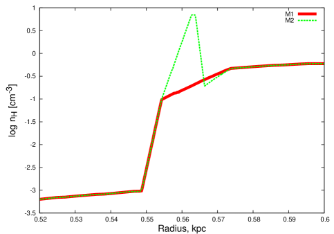
Figure 11: Modification of density distribution in model M2 in comparison with standard model M1 calculated at 140Myr.

However, frequently the emission line $\lambda 4363$[OIII] is absent in real observed spectra, because of low intensity. In such cases the so-called calibration methods are used. In such methods the relationships between (12 + log O/H) and the parameter $R_{23}=(I_{\rm[OII]\lambda 3726+\lambda 3729}+I_{\rm[OIII]\lambda 4959+\lambda 5007})/I_{\rm H\beta}$ are determined on the basis of appropriate calibrations. We select for our tests the calibration of McCaugh (1991).

In Table 3 we compare the oxygen abundances, the luminosity-weighted (L-W) and mass-weighted (M-W) with the ones calculated for the six selected synthetic apertures, using the chosen diagnostic methods, for three different ages. The behaviour of O/H abundances along sight lines becomes more complicate with age. The $T_{e}$-method reproduce the L-W values within an error ($\Delta$) of only 0.5 dex for three APs at 10 Myr, for one AP at 70 Myr and for two APs at 140 Myr. Larger deviations from L-W results can be explained by the inhomogeneous distribution of $\rm O^{+}$ and $\rm O^{++}$ ions. Also, the $R_{23}$-method does not reproduce the oxygen abundance in AP 5. In most cases, the $R_{23}$-method overestimates the oxygen abundances with deviations of more than 0.5 dex, but for some apertures, the L-W abundances are very close to the ones calculated with the $R_{23}$-method.

These results show that the considered diagnostic methods cannot be used to precisely determine the oxygen abundance in DGs due to both the inhomogeneity of the element abundance and the very low density ($\leq$3cm^-3 in some cases). The results show also that the model limitations, already pointed out above, might render our model galaxies quite different from real galaxies. In particular, as already pointed out, due to the low density, the optical thickness for the emission lines along most of sight lines are low (probably lower than in real galaxies).

Also in Table 3 (last two rows) we compare L-W and M-W oxygen abundances with the ones determined using both $T_{e}$- and $R_{23}$-methods for models M1 and M2 at 140 Myr. It can be seen that for M1 the difference between the $T_{e}$ and the $R_{23}$ method amounts to 0.4 dex. The differences between the L-W value and the results of $T_{e}$ and $R_{23}$ methods are slightly larger (a bit more than 0.5 dex). Model M2 shows instead a good agreement of the oxygen abundances determined by diagnostic methods with both L-W and M-W determinations. In this case, the $T_{e}$ and $R_{23}$ methods can be used for the determination of the oxygen abundance.

Thus, we can conclude, that $T_{e}$- and $R_{23}$-methods have limitations in two circumstances: $(i)$ in the low-density limit in nebular enviroments with complex element abundance distributions along sight line; $(ii)$ when an additional radiation field contributes to the stellar radiation, as e.g. the cooling radiation of a hot plasma like the superwind bubble. It is clear that a more detailed and punctual analysis of the diagnostic methods can be done only once our models are able to reproduce more faithfully the real physical characteristics of galaxies. Notwithstanding these limitations, we believe that the preformed test is reasonable - we try to analyze the galaxy with the “eyes of an observer” and try to recover the galactic properties from observational methods. At some level what we “get out” should match what we “put in”. Moreover, since we use two different diagnostic methods, we expect at least some agreement between them. The failure to match these expectations entitles us to conclude that diagnostic lines have limitations in low-density, chemically complex regions.

Table 3: (12 + log O/H) values obtained for the ChDS model weighted by luminosity (L-W) and mass (M-W), respectively, and compared to abundances derived by means of the $T_{e}$ and the $R_{23}$ diagnostic methods. The two lowermost lines give the (12 + log O/H) abundances for both analytical model distributions M1 and M2 at 140 Myr, respectively.

Age,	AP	Weighted, from ChDS		Diagnostic methods
Myr		L-W	M-W	$T_{e}$	$R_{23}$(McCaugh)
10	Central	7.90	7.80	6.90	6.48
10	1	7.14	7.23	7.16	6.80
10	2	7.70	7.58	7.27	7.01
10	3	7.89	7.74	6.96	8.98
10	4	5.78	5.78	5.84	6.91
10	5	5.78	5.78	7.01	6.67
70	Central	8.52	8.38	7.38	6.72
70	1	8.29	8.29	6.84	6.61
70	2	9.13	9.09	6.96	9.06
70	3	8.51	8.37	7.48	9.01
70	4	5.77	5.78	5.84	6.92
70	5	5.78	5.78	6.95	6.73
140	Central	8.93	8.98	8.05	8.91
140	1	7.79	8.22	7.42	6.97
140	2	8.51	8.53	7.44	8.99
140	3	9.00	9.03	7.91	8.94
140	4	8.44	8.43	8.35	8.82
140	5	5.78	5.78	7.38	6.88
140	M1	8.07	7.78	7.51	7.11
140	M2	8.21	7.79	8.10	7.96

5.5 The empirical determination of the star formation rate in galaxies

We conclude this section with an estimate of the reliability of empirical indicators for the star formation rates in external galaxies. One of the most commonly used proxy of SF in galaxies is the H$\alpha$ emission. In particular, the calibration of Kennicutt (1998)

$${\rm SFR}\,({\rm M}_{\odot}{\rm yr}^{-1})=\frac{L(H\alpha)}{1.26\times 10^{41}\,{\rm ergs}\,{\rm s}^{-1}},$$ (1)

(based on the Salpeter IMF) is very widely used. Since we are able to calculate the H$\alpha$ luminosity by means of the MPhM code, we are in the condition to compare the SFR based on $L({\rm H\alpha})$ with the ’true’ SFR, i.e. the rate which has been used as input for our ChDS (equal to 2.67 $\cdot$ 10^-2 M_⊙ yr^-1, see Sect. 2). This comparison is shown in Fig. 12.

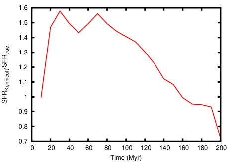
Figure 12: The ratio of the star-formation rate determined from $L({\rm H\alpha})$ (see Eq. 1) and the ’true’ rate, i.e. the rate which is used as input from our ChDS (2.67 $\cdot$ 10^-2 M_⊙ yr^-1) of model M1.

We can see from this figure that, at the beginning, there is a perfect match between the H$\alpha$ -based and the ’true’ SFR. This reassures us about the correctness of our procedures and the accuracy of the Starburst99 code. At later times, however, the H$\alpha$ luminosity increases due to the contribution of the warm gas. The Kennicutt SFR estimates becomes thus inaccurate. It overestimates the true SFR by up to 60 % at t=30 Myr. After 160 Myr, Lyc photons begin to leak out of the galaxy (see Sect. 6), thus the global H$\alpha$ luminosity decreases and the relation Eq. 1 starts underestimating the true SF rate. An accurate study of the status of the gas in a galaxy is thus a fundamental prerequisite in order to assess the reliability of the SF rate estimate based on H$\alpha$ emission. Given the model limitations, an agreement between model results and expectations within a factor of two should be considered as fair. Still, we believe it is important to quantify these inconsistencies and to outline which physical processes can lead to inaccuracies in the Kennicutt’s SFR determinations based on H$\alpha$ emission.

6 The escape fraction of the ionizing photons

In this Section, we investigate how many ionizing photons escape the galaxy volume. These photons could play a fundamental role in the reionization of the Universe (Vanzella et al., 2012; Kimm & Cen, 2014; Wise et al., 2014).

Let the escape fraction of ionizing photons from sector $i$ be defined as follows

$$f_{esc}(i)=\frac{Q_{esc}(i)}{Q_{stars}(i)}=\frac{\int_{\nu_{1Ryd}}^{\infty}\frac{F_{\nu}(esc,i)\ d\nu}{h\nu}}{\int_{\nu_{1Ryd}}^{\infty}\frac{F_{\nu}(stars,i)\ d\nu}{h\nu}},$$ (2)

where $Q_{esc}(i)$ denotes the rate at which ionizing photons leave sector $i$ through the outer edge (i.e. propagate above 2.3 kpc); $Q_{stars}(i)$ is the rate of incident ionizing photons emitted by the stars contained in sector $i$; $F_{\nu}(esc,i)$ and $F_{\nu}(stars,i)$ are the corresponding fluxes of ionizing radiation. It must be noted that $F_{\nu}(stars)$ is not attenuated by the intervening gas; it is the overall flux produced by all central stars. In practice, we perform an integration of both ionizing fluxes over the photon energy range $(1-10)Ry$ for $F_{\nu}(stars)$, and $(1-180)Ry$ for $F_{\nu}(esc)$, respectively. This is due to the fact that $F_{\nu}(stars,i)$ (calculated, as mentioned above, using Starburst99) drops to zero beyond $10Ryd$, but the escape radiation ($F_{\nu}(esc,i)$) contains also the photons at higher energies, emitted by the hot rarefied gas in the SWR. Notice also that high-energy Lyc photons are less absorbed, because the photoionization cross section decreases with photon energy increasing.

The total escape fraction of the ionizing photons is defined as

$$f_{esc}=\frac{\sum_{i=1}^{20}Q_{esc}(i)}{\sum_{i=1}^{20}Q_{stars}(i)},$$ (3)

i.e. we simply sum up all the escape fractions, in all sectors.

In Figure 13 the evolution of $f_{esc}$ for sectors 1, 10, and 18 as well as the total escape fraction is shown. As expected, lower values of $f_{esc}$ belong to low-number sectors, closer to the disk of the galaxy. The escape fraction of ionizing photons for the M2 model are in general very low (of the order of 0.01). Only the escape fraction for sector 18 (close to the symmetry axis) is significantly larger than 0, at least until 50 Myr. This is thus the only result we show for model M2 (see filled squares+dot-dashed curve in Fig. 13).

Figure 13: Evolutionary dependences of the escape fraction $f_{esc}$ of ionizing photons for sectors 1, 10 and 18 as well as for total escape fraction (see text). Also, the evolution of $f_{esc}$ for the model M2 (Sector 18) is shown. The values of $f_{esc}$ for the M2 model along Sectors 1 and 10 are $\approx$ 0.01 at all ages, thus have not been shown.

We can notice from Figure 13, that $f_{esc}$ for Model M1 is on average 0.4. This value is slightly higher than the value found in radiative hydrodynamical simulations (Kimm & Cen, 2014; Wise et al., 2014). On the other hand, model M2 produces much lower values for $f_{esc}$, lower than predicted by simulations and also lower than the values required to ensure that DGs are significant for the reionization of the Universe. Fujita et al. (2003) e.g. found that for DGs with SF efficiencies, i.e. the gas fraction converted into stars above 6%, $f_{esc}$ can be larger than 0.2 and this value is large enough for a significant contribution to the ionizing UV background. Notice however that the true SF efficiency in DGs could be smaller than 6%. In this case, DGs can not be the main responsible for the reionization of the universe. In the model L8F considered here, this SF efficiency is about 13%, thus our average $f_{esc}$ of $\sim$ 0.4 is consistent with Fujita’s calculations.

As we have shown above, the small scale TDS, characteristic of the M2 model, is necessary to reproduce the observed emission line spectra. Of course, in the presence of many TDSs in the DG, the total $f_{esc}$ would be further reduced. However, we shall not forget that our calculations are based on the outward-only approximation and it is possible that a fraction of the ionizing photons are emitted in non-radial directions. This would enhance the $f_{esc}$ in model M2. It appears that some modifications in our modelling procedures (in particular, the relaxation of the outward-only approximation) are required in order to obtain $f_{esc}$ values closer to realistic ones and less dependent on model assumptions.

We also studied the changes of the energy distribution in the ionizing spectrum. For both M1 and M2 models, we show only results relative to sector 1. In Figure 14a) we compare 1) the incident Lyc-spectrum from central stars in the energy range $(13-140)eV$ for both models; 2) the spectrum of the radiation escaping the SWR; 3) the spectrum calculated at the outer edge of galaxy, predicted by model M1. The outer part of the galaxy absorbs very efficiently ionizing quanta in this photon energy range, because of the high density in Sector 1. Therefore, an outer ionization front is present in this sector. The Lyc spectra at the outer edge are very weak. Nevertheless, gaps in the Lyc spectra, mainly positioned at important ionization potentials of ions, are clearly distinguishable. Similar gaps were predicted by optimized photoionization models of HII regions in low-metallicity starburst galaxies (see e.g. Melekh, 2006, 2007). As a result of these models, the optimal Lyc-spectra for HII regions in the blue compact galaxies SBS 0940+544 and SBS 0335-052 was found. The gaps appear also in models of superwind bubbles (Koshmak & Melekh, 2013, 2014).

As mentioned above, the incident Lyc spectrum from stars drops to zero at photon energies $\geq 136eV$ (see Figures 14a,b), but the emission of warm-hot gas contributes photons at higher energies. The spectra in the range $(0.01-1)keV$ are shown in Figure 14b.

It can be seen that the density distribution in the outer part of galaxy (from ’wall’ up to outer edge of the modelling volume) shapes the spectra up to photon energies of $(0.4-0.5)keV$. The spectrum at larger photon energies is practically undisturbed, because of low the optical thickness for these photons. Therefore, the modelled spectrum in this energy range can be compared with X-ray observations.

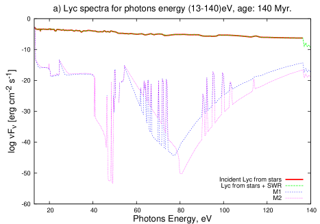
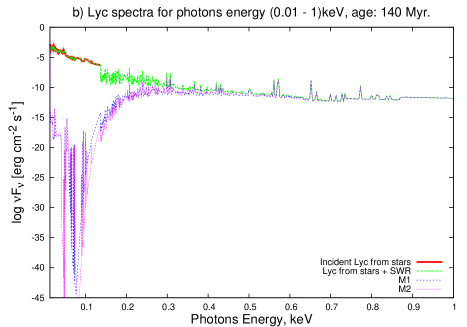
Figure 14: Changes of the Lyc-spectrum from the stars during the transfer of ionizing radiation through the DG. The upper panel refers to the energy range between 13 and 140 eV. The lower panel extends up to 1 keV. All fluxes are given at a distance of 2.3 kpc from the center of galaxy (at the outer edge of the modelling volume).

It must be also once again remarked that in our models we calculated the diffuse component of the the ionizing radiation in outward only approximation. Probably, the diffuse ionizing radiation does not play a crucial role in the formation of the global structure of diffuse ionized gas. Nevertheless, as we have shown above, important emission lines can be partly formed in low-ionization zones of small spatial scale. Existing 3D codes (such as Mocassin; Ercolano et al., 2003) can calculate the diffuse ionizing field in regions shadowed by TDS, but they need a very large amount of computing time. Moreover, Mocassin is based on the statistical analysis of random propagation of photon packages. We think that for the problem at hand a deterministic approach, based on the detailed calculation of diffuse radiation propagation, is more useful. Therefore, we are developing an extension of the MPhM, able to follow in detail the diffuse ionizing radiation field (i.e. we will relax the outward-only approximation). Such method can be very useful for the correct investigation of the ionization structure in the shadow regions beyond the TDS. As mentioned above, this method can also help simulate the leakage of ionizing photons from a galaxy in a more realistic way.

7 Discussion

In this paper we have described a way to combine detailed ChDS of DGs with a state-of-the-art MPhM, to study the emission properties of star-forming galaxies and compare them with observations.

We have performed two types of analysis of the obtained MPhM results: $(i)$ model predictions and $(ii)$ consistency checks. Important emission line ratios have been calculated and compared with observations of a DG galaxy with structural parameters similar to the simulated one (see Sect. 5.3). The calculated escape fraction of ionizing photons $f_{esc}$ is calculated, too, and compared with results of radiative transfer hydrodynamical simulations (Sect. 6). The results of these calculations are briefly summarized and discussed in Sect. 7.1. With consistency checks we mean instead tests in which some galactic properties are known because of the results of the ChDSs. The same galactic properties are re-derived as an observer would do, based on the MPhM results. The analysis of the oxygen abundances (Sect. 5.4) and of the empirical determinations of the SFR in galaxies (Sect. 5.5) belong to this category. The results of these two tests are briefly discussed below (Sect. 7.2). We shall not forget that our analysis is based on some simplifying hypotheses and there are potentially important physical processes (e.g. the dust reprocessing) that have not been considered. We will briefly discuss these limitations in Sect. 7.3. Finally, some overall conclusions are drawn in Sect. 8.

7.1 Model predictions

We have calculated the intensities of observationally relevant emission lines both integrating along angular sectors (Sect. 4.2) and across apertures (Sect. 5.2). Some line intensities and intensity ratios, such as [OIII]$\lambda 5007$/H$\beta$ and H$\alpha$/H$\beta$, nicely fit into the range of observed intensity ratios (see Table 2) whereas some others do not.

In particular, calculated [OII] line intensities are very weak. It should be also remarked here that the average final oxygen abundance of the model L8F is 12+log(O/H)=7.84 (see RH13). We have also calculated model M1 at a higher metallicity, corresponding to the oxygen abundance 12+$\log$O/H=8.2. For such model, the calculated [OII] line intensities are still weak in comparison with observations. This is due to the fact that the supershell created by the stellar feedback in ChDSs is not dense enough to block O-ionizing photons. O⁺ is thus very scarce (see Fig. 10) and this clearly implies very few O⁺ transitions. The inclusion of artificial density enhancements close to the supershell (model M2) helps creating a shell of singly ionized oxygen. For model M2, thus, also intensity ratios such as [OII]$\lambda 3727$/$H\beta$ are in agreement with observations.

We will provide a comprehensive study on the models like M1 and M2 at different metallicities in a future paper.

We have also calculated, for each angular sector, the escape fraction of ionizing photons $f_{esc}$. This fraction is generally very high along directions close to the symmetry axis, i.e. towards the poles, because the superbubble propagates preferentially along these directions due to the very steep pressure gradients. The global $f_{esc}$ ranges from $\sim$ 0.3 to $\sim$ 0.6, with an average of about 0.4. Results of radiative hydrodynamical simulations of DGs generally show lower values of $f_{esc}$, although the results crucially depend on the details of the feedback scheme and on the adopted star formation efficiencies (see e.g. Fujita et al., 2003). Escape fractions calculated for model M2 are instead generally low. They can be of the order of 0.3–0.5 only along directions close to the symmetry axis and only for a limited amount of time, otherwise their values are of the order of 0.01. With such low values of $f_{esc}$ one can not expect that DGs significantly contribute to the reionization of the universe as concluded by Vanzella et al. (2012). In M2 models it was assumed that the TDS has the same density in all sectors. Of course this is a just a first-order approximation. TDS in different sectors would be characterized by different density values; in some sectors TDS might be even absent. Therefore, in reality, the Lyc photon escape should be higher in the vertical direction. Thus, evidently, more accurate calculations are necessary to address more in detail the issue of the escape fraction (see also Sect. 7.3).

7.2 Consistency checks

The employed ChDSs follow in detail the evolution in space and time of important chemical elements, in particular oxygen. Based on the chemical composition of different regions of the galaxy, the MPhM calculates intensity ratios, as extensively described in the previous sections. On the other hand, these intensity ratios can be measured in real galaxies and are the principal way observers can infer the chemical composition of galaxies. We study the results of our simulations as an observer would do and derive the oxygen abundances based on calculated intensity ratios. As explained above, we use the $T_{e}$ and $R_{23}$ diagnostic methods.

In an ideal world, the abundances derived by means of intensity ratios should match the ’real’ ones, i.e. here the ones obtained from the ChDSs. This turns out to be the case only for some apertures and for some intervals of time (see Table 3). For other apertures and/or other intervals of time, the differences are significant. These disagreements are due to two reasons: $(i)$ the distribution of oxygen is very inhomogeneous and these inhomogeneities cannot be properly addressed by the applied diagnostic methods. These diagnostic methods work well in relatively uniform regions, but fail in the presence of very inhomogeneously distributed chemical elements. $(ii)$ Diagnostic methods commonly assume that most of the oxygen is either singly or/and doubly ionized. This is not the case in model M1, as we have shown in Fig. 10. For this reason, the adoption of unresolved density enhancements in thin shells (model M2) helps in obtaining ’observed’ ionization stages of oxygen close to the ’real’ ones.

In spite of that, our results indicate that the diagnostic methods should be used with a ’pinch of salt’ to say the less. For galaxies in which integral field spectroscopy is available, the difficulties of the diagnostic methods are reduced, as every chunk of the galaxy encloses a different abundance but the small-scale abundance inhomogeneities affect the integrated spectral lines much less. Notice also that Leroy et al. (2012) report of 1 kpc-scale variations and uncertainties of observed SFR indicators that are inherently e.g. caused by age effects and by intrinsic scatters of the indicators.

The H$\alpha$ emission from galaxies is extensively applied to derive their SFRs locally and globally (see Kennicutt, 1998, and references therein), because it is in fact assumed to be the signpost of (short-living) massive stars. For an assumed IMF the number of massive stars is, therefore, correlated with the SFR. As we have shown (Fig. 12) the total H$\alpha$ emission is up to $\sim$ 60% larger than the one expect from the stellar ionizing flux of our model. If one takes into account that, in addition, ionizing photons are also lost by the leakage from the galaxy after a few tens of Myr (Fig. 13) and that the H$\alpha$ -SFR relation by Calzetti et al. (2007) implies an even lower proportionality constant between SFR and H$\alpha$ luminosity, one can conclude that the additional ionization by cooling photons from the warm-hot gas is almost equal to the stellar contribution. At later times, the H$\alpha$ emission reduces, partly, due to the increasing amount of leaking ionizing photons. In this phase, an H$\alpha$ -based determination of the SFR would underestimate the real galactic SFR (see again Fig. 12). However, given the uncertainties associated to this SFR indicator, a factor of two agreement can be considered as fair.

Actually, it has been already reported in the literature that H$\alpha$ could be a poor SFR indicator in DGs. In particular, it has been noticed that the H$\alpha$ -based SFR estimates differ from the SFR estimates based on the UV emission at SFRs smaller that $\sim$ 0.01 M_⊙ yr^-1 and the discrepancy can be larger than a factor of 10 at SFR=10^-4 M_⊙ yr^-1 (Lee et al., 2009). This discrepancy has been associated to a top-light IMF in DGs with very mild SFRs (Pflamm-Altenburg, 2009). In such galaxies, there is some star formation but not enough generation of the very massive stars able to produce H$\alpha$ emission. Notice, however, that our SFR (nominally 2.67 $\cdot$ 10^-2 M_⊙ yr^-1) is not extremely low. In this SFR range the effect of the top-light IMF should not be very significant. Notice also that the leakage of H$\alpha$ photons can be significant for our model and it is surely even more significant for galaxies with lower masses, where galactic winds are more prominent (see RH13). It is thus reasonable to assume that the discrepancy between H$\alpha$ -based and UV-based SFRs noticed by Lee et al. (2009) also depends on $f_{esc}$. Notice however also that, as Leroy et al. (2012) point out, Starburst99 simulations of an evolving single stellar population imply an intrinsic scatter of almost 0.3 dex in H$\alpha$ -based SFR estimates and about 0.5 dex in FUV-based determinations. We will add these issues in detail in a follow-up paper.

7.3 Model limitations

We have already outlined three limitations of the study presented in this paper, namely:

• The MPhM is applied in a post-processing step, thus the energy due to radiative processes does not feed back on the gas and does not affect the hydrodynamics.

• The gas densities, obtained from the ChDSs, are always below a few particles per cm³, i.e. they never reach the peak densities of typical HII regions.

• The MPhM calculations are based on the outward-only approximation (the only one available with CLOUDY)

We do not plan to relax the first simplification because this would require computationally expensive radiative hydrodynamics simulations. These calculations do not allow to explore a wide parameter space and, moreover, simplifying assumptions about the radiation field and the propagation of radiation need to be made. Notwithstanding the limitations, we think that our approach is reasonable because it is computationally inexpensive and the radiation transfer equations can be calculated with great accuracy. We do plan to relax the last two simplifications though.

The second limitation can be relaxed by using a multi-phase ISM treatment, that takes into account (in the same computational cell) a warm-hot, diluted phase, and a colder, denser phase, that can reach the peak densities of typical HII regions and more. Notice also that, for the galaxy NGC1569, Westmoquette et al. (2007, 2008) concluded from H$\alpha$ line decompositions that the light profile is composed of a bright, narrow feature originating within a narrow region of $\sim$700$\times$500 pc in size, roughly centred on the bright super star cluster A, and of an underlying broad component emerging from turbulent mixing layers on the surfaces the clouds which are embedded into the hot, fast-flowing winds from the young star clusters and experience evaporation and/or ablation of material. A new 3D chemo-dynamical code (cdFLASH) is already available (Mitchell et al., in preparation) and needs to be applied to the problem at hand.

The last limitation (the outward-only approximation) will be relaxed once a new CLOUDY wrapper (currently under development) will be available.

It is, however, worth mentioning that the model presented here lacks another potentially relevant ingredient: dust. Dust can increase the opacities of many lines along all directions, thus affecting our results significantly. The reason why dust has not been included so far is not technical: the MPhM wrapper and the underlying CLOUDY code can already treat dust. We have decided to neglect dust only for the purpose of clarity and in order to avoid cluttering of the (already long) text. We have however already performed a pilot study with dust. Assuming a gas-to-dust ratio of 1400 (ten times larger than the Milky Way value, typical for DGs) we find very little differences between the results of a dusty model and the ones presented in this paper. However, for smaller gas-to-dust ratios the effect of dust can be very significant. We will explore the dust effect in a short follow-up paper.

8 Conclusions

The main conclusions of the present study can be summarized as follows:

• Our combined ChDS-MPhM approach is able to produce intensity ratios of important emission lines which are in agreement with the observations. This is not the case for O⁺ lines, which are severely underestimated. The reason is that the densities are on average low and most of oxygen in the model galaxy is in high ionization stages.

• An artificial density enhancement (simulating an unresolved thin shell) brings also [OII] lines in agreement with observations.

• We obtain typical escape fractions of ionizing photons ($f_{esc}$) of the order of 40%. This escape fraction reduces to a few per cent if we consider the same density enhancements described above.

• Diagnostic methods ($T_{e}$ and $R_{23}$) are generally not able to reproduce the real abundance of heavy elements, obtained by means of the chemo-dynamical simulations. This is due in part to the inherent limitations in the diagnostic methods, in part to the fact that in our simulation very little oxygen is neutral or singly ionized.

• We have shown that the Kennicutt’s estimate of the SFR in galaxies based on the H$\alpha$ emission is inaccurate. Part of the inaccuracy is due to the significant contribution of the warm-hot gas to the H$\alpha$ emission. Part is instead due to the fact that the leakage of ionizing photons out of a typical starbursting galaxy can be significant and that naturally affects the global H$\alpha$ emission.

References

- Angeretti et al. (2005) Angeretti, L., Tosi, M., Greggio, L., et al. 2005, AJ, 129, 2203
- Baldwin et al. (1981) Baldwin, J. A., Philips, M. M., & Terlevich, R. 1981, PASP, 93, 5
- Buhajenko & Melekh (2013) Buhajenko, O., & Melekh, B.Ya. 2013, 20th Open Young Scientist’s Conference on Astronomy and Space Physics. Abstracts. April 22-27, 2013, Kyiv, 56.
- Calzetti et al. (2007) Calzetti, D., Kennicutt, R.C., Engelbracht, C.W., et al. 2012, ApJ, 666, 870
- Compostella et al. (2013) Compostella, M., Cantalupo, S., & Porciani, C. 2013, MNRAS, 435, 3169
- Dopita & Sutherland (2003) Dopita, M. A., & Sutherland, R. S. 2003, Astrophysics of the diffuse universe, Berlin, New York: Springer, 2003. Astronomy and astrophysics library, ISBN 3540433627
- Draine (2011) Draine, B.T., Physics of the Interstellar and Intergalactic Medium (Princeton University Press, 2011), 560 p.
- Ercolano et al. (2003) Ercolano B., Barlow M. J., Storey P. J., & Liu X.-W. 2003, MNRAS, 340, 1136.
-
Ferland (2008)
Ferland, G.J., Hazy, a Brief Introduction
to Cloudy (University of Kentucky, Physics Department Internal
Report, 2008), 807 p.
http://www.nublado.org, http://viewvc.nublado.org/index.cgi/
tags/release/c08.00/docs/?root=cloudy - Freyer et al. (2003) Freyer, T., Hensler, G., & Yorke, H. W. 2003, ApJ 594, 888
- Fujita et al. (2003) Fujita, A, Martin, C. L., Mac Low, M.-M., Abel, T. 2003, ApJ, 599, 50
- Garnett (1992) Garnett, D. R. 1992, AJ, 103, 1330.
- Hirano et al. (2014) Hirano, S., Hosokawa, T., Yoshida, N., et al. 2014, ApJ, 781, 60
- Golovaty et al. (1993) Golovaty, V. V., Dmiterko, V.I., Mal’kov, Yu. F., & Rokach, O. V. 1993, Astronomical Report, 37, 346
- Johnson et al. (2012) Johnson, M., Hunter, D. A., Oh, S.-H., et al. 2012, AJ, 144, 152
- Kehrig et al. (2004) Kehrig, C., Telles, E., Cuisinier, F. 2004, AJ, 128, 1141.
- Kennicutt (1998) Kennicutt, R. C., Jr. 1998, ApJ, 498, 541
- Kimm & Cen (2014) Kimm, T., & Cen, R. 2014, ApJ, 788, 121
- Kobulnicky & Skillman (1997) Kobulnicky, H. A., & Skillman, E. D. 1997, ApJ, 489, 636 (KS97)
- Koshmak & Melekh (2013) Koshmak, I. O., & Melekh, B. Ya. 2013, Kinematics and Physics of Celestial Bodies, 29, 257.
- Koshmak & Melekh (2014) Koshmak, I. O., & Melekh, B. Ya. 2014, Kinematics and Physics of Celestial Bodies, 30, 70.
- Krumholz et al. (2012) Krumholz, M. R., Klein, R. I., & McKee, C. F. 2012, ApJ, 754, 71
- Lee et al. (2009) Lee, J. C., Gil de Paz, A., Tremonti, C., et al. 2009, ApJ, 706, 599.
- Leitherer et al. (1999) Leitherer, C., Schaerer, D., Goldader, J. D.,et al. 1999 ApJS, 123, 3.
- Leroy et al. (2012) Leroy, A.K., Bigiel, F., de Blok, W.J.G., et al. 2012, Astron. J., 144, 3
- Mathis et al. (1998) Mathis, J. M., Torres-Peimbert, S, & Peimbert, M. 1998, ApJ, 495, 328.
- McCaugh (1991) McCaugh, S. S. 1991, ApJ, 380, 140.
- Melekh (2006) Melekh, B. Ya. 2006, Journal of Physical Studies, 10, 148.
- Melekh (2007) Melekh, B. Ya. 2007, Journal of Physical Studies, 11, 353.
- Morisset (2006) Morisset, C. 2006, Planetary Nebulae in our Galaxy and Beyond. Proceedings IAU Symposium, 234, 467.
- Osterbrock & Ferland (2005) Osterbrock, D. E., & Ferland, G. J. 2005, Astrophysics of Gaseous Nebulae and Active Galactic Nuclei. Second Edition, Saulito, California: University Science Book, ISBN 1-891389-34-3
- Paardekooper et al. (2013) Paardekooper, J.-P., Khochfar, S., & Dalla Vecchia, C. 2013, MNRAS, 429, L94
- Pagel et al. (1979) Pagel, B. E. J., Edmunds, M. G., Blackwell, D. E., Chun, M. S., & Smith, G. 1979, MNRAS, 189, 95
- Pagel et al. (1992) Pagel, B. E. J., Simonson, E. A., Terlevich, R. J., & Edmunds, M. G. 1992, MNRAS, 255, 325
- Peimbert (1967) Peimbert, M. 1967, ApJ, 150, 825
- Pettini & Pagel (2004) Pettini, M., & Pagel, B. E. J. 2004, MNRAS, 348, L59
- Pflamm-Altenburg (2009) Pflamm-Altenburg, J., Weidner, C., & Kroupa, P. 2009, MNRAS, 395, 394
- Pilyugin (2003) Pilyugin, L. S. 2003, A&A, 399, 1003
- Press et al. (1992) Press W. H., Teukolsky S. A., Vetterling W. T., Flannery B. P., Numerical Recipes in C, The Art of Scientific Computing: Second Edition (Cambrige University Press, 1992), 980 p.
- Recchi & Hensler (2013) Recchi, S., & Hensler, G. 2013, A&A, 551, A41
- Recchi et al. (2006) Recchi, S., Hensler, G., Angeretti, L., & Matteucci, F. 2006, A&A, 445, 875
- Recchi et al. (2001) Recchi, S., Matteucci, F., & D’Ercole, A. 2001, MNRAS, 322, 800
- Recchi et al. (2004) Recchi, S., Matteucci, F., D’Ercole, A., & Tosi, M. 2004, A&A, 426, 37
- Relano et al. (2012) Relano, M., Kennicutt, R. C., Jr., Eldridge, J. J., Lee, J. C., & Verley, S. 2012, MNRAS, 423, 2933
- Searle (1971) Searle, L. 1971, ApJ, 168, 327
- Shaw (1995) Shaw, R. A., & Dufour, R. J. 1995, PASP, 107, 896
- Stasińska (2002) Stasińska, G. 2002, RevMexAA, 12, 62
- Stasińska (2006) Stasińska, G. 2006, A&A, 454, L127
- Tassoul (1978) Tassoul, J.-L. 1978, Theory of rotating stars, Princeton Series in Astrophysics, Princeton: University Press
- Tsamis & Péquignot (2005) Tsamis, Y. G., & Péquignot, D. 2005, MNRAS, 364, 687
- Vanzella et al. (2012) Vanzella, E., Nonino, M., Cristiani, S., et al. 2012, MNRAS, 424, L54
- Walter et al. (2007) Walter, F., Cannon, J. M., Roussel, H., et al. 2007, ApJ, 661, 102
- Westmoquette et al. (2007) Westmoquette, M.S., Exter, K.M., Smith, L.J., & Gallagher, J.S.III 2007, MNRAS, 381, 894
- Westmoquette et al. (2008) Westmoquette, M.S., Smith, L.J., & Gallagher, J.S.III 2008, MNRAS, 383, 864
- Wise et al. (2014) Wise, J. H., Demchenko, V. G., Halicek, M. T., et al. 2014, MNRAS, 442, 2560
- Yajima et al. (2011) Yajima, H., Choi, J.-H., & Nagamine, K. 2011, MNRAS, 412, 411
- Yoshida et al. (2007) Yoshida, N., Oh, S. P., Kitayama, T., & Hernquist, L. 2007, ApJ, 663, 687