Microscopic theory and quantum simulation of atomic heat transport

Abstract

Quantum simulation methods based on density-functional theory are currently deemed unfit to cope with atomic heat transport within the Green-Kubo formalism, because quantum-mechanical energy densities and currents are inherently ill-defined at the atomic scale. We show that, while this difficulty would also affect classical simulations, thermal conductivity is indeed insensitive to such ill-definedness by virtue of a sort of gauge invariance resulting from energy extensivity and conservation. Based on these findings, we derive an expression for the adiabatic energy flux from density-functional theory, which allows heat transport to be simulated using ab-initio equilibrium molecular dynamics. Our methodology is demonstrated by comparing its predictions with those of classical equilibrium and ab-initio non-equilibrium (Müller-Plathe) simulations for a liquid-Argon model, and finally applied to heavy water at ambient conditions.

Introduction

Understanding heat transport is key in many fields of science and technology, such as materials and planetary sciences, energy saving, heat dissipation and shielding, or thermoelectric conversion, to name but a few. Heat transport in insulators is determined by the dynamics of atoms, the electrons following adiabatically in their ground state. Simulating atomic heat transport usually relies on Boltzmann’s kinetic approach Klemens:1959 , or on molecular dynamics (MD), both in its equilibrium (Green-Kubo, GK Green:1954 ; Kubo ; Evans-Morriss ; Allen-Tildesley ) and non-equilibrium Evans-Morriss ; Allen-Tildesley ; Mueller-Plathe:1997 flavors. The Boltzmann equation only applies to crystalline solids well below melting, whereas classical MD (CMD) bears on those materials and conditions that can be modeled by inter-atomic potentials. Equilibrium ab-initio (AI) MD Car:1985 ; Marx-Hutter is set to overcome these limitations, but it is still surprisingly thought to be unfit to cope with thermal transport because in first-principles calculations it is impossible to uniquely decompose the total energy into individual contributions from each atom (excerpted from Ref. Stackhouse:2010, ). Such a unique decomposition is not possible in classical mechanics either, because the potential energy of a system of interacting atoms can be partitioned into local contributions in an infinite number of equivalent ways. The quantum mechanical energy density is also affected by a similar indeterminacy. Notwithstanding, the expression for the heat conductivity derived from any sensible energy partitioning or density should obviously be well defined, as any measurable quantity must.

In this work we first demonstrate that the thermal conductivity resulting from the GK relation is unaffected by the indeterminacy of the microscopic energy density; we then introduce a form of energy density, and a corresponding adiabatic energy flux, from which heat transport coefficients can be computed within the GK formalism, using density-functional theory (DFT). Our approach is validated by comparing the results of equilibrium AIMD with those of non-equilibrium (Müller-Plathe, MP Mueller-Plathe:1997 ) AIMD and equilibrium CMD simulations for a liquid-Argon model, for which accurate inter-atomic potentials are derived by matching the forces generated by them with quantum-mechanical forces computed along the AIMD trajectories. The case of molecular fluids is finally addressed, and illustrated in the case of water at ambient conditions.

Theory

According to the GK theory Green:1954 ; Kubo , the atomic thermal conductivity of an isotropic system is given by:

$$\kappa=\frac{1}{3Vk_{B}T^{2}}\int_{0}^{\infty}\langle\mathbf{J}_{q}(t)\cdot\mathbf{J}_{q}(0)\rangle dt,$$ (1)

where brackets $\langle\cdot\rangle$ indicate canonical averages, $k_{B}$ is the Boltzmann constant, $V$ and $T$ the system volume and temperature, $\mathbf{J}_{q}(t)=\int\bigl{(}\mathbf{j}_{e}(\mathbf{r},t)+\left(p+\langle e\rangle\right)\mathbf{v}(\mathbf{r},t)\bigr{)}d\mathbf{r}$ is the macroscopic heat flux, $\mathbf{j}_{e}$, $\mathbf{v}$, $p$, and $\langle e\rangle$ being the energy-current density, local velocity field, and equilibrium values of pressure and energy density, respectively Kadanoff-Martin ; Forster . For further reference, we define as diffusive a flux that results in a non-vanishing GK conductivity, according to Eq. (1). The integral of the velocity field is non diffusive in solids and can be assumed to vanish in one-component fluids, because of momentum conservation. In these cases, as well as in molecular fluids as we will see, we can therefore assume that heat and energy fluxes coincide.

Energy is extensive: it can thus be expressed as the integral of a density, which is defined up to the divergence of a bounded vector field: two densities that differ by such a divergence, $e(\mathbf{r})$ and $e^{\prime}(\mathbf{r})=e(\mathbf{r})+\partial\cdot\mathbf{p}(\mathbf{r})$, are indeed equivalent, in that their integrals differ by a surface term, which is irrelevant in the thermodinamic limit, and can thus be thought of as different gauges of a same scalar field. Energy is also conserved: therefore, for any given gauge of its density, $e$, a corresponding current density, $\mathbf{j}_{e}$, can be defined so as to satisfy the continuity equation:

$$\dot{e}(\mathbf{r},t)+\partial\cdot\mathbf{j}_{e}(\mathbf{r},t)=0.$$ (2)

According to Eq. (2) the macroscopic fluxes in two different energy gauges differ by a total time derivative, which is non-diffusive: $\mathbf{J}^{\prime}_{e}(t)=\mathbf{J}_{e}(t)+\dot{\mathbf{P}}(t)$, where $\mathbf{P}(t)=\int\mathbf{p}(\mathbf{r},t)d\mathbf{r}$. The equality of the corresponding heat conductivities results from the following

Lemma—Let $\mathbf{J}_{1}$ and $\mathbf{J}_{2}$ be two macroscopic fluxes defined for a same system, and $\mathbf{J}_{12}=\mathbf{J}_{1}+\mathbf{J}_{2}$ their sum. The corresponding GK conductivities, $\kappa_{1}$, $\kappa_{2}$, and $\kappa_{12}$ satisfy the relation: $\left|\kappa_{12}-\kappa_{1}-\kappa_{2}\right|\leq 2\sqrt{\kappa_{1}\kappa_{2}}$.

Proof—Let the energy displacement associated with the flux $\mathbf{J}_{i}$ be defined as: $\mathbf{D}_{i}(t)=\frac{1}{\sqrt{6Vk_{B}T^{2}}}\int_{0}^{t}\mathbf{J}_{i}(t^{\prime})dt^{\prime}$. The standard Einstein relation Helfand:1960 states that: $\kappa_{i}=\lim_{t\to\infty}\left\langle|\mathbf{D}_{i}(t)|^{2}\right\rangle/t$; it follows that: $\kappa_{12}=\kappa_{1}+\kappa_{2}+\lim_{t\to\infty}2\left\langle\mathbf{D}_{1}(t)\cdot\mathbf{D}_{2}(t)\right\rangle/t$. Canonical averages of products of phase-space functions can be seen as scalar products: the lemma then follows from the Cauchy-Schwartz inequality, as applied to the last relation. ∎

The application of the GK methodology to multi-component fluids requires some generalizations because the presence of multiple atomic species and the existence of additional hydrodynamical modes (one conserved number per atomic species) do not permit to identify the velocity field with the mass-current density, its integral with the total momentum, and the heat flux with the energy flux. In molecular fluids, however, this identification can still be done because the integral of the velocity field, while not a constant, is a non-diffusive flux, thus not contributing to the heat conductivity. In order to demonstrate this statement, we first define the fluxes $\mathbf{J}_{AB}=n_{B}\mbox{{V}}_{A}-n_{A}\mathbf{V}_{B}$, where $A$ and $B$ indicate any two atomic species, $n_{A}/n_{B}$ their stoichiometric ratio, and $\mathbf{V}_{S}=\sum_{i\in S}\mathbf{v}_{i}$ is the sum of the velocities of all the atoms of a same species $S$. The integral $\int_{0}^{t}\mathbf{J}_{AB}(t^{\prime})dt^{\prime}$ is equal to the sum of the variations of all the $AB$ relative positions in a same molecule, which is bound by the sum of the variations of all the $AB$ distances. $\mathbf{J}_{AB}$ is therefore a non-diffusive flux. We have $N(N-1)/2$ such non-diffusive fluxes, $N$ being the number of species, of which only $N-1$ are linearly independent; furthermore the flux $J_{M}=\sum_{S}M_{S}\mathbf{V}_{S}$ ($M_{S}$ is the mass of the $S$-th atomic species) is the total momentum, and is thus non-diffusive. We have therefore $N$ independent linear combinations of the $\mathbf{V}_{S}$ fluxes that are non-diffusive. We conclude that all of them, as well as their sum, $\mathbf{V}(t)=\sum_{S}\mathbf{V}_{S}(t)=\frac{1}{V}\int\mathbf{v}(\mathbf{r},t)d\mathbf{r}$, are also non-diffusive.

In order to derive an expression for the macroscopic energy flux appearing in the GK formula, Eq. (1), we first multiply the continuity equation, Eq. (2), by $\mathbf{r}$ and integrate by parts, to obtain the first moment of the time derivative of the energy density:

$$\mathbf{J}_{e}(t)=\int\dot{e}(\mathbf{r},t)\mathbf{r}d\mathbf{r}.$$ (3)

In periodic boundary conditions (PBC) Eq. (3) is ill-defined for the very same reason why macroscopic polarization in dielectrics is so Resta-Vanderbilt:2007 . In CMD the usual expression for the energy flux in terms of atomic energies and forces Allen-Tildesley is recovered from Eq. (3) by the somewhat arbitrary definition: $e(\mathbf{r},t)=\sum_{I}e_{I}(\mathbf{R},\mathbf{V})\delta(\mathbf{r}-\mathbf{R}_{I})$, where $e_{I}=\frac{1}{2}M_{I}V_{I}^{2}+\frac{1}{2}\sum_{J\neq I}v(|\mathbf{R}_{J}-\mathbf{R}_{I}|)$, $\mathbf{R}=\{\mathbf{R}_{I}\}$, and $\mathbf{V}=\{\mathbf{V}_{I}\}$ are the atomic energies, positions, and velocities, and by reducing the resulting expression to a boundary-insensitive form. In DFT an energy density can be defined, which is however inherently ill-determined because of the non-uniqueness of the quantum-mechanical kinetic and classical electrostatic energy densities Chetty:1992 ; Ramprasad:2002 . Our previous analysis demonstrates that, in spite of previous worries to the contrary, the transport coefficients derived from a DFT energy density through the GK formula, Eq. (1), are well defined, provided a macroscopic energy flux can be computed from Eq. (3) in PBC. To this end, among many equivalent gauges, we choose to represent the DFT total energy as the integral of the density:

$$e_{DFT}(\mathbf{r})=\sum_{I}\delta(\mathbf{r}-\mathbf{R}_{I})e^{0}_{I}+\mathrm{Re}\sum_{v}\varphi_{v}^{*}(\mathbf{r})\bigl{(}\hat{H}_{KS}\varphi_{v}(\mathbf{r})\bigr{)}-\frac{1}{2}\rho(\mathbf{r})v_{H}(\mathbf{r})+\left(\epsilon_{XC}(\mathbf{r})-v_{XC}(\mathbf{r})\right)\rho(\mathbf{r}),$$ (4)

where $e^{0}_{I}=\frac{1}{2}M_{I}V_{I}^{2}+w_{I}$ are bare ionic energies; $M_{I}$, $Z_{I}$, and $w_{I}=\frac{1}{2}\sum_{J\neq I}\frac{Z_{I}Z_{J}}{|\mathbf{R}_{I}-\mathbf{R}_{J}|}$ being ionic masses, charges, and electrostatic energies, respectively; the electron charge is assumed to be one; $\hat{H}_{KS}$ is the instantaneous Kohn-Sham (KS) Hamiltonian, $\varphi_{v}$’s its occupied eigenfunctions, and $\rho(\mathbf{r})=\sum_{v}|\varphi_{v}(\mathbf{r})|^{2}$ the ground-state electron-density distribution; $v_{H}$ and $v_{XC}$ are Hartree and exchange-correlation (XC) potentials, and $\epsilon_{XC}$ is a local XC energy per particle, defined by the relation: $E_{XC}=\int\epsilon_{XC}[\rho](\mathbf{r})\rho(\mathbf{r})d\mathbf{r}$. The energy density of Eq. (4) depends on time through atomic positions and velocities and KS orbitals. Inserting its time derivative into Eq. (3) and using the Born-Oppenheimer (BO) equations of motion for the nuclei ($M_{I}\mathbf{\dot{V}}_{I}=-\partial E_{DFT}/\partial\mathbf{R}_{I}$), the resulting adiabatic energy flux can be expressed as:

$$\mathbf{J}_{\epsilon}=\mathbf{J}_{KS}+\mathbf{J}_{H}+\mathbf{J}^{\prime}_{0}+\mathbf{J}_{0}+\mathbf{J}_{XC}.$$ (5)

The five fluxes in Eq. (5) are defined as:

$$\mathbf{J}_{KS} =\sum_{v}\left(\langle\varphi_{v}|\mathbf{r}\hat{H}_{KS}|\dot{\varphi}_{v}\rangle+\varepsilon_{v}\langle\dot{\varphi}_{v}|\mathbf{r}|\varphi_{v}\rangle\right),$$ (6)

$$\mathbf{J}_{H} =\frac{1}{4\pi}\int\dot{v}_{H}(\mathbf{r})\nabla v_{H}(\mathbf{r})d\mathbf{r},$$ (7)

$$\mathbf{J}^{\prime}_{0} =\sum_{v,I}\left\langle\varphi_{v}\left|(\mathbf{r}-\mathbf{R}_{I})\left(\mathbf{V}_{I}\cdot\nabla_{I}\hat{v}_{0}\right)\right|\varphi_{v}\right\rangle,$$ (8)

$$\mathbf{J}_{0} =\sum_{I}\Bigl{[}\mathbf{V}_{I}e^{0}_{I}+\sum_{L\neq I}(\mathbf{R}_{I}-\mathbf{R}_{L})\left(\mathbf{V}_{L}\cdot\nabla_{L}w_{I}\right)\Bigr{]},$$ (9)

$$\mathbf{J}_{XC} =\begin{cases}0&\text{(LDA)}\\ -\int\rho(\mathbf{r})\dot{\rho}(\mathbf{r})\partial\epsilon_{GGA}(\mathbf{r})d\mathbf{r}&\text{(GGA)},\end{cases}$$ (10)

where $\varepsilon_{v}$ in Eq. (6) is the $v$-th eigenvalue of the KS Hamiltonian; $\nabla=\frac{\partial}{\partial\mathbf{r}}$ and $\nabla_{I}=\frac{\partial}{\partial\mathbf{R}_{I}}$ in Eqs. (7-9) indicate the gradients with respect to the argument of the function and to the $I$-th atomic position, respectively; the simbol $\hat{v}_{0}$ in Eq. (8) indicates the (possibly non-local) ionic (pseudo-) potential acting on the electrons; finally, “LDA” and “GGA” in Eq. (10) indicate the local-density KS:1965 and generalized-gradient Perdew:1996 approximations to the XC energy functional, respectively, and $\partial\epsilon_{GGA}$ the derivative of the GGA XC local energy per particle with respect to density gradients. Eq. (5) can be derived from Eqs. (3-4) with some tedious but straightforward algebra (see Methods). The last four terms on its right-hand side, Eqs. (7–10), are manifestly boundary-insensitive, whilst the first, Eq. (6), is not, because the position operator appearing therein is ill-defined in PBC. Within the adiabatic time evolution that is assumed in AIMD, however, the time derivative of a KS orbital, as well as its product with the KS Hamiltonian, are orthogonal to the orbital itself in the “parallel transport” gauge where KS orbitals are real Thouless:1983 ; Resta:2000 : $\langle\varphi_{v}|\dot{\varphi}_{v}\rangle=0$ and $\langle\varphi_{v}|H_{KS}|\dot{\varphi}_{v}\rangle=0.$ Therefore, in order to evaluate Eq. (6), one only needs the projection of $\mathbf{r}|\varphi_{v}\rangle$ onto the manifold orthogonal to $\varphi_{v}$, which is well defined in PBC. Actually, by expanding $\dot{\varphi}_{v}$ in the basis of the eigenstates of the instantaneous KS Hamiltonian Thouless:1983 , one sees that only the projection of $\mathbf{r}|\varphi_{v}\rangle$ onto the empty-state manifold, $|\bar{\varphi}_{v}^{\alpha}\rangle=\hat{P}_{c}x^{\alpha}|\varphi_{v}\rangle,$ contributes to $\mathbf{J}_{KS}$, where $\hat{P}_{c}=1-\sum_{v}|\varphi_{v}\rangle\langle\varphi_{v}|$ and $x^{\alpha}$ is the $\alpha$-th Cartesian component of $\mathbf{r}$. Using the standard prescription adopted in density-functional perturbation theory (DFPT), such a projection can be computed by solving the linear equation Baroni:2001 :

$$(\hat{H}_{KS}-\varepsilon_{v})|\bar{\varphi}_{v}^{\alpha}\rangle=\hat{P}_{c}[\hat{H}_{KS},x^{\alpha}]|\varphi_{v}\rangle,$$ (11)

where the ill-definedness of the solution, due to the singularity of the left-hand side, is lifted by enforcing its orthogonality to the occupied-state manifold. In terms of the $\bar{\varphi}_{v}^{\alpha}$’s Eq. (6) reads:

$$J_{KS}^{\alpha}=\sum_{v}\left(\langle\bar{\varphi}_{v}^{\alpha}|H_{KS}|\dot{\varphi}_{v}\rangle+\varepsilon_{v}\langle\dot{\varphi}_{v}|\bar{\varphi}_{v}^{\alpha}\rangle\right).$$ (12)

The flux in Eq. (12) is not manifestly invariant with respect to the arbitrary choice of the zero of the one-electron energy levels. A shift of the energy zero by a quantity $\Delta\epsilon$ results in a shift of the Kohn-Sham energy flux: $J_{KS}^{\alpha}\rightarrow J_{KS}^{\alpha}+\Delta\varepsilon\sum_{v}\left(\langle\bar{\varphi}_{v}^{\alpha}|\dot{\varphi}_{v}\rangle+\langle\dot{\varphi}_{v}|\bar{\varphi}_{v}^{\alpha}\rangle\right)=J_{KS}^{\alpha}+\Delta\varepsilon J_{\rho}^{\alpha},$ where $\mathbf{J}_{\rho}$ is the adiabatic electronic macroscopic flux introduced in Ref. Thouless:1983 . The electronic current is the difference between the total charge current and its ionic component: the first is by definition non-diffusive in insulators, while the second is so in mono-atomic and molecular systems, as we have seen when discussing the latter. We conclude that the electronic flux is non-diffusive in insulators, thus not contributing to their heat conductivity and lifting the apparent indeterminacy of Eq. (12).

Numerical simulation

The methodology presented above has been implemented in the Quantum ESPRESSO suite of computer codes QE:2009 : a Car-Parrinello (CP) Car:1985 AIMD trajectory is first generated using the cp.x code; the energy flux is then evaluated along this trajectory according to Eqs. (5-9) by an add-on to the pw.x code implemented using several DFPT routines borrowed from the ph.x code; the thermal conductivity is finally computed from the GK relation, Eq. (1), or the equivalent Einstein relation Helfand:1960 .

In order to demonstrate this methodology, we compare its predictions with those from CMD LAMMPS:1995 for a system whose DFT BO energy surface can be accurately mimicked by pair potentials. Not aiming at a realistic description of any specific system, but rather at the ease and accuracy of the classical representation of the DFT BO surface, we choose liquid Argon and use the LDA XC functional, in spite of the well known inability of the latter to capture dispersion forces. This reference system will be dubbed “LDA-Ar”. KS orbitals are treated within the plane-wave (PW) pseudo-potential (PP) method PP . Our model consists of 108 atoms in a periodically repeated cubic supercell with an edge of 33 a.u., corresponding to a density of 1.34 $\mathrm{g/cm^{3}}.$ AIMD trajectories were generated via the Car-Parrinello dynamics Car:1985 for 100 picoseconds (ps), using a time step of 0.242 femtoseconds (fs) and a fictitious electronic mass of 1000 electronic masses, at two different temperatures, $\mathrm{T}=250$ and $400\thinspace\mathrm{K}$. The fictitious electronic temperature was monitored and checked not to be subject to any significant drift. The BO energy surface was modeled with a sum of classical pair potentials of the form $V(r)=P_{2}(r)\mathrm{e}^{-\alpha r}$, where $P_{2}$ is a second-order polynomial, whose parameters were determined independently for each temperature by a least-square fit of the classical vs. quantum-mechanical forces computed along the AIMD trajectory. Self-diffusion coefficients of $(10.8\pm 0.1)$, and $(15.6\pm 0.2)\times 10^{-5}\mathrm{cm^{2}/s}$ were estimated along the two AIMD trajectories, in close agreement with the CMD values $(10.3\pm 0.1)$, and $(15.8\pm 0.2)\times 10^{-5}\mathrm{cm^{2}/s}$, thus confirming the quality of the classical model. Radial distribution functions computed from AIMD and CMD trajectories were also found to be very similar.

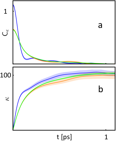
Figure 1: Time correlations of the energy flux in LDA Ar. (a) $C_{e}(t)=\frac{1}{3Vk_{B}T^{2}}\langle\mathbf{J}_{e}(t)\cdot\mathbf{J}_{e}(0)\rangle\thinspace\mathrm{[10^{15}mWK^{-1}s^{-1}]}$. (b) $\kappa(t)=\int_{0}^{t}C_{e}(t^{\prime})dt^{\prime}\thinspace\mathrm{[mWm^{-1}K^{-1}]}$ (see text). Blue: AIMD (100 ps). Orange, CMD (100 ps). Green, CMD (1000 ps). The shaded areas depict statistical errors as estimated from a block analysis of our MD trajectories.

In Fig. 1a we compare the time correlation functions of the energy flux in LDA Ar, as computed from AIMD and CMD at $\mathrm{T=250\thinspace}\mathrm{K}$. The CMD and AIMD correlation functions differ not quite because they correspond to different systems—which are actually close enough as to have very similar equilibrium and diffusion properties—as because the AIMD and CMD fluxes derive from a different unpacking of the total energy into local contributions. In Fig. 1b we display the integrals $\kappa(t)=\int_{0}^{t}\frac{1}{3Vk_{B}T^{2}}\langle\mathbf{J}_{e}(t)\cdot\mathbf{J}_{e}(0)\rangle dt^{\prime}$; the AIMD and CMD heat conductivities, $\kappa=\lim_{t\to\infty}\kappa(t)$, coincide within statistical errors with each other and with the CMD value evaluated from a 1-ns-long simulation: ($103\pm 5$, $100\pm 6$, and $104\pm 2$) $[\mathrm{mW~{}K^{-1}m^{-1}}]$, respectively. A similar level of agreement is obtained for the other temperature, $\mathrm{T=400\thinspace}\mathrm{K}$ ($118\pm 8$, $112\pm 7$, and $110\pm 2$) $[\mathrm{mW~{}K^{-1}m^{-1}}]$.

In order to further validate these results, we have recomputed the thermal conductivities of our LDA-Argon model, using non-equilibrium (MP) AIMD Mueller-Plathe:1997 . A detailed comparison of GK vs. MP AIMD for heat-transport simulations is out of the scope of the present paper, and we have limited ourselves to two MP simulations, aimed at mimicking the physical conditions of the GK AIMD simulations reported above, and performed using minimal simulation settings: we used $(2\times 2\times 5)$ supercells, where the notation indicates multiples of a 4-atom cubic unit cell, thus resulting in 80-atom tetragonal supercells whose size was chosen so as to result in the same mass density of $1.34\thinspace\mathrm{g/cm^{3}}$ as used before. MP simulations were performed by subdividing the supercell in eight equally spaced layers stacked along the c axis and by swapping the velocities of the hottest atom in the cool region and the coolest atom in the hot region every picosecond. Rather long simulations ($\gtrsim 360~{}\mathrm{ps}$) were necessary to achieve an acceptable statistical accuracy, resulting in estimated thermal conductivities of $94\pm 13$ and $109\pm 11~{}[\mathrm{mW~{}K^{-1}m^{-1}}]$ at the temperatures of $287$ and $423~{}\mathrm{K}$, respectively. Our GK and MP AIMD results are compared in Fig. 2, witnessing to a convincing validation of our approach based on the Green-Kubo formalism.

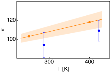
Figure 2: Comparison of the heat conductivities of our LDA-Ar model, as estimated from Green-Kubo and Müller-Plathe ab-initio molecular dynamics. Units are [$\mathrm{mW~{}K^{-1}m^{-1}}$]. Orange: equilibrium (GK) molecular dynamics; the two dots indicate the estimates from our simulations, the straight line their linear inter-/extrapolation. Statistical errors, as estimated by a block analysis of our MD trajectories, are indicated by error bars or by shaded areas, where relevant.

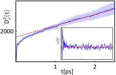
Figure 3: Energy displacement in liquid heavy water at ambient conditions. $D_{e}^{2}(t)\thinspace\mathrm{[10^{-12}mJm^{-1}K^{-1}]}$ was evaluated from the modified flux ${\mathbf{J}^{*}_{e}}=\mathbf{J}_{e}+\lambda^{*}\mathbf{V}$ at $T=\mathrm{385~{}K}$ with a GGA XC functional (see text); the dashed line indicates a linear fit to the large-time behavior of the curve. Inset: integral in the GK relation, $\kappa(t)$ Eq. (1), as a function of the upper limit of integration (see caption to Fig. 1); the dashed line indicates the value of the thermal conductivity obtained from the Einstein relation. i.e. from the slope of above linear fit. The shaded areas depict statistical errors, as estimated from a block analysis of our MD trajectories.

We have applied our newly developed method to compute the heat conductiviy of heavy water at ambient conditions. We have generated a 90-ps long AIMD trajectory for a system of 64 heavy-water molecules in a cubic supercell with an edge of 23.46 a.u., corresponding to the experimental density of 1.11 $\mathrm{g/cm^{3}}$, and at an estimated temperature $\mathrm{T=385\thinspace K}$, using the PBE XC energy functional Perdew:1996 and the PW-PP method as above PP . A time step of 0.0726 fs and a fictitious electronic mass of 340 electron masses were used in this case. The resulting self-diffusion coefficient was estimated to $(2.6\pm 0.2)\times 10^{-5}\thinspace\mathrm{cm^{2}/s}$, to be compared with an experimental value of $2.0\times 10^{-5}\thinspace\mathrm{cm^{2}/s}$ at $T=298\mathrm{\thinspace K}$, following the common practice of comparing experimental data for water at ambient conditions with AIMD-PBE simulations performed at $\sim 400\>\mathrm{K}$ Grossman2004 . The power spectrum of the computed energy flux is characterized by three relatively narrow peaks in correspondence to the intramolecular vibrational modes Silvestrelli:1997 , resulting in long-lived high-frequency oscillations in the integrand of Eq. (1), that plague the evaluation of the integral as a function of the upper limit of integration well beyond the time where the noise of the integrand becomes larger than the amplitude of its oscillations. As the computation of transport coefficients from the Einstein relation Helfand:1960 is less affected by the high-frequency components of the power spectrum Marcolongo:2014 , this ailment is alleviated by evaluating the heat conductivity as the slope of the energy squared displacement, $D_{e}^{2}(t)=\frac{1}{6Vk_{B}T^{2}}\left\langle\left|\int_{0}^{t}\mathbf{J}_{e}(t^{\prime})dt^{\prime}\right|^{2}\right\rangle$, as a function of $t$ in the large-time limit. A direct application of this technique is however not possible as the long-time behavior of the energy squared displacement does not allow us to extrapolate a straight line before it becomes too noisy to analyze. This state of affairs indicates the existence of a slowly decaying mode in the energy-flux correlation function, possibly correlated with a non-diffusive flux. As we have seen, the total velocity $\mathbf{V}$ is such a non-diffusive flux. The value of the corresponding GK conductivity, Eq. (1), however, goes to zero very slowly as a function of the upper limit of integration. This suggests that the slow convergence of the heat conductivity of water as estimated from the slope of the energy squared displacament as a function of time, is possibly due to large correlations existing between the energy flux and the total velocity. We have therefore decided to analyze, instead of $\mathbf{J}_{e}$, the modified flux $\mathbf{J}^{*}_{e}=\mathbf{J}_{e}+\lambda^{*}\mathbf{V}$, where $\lambda^{*}$ has been fixed in such a way as to minimize the correlations between $\mathbf{J}{}_{e}^{*}$ and $\mathbf{V}$. Fig. 2 displays the squared energy displacement computed from $\mathbf{J}_{e}^{*}$ as a function of time and demonstrates that a constant slope can indeed be identified in the long-time limit, giving a value for the heat conductivity of heavy water of $740\pm 120\thinspace\mathrm{mWm^{-1}K^{-1}}$, to be compared with an experimental value of $606\thinspace\mathrm{mWm^{-1}K^{-1}}$ and $595\thinspace\mathrm{mWm^{-1}K^{-1}}$ for light and heavy water respectively at ambient conditions Expt:H2O . The inset displays the behavior of $\kappa(t)$ (see caption to Fig. 1) as a function of the upper limit of integration in the GK formula, indicating that a direct use of Eq. (1) would be extremely difficult in this case. A more detailed error analysis and a systematic extension of this study to different isotopic compositions and other conditions of temperature and pressure is currently in the works.

Conclusions

We believe that the discussion presented in this work will elucidate the scope of a number of assumptions that, although routinely made in the classical simulation of heat transport, have never been fully clarified, thus hampering their generalization to quantum simulations. We are confident that the resulting new methodology will have an impact on important problems where other methods may fail, such as e.g. liquids and glasses, particularly at extreme conditions of temperature and pressure.

Methods

In order to derive Eqs. (5–10), we start from Eq. (4), which we rewrite as:

$$e_{DFT}(\mathbf{r})=e_{KS}(\mathbf{r})+e_{0}(\mathbf{r})+e_{H}(\mathbf{r})+e_{XC}(\mathbf{r}),$$ (13)

where

$$e_{KS}(\mathbf{r}) =\mathrm{Re}\sum_{v}\varphi_{v}^{*}(\mathbf{r})\bigl{(}\hat{H}_{KS}\varphi_{v}(\mathbf{r})\bigr{)},$$ (14)

$$e_{0}(\mathbf{r}) =\sum_{I}\delta(\mathbf{r}-\mathbf{R}_{I})\left(\frac{1}{2}M_{I}V_{I}^{2}+w_{I}\right),$$ (15)

$$e_{H}(\mathbf{r}) =-\frac{1}{2}\rho(\mathbf{r})v_{H}(\mathbf{r}),\qquad\qquad\qquad\text{and}$$ (16)

$$e_{XC}(\mathbf{r}) =\left(\epsilon_{XC}(\mathbf{r})-v_{XC}(\mathbf{r})\right)\rho(\mathbf{r}),$$ (17)

$\epsilon_{XC}$ is a local XC energy per particle, defined by the relation

$$E_{XC}=\int\epsilon_{XC}[\rho](\mathbf{r})\rho(\mathbf{r})d\mathbf{r},$$ (18)

and the XC potential $v_{XC}$ is

$$v_{XC}(\mathbf{r}) =\frac{\delta E_{XC}}{\delta\rho(\mathbf{r})}$$

$$=\epsilon_{XC}(\mathbf{r})+\int\frac{\delta\epsilon_{XC}(\mathbf{r}^{\prime})}{\delta\rho(\mathbf{r})}\rho(\mathbf{r}^{\prime})d\mathbf{r}^{\prime}.$$ (19)

In the LDA, $\epsilon_{XC}$ is a function of the local density, whereas in the GGA it is a function of the local density and density gradients:

$$\epsilon_{XC}^{LDA}[\rho](\mathbf{r}) =\epsilon_{LDA}\bigl{(}\rho(\mathbf{r})\bigr{)},$$ (20)

$$\epsilon^{GGA}_{XC}[\rho](\mathbf{r}) =\epsilon_{GGA}\bigl{(}\rho(\mathbf{r}),\nabla\rho(\mathbf{r})\bigr{)}.$$ (21)

We now proceed to computing the first moments of the time derivatives of the above four densities, according to Eq. (3). In order to simplify the notation, the time dependence of the various quantities will be omitted. Let’s start with the Kohn-Sham energy density, Eq. (14).

$$\dot{e}_{KS}(\mathbf{r}) =\sum_{v}\left(\dot{\varphi}_{v}^{*}(\mathbf{r})\hat{H}_{KS}\varphi_{v}(\mathbf{r})+\varphi_{v}^{*}(\mathbf{r})\hat{H}_{KS}\dot{\varphi}_{v}(\mathbf{r})+\varphi_{v}^{*}(\mathbf{r})\dot{\hat{H}}_{KS}\varphi_{v}(\mathbf{r})\right)$$ (22)

$$=\dot{\bar{e}}_{KS}(\mathbf{r})+\dot{e}^{\prime}_{0}(\mathbf{r})+\dot{e}_{H}^{\prime}(\mathbf{r})+\dot{e}^{\prime}_{XC}(\mathbf{r}),$$ (23)

where

$$\dot{\bar{e}}_{KS}(\mathbf{r}) =\sum_{v}\left[\varepsilon_{v}\dot{\varphi}_{v}^{*}(\mathbf{r})\varphi_{v}(\mathbf{r})+\varphi_{v}^{*}(\mathbf{r})\hat{H}_{KS}\dot{\varphi}_{v}(\mathbf{r})\right],$$ (24)

$$\dot{e}^{\prime}_{0}(\mathbf{r}) =\sum_{v}\varphi_{v}^{*}(\mathbf{r})\dot{\hat{v}}_{0}\varphi_{n}(\mathbf{r}),$$ (25)

$$\dot{e}_{H}^{\prime}(\mathbf{r}) =\dot{v}_{H}(\mathbf{r})\rho(\mathbf{r}),\qquad\text{and}$$ (26)

$$\dot{e}^{\prime}_{XC}(\mathbf{r}) =\dot{v}_{XC}(\mathbf{r})\rho(\mathbf{r}).$$ (27)

The macrosopic flux deriving from $\dot{\bar{e}}_{KS}$, Eq. (24), is the “Kohn-Sham” flux of Eq. (6):

$$\int\mathbf{r}\dot{\bar{e}}_{KS}(\mathbf{r})d\mathbf{r}=\mathbf{J}_{KS}.$$ (28)

The other three terms, Eqs. (25–27) result from the external-, Hartree-, and XC-potential contributions to the time derivative of the KS Hamiltonian (third term in Eq. 22). The corresponding fluxes combine with the fluxes originating from the energy densities of Eqs. (15–17), as explained below.

The first moment of the “ionic potential” energy-density derivative, Eq. (25), reads:

$$\int\mathbf{r}\dot{e}^{\prime}_{0}(\mathbf{r})d\mathbf{r} =\sum_{v}\langle\varphi_{v}|\mathbf{r}\dot{\hat{v}}_{0}|\varphi_{v}\rangle$$

$$=\sum_{v,I}\left\langle\varphi_{v}\left|\mathbf{r}\left(\mathbf{V}_{I}\cdot\nabla_{I}\hat{v}_{0}\right)\right|\varphi_{v}\right\rangle$$

$$=\sum_{v,I}\Bigl{[}\left\langle\varphi_{n}\left|(\mathbf{r}-\mathbf{R}_{I})\left(\mathbf{V}_{I}\cdot\nabla_{I}\hat{v}_{0}\right)\right|\varphi_{n}\right\rangle+\mathbf{R}_{I}\langle\varphi_{v}|(\mathbf{V}_{I}\cdot\nabla_{I}{\hat{v}}_{0})|\varphi_{v}\rangle\Bigr{]}$$

$$=\mathbf{J}^{\prime}_{0}-\sum_{I}\mathbf{R}_{I}\left(\mathbf{V}_{I}\cdot\mathbf{F}_{I}^{el}\right),$$ (29)

where $\mathbf{J}^{\prime}_{0}$ is the flux of Eq. (8), and $\mathbf{F}^{el}_{I}$ is the electronic (Hellmann-Feynman) contribution to the force acting on the $I$-th atom. The corresponding (second) term in the energy flux of Eq. (29) is ill-defined in PBC but, as we will see shortly, it cancels with a similar term coming from the first moment of the “ionic” energy density, Eq. (15).

The time derivative of the “ionic” energy density, Eq. (15), reads:

$$\dot{e}_{0}(\mathbf{r})=\sum_{I}\bigg{[}e^{0}_{I}\,\mathbf{V}_{I}\cdot\nabla_{I}\delta(\mathbf{r}-\mathbf{R}_{I})+\delta(\mathbf{r}-\mathbf{R}_{I})\bigg{(}M_{I}\mathbf{V}_{I}\cdot\dot{\mathbf{V}}_{I}+\sum_{J\neq I}\mathbf{V}_{J}\cdot\nabla_{J}w_{I}\bigg{)}\bigg{]}.$$ (30)

We now use Newton’s equations of motion ($M_{I}\dot{\mathbf{V}}_{I}=\mathbf{F}_{I}$, where $\mathbf{F}_{I}$ is the force acting on the $I$-th atom), and split $\mathbf{F}_{I}$ into an electronic (Hellmann-Feynman) contribution, plus a sum of pair-wise electrostatic terms, $\mathbf{F}_{I}=\mathbf{F}^{el}_{I}-\sum_{J\neq I}\nabla_{I}w_{J}$, to obtain:

$$\int\mathbf{r}\dot{e}_{0}(\mathbf{r})d\mathbf{r} =\sum_{I}\Bigl{[}e^{0}_{I}\mathbf{V}_{I}+\mathbf{R}_{I}\Bigl{(}\mathbf{F}_{I}\cdot\mathbf{V}_{I}+\sum_{J\neq I}\mathbf{V}_{J}\cdot\nabla_{J}w_{I}\Bigr{)}\Bigr{]}.$$

$$=\sum_{I}\Bigl{[}e^{0}_{I}\mathbf{V}_{I}+\mathbf{R}_{I}\left(\mathbf{F}^{el}_{I}\cdot\mathbf{V}_{I}\right)+\mathbf{R}_{I}\sum_{J\neq I}\Bigl{(}\mathbf{V}_{J}\cdot\nabla_{J}w_{I}-\mathbf{V}_{I}\cdot\nabla_{I}w_{J}\Bigr{)}\Bigr{]}$$

$$=\sum_{I}\Bigl{[}e^{0}_{I}\mathbf{V}_{I}+\mathbf{R}_{I}\left(\mathbf{F}^{el}_{I}\cdot\mathbf{V}_{I}\right)+\sum_{J\neq I}(\mathbf{R}_{I}-\mathbf{R}_{J})(\mathbf{V}_{J}\cdot\nabla_{J}w_{I})\bigr{]}$$

$$=\mathbf{J}_{0}+\sum_{I}\mathbf{R}_{I}\left(\mathbf{F}^{el}_{I}\cdot\mathbf{V}_{I}\right),$$ (31)

where $\mathbf{J}_{0}$ is the energy flux of Eq. (9) and the third step follows from the second by interchanging the dummy indeces of one of the two sums over $I$ and $J$. As anticipated before, the second term on the right-hand side of Eq. (31), which is ill-defined in PBC, cancels a similar term in Eq. (29), leaving all the surviving terms well defined. We summarize Eqs. (29) and (31) as:

$$\int\mathbf{r}\bigl{[}\dot{e}_{0}(\mathbf{r})+\dot{e}^{\prime}_{0}(\mathbf{r})\bigr{]}d\mathbf{r}=\mathbf{J}_{0}+\mathbf{J}^{\prime}_{0},$$ (32)

where $\mathbf{J}^{\prime}_{0}$ and $\mathbf{J}_{0}$ are the energy fluxes of Eqs. (8) and (9), respectively.

We then combine the time derivative of the “Hartree” energy density, Eq. (16), with the “Hartree-potential” energy-density derivative, Eq. (26):

$$\dot{\bar{e}}_{H}(\mathbf{r}) =\dot{e}_{H}(\mathbf{r})+\dot{e}^{\prime}_{H}(\mathbf{r})\noindent$$ (33)

$$=\frac{1}{2}\bigl{(}\dot{v}_{H}(\mathbf{r})\rho(\mathbf{r})-\dot{\rho}(\mathbf{r})v_{H}(\mathbf{r})\bigr{)}$$

$$=\frac{1}{8\pi}\bigl{(}v_{H}(\mathbf{r})\Delta\dot{v}_{H}(\mathbf{r})-\dot{v}_{H}(\mathbf{r})\Delta v_{H}(\mathbf{r})\bigr{)}$$

$$=\frac{1}{8\pi}\nabla\cdot\bigl{(}v_{H}(\mathbf{r})\nabla\dot{v}_{H}(\mathbf{r})-\dot{v}_{H}(\mathbf{r})\nabla v_{H}(\mathbf{r})\bigr{)}$$ (34)

Multiplying Eq. (34) by $\mathbf{r}$ and integrating by parts, one obtains:

$$\mathbf{J}_{H} =\int\mathbf{r}\dot{\bar{e}}_{H}(\mathbf{r})d\mathbf{r}$$

$$=\frac{1}{4\pi}\int\dot{v}_{H}(\mathbf{r})\nabla{v}_{H}(\mathbf{r})d\mathbf{r},$$ (35)

which is Eq. (7).

We finally address the first moments of the time derivative of the “XC” energy density, Eq. (17), and of the “XC-potential” energy-density derivative, Eq. (27). We define:

$$\dot{\bar{e}}_{XC}(\mathbf{r}) =\dot{e}_{XC}(\mathbf{r})+\dot{e}^{\prime}_{XC}(\mathbf{r})$$

$$=\bigl{(}\epsilon_{XC}(\mathbf{r})-v_{XC}(\mathbf{r})\bigr{)}\dot{\rho}(\mathbf{r})+\dot{\epsilon}_{XC}(\mathbf{r})\rho(\mathbf{r})$$

$$=\rho(\mathbf{r})\int\frac{\delta\epsilon_{XC}(\mathbf{r})}{\delta\rho(\mathbf{r}^{\prime})}\dot{\rho}(\mathbf{r}^{\prime})d\mathbf{r}^{\prime}-\dot{\rho}(\mathbf{r})\int\frac{\delta\epsilon_{XC}(\mathbf{r}^{\prime})}{\delta\rho(\mathbf{r})}\rho(\mathbf{r}^{\prime})d\mathbf{r}^{\prime},$$ (36)

which derives from the definition of the XC potential, Eq. (19), and from the chain rule as applied to the time derivative of $\epsilon_{XC}$:

$$\dot{\epsilon}_{XC}(\mathbf{r})=\int\frac{\delta\epsilon_{XC}(\mathbf{r})}{\delta\rho(\mathbf{r}^{\prime})}\dot{\rho}(\mathbf{r}^{\prime})d\mathbf{r}^{\prime}.$$ (37)

The first moment of Eq. (36) reads:

$$\mathbf{J}_{XC} =\int\mathbf{r}\dot{\bar{e}}_{XC}(\mathbf{r})d\mathbf{r}$$

$$=\int(\mathbf{r}-\mathbf{r}^{\prime})\rho(\mathbf{r})\dot{\rho}(\mathbf{r}^{\prime})\frac{\delta\epsilon_{XC}(\mathbf{r})}{\delta\rho(\mathbf{r}^{\prime})}d\mathbf{r}d\mathbf{r}^{\prime}.$$ (38)

In the LDA, because of the local dependence of $\epsilon_{XC}$ on the electron density, the functional derivative in Eq. (38) is proportional to $\delta(\mathbf{r}-\mathbf{r}^{\prime})$, thus making the integral vanish. In the GGA Eq. (21) gives:

$$\frac{\delta\epsilon_{XC}^{GGA}(\mathbf{r})}{\delta\rho(\mathbf{r}^{\prime})}=\epsilon^{\prime}_{GGA}(\mathbf{r})\delta(\mathbf{r}-\mathbf{r}^{\prime})\\ +\sum_{\alpha}\partial_{\alpha}\epsilon_{GGA}(\mathbf{r})\nabla_{\alpha}\delta(\mathbf{r}-\mathbf{r}^{\prime}),$$ (39)

where $\epsilon^{\prime}_{GGA}(\mathbf{r})\doteq\left.\frac{\partial\epsilon_{GGA}(\rho,\nabla\rho)}{\partial\rho}\right|_{\rho=\rho(\mathbf{r})}$, and $\partial_{\alpha}\epsilon_{GGA}(\mathbf{r})\doteq\left.\frac{\partial\epsilon_{GGA}(\rho,\nabla\rho)}{\partial\nabla_{\alpha}\rho}\right|_{\rho=\rho(\mathbf{r})}$. The first term on the right-hand side of Eq. (39) does not contribute to the XC energy flux as in the LDA. By inserting the second term into Eq. (38), one finally arrives at the expression for the XC energy flux of Eq. (10), thus completing the derivation of Eqs. (6-10). This rather unwieldy, but all in all straightfoward, derivation is visually summarized in Fig. 4.

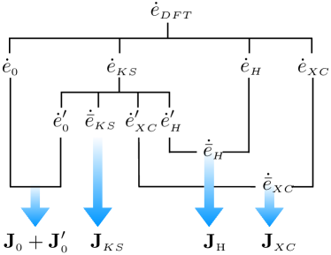
Figure 4: Conceptual flow of the derivation of the various components of the macroscopic energy flux, Eqs. (6-10), from the definition of a microscopic energy density, Eqs. (13-17)

Author contributions

All authors contributed to all aspects of this work.

References

- (1) P. G. Klemens, Thermal conductivity and lattice vibrational modes, Solid State Phys. 7, 1–98 (1958).
- (2) M. S. Green, Markoff random processes and the statistical mechanics of time-dependent phenomena, II. Irreversible processes in fluids, J. Chem. Phys. 22, 398–413 (1954).
- (3) R. Kubo, Statistical-mechanical theory of irreversible processes. I. General Theory and Simple Applications to Magnetic and Conduction Problems, J. Phys. Soc. Jpn. 12, 570–586 (1957).
- (4) D.J. Evans and G. Morriss, Statistical mechanics of nonequilibrium liquids 2nd ed. (Cambridge University Press, Cambridge UK, 2008).
- (5) M. P. Allen and D. J. Tildesley, Computer simulation of liquids (Clarendon Press, Oxford, 1987).
- (6) F. Müller-Plather, A simple nonequilibrium molecular dynamics method for calculating the thermal conductivity, J. Chem. Phys. 106, 6082–6085 (1997).
- (7) R. Car and M. Parrinello, Unified approach for molecular dynamics and density functional theory, Phys. Rev. Lett. 55, 2471–2474 (1985).
- (8) D. Marx and J. Hutter, Ab initio molecular dynamics (Cambridge University Press, Cambridge UK, 2012).
- (9) S. Stackhouse, L. Stixrude, and B. B. Karki, Thermal conductivitity of periclase (MgO) from first principles, Phys. Rev. Lett. 104, 208501 (2010).
- (10) P. Hohenberg and W. Kohn, Inhomogeneous electron gas, Phys. Rev. 136, B864–B871 (1964).
- (11) W. Kohn and L. Sham, Self-consistent equations including exchange and correlation effects, Phys. Rev. 140, A1133–A1138 (1965).
- (12) L. P. Kadanoff and P. C. Martin, Hydrodynamic equations and correlation functions, Ann.Phys. 24, 419–469 (1963).
- (13) D. Forster, Hydrodynamic fluctuations, broken symmetry, and correlation functions (Benjamin, Reading, 1975).
- (14) E. Helfand, Transport coefficients from dissipation in a canonical ensemble, Phys. Rev. 119, 1–9 (1960).
- (15) R. Resta and D. Vanderbilt, Theory of polarization: a modern approach, Top. Appl. Phys. 105, 31–68 (2007).
- (16) N. Chetty and R. M. Martin, First-principles energy density and its applications to selected polar surfaces, Phys. Rev. B 45, 6074–6088 (1992).
- (17) R. Ramprasad, First-principles energy and stress fields in defected materials, J. Phys.: Condens. Matter, 14, 5497–5516 (2002).
- (18) J. P. Perdew, K. Burke, and M. Ernzerhof, Generalized gradient approximation made simple, Phys. Rev. Lett. 77, 3865–3868 (1996).
- (19) D.J. Thouless, Quantization of particle transport, Phys. Rev. B 27, 6083–6087 (1983).
- (20) R. Resta, Manifestations of Berry’s phase in molecules and in condensed matter, J. Phys.: Condens. Matter 12, R107–R143 (2000).
- (21) S. Baroni, S. de Gironcoli, A. Dal Corso, and P. Giannozzi, Phonons and related crystal properties from density-functional perturbation theory, Rev. Mod. Phys. 73, 515–562 (2001).
- (22) P. Giannozzi et al., Quantum ESPRESSO: a modular and open-source software project for quantum simulations of materials, J. Phys.: Condens. Matter 21, 395502 (2009); http://www.quantum-espresso.org.
- (23) CMD simulations have been performed using the LAMMPS code, see: S. Plimpton, Fast parallel algorithms for short-range molecular dynamics, J. Comp. Phys. 117, 1–19 (1995); http://lammps.sandia.gov.
- (24) Norm-conserving PP’s from the Quantum ESPRESSO public repository (http://pseudopotentials.quantum-espresso.org) were used. The PP datasets used for Ar, O, and H are Ar.pz-rrkj.UPF, O.pbe-hgh.UPF, and H.pbe-vbc.UPF, respectively. PW’s up to a kinetic-energy cutoff of 24 Ry for Ar and 80 Ry for water were included in the basis set.
- (25) J.C. Grossman, E. Schwegler, E.W. Draeger, F. Gygi, and G. Galli, Towards an assessment of the accuracy of density functional theory for first principles simulations of water, J. Chem. Phys. 120, 300–311 (2004).
- (26) P. Silvestrelli, M. Bernasconi, and M. Parrinello, Ab initio infrared spectrum of liquid water, Chem. Phys. Lett. 277, 478–482 (1997).
- (27) A. Marcolongo, Theory and ab initio simulation of atomic heat transport, SISSA PhD thesis (2014), http://cm.sissa.it/thesis.php/2014/marcolongo
- (28) N. Matsunaga and A. Nagashima, Transport properties of liquid and gaseous D2O over a wide range of temperature and pressure, J. Phys. Chem. Ref. Data 12, 933–966 (1983); M.L.V. Ramires et al. , Standard reference data for thermal conductivity of water, J. Phys. Chem. Ref. Data 24, 1377–1381 (1994).
Acknowledgements
SB gratefully acknowledges useful discussions with Tao Sun and Dario Alfè in the early phases of this work and, more recently, with Roberto Car and Raffaele Resta. All the authors gratefully thank Luciano Colombo, Claudio Melis, Simon R. Philpot, and Aleksandr Chernatynskiy for commucating to them some of their unpublished material.