Interference Effects in Potential-Wells

Abstract

We propose using an array of potential wells as an interferometer, in which the beam splitters are provided by tunneling during an appropriate time through the barrier between wells. This arrangement allows demonstration of generalized Hong-Ou-Mandel effects with multiple particles traversing one or several beam splitters. Other interferometer effects can occur, including a violation of the Bell-Clauser-Horne-Shimony-Holt form of the Bell inequality. With interactions, one sees various effects including so-called fermionization, collective tunneling, and self-trapping.

^aDepartment of Physics, University of Massachusetts, Amherst, Massachusetts 01003 USA
^b Laboratoire Kastler Brossel, ENS, UPMC, CNRS ; 24 rue Lhomond, 75005 Paris, France

1 Introduction

The Hong-Ou-Mandel (HOM) effect [1, 2] is perhaps the simplest example of boson-boson interference, in which two particles approaching in two different inputs of a beam splitter always exit both in the same output, because destructive interference removes the possibility of exits in separate outputs. Experimental verifications have been carried out with photons [1, 3]. Other cases with two photons from each side [4] as well as two from one side and one from the other have also been considered theoretically [5], and experimentally seen [6]. Theoretical generalizations using cold atoms have recently been considered, including one in which Fock states of arbitrary numbers of particles impinge on a beam splitter [7, 8], and another using pair-correlated atoms produced via a collision of two Bose-Einstein condensates [9]. Recent experiments using particles rather than photons have involved electrons [10], ⁸⁷Rb atoms trapped in optical tweezers [11], and helium atoms [12] where the beam splitter was an Bragg scattering optical grating. Each of the papers using matter waves rather than photons emphasizes that experiments developing coherent indistinguishable pairs of particles may be relevant in other areas such as quantum computing and information processing [13], highly sensitive force detection [14], quantum simulations [15], testing Bell inequalities with material observables [16], etc . Here we want to consider HOM-like interference with the use of Fock states of cold atoms undergoing simple tunneling in optical double (or multiple) potential-wells in a method analogous to that experimentally used in Ref. [11].

The essential element in the HOM effect, or in any interferometer, is a beam splitter. In the case of cold gases, various forms of beam splitter have been designed, including, e.g., Bragg scatterers [12, 17] and double potential-well devices. In the latter case, the usual format [18] involves guiding a matter wave through a potential well having a spatially or temporally growing central repulsive peak that divides the beam into two parts, which, for example, can be recombined further along to show interference effects analogous to a two-slit interferometer. In one case the authors [19] proposed using a pair of side-by-side wave guides having a narrow region where tunneling took place; by adjusting the wave packet width (or momentum) and the barrier width the packet splits into two equal parts, thus using the time of tunneling as the main element to form a 50-50 beam splitter. Recently Daley et al [20] suggested using double-well tunneling as a beam splitter to measure the order-2 Rényi entropy of an entangled state. Compagno et al [21] considered boson and fermion walkers on a one-dimensional lattice with an optical impurity with transmission and reflection coefficients adjusted to act as a beam splitter. Here we will further examine the possible use of the time of tunneling as a beam splitter, a method already adopted by Ref. [11] in their experiment.

Most interference experiments with cold atoms have involved observing a periodicity in the particle density as a function of position or angle. An alternative would be counting the number of particles in the detectors placed after a beam splitter. In the case of the photon HOM experiment a minimum in the coincidence between the two detectors was observed. However, there has been considerable recent progress in the actual observation of individual atoms via the “quantum gas microscope” [22, 23]. In this case the “approach is to assemble quantum information systems with full control over all degrees of freedom, atom by atom, ion by ion” [22]. We will assume such an approach is literally possible so that the number of atoms in each well is known at the beginning of the experiment (input to the beam splitter) and at the end in the detectors after the beam splitters. As in Ref. [11] we assume that the beam splitter involves turning on tunneling between two or more wells for a set time. In this experiment two atoms were trapped in their ground states in wells with optical tweezers and observed via fluorescence. The distance and barrier between the wells could be varied to enhance or cut-off tunneling. In Ref [12] Bragg scattering was used for mirrors and a beam splitter with observation of pairs or singles of atoms falling on a multipixel detector. We will look at variations of the HOM effect but also see that these remarkable experimental methods may yield other interesting possibilities where more elaborate interferometry is possible.

2 Double-well beam splitter

Fig. 1(a) shows a beam splitter with two particle sources and two detectors. In the standard beam splitter with the annihilation operator for source $A$ being $\alpha$ and that for $B$ is $\beta$ then the annihilation operators for detectors 1 and 2 are, respectively

$$d_{1} = \frac{1}{\sqrt{2}}(\alpha+i\beta)$$

$$d_{2} = \frac{1}{\sqrt{2}}(i\alpha+\beta)$$ (1)

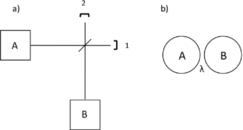
Figure 1: a) $N_{A},N_{B}$ bosons proceed from the sources A and B to a beam splitter, followed by two detectors 1 and 2, where $m_{1}$ and $m_{2}$ particles are detected. b) A double-well potential with tunneling strength $\lambda$ between cells A and B.

We want to show that the the double well of Fig. 1(b) is equivalent to the device of 1(a) if the tunneling occurs for a set time period. Let $a$ be the destruction operator for a particle in well A and $b$ for one in well B. Then the two-level Hamiltonian we consider is taken as

$$H/\hbar=E_{0}(a^{\dagger}a+b^{\dagger}b)-\lambda(a^{\dagger}b+b^{\dagger}a)+\frac{W}{2}(a^{\dagger}a^{\dagger}aa+b^{\dagger}b^{\dagger}bb)$$ (2)

where we have assumed the wells are at equal depth with identical particles in each. The tunneling parameter is $\lambda$ with interactions of strength $W$ among particles in the same well. In the double-well case with no interactions the annhilation operators evolve in time according to

$$a(t) = a(0)\cos\lambda t+ib(0)\sin\lambda t$$

$$b(t) = ia(0)\sin\lambda t+b(0)\cos\lambda t$$ (3)

At time $t=\pi/4\lambda$ we have

$$a\left(\frac{\pi}{4\lambda}\right) = \frac{1}{\sqrt{2}}\left(a(0)+ib(0)\right)=d_{1}$$

$$b\left(\frac{\pi}{4\lambda}\right) = \frac{1}{\sqrt{2}}\left(ia(0)+b(0)\right)=d_{2}$$ (4)

which is then equivalent to the 50-50 beam splitter. The simple two-particle HOM effect, with a single particle initially in each well, corresponds to the following state vector:

$$a^{\dagger}\left(\frac{\pi}{4\lambda}\right)b^{\dagger}\left(\frac{\pi}{4\lambda}\right)\left|0\right\rangle=\frac{1}{2}\left(a(0)^{\dagger}-ib(0)^{\dagger}\right)\left(-ia(0)^{\dagger}+b(0)^{\dagger}\right)\left|0\right\rangle=\frac{-i}{2}\left(a(0)^{\dagger}a(0)^{\dagger}+b(0)^{\dagger}b(0)^{\dagger}\right)\left|0\right\rangle$$ (5)

that is, ending up with a superposition of a pair of particles in each well as expected in the simplest HOM effect. The HOM effect arises because of the destructive interference resulting from exchange of particles in the final state.

For the general case of arbitrary $N$ we can solve for the coefficients in the expansion of the wave function $\left|\psi(t)\right\rangle$ of $H$ in Fock states $\left|n,N-n\right\rangle$, having $n$ particles in well A and $N-n$ in well B. If we take

$$\left|\psi(t)\right\rangle=\sum_{n}c_{n}(t)\left|n,N-n\right\rangle$$ (6)

then the differential equation for $c_{n}(t)$ can be shown to be

$$i\frac{dc_{n}(t)}{dt} = \sum_{n^{\prime}}\left\langle n,N-n\right|H/\hbar\left|n^{\prime},N-n^{\prime}\right\rangle c_{n^{\prime}}(t)$$ (7)

$$= -\lambda\left[\sqrt{n(N-n+1)}c_{n-1}(t)+\sqrt{(n+1)(N-n)}c_{n+1}(t)\right]$$

$$+\frac{W}{2}\left[n^{2}-n+(N-n)^{2}-(N-n)\right]c_{n}(t)$$

where we have omitted the term in $E_{0}$ that leads to a trivial phase factor.

3 HOM calculations

We can use Eqs. (7) to compute HOM-type interferences. For the simplest case of $N_{A}=N_{B}=1,$ the equations are

$$i\dot{c}_{0} = \gamma c_{0}-\sqrt{2}c_{1}$$

$$i\dot{c}_{1} = -\sqrt{2}c_{0}-\sqrt{2}c_{2}$$ (8)

$$i\dot{c}_{2} = \gamma c_{2}-\sqrt{2}c_{1}$$ (9)

where now we have expressed the time in units of $\hbar/\lambda$ and defined $\gamma=W/\lambda.$ The solutions of these equations for the probabilities $|c_{n}(t)|^{2}$ are shown in Fig. 2

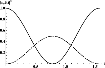
Figure 2: Double-well HOM result with $N=2$, $N_{A}=N_{B}=1,$ showing the time dependence of the probabilities of particle occupation of the wells with no interaction, $\gamma=0$. The probabilities are shown with $|c_{1}(t)|^{2}$ as a solid line, and $|c_{0}(t)|^{2}=|c_{2}(t)|^{2}$, dashed. Initially we assume the wells each contain one particle: $c_{1}(0)=1,$ and $c_{0}(0)=c_{2}(0)=0$. After time $t=\pi/4$ (in units of $\hbar/\lambda$) the probabilities become $|c_{1}|^{2}=0,$ and $|c_{0}|^{2}=|c_{2}|^{2}=1/2.$

For $\gamma=0$ the analytic solutions are

$$c_{0}(t) = c_{2}(t)=\frac{i}{\sqrt{2}}\sin 2t$$

$$c_{1}(t) = \cos 2t$$ (10)

giving the wave function at time $t=\pi/4$ as

$$\left|\psi(t=\pi/4)\right\rangle=\frac{i}{\sqrt{2}}\left(\left|0,2\right\rangle+\left|2,0\right\rangle\right)$$ (11)

Thus the probabilities for the HOM effect, with

$$p_{n}\equiv|c_{n}(\pi/4)|^{2}$$ (12)

are the standard results: $p_{0}=p_{2}=1/2;$ $p_{1}=0.$

This “HOM time” is just as identified in the experiment of Ref. [11], but in our case, the HOM effect can be generalized to more particles in each source as was done in Refs. [7, 8]. In Fig. 3 we show the cases of $N=4$ and 8, where again we consider the occupations of the wells at time $t=\pi/4$ with equal occupation in each well initially.

      

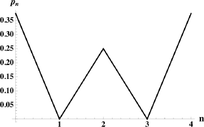
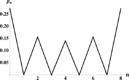
Figure 3: Double-well HOM result with $N=4$ and 8. (Left) Probabilities $p_{n}$ of particle occupation of the well A at time time $t=\pi/4$, for initial conditions $N_{A}=N_{B}=2$; the interaction parameter $\gamma=0$. (Right) Similarly for initial conditions $N_{A}=N_{B}=4.$

If the initial number of particles is not the same in each well then the HOM preference for even occupation can’t be maintained so purely as seen in Fig. 4.

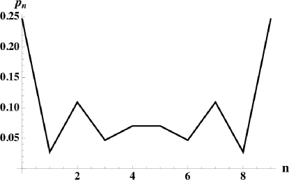
Figure 4: Double-well HOM result for $N=9$, with $N_{A}=4$, $N_{B}=5$ initially, showing the probabilities $p_{n}$ of particle occupation of the well A at time time $t=\pi/4$.

Until now we have reproduced the results of Ref. [7] exactly. One aspect of the present approach to the HOM analysis is that we can include the effects of interactions. In the $N=2$ case the probabilities, gotten from a numerical solution of Eqs. (8), show that $p_{0}$ and $p_{2}$ decrease as $\gamma$ increases and $p_{1}$ increases until all probabilities are equal at $\gamma\approx 2.5$. By $\gamma=6$, $p_{0}$ and $p_{2}$ are very small. This might be expected for a repulsive potential, but the result, (and the Eqs. (7) for any time) are invariant under sign reversal of $\gamma$. The results are the same as if the particles had been fermions. Indeed such so-called fermionization of the system has been seen previously [21, 24]. We can see what is happening by looking at the full time dependence in Fig. 5.

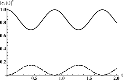
Figure 5: Double-well HOM probabilities $|c_{n}(t)|^{2}$ as a function of time for $N=2$ (initially $N_{A}=N_{B}=1$) with $\gamma=6$; $|c_{0}(t)|^{2}$, $|c_{2}(t)|^{2}$ shown as dashed lines; $|c_{1}(t)|^{2}$ as solid line. Compare with Fig. 2, for which $\gamma=0.$ As $\gamma$ is increased beyond the value here, the amplitudes of the oscillations diminish further.

The average probability for staying in the original {1,1} state is enhanced and those for the pair states {2,0} and {0,2} are diminished. This result illustrates coordinated tunneling as seen in other work [24, 25, 26]. In Refs. [24] and [26] two particles were started out in the same well, and the result was the pair states became favored and the {1,1} state diminished in probability. In our case any coordinated tunneling would seem to involve the pairs crossing together, but in opposite directions, so that we get the opposite result. In Ref. [21] bunching was seen for two non-interacting bosons and antibunching for a pair of fermions or strongly repulsive bosons.

In Fig. 6 we show the effect of increasing $\gamma=W/\lambda$ on the initially equal-sided $N=8$ case. At small $\gamma=0.3$ the HOM effect becomes less “pure” with odd states {1,7},{3,5}, etc now possible; by $\gamma=0.5$ the {4,4} state is enhanced; and at large $\gamma=1$ the {4,4} state has become highly favored. The effect seems related to “self-trapping” in which the sign of an initial imbalance in the number of particles in the two wells becomes fixed when the interaction parameter exceeds a critical value [26, 27, 28, 29, 30], with reduced amplitude oscillations away from the initial value of the imbalance. We discuss some results of an analysis of self-trapping in the Appendix and how our results might be similar. For fixed $N=8$ the critical interaction strength for self-trapping is $\gamma=0.5$; the graphs then show results below, at, and above this critical value. This effect is again independent of the sign of $\gamma.$

            

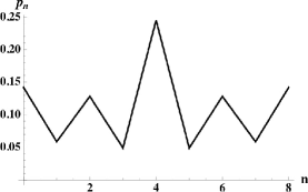
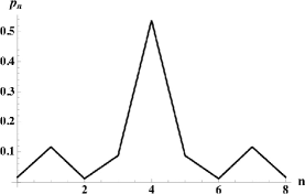
Figure 6: Effects of interactions $\gamma$ on the double-well HOM results with $N=8$. (Cf. Fig. 3(Right)). (Left) Probabilities $p_{n}$ of particle occupation of the well A for initial conditions $N_{A}=N_{B}=4$, and interaction parameter $\gamma=0.3$. (Center) Similarly with $\gamma=0.5$. (Right) Similarly for $\gamma=1.$

4 Generalizations

In addition to simulating a single beam splitter, particle tunneling between wells can behave as an interferometer. Ref. [31] coupled two wave guides together with tunneling at two points, corresponding to beam splitters, to make a two-input, two-output interferometer. Suppose we put three wells in a line as shown in Fig. 7a. Particles in the outer wells A and C are connected by tunneling to the center well B. The tunneling Hamiltonian, without interactions, is

$$H/\hbar=\lambda(a^{\dagger}b+ab^{\dagger}+b^{\dagger}c+bc^{\dagger})$$ (13)

If we solve the equations for $a(t),$ $b(t),$ and $c(t)$ we find that the solutions repeat the initial conditions after a time $t_{R}=\pi/(\sqrt{2}\lambda)$ but at half that, $t_{H}=\pi/(2\sqrt{2}\lambda)$, the equations for the operators are equivalent to detector equations for the interferometer shown in Fig. 7b. Initially we take a single particle in each of the outer wells. The initial configuration repeats in $t_{R}$.

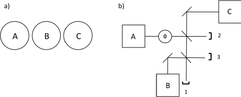
Figure 7: (a) Three wells in a line. (b) The interferometer equivalent to the three-well line of (a). The phase shift needed is $\phi=\pi.$

If a Fock state for the occupation of the three wells is $\left|m_{1},m_{2},m_{3}\right\rangle$, then the wave function at time $t_{H}$ becomes

$$\left|\psi(t_{H})\right\rangle=-\frac{1}{\sqrt{8}}\left|200\right\rangle-\frac{1}{\sqrt{2}}\left|020\right\rangle-\frac{1}{\sqrt{8}}\left|002\right\rangle+\frac{1}{2}\left|101\right\rangle$$ (14)

Thus while the original state $\left|1,0,1\right\rangle$ is present, the only other states are those with two particles in each well, in a kind of HOM effect.

We can place four wells on a square as shown in Fig. 8(a) with particles initially only in wells

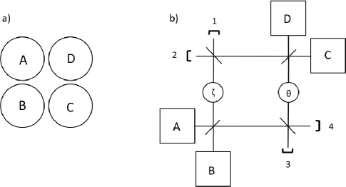
Figure 8: (a) Four wells in a square with tunneling only along the sides. When all four tunneling rates have the same value, $\lambda,$ the system, at $t=\pi/4\lambda$, is equivalent to interferometer shown in (b) with phase shifts $\zeta=\theta=0$.

A and C. Tunneling is between nearest-neighbor wells with the initial state being {A,B,C,D} = {1010}. Possible states are {2000, 0200, 0020, 0002, 1100, 1010, 1001, 0110, 0101, 0011}. Now the repeat time for the initial wave function is $\pi/2\lambda$. At half that, $t_{H}=\pi/4\lambda$, the system is equivalent to the interferometer shown. With a single particle in each of sites A and C, the wave function becomes

$$\left|\psi(t_{H})\right\rangle=-\frac{1}{\sqrt{8}}\left(\left|2000\right\rangle+\left|0200\right\rangle+\left|0020\right\rangle+\left|0002\right\rangle\right)+\frac{1}{2}\left(\left|1010\right\rangle-\left|0101\right\rangle\right)$$ (15)

So in this case the interference removes occupation from these: {1100}, {1001}, {0110}, and {0011}, i.e., states with nearest neighbors both occupied.

However we can do a more interesting experiment with this form of interferometer, namely look at a violation of the Bell theorem. An interferometer method of testing the Bell theorem with arbitrary numbers of bosons was proposed in Ref. [32], with Alice and Bob varying phase angles $\zeta$ and $\theta$ in a device like that in Fig. 8(b). Here we consider the four-well system with just a single particle in each of sites A and C. However, in order to vary the phase angles in the four-well device, we have to allow for variable tunneling rates. Fig. 9 shows how we proceed and defines the variable tunneling rates $\lambda_{1}$ and $\lambda_{2}$.

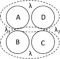
Figure 9: Four wells with Alice’s having counters A and D ; Bob has B and C. The tunneling rate between A and D is $\lambda$ as is that between B and C. The tunneling rate between A and B is $\lambda_{1}$ and that between C and D is $\lambda_{2}.$

After a suitable time, $t=\pi/4\lambda$ we measure the parity product $\left\langle P_{\alpha}P_{\beta}\right\rangle$ with particles in A or C counting positive and those in B or D counting negative so Alice’s parity is $P_{\alpha}=(-1)^{n_{B}}$ and Bob’s is $P_{\beta}=(-1)^{n_{D}}$. We adjust $\lambda_{1}$ and $\lambda_{2}$ to form situations $P_{\alpha}^{\prime}$ and $P_{\beta}^{\prime}$ and maximize the usual quantity in the Bell-Clauser-Horne-Shimony-Holt (BCHSH) form [33] of the Bell theorem: $Q=\left\langle P_{\alpha}P_{\beta}\right\rangle+\left\langle P_{\alpha}^{\prime}P_{\beta}\right\rangle+\left\langle P_{\alpha}P_{\beta}^{\prime}\right\rangle-\left\langle P_{\alpha}^{\prime}P_{\beta}^{\prime}\right\rangle$. Changing the tunneling rate is equivalent to a change of phase in an arm of the interferometer. The tunneling rate $\lambda_{1}$ is Alice’s setting and $\lambda_{2}$ is Bob’s. Denote a parity average by $E(\frac{\lambda_{1}}{\lambda},\frac{\lambda_{2}}{\lambda})$. We maximized $E(1,1)+E(1+\xi,1)+E(1,1-\xi)-E(1+\xi,1-\xi)$ and found the maximum was 2.815 at $\xi=2.74.$ This result is very close to the maximally possible violation of $2\sqrt{2}$ [34].

5 Conclusion

We have shown how a simple set of potential-well traps can be used to demonstrate the HOM effect and to build interferometers where the beam splitter is provided by tunneling between wells. This suggested method emphasizes the possibility of doing generalized HOM experiments with multiple particles by using condensates. The actual implementation of such interference effects involves some requirements that could be difficult: initially counting particle numbers in the wells when used as sources, turning on tunneling for a specified time, and then counting the particle numbers in the wells acting as detectors. Ref. [11] has shown hat these difficulties can be overcome in the $N=2$ case. When interactions among the particles are considered we find the HOM effects change considerably, showing the effects of possible “fermionization”, cooperative pair tunneling, and self-trapping that have been seen in previous double-well analyses. We find that rearranging the wells in various configurations can allow their use as a wide range of interferometers.

After completing our work we learned of related calculations by B. Gertjerenken and P. G. Kevrekidis [35]. We thank them for sharing a preprint with us. We thank Dr. Asaad Sakhel for a critical reading of the manuscript.

Appendix. Self-trapping

We referred to self-trapping as a possible cause of the results shown in Fig. 6. We would like to examine that claim a bit in this appendix. Ref. [28] discusses the dynamics of a Bose-Einstein condensate in a double-well potential and the “self trapping” effect, which occurs when the interactions between particles change the characteristics of the tunneling between the wells. Within a mean-field approximation, free tunneling between wells is reduced for interactions above a certain critical value, causing an initial imbalance between numbers of particles in the wells to be locked in with only smaller amplitude oscillations away from that. In this approximation, all particles occupy the same state given by a Gross-Pitaevskii equation

$$\psi(\mathbf{r})=k_{1}u_{1}(\mathbf{r})+k_{2}u_{1}(\mathbf{r})$$ (16)

where $u_{i}(\mathbf{r})$ represents the groundstate wave function in well $i=1,2.$ The mean-field equations are expressions for the amplitudes $k_{i.}$. When a more exact analysis is used (a full N-body wave function depending on more than two parameters, but still a two-mode approximation), quantum fluctuations alter the mean-field results by time modulations and system revivals.

If we derive equations of motion for the annhilation operators in the Hamiltonian of Eq. (2), we find

$$i\frac{da}{dt} = -b+\gamma a^{\dagger}aa$$

$$i\frac{db}{dt} = -a+\gamma b^{\dagger}bb$$ (17)

where we have measured energy from $E_{0}=0$ and time in units of $\hbar/\lambda$ as before. If we replace $a^{\dagger}a$ by $N_{A}(t)$ and $b^{\dagger}b$ by $N_{B}(t)$ these are just the mean-field equations for the $k_{i}$ found in Ref. [28], which, if one has initial conditions $N_{A}(0)=N$, have the solution [28]

$$N_{A}(t)=\frac{N}{2}\left[1+\mathrm{cn}(2t|N^{2}\gamma^{2}/16)\right]$$ (18)

where $\mathrm{cn}(u|v)$ is a Jacobi elliptic function. An equivalent set of equations suitable for numerical solution for arbitrary initial conditions is given in Ref. [27]. We can compare our own exact results of Eqs. (7) with these mean-field results.

Note that in Sec. 3 our initial condition was always $N_{A}(0)=N_{B}(0).$ In this case one finds in both exact and mean-field cases that $N_{A}(t)=N/2$ because state $\{n,N-n\}$ is always paired in a superposition with state $\{N-n,n\}.$ (Note the symmetry of the probabilities in Fig. 6.) However, self-trapping shows up dramatically when all the particles are initially in one well, $N_{A}(0)=N$. The critical interaction for fixed $N$ is

$$\gamma_{c}=\frac{4}{N}$$ (19)

In Fig. 10 we consider a small value $N=8$, although our equations are valid for any $N$ value. The critical value then is $\gamma_{c}=0.5.$ Our plots show the time dependence of $N_{A}(t).$ For $\gamma=0$ the mean-field and the exact value coincide with a sinusoidal oscillation with full amplitude $0<N_{A}(t)<N$. At $\gamma=0.3<\gamma_{c}$ the mean-field continues to show full oscillation but an additional fluctuation is introduced in the exact result. At critical value $\gamma=0.5$ the mean-field expression reaches self-trapping with $N_{A}(t)=N/2$; the exact result fluctuates about this. (This result favoring equal populations in both wells might be relevant in our own case of Fig. 6.) In the case of $\gamma>\gamma_{c}$ the mean-field result maintains a value of $N_{A}(t)\geq N/2$ with oscillation amplitude decreasing with increasing $\gamma$; the exact quantum value seems to have an additional longer period oscillation frequency superposed, similar to the two-frequency oscillations discussed in Ref. [24].

            

            

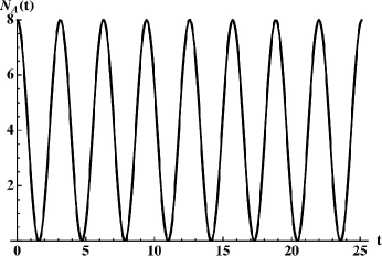
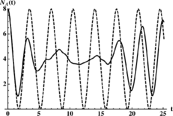
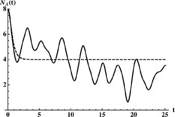
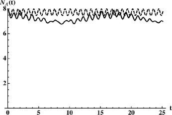
Figure 10: Time dependence of $N_{A}(t)$ in a double-well potential with $N=8$ with initial condition $N_{A}(0)=N$. Solid line, exact result; dashed line, mean-field result of Eq. (18). (Upper Left) No interaction $\gamma=0.$ The exact and mean-field results coincide. (Upper Right) $\gamma=0.3$, below the self-trapping critical interaction value. (Lower Left) $\gamma=0.5$ at the critical value. (Lower Right) $\gamma=1.0$, above the critical value.

If $N_{A}(0)<N$ the amplitude of the oscillation below criticality decreases correspondingly around $N/2.$

None of these results exactly mirrors what we found in Fig. 6, where the configuration {4,4} became favored. In that case, the initial condition was $N_{A}(0)=4$, for which the symmetry of the probabilites leads to $N_{A}(t)=4$, i.e., constant in value, both exactly and in mean-field approximation. However, if we look at the details of the probabilities $p_{n}(t)=\left|c_{n}(t)\right|^{2}$ for individual configurations $\{n,N-n\},$ then we find that the initial configuration itself can become “trapped” at a large value, as seen in Fig. 11 for a large interaction parameter. This effect is analogous to the “fermionization” we saw for just two particles in Fig. 5. This effect is due simply to fact that the initial condition enters with approximately unit amplitude and that any other states are mixed in only in higher order in $1/\gamma$.

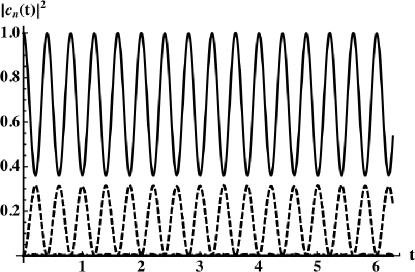
Figure 11: Time dependence of configurations probabilities $\left|c_{n}(t)\right|^{2}$ in a double-well potential with $N=8$ and initial condition $N_{A}(0)=4$ with inteaction $\gamma=10$. The solid line gives $\left|c_{4}(t)\right|^{2}$ for initial configuration $\{4,4\}$, while the dashed line is for $\left|c_{3}(t)\right|^{2}=\left|c_{5}(t)\right|^{2}$ for states $\{3,5\}$ and $\{5,3\}$ respectively. All other states have very small probabilities. The $\{4,4\}$ state is trapped at a relatively large values.

This is an effect that cannot be seen in the mean-field calculations; we plan to return to this subject in a future publication.

References

- [1] C. K. Hong, Z.Y. Ou, L. Mandel, Phys. Rev. Lett. 59, 2044 (1987).
- [2] Z. Y. Ou, Int. J. Mod. Phys., 21, 5033 (2007).
- [3] K. Mattle, H. Weinfurter, P. G. Kwiat, and A. Zeilinger, Phys. Rev. Lett. 76, 4656 (1999); G. Weihs, M. Reck, H. Weinfurter, and A. Zeilinger Phys. Rev. A 54, 893 (1996).
- [4] Z. Y. Ou, J.-K Rhee, and L. J. Wang, Phys. Rev. Lett. 83, 959 (1999).
- [5] H. Wang and T. Kobayashi, Phys. Rev. A 71, 021802(R) (2005).
- [6] K. Sanaka, T. Jennewein, J.-W. Pan, K. Resch, and A. Zeilinger, Phys. Rev. Lett. 92, 017902 (2004).
- [7] F. Laloë and W.J. Mullin, Found. Phys. 42, 53 (2012).
- [8] W. J. Mullin and F. Laloë , Phys. Rev. A 85, 023602 (2012).
- [9] R.J. Lewis-Swan and K.V. Kheruntsyan, Nature Comm. 5, 3752 (2014).
- [10] E. Bocquillon, V. Freulon, J.-M Berroir, P. Degiovanni, B. Plaçais, A. Cavanna, Y. Jin, G. Fève, Science 339, 1054 (2013).
- [11] A. M. Kaufman, B. J. Lester, C. M. Reynolds, M. L. Wall, M. Foss-Feig, K. R. A. Hazzard, A. M. Rey, C. A. Regal, Science 345, 306 (2014).
- [12] R. Lopes, A. Imanaliev, A. Aspect, M. Cheneau, D. Boiron and C. I. Westbrook, Nature 520, 66 (2015).
- [13] P. S. Jessen, I. H. Deutsch, R. Stock, Quant. Info. Proc. 3, 91 (2004).
- [14] V. Giovannetti, S. Lloyd, L. Maccone, Science 306, 1330 (2004).
- [15] I. Bloch, J. Dalibard and S. Nascimbène, Nature Phys. 8, 267 (2012).
- [16] R. J. Lewis-Swan and K. V. Kheruntsyan, http://arxiv.org/abs/1411.0191
- [17] M. Kozuma, L. Deng, E. W. Hagley, J. Wen, R. Lutwak, K. Helmerson, S. L. Rolston, and W. D. Phillips, Phys. Rev. Lett. 82, 871 (1999); A. D. Cronin, J Schmiedmayer, D. E. Pritchard, Rev. Mod. Phys. 81, 1051 (2009); S.-W. Chiow, T. Kovachy, H.-C. Chien, and M. A. Kasevich, Phys. Rev. Lett. 107, 130403 (2011).
- [18] D. Cassettari, B. Hessmo, R. Folman, T. Maier, and J. Schmiedmayer, Phys. Rev. Lett. 85, 5483 (2000); E. A. Hinds, C. J. Vale, and M. G. Boshier, Phys. Rev. Lett. 86, 1462 (2001); W. Hänsel, J. Reichel, P. Hommelhoff, and T. W. Hänsch, Phys. Rev. A 64, 063607 (2001); E. Andersson, T. Calarco, R. Folman, M. Andersson, B. Hessmo, and J. Schmiedmayer, Phys. Rev. Lett. 88, 100401 (2002); Y. Shin, M. Saba, T. A. Pasquini, W. Ketterle, D. E. Pritchard, and A. E. Leanhardt, Phys. Rev. Lett. 92, 050405 (2004); T. Schumm, S. Hofferberth, L. M. Andersson, S. Wildermuth, S. Groth, I. Bar-Joseph, J. Schmiedmayer and P. Krüger, Nature Phys. 1, 57 (2005); L. Pezzé, A. Smerzi, G. P. Berman, A. R. Bishop, and L. A. Collins, Phys. Rev. A 74, 033610 (2006) Berrada, S. van Frank, R. Bücker, T. Schumm, J.-F. Schaff and J Schmiedmayer, Nature Comm. 4, 2077 (2013).
- [19] E. Andersson, M. T. Fontenelle, S. Stenholm, Phys. Rev. A, 59, 3841 (1999).
- [20] A. J. Daley, H. Pichler, J. Schachenmayer, and P. Zoller, Phys. Rev. Lett. 109, 020505 (2012).
- [21] E. Campagno, L. Banchi, and S. Bose, arXiv:1407.8501;L. Banchi, E. Compagno, and S. Bose, arXiv 1502.03061.
- [22] W. S. Bakr, J. I. Gillen, A. Peng, S. Fölling, and M. Greiner, Nature 462, 74 (2009); Barbara Goss Levi, Phys. Today 63, 18 (2010).
- [23] ; J. F. Sherson, C. Weitenberg, M. Endres, M. Cheneau, I. Bloch, and S. Kuhr, Nature 467, 68 (2010).
- [24] S. Zollner, H.-D Meyer, and P. Schmelcher, Phys. Rev. Lett. 100, 040401 (2008) and references therein.
- [25] S. Fölling, S. Trotzky, P. Cheinet, M. Feld, R. Saers, A. Widera, T. Müller, and I. Bloch, Nature 448, 1029 (2007).
- [26] S. Longhi, J. Phys. B: At. Mol. Opt. Phys. 44, 051001 (2011).
- [27] A. Smerzi, S. Fantoni, S. Giovanazzi, and S. R. Shenoy, Phys. Rev. Lett. 79, 4950 (1997).
- [28] G. J. Milburn, J. Corney, E. M. Wright, and D. F. Walls, Phys. Rev. A 55, 4318 (1997).
- [29] M. Albiez, R. Gati, J. Fölling, S. Hunsmann, M. Cristiani, and M. K. Oberthaler, Phys. Rev. Lett. 95, 010402 (2005).
- [30] B. Juliá-Diaz, D. Dagnano, M. Lewenstein, J. Martorell, and A. Polls, Phys. Rev. A 81, 023615 (2010).
- [31] E. Andersson and S. M. Barnett, Phys. Rev. A, 62, 052311 (2000).
- [32] W. J. Mullin and F. Laloë, Phys. Rev. A 78, 061605(R) (2008); F. Laloë, and W. J. Mullin, Eur. Phys. J. B 70, 377 (2009); W. J. Mullin and F. Laloë, Phys. Rev. A 82, 013618 (2010).
- [33] J.F. Clauser, M.A. Horne, A. Shimony, R.A. Holt, Phys. Rev. Lett. 23, 880 (1969).
- [34] B. S. Cirel’son, Lett. Math. Phys. 4, 93 (1980).
- [35] B. Gertjerenken and P. G. Kevrekidis, http://arxiv.org/abs/1503.04316