Join Processing for Graph Patterns:
An Old Dog with New Tricks

Abstract

Join optimization has been dominated by Selinger-style, pairwise optimizers for decades. But, Selinger-style algorithms are asymptotically suboptimal for applications in graphic analytics. This suboptimality is one of the reasons that many have advocated supplementing relational engines with specialized graph processing engines. Recently, new join algorithms have been discovered that achieve optimal worst-case run times for any join or even so-called beyond worst-case (or instance optimal) run time guarantees for specialized classes of joins. These new algorithms match or improve on those used in specialized graph-processing systems. This paper asks can these new join algorithms allow relational engines to close the performance gap with graph engines?

We examine this question for graph-pattern queries or join queries. We find that classical relational databases like Postgres and MonetDB or newer graph databases/stores like Virtuoso and Neo4j may be orders of magnitude slower than these new approaches compared to a fully featured RDBMS, LogicBlox, using these new ideas. Our results demonstrate that an RDBMS with such new algorithms can perform as well as specialized engines like GraphLab – while retaining a high-level interface. We hope our work adds to the ongoing debate of the role of graph accelerators, new graph systems, and relational systems in modern workloads.

1 Introduction

For the last four decades, Selinger-style pairwise-join enumeration has been the dominant join optimization paradigm [13]. Selinger-style optimizers are designed for joins that do not filter tuples, e.g., primary-key-foreign-key joins that are common in OLAP. Indeed, the result of a join in an OLAP query plan is often no smaller than either input relation. In contrast, in graph applications, queries search for structural patterns, which filter the data. These regimes are quite different, and not surprisingly there are separate OLAP and graph-style systems. Increasingly, analytics workloads contain both traditional reporting queries and graph-based queries [12]. Thus, it would be desirable to have one engine that is able to perform well for join processing in both of these different analytics settings.

Unifying these two approaches is challenging both practically and theoretically. Practically, graph engines offer orders of magnitude speedups over traditional relational engines, which has led many to conclude that these different approaches are irreconcilable. Indeed, this difference is fundamental: recent theoretical results suggest that Selinger-style, pair-wise join optimizers are asymptotically suboptimal for this graph-pattern queries [9, 15, 3]. The suboptimality lies in the fact that Selinger-style algorithms only consider pairs of joins at a time, which leads to runtimes for cyclic queries that are asymptotically slower by factors in the size of the data, e.g., $\Omega(\sqrt{N})$-multiplicative factor worse on a database with $N$ tuples. Nevertheless, there is hope of unifying these two approaches for graph pattern matching as, mathematically, (hyper)graph pattern matching is equivalent to join processing. Recently, algorithms have been discovered that have strong theoretical guarantees, such as optimal runtimes in a worst-case sense or even instance optimally. As database research is about three things: performance, performance, and performance, the natural question is:

To what extent do these new join algorithms speed up graph workloads in an RDBMS?

To take a step toward answering this question, we embed these new join algorithms into the LogicBlox (LB) database engine, which is a fully featured RDBMS that supports rich queries, transactions, and analytics. We perform an experimental comparison focusing on a broad range of analytics workloads with a large number of state-of-the-art systems including row stores, column stores, and graph processing engines. Our technical contribution is the first empirical evaluation of these new join algorithms. At a high-level, our message is that these new join algorithms provide substantial speedups over both Selinger-style systems and graph processing systems for some data sets and queries. Thus, they may require further investigation for join and graph processing.

We begin with a brief, high-level description of these new algorithms, and then we describe our experimental results.

An Overview of New Join Algorithms

Our evaluation focuses on two of these new-style algorithms, LeapFrog TrieJoin (LFTJ) [15], a worst-case optimal algorithm, and Minesweeper (MS), a recently proposed “beyond-worst-case” algorithm [8].

LFTJ is a multiway join algorithm that transforms the join into a series of nested intersections. LFTJ has a running time that is worst-case optimal, which means for every query there is some family of instances so that any join algorithm takes as least much time as LFTJ does to answer that query. These guarantees are non-trivial; in particular, any Selinger-style optimizer is slower by a factor that depends on the size of the data, e.g., by a factor of $\Omega(\sqrt{N})$ on a database with $N$ tuples. Such algorithms were discovered recently [9, 15], but LFTJ has been in LogicBlox for several years.

Minesweeper’s main idea is to keep careful track of every comparison with the data to infer where to look next for an output. This allows Minesweeper to achieve a so-called “beyond worst-case guarantee” that is substantially stronger than a worst-case running time guarantees: for a class called comparison-based algorithms, containing all standard join algorithms including LFTJ, beyond worst-case guarantees that any join algorithm takes no more than a constant factor more steps on any instance. Due to indexing, the runtime of some queries can even be sublinear in the size of the data. However, these stronger guarantees only apply for a limited class of acyclic queries (called $\beta$-acyclic).

Benchmark Overview

The primary contribution of this paper is a benchmark of these new style algorithms against a range of competitor systems on graph-pattern matching workloads. To that end, we select a traditional row-store system (Postgres), a column-store system (MonetDB) and graph systems (virtuoso, neo4j, and graphlab). We find that for cyclic queries these new join systems are substantially faster than relational systems and competitive with graph systems. We find that LFTJ is performant in cyclic queries on dense data, while Minesweeper is superior for acyclic queries.

Contributions

This paper makes two contributions:

1. We describe the first practical implementation of a beyond worst-case join algorithm.

2. We perform the first experimental validation that describes scenarios for which these new algorithms are competitive with conventional optimizers and graph systems.

2 Background

We recall background on graph patterns, join processing, and hypergraph representation of queries along with the two new join algorithms that we consider in this paper.

2.1 Join query and hypergraph representation

A (natural) join query $Q$ is specified by a finite set $\mathrm{atoms}(Q)$ of relational symbols, denoted by $Q=\ \Join_{R\in\mathrm{atoms}(Q)}R$. Let $\textnormal{vars}(R)$ denote the set of attributes in relation $R$, and

$$\textnormal{vars}(Q)=\bigcup_{R\in\mathrm{atoms}(Q)}\textnormal{vars}(R).$$

Throughout this paper, let $n=|\textnormal{vars}(Q)|$ and $m=|\mathrm{atoms}(Q)|$. For example, in the following so-called triangle query

$$Q_{\triangle}=R(A,B)\Join S(B,C)\Join T(A,C).$$

we have $\textnormal{vars}(Q_{\triangle})=\{A,B,C\}$, $\textnormal{vars}(R)=\{A,B\}$, $\textnormal{vars}(S)=\{B,C\}$, and $\textnormal{vars}(T)=\{A,C\}$. The structure of a join query $Q$ can be represented by a hypergraph $\mathcal{H}(Q)=(\mathcal{V},\mathcal{E})$, or simply $\mathcal{H}=(\mathcal{V},\mathcal{E})$. The vertex set is $\mathcal{V}=\textnormal{vars}(Q)$, and the edge set is defined by

$$\mathcal{E}=\left\{\textnormal{vars}(R)\ |\ R\in\mathrm{atoms}(Q)\right\}.$$

Notice that if the query hypergraph is exactly finding a pattern in a graph. For so-called $\alpha$-acyclicity [4, 2], the celebrated Yannakakis algorithm [17] runs in linear-time (in data complexity). On graph databases with binary relations, both $\alpha-$ and $\beta-$ acyclic can simply be thought of as the standard notion of acyclic.

Worst-case Optimal Algorithm

Given the input relation sizes, Atserias, Grohe, and Marx [3] derived a linear program that could be used to upper bound the worst-case (largest) output size in number of tuples of a join query. For a join query, $Q$ we denote this bound $\textsf{AGM}(Q)$. For completeness, we describe this bound in Appendix A. Moreover, this bound is tight in the sense that there exists a family of input instances for any $Q$ whose output size is $\Omega(\textsf{AGM}(Q))$. Then, Ngo, Porat, Ré, and Rudra (NPRR) [9] presented an algorithm whose runtime matches the bound. This algorithm is thus worst-case optimal. Soon after, Veldhuizen [15] used a similar analysis to show that the LFTJ algorithm – a simpler algorithm already implemented in LogicBlox Database engine – is also worst-case optimal. A simpler exposition of these algorithms was described [10] and formed the basis of a recent system [1].

Beyond Worst-case Results

Although NPRR may be optimal for worst-case instances, there are instances on which one can improve its runtime. To that end, the tightest theoretical guarantee is so-called instance optimality which says that the algorithm is up to constant factors no slower than any algorithm, typically, with respect to some class of algorithms. These strong guarantees had only been known for restricted problems [5]. Recently, it was shown that if the query is $\beta$-acyclic, then a new algorithm called Minesweeper (described below) is $\log$-instance optimal with respect to the class of comparison-based joins, a class which includes essentially all known join and graph processing algorithms. Theoretically, this result is much stronger–but this algorithm’s performance not been previously reported in the literature.

2.2 The Leapfrog Triejoin Algorithm

We describe the Leapfrog Triejoin algorithm. The main idea is to “leapfrog” over large swaths of tuples that cannot produce output. To describe it, we need some notation. For any relation $R$, an attribute $A\in\textnormal{vars}(R)$, and a value $a\in\pi_{A}(R)$, define

$$R[a]=\pi_{\textnormal{vars}(R)-\{A\}}(\sigma_{A=a}(R)).$$

That is $R[a]$ is the set of all tuples from $R$ whose $A$-value is $a$.

At a high-level, the Leapfrog Triejoin algorithm can be presented recursively as shown in Algorithm 1. In the actual implementation, we implement the algorithm using a simple iterator interface, which iterates through tuples. Please see Section 3 for more detail.

Algorithm 1 High-level view: Leapfrog Triejoin ($\textsf{LFTJ}(Q)$)

1:All relations $R$ are in $\mathrm{atoms}(Q)$

2:Let $\textnormal{vars}(Q)=(A_{1},\dots,A_{n})$

3:$L\leftarrow\bigcap_{R:A_{1}\in\textnormal{vars}(R)}\pi_{A_{1}}(R)$

4:if $n=1$ then

5:     return $L$

6:for each $a_{1}\in L$ do

7:     $\triangleright$ The following forms a new query on $(A_{2},\dots,A_{n})$

8:     $Q_{a_{1}}\leftarrow\bigl{(}\Join_{R:A_{1}\in\textnormal{vars}(R)}R[a_{1}]\Join\Join_{R:A_{1}\notin\textnormal{vars}(R)}R\bigr{)}$

9:

10:     $S_{a_{1}}=\textsf{LFTJ}(Q_{a_{1}})$ $\triangleright$ Recursive call

11:return $\bigcup_{a_{1}\in L}\{a_{1}\}\times S_{a_{1}}$

One can show that the Leapfrog Triejoin (LFTJ) algorithm runs in time $\tilde{O}(N+\textsf{AGM}(Q))$ for any query $Q$ [15]. The simplified version shown above appeared later [10].

2.3 The Minesweeper Algorithm

Consider the set of tuples that could be returned by a join (i.e., the cross products of all domains). Often many fewer tuples are part of the output than are not. Minesweeper’s exploits this idea to focus on quickly ruling out where tuples are not located rather than where they are. Minesweeper starts off by obtaining an arbitrary tuple $\mathbf{t}\in\mathbb{N}^{\textnormal{vars}(Q)}$ from the output space, called a free tuple (also called a probe point in [8]). By probing into the indices storing the input relations, we either confirm that $\mathbf{t}$ is an output tuple or we get back $\tilde{O}(1)$ “gaps” or multi-dimensional rectangles inside which we know for sure no output tuple can reside. We call these rectangles gap boxes. The gap boxes are then inserted into a data structure called the constraint data structure (CDS). If $\mathbf{t}$ is an output tuple, then a corresponding (unit) gap box is also inserted in to the CDS. The CDS helps compute the next free tuple, which is a point in the output space not belonging to any stored gap boxes. The CDS is a specialized cache that ensures that we maximally use the information we gather about which tuples must be ruled out. The algorithm proceeds until the entire output space is covered by gap boxes. Algorithm 2 gives a high-level overview of how Minesweeper works.

Algorithm 2 High-level view: Minesweeper algorithm

1:$\text{CDS}\leftarrow\emptyset$ $\triangleright$ No gap discovered yet

2:while CDS can find $\mathbf{t}$ not in any stored gap do

3:     if $\pi_{\textnormal{vars}(R)}(\mathbf{t})\in R$ for every $R\in\mathrm{atoms}(Q)$ then

4:         Report $\mathbf{t}$ and insert $\mathbf{t}$ as a gap into CDS

5:     else

6:         Query all $R\in\mathrm{atoms}(Q)$ for gaps around $\mathbf{t}$

7:         Insert those gaps into CDS      

A key idea from [8] was the proof that the total number of gap boxes that Minesweeper discovers using the above outline is $\tilde{O}(|\mathcal{C}|)$, where $\mathcal{C}$ is the minimum set of comparisons that any comparison-based algorithm must perform in order to work correctly on this join. Essentially all existing join algorithms such as Block-Nested loop join, Hash-Join, Grace, Sort-merge, index-nested, PRISM, double pipelined, are comparison-based (up to a $\log$-factor for hash-join). For $\beta$-acyclic queries, Minesweeper is instance optimal up to an (unavoidable) $\log N$ factor.

3 LogicBlox Database System

The LogicBlox database is a commercial database system that from the ground up is designed to serve as a general-purpose database system for enterprise applications. The LogicBlox database is currently primarily used by partners of LogicBlox to develop applications that have a complex workload that cannot easily be categorized as either analytical, transactional, graph-oriented, or document-oriented. Frequently, the applications also have a self-service aspect, where an end-user with some modeling expertise can modify or extend the schema dynamically to perform analyses that were originally not included in the application.

The goal of developing a general-purpose database system is a deviation from most current database system development, where the emphasis is on designing specialized systems that vastly outperform conventional database systems, or to extend one particular specialization (e.g. analytical) with reasonable support for a different specialized purpose (e.g. transactional).

The challenging goal of implementing a competitive general-purpose database, requires different approaches in several components of a database system. Join algorithms are a particularly important part, because applications that use LogicBlox have schemas that resemble graph as well as OLAP-style schemas, and at the same time have a challenging transactional load. To the best of our knowledge, no existing database system with conventional join algorithms can efficiently evaluate queries over such schemas, and that is why LogicBlox is using a join algorithm with strong optimality guarantees: LFTJ.

Concretely, the motivation for implementing new optimal join algorithms are:

• No previously existing join algorithm efficiently supports the graph queries required in applications. On the other hand, graph-oriented systems cannot handle OLAP aspects of applications.

• To make online schema changes easy and efficient, LogicBlox applications use unusually high normalization levels, typically 6NF. The normalized schemas prevent the need to do surgery on existing data when changing the schema, and also helps with efficiency of analytical workloads (compare to column stores). A drawback of this approach is that queries involve a much larger number of tables. Selection conditions in queries typically apply to multiple tables, and simultaneously considering all the conditions that narrow down the result becomes important.

• As opposed to the approach of highly tuned in-memory databases that fully evaluate all queries on-the-fly [12], LogicBlox encourages the use of materialized views that are incrementally maintained [14]. The incremental maintenance of the views under all update scenarios is a challenging task for conventional joins, in particular combined with a transactional load highly efficient maintenance is required [16].

The LogicBlox database system is designed to be highly modular as a software engineering discipline, but also to encourage experimentation. Various components can easily be replaced with different implementations. This enabled the implementation of Minesweeper, which we compare to the LFTJ implementation and other systems in this paper.

4 Minesweeper implementation

4.1 Global attribute order (GAO)

Both Leapfrog Triejoin and Minesweeper work on input relations that are already indexed using a search-tree data structure such as a traditional B-tree which is widely used in commercial relational database systems [11, Ch.10]. For example, Figure 1 shows the index for a relation $R$ on attribute set $\textnormal{vars}(R)=\{A_{2},A_{4},A_{5}\}$. This index for $R$ is in the order $A_{2},A_{4},A_{5}$.

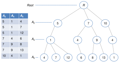
Figure 1: How Minesweeper “views” input indices

Furthermore, there is an ordering of all the attributes in $\textnormal{vars}(Q)$ – called the global attribute order (GAO) – such that all input relations are indexed consistent with this GAO. This assumption shall be referred to as the GAO-consistency assumption. For example, for the triangle query $Q=R(A,B)\Join S(B,C)\Join T(A,C)$, if the GAO is $B,A,C$, then $R$ is indexed in the $(B,A)$ order, $S$ in the $(B,C)$, and $T$ in the $(A,C)$.

4.2 Gap boxes, constraints, and patterns

To describe the gap boxes, let us consider an example. Suppose $\textnormal{vars}(Q)=\{A_{0},A_{1},\dots,A_{6}\}$ with $(A_{0},A_{1},A_{2},\dots,A_{6})$ being the GAO. Suppose the relation $R$ shown in Figure 1 is an input relation. Consider the following free tuple

$$\mathbf{t}=(t_{0},t_{1},t_{2},t_{3},t_{4},t_{5},t_{6})=(2,6,6,1,3,7,9).$$

We first project this tuple down to the coordinate subspace spanned by the attributes of $R$: $(t_{2},t_{4},t_{5})=(6,3,7)$. From the index structure for $R$, we see that $t_{2}=6$ falls between the two $A_{2}$-values $5$ and $7$ in the relation. Thus, this index returns a gap consisting of all points lying between the two hyperplanes $A_{2}=5$ and $A_{2}=7$. This gap is encoded with the constraint

$$\mathbf{c}=\langle*,*,(5,7),*,*,*,*\rangle,$$ (1)

where $*$ is the wildcard character matching any value in the corresponding domain, and $(5,7)$ is an open interval on the $A_{2}$-axis. On the other hand, suppose the free tuple is

$$\mathbf{t}=(t_{0},t_{1},t_{2},t_{3},t_{4},t_{5},t_{6})=(2,6,7,1,5,8,9).$$

Then, a gap returned might be the band in the hyperplane $A_{2}=7$,  $4<A_{4}<9$. The encoding of this gap is

$$\mathbf{c}^{\prime}=\langle*,*,7,*,(4,9),*,*\rangle.$$ (2)

The number $7$ indicates that this gap is inside the hyperplane $A_{2}=7$, and the open interval encodes all points inside this hyperplane where $4<A_{4}<9$.

Due to the GAO-consistency assumption, all the constraints returned by the input indices have the property that for each constraint there is only one interval component, after that there are only wildcard component.

Definition 4.1 (Constraint and pattern).

Gap boxes are encoded by constraints. Each constraint is an $n$-dimensional tuple $\mathbf{c}=\langle c_{0},\dots,c_{n-1}\rangle$, where each $c_{i}$ is either a member of $\mathbb{N}\cup\{*\}$ or an open interval $(\ell,r)$ where $\ell,r\in\mathbb{N}$. For each constraint $\mathbf{c}=\langle c_{0},\dots,c_{n-1}\rangle$, there is only one $c_{i}$ which is an interval, after which all components are wildcards. The tuple of components before the interval component is called the pattern of the constraint, denoted by $\textsf{pattern}(\mathbf{c})$. For example, $\textsf{pattern}(\mathbf{c})=\langle*,*\rangle$ for the constraint $\mathbf{c}$ defined in (1), and $\textsf{pattern}(\mathbf{c}^{\prime})=\langle*,*,7,*\rangle$ for the constraint in (2).

4.3 The constraint data structure (CDS)

Figure 2: Example of the ConstraintTree data structure for $n=5$. The top left figure is the CDS after the constraint $\langle*,*,(5,7),*,*\rangle$ is inserted into an empty CDS. The top right is the CDS after $\langle*,*,7,*,(4,9)\rangle$ was added. The bottom figure is the CDS after the following constraints are further added: $\langle*,1,(1,3),*,*\rangle,\langle*,1,(9,10),*,*\rangle,\langle*,1,2,(10,19),*\rangle,\langle*,1,3,5,(3,9)\rangle$, $\langle*,1,3,5,(1,3)\rangle,\langle*,1,3,5,(10,14)\rangle,\langle*,1,3,*,(5,10)\rangle$.

The CDS is a data structure that implements two functions as efficiently as possible: (1) $\textsc{InsConstraint}(\mathbf{c})$ takes a new constraint $\mathbf{c}$ and inserts it into the data structure, and (2) computeFreeTuple computes a tuple $\mathbf{t}$ that does not belong to any constraints (i.e. gap boxes) that have been inserted into the CDS. computeFreeTuple returns true if $\mathbf{t}$ was found, and false otherwise.

To support these operations, we implement the CDS using a tree data structure with at most $n$ levels, one for each of the attributes following the GAO. Figure 2 illustrates such a tree.

For each node $v\in\text{CDS}$, there are two important associated lists: $v.\textsf{child}$ and $v.\textsc{intervals}$.

• $v.\textsf{child}$ is a map from $\mathbb{N}\cup\{*\}$ to children nodes of $v$ in the CDS, where each parent-child edge is labeled with a label in $\mathbb{N}\cup\{*\}$. In particular, $v.\textsf{child}[a]$ is the child node $u$ of $v$, where the $vu$ edge is labeled with $a$. Consequently, each node $v$ in the CDS is identified by the tuple of labels of edges from the root to $v$. Naturally we call this tuple of labels $\textsf{pattern}(v)$. It is certainly possible for $v.\textsf{child}=\emptyset$, in which case $v$ is a leaf node of the CDS. (See Figure 2 for an illustration.)

• $v.\textsc{intervals}$ is a set of disjoint open intervals of the form $(\ell,r)$, where $\ell,r\in\mathbb{N}\cup\{-\infty,+\infty\}$. Each interval $(\ell,r)\in v.\textsc{intervals}$ corresponds to a constraint $\mathbf{c}=\langle\textsf{pattern}(v),(\ell,r),*,\dots,*\rangle$. In particular, when we insert new intervals into $v.\textsc{intervals}$, overlapped intervals are automatically merged.

Idea 1 (Point List).

To implement the above lists, we used one single list for each node called the pointList. For each node $v$ of the CDS, $v.\textsf{pointList}$ is a (sorted) subset of $\mathbb{N}\cup\{-\infty,+\infty\}$. Each value $x\in v.\textsf{pointList}$ has a set of associated data members, which tells us whether $x$ is a left end point, right end point of some interval in $v.\textsc{intervals}$, or both a left end point of some interval and the right end point of another. For example, if $(1,10)$ and $(10,20)$ are both in $v.\textsc{intervals}$, then $x=10$ is both a left and a right end point. The second piece of information is a pointer to another node of the CDS. If $v.\textsf{child}[x]$ exists then this pointer points to that child, otherwise the pointer is set to . The pointList is made possible by the fact that when newly inserted intervals are not only merged with overlapping intervals, but also eliminate children nodes whose labels are inside the newly inserted interval. We will see later that the pointList adds at least two other benefits for speeding up Minesweeper and #Minesweeper.

With the above structure, inserting a constraint into the CDS is straightforward. In the next section we describe the computeFreeTuple algorithm which is the most important algorithm to make Minesweeper efficient. There are two additional simple functions associated with each node $v$ in the CDS that are used often in implementing computeFreeTuple:

• $v.\textsf{Next}(\texttt{int }x)$ returns the smallest integer $y\geq x$ such that $y$ does not belong to any interval in the list $v.\textsc{intervals}$.

• $v.\textsf{hasNoFreeValue}()$ returns whether $v.\textsf{Next}(-1)=+\infty$, i.e. all values in $\mathbb{N}$ are covered by intervals in $v.\textsc{intervals}$.

4.4 A slight change to computeFreeTuple

Idea 2 (The moving frontier).

While basic Minesweeper (Algorithm 2) states that a new free tuple $\mathbf{t}$ is computed afresh at each outer loop of the algorithm, this strategy is inefficient. In our implementation, we move free tuples in lexicographically increasing order which speeds up the algorithm because some constraints can be implicit instead of explicitly inserted into the CDS.

More concretely, the CDS maintains a tuple $\textsc{curFrontier}\in\mathbb{N}^{n}$ called the frontier. We start with $\textsc{curFrontier}=(-1,-1,\dots,-1)$. In the computeFreeTuple function, the CDS has to compute the next free tuple $\mathbf{t}$ which is greater than or equal to the frontier in lex order and – of course – does not satisfy any of the constraint stored in the CDS. In particular, all tuples below the frontier are either implicitly ruled out or are output tuples which have already been reported.

This idea has a very important benefit. When the current free tuple is verified to be an output tuple, then we do not need to insert a new constraint just to rule out a single tuple in the output space! (If we were to insert such a constraint, it would be of the form $\langle t_{0},\dots,t_{n-2},(t_{n-1}-1,t_{n-1}+1)\rangle$, which adds a very significant overhead in terms of space and time as many new pointers are allocated.) Instead, we change the frontier to be $\textsc{curFrontier}=(t_{0},\dots,t_{n-2},t_{n-1}+1)$ and ask the CDS for the next free tuple.

4.5 Obtaining gaps from relations

Idea 3 (Geometric certificate).

The key notion of comparison certificate from [8] was the set $\mathcal{C}$ of comparisons that any comparison-based algorithm must discover to certify the correctness of its output. In order to show that Minesweeper (as outlined in Algorithm 2) inserts into the CDS $\tilde{O}(|\mathcal{C}|)$ many constraints, the gaps were crafted carefully in [8] so that in each iteration at least one comparison in $\mathcal{C}$ is “caught.”

Let us forget about the Boolean notion of comparison certificate for now and examine what the CDS sees and processes. The CDS has a set of output boxes, and a collection of gap boxes which do not contain any output point. When the CDS cannot find a free tuple anymore, the union of output boxes and gap boxes is the entire output space. In other words, every point in the output space is either an output point, or is covered by a gap box. We will call the collection of gap boxes satisfying this property a box certificate, denoted by $\mathcal{C}_{\Box}$. A box certificate is a purely geometric notion, and on the surface does not seem to have anything to do with comparisons. Yet from the results in [8], we now know that a box certificate of minimum size is a lowerbound on the number of comparisons issued by any comparison-based join algorithm (with the GAO-assumption).

With this observation in mind, for every free tuple $\mathbf{t}$, we only need to find from each relation $R$ the maximal gap box containing the projection $\pi_{\textnormal{vars}(R)}(\mathbf{t})$, and if $\pi_{\textnormal{vars}(R)}(\mathbf{t})\in R$ then no gap box is reported. Suppose $R$ has $k$ attributes $A_{i_{1}},\dots,A_{i_{k}}$, for $i_{1}<\dots<i_{k}$, and suppose $\pi_{\textnormal{vars}(R)}(\mathbf{t})\notin R$, the maximal gap box from $R$ with respect to the free tuple $\mathbf{t}$ is found as follows. Let $j\in[k]$ be the smallest integer such that

$$\pi_{A_{i_{1}},\dots,A_{i_{j-1}}}(\mathbf{t})\in\pi_{A_{i_{1}},\dots,A_{i_{j-1}}}(R)\text{ and }\pi_{A_{i_{1}},\dots,A_{i_{j}}}(\mathbf{t})\notin\pi_{A_{i_{1}},\dots,A_{i_{j}}}(R).$$

To shorten notations, write $J=\pi_{A_{i_{1}},\dots,A_{i_{j}}}(R)$ and define

$$\ell = \max\{x\in\mathbb{N}\cup\{-\infty\}\ |\ x<t_{i_{j}}\wedge(t_{i_{1}},\dots,t_{i_{j-1}},x)\in J\}$$

$$r = \min\{x\in\mathbb{N}\cup\{+\infty\}\ |\ x>t_{i_{j}}\wedge(t_{i_{1}},\dots,t_{i_{j-1}},x)\in J\}.$$

Then, the constraint from $R$ is $\mathbf{c}_{R}=\langle c_{0},\dots,c_{n-1}\rangle$ where

$$c_{i}=\begin{cases}*&\text{ if }i\notin\{i_{1},\dots,i_{j}\}\\ t_{i_{p}}&\text{ if }i=i_{p}\wedge p<j\\ (\ell,r)&\text{ if }i=i_{j}.\end{cases}$$

Idea 4 (Avoid repeated seekGap()).

To find a constraint as described above from a relation $R$, we use the operators seek_lub() (least upper bound) and seek_glb() (greatest lower bound) from LogicBlox’ Trie index interface. These operations are generally costly in terms of runtime as they generally require disk I/O. Hence, we try to reduce the number of calls to seek_gap() whenever possible. In particular, for each constraint inserted into the CDS, we record which relation(s) it came from. For example, suppose we have a relation $R(B,C)$ which has inserted a constraint $\langle*,b,(\ell,r)\rangle$ to the CDS. Then, when the free tuple is $\mathbf{t}=(a,b,r)$, we knew that no gap can be found from $R$ without calling any seek_gap() on $R$. This simple idea turns out to significantly reduce the overall runtime of Minesweeper. The speedup when this idea is incorporated is shown in Table 1.

- ca-GrQc p2p-Gnutella04 facebook ca-CondMat wiki-vote p2p-Gnutella31 email-Enron loc-brightkite soc-Epinions1 soc-Slashdot0811 soc-Slashdot0902 twitter-combined Idea 4 2-comb 1.38 1.34 1.82 1.54 2.24 1.26 2.06 2.02 2.13 2.30 2.26 2.55 3-path 1.11 1.26 1.72 1.46 1.94 1.24 1.83 1.59 1.93 2.26 2.08 2.54 4-path 1.37 1.45 1.81 1.86 2.06 1.35 2.12 2.10 2.09 2.21 2.19 2.71 Ideas 4&6 2-comb 1.51 1.48 2.60 1.69 3.46 1.35 3.30 2.98 3.36 4.16 4.11 4.49 3-path 1.10 1.42 2.13 1.50 2.82 1.27 2.50 1.91 3.13 3.79 3.64 4.52 4-path 1.74 1.49 2.56 2.15 3.34 1.43 3.58 3.26 3.08 3.97 3.93 5.18

Table 1: Speedup ratio when Ideas 4 and 6 are incorporated

4.6 Minesweeper’ outer loop

Now that it is clear what the interface to computeFreeTuple is and what constraint we can expect from the input relations, we can make the outer loop of Minesweeper more precise in Algorithm 3.

Algorithm 3 Minesweeper’ outer algorithm

1:$\text{CDS}\leftarrow\emptyset$ $\triangleright$ No gap discovered yet

2:$\text{CDS}.\textsf{setFrontier}(-1,\dots,-1)$ $\triangleright$ Initialize the frontier

3:while $\text{CDS}.\textsf{computeFreeTuple}()$ do

4:     $\mathbf{t}\leftarrow\text{CDS}.\textsc{curFrontier}$ $\triangleright$ free tuple just computed

5:     $\textsf{found}\leftarrow\textsf{false}$

6:     for each $R\in\mathrm{atoms}(Q)$ do

7:         if $R.\textsf{seekGap}(\mathbf{t})$ then $\triangleright$ Gap Found

8:              $\textsf{found}\leftarrow\textsf{true}$

9:              $\text{CDS}.\textsc{InsConstraint}(\mathbf{c}_{R})$ $\triangleright$ the constraint from $R$               

10:     if not found then

11:         Output $\mathbf{t}$

12:         $\text{CDS}.\textsf{setFrontier}(t_{0},\dots,t_{n-2},t_{n-1}+1)$      

4.7 computeFreeTuple for $\beta$-acyclic queries

For the sake of clarity, this section presents the computeFreeTuple algorithm for $\beta$-acyclic queries. Then, in the next section we show how it is (easily) adapted for general queries.

Let $\mathbf{p}=\langle p_{1},\dots,p_{k}\rangle$ be a pattern. Then, a specialization of $\mathbf{p}$ is another pattern $\mathbf{p}^{\prime}=\langle p^{\prime}_{1},\dots,p^{\prime}_{k}\rangle$ of the same length for which $p^{\prime}_{i}=p_{i}$ whenever $p_{i}\in\mathbb{N}$. In other words, we can get a specialization of $\mathbf{p}$ by changing some of the $*$ components into equality components. If $\mathbf{p}^{\prime}$ is a specialization of $\mathbf{p}$, then $\mathbf{p}$ is a generalization of $\mathbf{p}^{\prime}$. For two nodes $u$ and $v$ of the CDS, if $P(u)$ is a specialization of $P(v)$, then we also say that node $u$ is a specialization of node $v$.

The specialization relation defines a partially ordered set (poset). When $\mathbf{p}^{\prime}$ is a specialization of $\mathbf{p}$, we write $\mathbf{p}^{\prime}\preceq\mathbf{p}$. If in addition we know $\mathbf{p}^{\prime}\neq\mathbf{p}$, then we write $\mathbf{p}^{\prime}\prec\mathbf{p}$.

Fix $\textsc{curFrontier}=(t_{0},t_{1},\dots,t_{n-1})$ to be the current frontier. For $i\in\{0,\dots,n-1\}$, let $G_{i}$ be the principal filter generated by $(t_{0},\dots,t_{i-1})$ in this partial order, i.e., it is the set of all nodes $u$ (at depth $i$) of the CDS such that $P(u)$ is a generalization of the pattern $\langle t_{0},\dots,t_{i-1}\rangle$ and that $u.\textsc{intervals}\neq\emptyset$. Note that $G_{0}$ consists of only the root node of the CDS. The key property that we exploit is summarized by the following proposition.

Proposition 4.2 (From [8]).

Using the notation above, for a $\beta$-acyclic query, there exists a GAO such that the principal filter $G_{i}$ generated by any tuple $(t_{0},\dots,t_{i-1})$ is a chain. This GAO, called the nested elimination order (NEO) can be computed in time linear in the query size.

Recall that a chain is a totally ordered set. In particular, for every $i$, $G=G_{i}$ has a smallest pattern $\bar{\mathbf{p}}$ (or bottom pattern). Thinking of the constraints geometrically, this condition means that the constraints form a collection of axis-aligned affine subspaces of $\mathcal{O}$ where one is contained inside another.

Algorithm 4 $\text{CDS}.\textsf{computeFreeTuple}()$

1:$\textsc{curFrontier}=(t_{0},\dots,t_{n-1})$ is the current frontier

2:$0pt$ is a data member of CDS

3:Return true iff a new free tuple $\geq\textsc{curFrontier}$ is found

4:New free tuple is stored in curFrontier

5:

6:$0pt\leftarrow 0$

7:$G_{0}\leftarrow\{\textsc{root}\}$

8:while true do

9:     $x\leftarrow t_{0pt}$

10:     $[t_{0}pt,\textsf{backtracked}]\leftarrow\textsf{getFreeValue}(x,G_{0}pt)$

11:     if backtracked then

12:         if $0pt<0$ then

13:              return false          

14:         Continue      

15:     if $0pt=n-1$ then

16:         return true $\triangleright$ new free tuple computed      

17:     Compute $G_{0pt+1}$ $\triangleright$ generated by $(t_{0},\dots,t_{0pt})$

18:     if $G_{0pt+1}=\emptyset$ or $t_{0}pt>x$ then

19:         $t_{i}\leftarrow-1$   for all $i\in\{0pt+1,\dots,n-1\}$      

20:     if $G_{0pt+1}=\emptyset$ then

21:         return true      

22:     $0pt\leftarrow 0pt+1$

Algorithm 4 shows how CDS can return a new free tuple $\geq\textsc{curFrontier}$, the current frontier. For each $0pt$ from $0$ to $n-1$, the algorithm attempts to see if the current prefix $(t_{0},\dots,t_{0}pt)$ has violated any constraint yet, assuming the prefix $(t_{0},\dots,t_{0pt-1})$ was already verified to be a good prefix. Then a new $t_{0}pt$ value is computed using the function $\textsf{getFreeValue}()$, which returns the smallest number $\geq t_{0}pt$ so that the prefix $(t_{0},\dots,t_{0}pt)$ is good. This new value of $t_{0}pt$ is completely determined by the nodes in the set $G_{0}pt$.

Algorithm 5 $\text{CDS}.\textsf{getFreeValue}(x,G)$, where $G$ is a chain

1:A chain $G$ of nodes, and a starting value $x$

2:$0pt$ is a data member of CDS

3:$\textsc{curFrontier}=(t_{0},\dots,t_{n-1})$ is a data member of CDS

4:Return a pair $[y,\textsf{backtracked}]$, where $y$ is the smallest value $\geq x$ not covered by any interval in $v.\textsc{intervals}$, for all $v\in G$, and backtracked is true if any node in $G$ contains the interval $(-\infty,+\infty)$

5:

6:$\textsf{backtracked}=\textsc{false}$

7:if $G=\emptyset$ then

8:     Return $[x,\textsc{false}]$

9:Let $u$ be the bottom node in $G$

10:$y\leftarrow x$

11:repeat

12:     $y\leftarrow u.\textsf{Next}(y)$

13:     $[z,\textsf{backtracked}]\leftarrow\textsf{getFreeValue}(y,G-\{u\})$

14:     if backtracked then

15:         Return $[+\infty,\textsf{backtracked}]$      

16:until $y=z$

17:$u.\textsc{intervals}.\textsf{insert}(x-1,y)$ $\triangleright$ Cache!

18:if $u.\textsf{hasNoFreeValue}()$ then

19:     $\textsf{backtracked}=\textsc{true}$

20:     CDS.truncate($u$)

21:else if $y=+\infty$ then

22:     $0pt\leftarrow 0pt-1$

23:     if $0pt\geq 0$ then

24:         $t_{0pt}\leftarrow t_{0pt}+1$      

25:     $\textsf{backtracked}=\textsc{true}$

26:Return $[y,\textsf{backtracked}]$

Idea 5 (Backtracking and truncating).

The major work is done in getFreeValue (Algorithm 5), which ping-pongs among the interval lists of nodes in the chain $G_{0}pt$ until a free value is found. Intervals are inserted to nodes lower in the pecking order to cache the computation. If a node in $G_{0}pt$ is found to contain the interval $(-\infty,+\infty)$, ruling out all possible free values, or if the next free value $t_{0pt}$ is $+\infty$, then the algorithm has to backtrack. Algorithm 6 describes how to handle a node with no free value. It finds the first non-wildcard branch in the CDS from that node to the root, and inserts an interval to rule out that branch, making sure we never go down this path again.

Idea 6 (Complete node).

Repeated calls to $\textsf{getFreeValue}(x,G_{0}pt)$ is a major time sink as the algorithm “ping-pongs” between nodes in $G_{0}pt$. Let $v$ be the bottom node at $G_{0}pt$. Because we start from $-1$, when $t_{0pt}$ reaches $+\infty$ we can infer that $t_{0}pt$ has iterated through all of the available free values corresponding to the poset $G_{0}pt$, and $v.\textsf{pointList}$ contains all of those free values. Hence, at that point we can make node $v$ complete and the next time around when $v$ is the bottom node again we can simply iterate through the values in $v.\textsf{pointList}$ without ever having to call getFreeValue on $G_{0}pt$.

This observation has one caveat: we cannot mark $v.\textsf{pointList}$ as complete the first time $t_{0}pt$ reaches $+\infty$ because existing intervals from another node in $G_{0}pt$ might have allowed us to skip inserting some intervals into $v.\textsc{intervals}$ the first rotation around those free values. The second time $t_{0}pt$ reaches $+\infty$, however, is safe for inferring that $v.\textsf{pointList}$ now contains all free values (except for $-\infty,+\infty$). Once $v$ is complete, we can iterate through the sorted list $v.\textsf{pointList}$, wasting only $O(1)$ amortized time per call.

The idea of using a complete node is also crucial in speeding up #Minesweeper as explained below. The speedup when this idea is implement is presented in Table 2. Table 1.

ca-GrQc p2p-Gnutella04 facebook ca-CondMat wiki-vote p2p-Gnutella31 email-Enron loc-brightkite soc-Epinions1 soc-Slashdot0811 soc-Slashdot0902 twitter-combined 2-comb 1.51 1.48 2.60 1.69 3.46 1.35 3.30 2.98 3.36 4.16 4.11 4.49 3-path 1.10 1.42 2.13 1.50 2.82 1.27 2.50 1.91 3.13 3.79 3.64 4.52 4-path 1.74 1.49 2.56 2.15 3.34 1.43 3.58 3.26 3.08 3.97 3.93 5.18

Table 2: Speedup ratio when Idea 4 and 6 are incorporated, selectivity is $10$

4.8 computeFreeTuple for $\beta$-cyclic queries

When the query is not $\beta$-acyclic, we can no longer infer that the posets $G_{0}pt$ are chains. If we follow the algorithm from [8], then we will have to compute a transitive closure $\bar{G}_{0}pt$ of this poset, and starting from the bottom node $v$ of $\bar{G}_{0}pt$ we will have to recursively poll into each of the nodes right above $v$ to see if the current value $x$ is free. While in [8] we showed that this algorithm has a runtime of $|\mathcal{C}|^{w+1}$ where $w$ is the elimination width of the GAO, its runtime in practice is very bad, both due to the large exponent and due to the fact that specialization branches have to be inserted into the CDS to cache the computation.

ca-GrQc p2p-Gnutella04 facebook ca-CondMat wiki-vote p2p-Gnutella31 email-Enron loc-brightkite soc-Epinions1 soc-Slashdot0811 soc-Slashdot0902 twitter-combined 3clique 6.65 31.11 3.68 39.82 3.65 133.38 34.56 72.14 26.66 49.84 53.78 46.90 4-clique 8.86 2458.18 3.79 212.02 4.97 1557.35 13.67 188.16 71.70 1736.12 2089.71 $\infty$ 4-cycle 17.21 387.62 17.34 110.51 4.67 10405.89 558.93 4578.30 5.55 $\infty$ $\infty$ $\infty$

Table 3: Speedup ratio when Idea 7 is incorporated. $\infty$ means thrashing.

Idea 7 (Skipping gaps).

Our idea of speeding up Minesweeper when the query is not $\beta$-acyclic is very simple: we compute a $\beta$-cyclic skeleton of the queries, formed by a subset of input relations. When we call seekGap on a relation in the $\beta$-acyclic skeleton, the gap box is inserted into the CDS as usual. If seekGap is called on a relation not in the skeleton, the new gap is only used to advance the current frontier curFrontier but no new constraint is inserted into the CDS.

Applying this idea risks polling the same gap from a relation (not in the $\beta$-acyclic) skeleton more than once. However, we gain time by advancing the frontier and not having to specialize cached intervals into too many branches. The speedup when this idea is implement is presented in Table 3.

4.9 Selecting the GAO

In theory, Minesweeper [8] requires the GAO to be in nested elimination order (NEO). In our implementation, given a query we compute the GAO which is the NEO with the longest path length. This choice is experimentally justified in Table 4. As evident from the table, the NEO GAOs yield much better runtimes than the non-NEO GAOS. Furthermore, the NEO with the longer path (ABCDE) is better than the others NEO GAOs because the longer paths allow for more caching to take effect. There are $5!$ different attribute orderings for the $4$-path queries but many of them are isomorphic; that’s why we have presented only $7$ representative orderings.

NEO GAOs non-NEO GAOS Data set ABCDE BACDE BCADE CBADE CBDAE ABDCE BADCE Edge set sizes ca-GrQc 0.10 0.12 0.11 0.12 0.12 0.94 1.00 14484 p2p-Gnutella04 0.24 0.25 0.23 0.22 0.23 7.14 7.05 39994 facebook 9.99 10.86 12.78 14.80 15.58 30.28 25.18 88234 ca-CondMat 0.37 0.57 0.58 0.54 0.53 20.47 21.72 93439 wiki-vote 16.99 30.17 39.01 34.32 34.74 61.22 61.47 100762 p2p-Gnutella31 0.67 0.64 0.69 0.64 0.67 81.69 85.19 147892 email-Enron 14.33 20.84 25.72 19.51 19.75 81.09 83.05 183831 loc-brightkite 4.45 5.48 6.73 5.28 4.39 105.38 107.23 214078

Table 4: Runtimes of Minesweeper on $4$-path query with different GAOs

4.10 Multi-threading implementation

To parallelize Minesweeper, our strategy is very simple: we partition the output space into $p$ equal-sized parts, where $p$ is determined by the number of CPUs times a granularity factor $f$, where $f=1$ for acyclic queries and $f=8$ for cyclic queries. These values are determined after minor “micro experiments” to be shown below. Each part represents a job submitted to a job pool, a facility supported by LogicBlox’ engine. We set $f>1$ for cyclic queries because the parts are not born equal: some threads might be finishing much earlier than other threads, and it can go grab the next unclaimed job from the pool; this is a form of work stealing.

We do not set $f$ to be too large because there is a diminishing return point after which the overhead of having too many threads dominates the work stealing saving. On the other hand, setting $f$ to be larger also helps prevents thrashing in case the input is too large. Each thread can release the memory used by its CDS before claiming the next job.

Table 5 shows the average normalized runtimes over varying granularity factor $f$. Here, the runtimes are divided by the runtime of Minesweeper when $f=1$.

Granularity 1 2 3 4 8 12 14 3-path 1 0.97 1.04 1.12 1.37 1.55 1.65 4-path 1 0.92 0.91 0.99 0.96 0.98 0.98 2-comb 1 0.90 0.94 0.96 1.09 1.21 1.26 3-clique 1 0.88 0.89 0.92 0.98 1.07 1.09 4-clique 1 0.91 0.82 0.82 0.82 0.86 0.87 4-cycle 1 0.84 0.84 0.83 0.87 0.91 0.92

Table 5: Average normalized runtime across partition granularity

4.11 #Minesweeper

Idea 8 (Micro message passing).

When a node is complete (Idea 6), we know that the points in its pointList (except for $-\infty$ and $+\infty$) are the start of branches down the search space that have already been computed. For example, consider the query

$$Q=R_{1}(A,B)\Join R_{2}(A,C)\Join R_{3}(B,D)\Join R_{4}(C)\Join R_{5}(D),$$

where the GAO is $A,B,C,D$. At $0pt=2$, corresponding to intervals on attribute $C$, the bottom node of $G_{2}$ might be $\langle a,*\rangle$ for some $a\in\mathbb{N}$. When this node is complete, we know that the join $R_{4}(C)\Join\pi_{C}\sigma_{A=a}R_{1}$ is already computed and the output points are stored in $\langle a,*\rangle.\textsf{pointList}$. Hence, the size of the pointList (minus $2$) is the size of this join, which should be multiplied with the number of results obtained from the independent branch of the search space: $\sigma_{A=a}R_{1}\Join R_{3}(B,D)\Join R_{5}(D)$.

Our idea here is to keep a count value associated with each point in the pointList at each node. When a node is completed for the first time, it sums up all counts in its pointList, traces back the CDS to find the first equality branch, and multiply this sum with the corresponding count. For example, to continue with the above example, when node $\langle a\rangle$ is complete, it will take the sum over all count values of the points $b$ in $\langle a\rangle.\textsf{pointList}$, and multiply the result with the count of the point $a$ in $\mathsf{root}.\textsf{pointList}$. (Initially, all count values are $1$.) The tally from $\langle a,*\rangle$ was multiplied there too. In particular, if a node is already completed, we no longer have to iterate through the points in its pointList. #Minesweeper is to message passing what Minesweeper was to Yannakakis algorithm: #Minesweeper does not pass large messages, only the absolutely necessary counts are sent back up the tree.

4.12 Lollipop queries and a hybrid algorithm

The $2$-lollipop query is a $2$-path followed by a $3$-clique:

$$(A)(AB)(BC)(CD)(DE)(CE).$$

The $3$-lollipop query is a $3$-path followed by a $4$-clique, in the same manner. To illustrate that a combination of Minesweeper and Leapfrog Triejoin ideas might be ideal, we crafted a specialized algorithm that runs Minesweeper on the path part of the query and Leapfrog Triejoin on the clique part. In particular, this hybrid algorithm allows for Idea 6 to be applied on attributes $A$, $B$, and $C$ of the query, and for Idea 7 to be implemented completely on the clique part of the query: all gaps are used to advance the frontier.

Algorithm 6 CDS.truncate($u$)

1:$0pt$ is a data member of CDS

2:Truncate the CDS to cut $u$ off and update $0pt$.

3:

4:while $0pt\geq 0$ do

5:     $0pt\leftarrow 0pt-1$

6:     if $0pt<0$ then

7:         Return      

8:     Let $v$ be a parent node of $u$ in the CDS

9:     if $vu$ is labeled with a value $x\in\mathbb{N}$ then

10:         $v.\textsc{intervals}.\textsf{insert}(x-1,x+1)$

11:         return

12:     else

13:         $u\leftarrow v$      

5 Experiments

5.1 Data sets, Queries, and Setup

The data sets we use for our experiments come from the SNAP network data sets collection [7]. We use the following data sets:

name	nodes	edges	triangle count
wiki-Vote	7,115	103,689	608,389
p2p-Gnutella31	62,586	147,892	2,024
p2p-Gnutella04	10,876	39,994	934
loc-Brightkite	58,228	428,156	494,728
ego-Facebook	4,039	88,234	1,612,010
email-Enron	36,692	367,662	727,044
ca-GrQc	5,242	28,980	48,260
ca-CondMat	23,133	186,936	173,361
ego-Twitter	81,306	2,420,766	13,082,506
soc-Slashdot0902	82,168	948,464	602,592
soc-Slashdot0811	77,360	905,468	551,724
soc-Epinions1	75,879	508,837	1,624,481
soc-Pokec	1,632,803	30,622,564	32,557,458
soc-LiveJournal1	4,847,571	68,993,773	285,730,264
com-Orkut	3,072,441	117,185,083	627,584,181

Some queries also require a subset of nodes to be used as part of the queries. We execute these queries with different random samples of nodes, with varying size. A random sample of nodes is created by selecting nodes with probably $1/s$, where $s$ is referred to as selectivity in our results. For example, for selectivity 10 and 100 we select respectively approximately 10% and 1% of the nodes.

Queries

We execute experiments with the following queries. We include the Datalog formulation. Variants for other systems (e.g. SQL, SPARQL) are available online.

• $\{3,4\}$-clique: find subgraphs with $\{3,4\}$ nodes such that every two nodes are connected by an edge. The 3-clique query is also known as the triangle problem. Similar to other work, we treat graphs as undirected for this query.

  edge(a,b), edge(b,c), edge(a,c), a<b<c.

• $4$-cycle: find cycles of length 4.

  edge(a,b), edge(b,c), edge(c,d), edge(a,d), a<b<c<d

• $\{3,4\}$-path: find paths of length $\{3,4\}$ for all combinations of nodes a and b from two random samples v1 and v2.

  v1(a), v2(d), edge(a, b), edge(b, c), edge(c, d).

• $\{1,2\}$-tree: find complete binary trees with $2n$ leaf nodes s.t. each leaf node is drawn from a different random sample.

  v1(b), v2(c), edge(a, b), edge(a, c).

• $2$-comb: find left-deep binary trees with $2$ leaf nodes s.t. each leaf node is drawn from a different random sample.

  v1(c), v2(d), edge(a, b), edge(a, c), edge(b, d).

• $\{2,3\}$-lollipop: finds $\{2,3\}$-path subgraphs followed by $\{3,4\}$-cliques, as described in 4.12. The start nodes ‘a’ are a random sample ‘v1’.

  v1(a), edge(a, b), edge(b, c), edge(c, d), edge(d, e), edge(c, e).

The queries can be divided in acyclic and cyclic queries. This distinction is important because Minesweeper is instance-optimal for the acyclic queries [8]. From our queries, $n$-clique and $n$-cycle are $\beta$-cyclic. All others are $\beta$-acyclic. We add predicates $v_{1}$ and $v_{2}$. As we vary the size of these predicates, we also change the amount of redundant work. Minesweeper is able to exploit this redundancy, as we show below. All queries are executed as a count, which returns the number of results to the client. We verified the result for all implementations.

Systems

We evaluate the performance of LogicBlox using Minesweeper and LFTJ by comparing the performance of a wide range of database systems and graph engines.

name	description
lb/lftj	LogicBlox 4.1.4 using LFTJ
lb/ms	LogicBlox 4.1.4 using Minesweeper
psql	PostgreSQL 9.3.4
monetdb	MonetDB 1.7 (Jan2014-SP3)
virtuoso	Virtuoso 7
neo4j	Neo4j 2.1.5
graphlab	GraphLab v2.2

We select such a broad range of systems because the performance of join algorithms is not primarily related to the storage architecture of a database (e.g. row vs column vs graph stores). Also, we want to evaluate whether general-purpose relational databases utilizing optimal join algorithms can replace specialized systems, like graph databases, and perhaps even graph engines.

Due to the complexity of implementing and tuning the queries across all these systems (e.g. tuning the query or selecting the right indices), we first select two queries that we execute across the full range of systems. After establishing that we can select representative systems without compromising the validity of our results, we run the remaining experiments across the two variants of LogicBlox, PostgreSQL, and MonetDB. The results will show that the graph databases have their performance dominated by our selected set. We evaluate GraphLab only for $3$-clique and $4$-clique queries. The $3$-clique implementation is included in the GraphLab distribution and used as-is. We developed the $4$-clique implementation with advice from the GraphLab community, but developing new algorithms on GraphLab can be a heavy undertaking, requiring writing C++ and full understanding of its imperative gather-apply-scatter programming model. Therefore, we cannot confidently extend coverage on GraphLab beyond these queries.

		wiki-Vote	p2p-Gnutella31	p2p-Gnutella04	loc-Brightkite	ego-Facebook	email-Enron	ca-GrQc	ca-CondMat	ego-Twitter	soc-Slashdot0902	soc-Slashdot0811	soc-Epinions1	soc-Pokec	soc-LiveJournal1	com-Orkut
3-clique	lb/lftj	0	0	0	0	0	0	0	0	5	1	1	1	75	165	742
	lb/ms	1	1	0	2	1	3	0	1	23	7	5	6	282	-	-
	psql	1446	6	2	-	575	-	10	348	-	-	-	-	-	-	-
	monetdb	-	3	3	945	947	-	22	98	-	-	-	-	-	-	-
	virtuoso	18	2	1	17	23	46	1	4	296	75	68	158	-	-	-
	neo4j	348	19	6	212	250	418	4	32	-	1441	1308	1745	-	-	-
	graphlab	0	0	0	0	0	0	0	0	0	0	0	0	3	7	27
4-clique	lb/lftj	3	0	0	11	9	4	0	1	427	4	4	13	644	-	-
	lb/ms	11	1	0	10	31	25	1	2	288	39	32	96	-	-	-
	psql	-	52	10	-	-	-	1021	-	-	-	-	-	-	-	-
	monetdb		17	15				1219	-	-	-	-	-	-	-	-
	virtuoso	447	2	0	364	1240	968	2	38	-	1427	1273	-	-	-	-
	neo4j	-	-	-	-	-	-	-	-	-	-	-	-	-	-	-
	graphlab	0	0	0	0	1	0	0	0	6	1	1	1	-	-	-
4-cycle	lb/lftj	11	1	0	4	8	7	0	1	171	31	29	34	1416	-	-
	lb/ms	24	3	1	17	23	59	0	3	587	183	156	268	-	-	-
	psql	309	4	1	1394	539	-	47	112	-	-	-	-	-	-	-
	monetdb	502	1	1	657	347	-	19	60	-	-	-	-	-	-	-

Table 6: Duration of cyclic queries {3,4}-clique and 4-cycle in seconds. “-” denotes a timeout.

Hardware

For all systems, we use AWS EC2 m3.2xlarge instances. This instance type has an Intel Xeon E5-2670 v2 Ivy Bridge or Intel Xeon E5-2670 Sandy Bridge processor with 8 hyperthreads and 30GB of memory. Database files are placed on the 80GB SSD drive provided with the instance. We use Ubuntu 14.04 with PostgreSQL from Ubuntu’s default repository and the other systems installed manually.

Protocol

We execute each experiment three times and average the last two executions. We impose a timeout of 30 minutes (1800 seconds) per execution. For queries that require random samples of nodes, we execute them with multiple selectivities. For small data sets we use selectivity 8 (12.5%) and 80 (1.25%). For the other data sets we use selectivities of 10 (10%), 100 (1%), and 1000 (0.1%). We ensure each system sees the same random datasets. Although across runs for the same system, we use different random draws.

5.2 Results

We validate that worst-case optimal algorithms like LFTJ outperform many systems on cyclic queries, while Minesweeper is fastest on acyclic queries.

5.2.1 Standard Benchmark Queries

Clique finding is a popular benchmark task that is hand optimized by many systems. Table 6 shows that both LFTJ and Minesweeper are faster than all systems except the graph engine GraphLab on 3-clique. On our C++ implementation of 4-clique, GraphLab runs out of memory for big data-sets. After the systems that implement the optimal join algorithms, Virtuoso is fastest. Relational systems that do conventional joins perform very poorly on 3-clique and 4-clique due to extremely large intermediate results of the self-join, whether materialized or not. The simultaneous search for cliques as performed by Minesweeper and LFTJ prevent this. This difference is particularly striking on 4-clique.

LFTJ and Minesweeper perform well on datasets that have few cliques. This is visible in the difference between Twitter vs Slashdot and Epinions data sets in which the performance is much closer to GraphLab.

		wiki-Vote		p2p-Gnutella31		p2p-Gnutella04		loc-Brightkite		ego-Facebook		email-Enron		ca-GrQc		ca-CondMat		ego-Twitter			soc-Slashdot0902			soc-Slashdot0811			soc-Epinions1			soc-Pokec			soc-LiveJournal1			com-Orkut
		80	8	80	8	80	8	80	8	80	8	80	8	80	8	80	8	1K	100	10	1K	100	10	1K	100	10	1K	100	10	1K	100	10	1K	100	10	1K	100	10
3-path	lb/lftj	0	2	0	0	0	0	1	20	0	0	1	40	0	0	0	2	1	13	144	1	8	98	1	8	110	0	5	27	9	120	1521	61	1035	-	60	825	-
	lb/ms	0	1	0	0	0	0	1	4	0	0	1	3	0	0	1	1	1	5	18	1	4	10	1	4	10	0	1	4	25	129	408	68	259	-	111	451	-
	psql	0	12	0	0	0	0	2	203	0	3	3	556	0	0	0	7	2	215	-	0	5	938	0	6	890	0	2	243	8	166	-	142	1011	-	-	-	-
	monetdb	128	131	1	1	0	0	993	1036	45	56	-	-	6	5	57	68	-	-	-	-	-	-	-	-	-	-	-	-	-	-	-	-	-	-	-	-	-
	virtuoso	1	16	0	0	0	0	18	319	0	4	37	719	0	1	1	10	7	59	1435	8	52	1433	6	65	1268	2	15	403	75	784	-	-	-	-	-	-	-
	neo4j	4	71	1	2	0	1	82	633	4	19	163	1584	1	4	6	42	57	323	-	28	370	-	41	405	-	15	88	877	-	-	-	-	-	-	-	-	-
4-path	lb/lftj	4	193	0	0	0	0	44	1155	1	9	75	-	1	5	6	59	103	1286	-	3	203	-	62	240	-	4	68	-	710	-	-	-	-	-	-	-	-
	lb/ms	1	1	0	1	0	0	4	9	0	1	4	7	0	0	2	4	8	22	46	7	13	24	7	14	23	2	6	10	206	556	-	470	-	-	697	-	-
	psql	3	1099	0	1	0	0	299	-	0	102	914	-	0	39	4	437	-	-	-	9	1211	-	10	1637	-	1	470	-	94	-	-	-	-	-	1378	-	-
	monetdb	-	-	3	4	1	2	-	-	-	-	-	-	230	321	-	-	-	-	-	-	-	-	-	-	-	-	-	-	-	-	-	-	-	-	-	-	-
	virtuoso	30	1363	0	1	0	0	1664	-	5	189	-	-	4	29	37	577	710	-	-	1058	-	-	657	-	-	46	1785	-	-	-	-	-	-	-	-	-	-
	neo4j	161	-	1	7	0	3	-	-	105	437	-	-	23	109	201	1309	-	-	-	-	-	-	-	-	-	1097	-	-	-	-	-	-	-	-	-	-	-
1-tree	lb/lftj	0	0	0	0	0	0	0	0	0	0	0	0	0	0	0	0	0	0	2	0	0	1	0	0	1	0	0	0	1	3	30	1	7	82	2	32	443
	lb/ms	0	0	0	0	0	0	0	1	0	0	0	0	0	0	0	0	1	2	2	1	1	1	1	1	1	0	1	1	28	32	46	55	64	97	79	100	152
	psql	0	1	0	0	0	0	0	1	0	0	0	2	0	0	0	0	0	1	44	0	0	4	0	0	1	0	0	2	1	17	160	25	36	513	2	106	-
	monetdb	4	5	1	1	0	0	-	-	-	-	-	-	0	0	1	1	88	78	95	-	-	-	-	-	-	12	11	10	-	-	-	-	-	-	-	-	-
2-tree	lb/lftj	8	-	1	1	0	1	531	-	3	-	-	-	0	250	6	-	2	-	-	1	-	-	2	-	-	0	560	-	587	-	-	-	-	-	-	-	-
	lb/ms	1	1	1	2	0	1	6	9	0	1	4	8	0	1	3	4	21	32	45	10	15	23	9	15	22	4	6	10	561	704	-	977	1249	-	1315	-	-
	psql	-	-	0	15	0	6	-	-	1622	-	-	-	61	-	1228	-	-	-	-	-	-	-	-	-	-	-	-	-	-	-	-	-	-	-	-	-	-
	monetdb	-	-	-	-	-	-	-	-	-	-	-	-	-	-	-	-	-	-	-	-	-	-	-	-	-	-	-	-	-	-	-	-	-	-	-	-	-
2-comb	lb/lftj	0	6	0	0	0	0	1	20	0	3	1	50	0	0	0	2	1	15	180	1	8	117	1	11	101	0	5	41	11	140	1780	66	1161	-	395	-	-
	lb/ms	0	0	0	1	0	0	1	3	0	0	1	2	0	0	1	1	2	7	12	1	4	6	1	4	6	1	1	3	64	156	272	128	282	507	312	575	-
	psql	0	51	0	0	0	0	2	206	0	29	3	553	0	0	0	6	2	205	-	0	5	1014	0	6	936	0	3	288	14	196	-	153	1111	-	162	-	-
	monetdb	388	478	3	3	1	1	-	-	-	-	-	-	5	5	53	62	-	-	-	-	-	-	-	-	-	-	-	-	-	-	-	-	-	-	-	-	-
2-lollipop	lb/lftj	7	189	0	0	0	0	144	-	9	14	468	-	2	4	6	36	185	829	-	88	664	-	130	671	-	77	235	-	396	-	-	-	-	-	-	-	-
	lb/ms	16	169	0	1	0	0	407	-	25	38	-	-	5	12	18	73	517	-	-	230	1498	-	233	-	-	167	439	-	-	-	-	-	-	-	-	-	-
	lb/hybrid	1	1	0	0	0	0	7	8	0	1	10	13	0	0	1	2	18	37	58	17	26	30	26	47	51	8	13	15	203	625	878	1080	-	-	1663	-	-
	psql	286	-	0	3	0	1	-	-	209	724	-	-	20	146	356	-	-	-	-	-	-	-	-	-	-	-	-	-	-	-	-	-	-	-	-	-	-
	monetdb	92	-	0	1	0	0	-	-	41	203	-	-	10	50	93	947	-	-	-	-	-	-	-	-	-	1208	-	-	-	-	-	-	-	-	-	-	-
3-lollipop	lb/lftj	-	-	0	1	0	1	-	-	-	-	-	-	-	-	-	-	-	-	-	-	-	-	-	-	-	-	-	-	-	-	-	-	-	-	-	-	-
	lb/ms	-	-	1	3	0	1	-	-	-	-	-	-	-	-	-	-	-	-	-	-	-	-	-	-	-	-	-	-	-	-	-	-	-	-	-	-	-
	lb/hybrid	19	20	0	1	0	0	193	195	21	26	313	312	6	8	25	27	1680	-	-	477	485	483	642	650	1263	255	275	281	-	-	-	-	-	-	-	-	-
	psql	-	-	4	35	3	25	-	-	-	-	-	-	-	-	-	-	-	-	-	-	-	-	-	-	-	-	-	-	-	-	-	-	-	-	-	-	-
	monetdb	-	-	1	18	1	11	-	-	-	-	-	-	-	-	-	-	-	-	-	-	-	-	-	-	-	-	-	-	-	-	-	-	-	-	-	-	-

Table 7: Duration (seconds) of acyclic queries with different selectivities (80 and 8 for small datasets, 1K, 100 and 10 for others). “-” denotes a timeout.

Acyclic Queries: {3,4}-path

Table 7 shows the results for {3,4}-path and other acyclic queries. Minesweeper is faster here, outperforming LFTJ on virtually every data set for 3-path.

Minesweeper does very well for non-trivial acyclic queries such as {3,4}-path queries because it has a caching mechanism that enables it to prune branches using the CDS. Interestingly, PostgreSQL is now the next fastest system: it is even more efficient than the worst-case optimal join system for a few data sets on 3-path. The PostgreSQL query optimizer is smart enough to determine that it is best to start separately from the two node samples, and materialize the intermediate result of one of the edge subsets ($\texttt{v1}(a)\Join\texttt{edge}(a,b)$ or $\texttt{v2}(d)\Join\texttt{edge}(c,d)$). This strategy starts failing though on 4-path, due to two edge joins between these two results, as opposed to just one for 3-path. MonetDB starts from either of the random node samples, and immediately does a self-join between two edges, which is a slow execution plan.

LFTJ does relatively worse on 4-path, and times out on bigger datasets. LFTJ with variable ordering $[a,b,d,c]$ is fairly similar to a nested loop join where for every $\texttt{v1}(a)\Join\texttt{edge}(a,b)$ the join $\texttt{v2}(d)\Join\texttt{edge}(c,d)$ is computed, except that the last join includes a filter on $\texttt{edge}(b,c)$ for the current $b$. This is still workable for 3-path, but does not scale to 4-path for bigger data sets. The comparison with {3,4}-clique and 4-cycle is interesting here, because the join is very similar. These queries allow LFTJ to evaluate the self-joins from both directions, where one direction narrows down the search of the other. This is not applicable to {3,4}-path. This example shows that LFTJ does not eliminate the need for the query optimizer to make smart materialization decisions for some joins. If part of the 3-path join is manually materialized, then performance improves.

For 3-path, Minesweeper and LFTJ have an interesting difference in performance when executing with different sizes of random node samples. LFTJ is consistently the fastest of the two algorithms for very high selectivity, but Minesweeper is best with lower selectivity, where Minesweeper starts benefiting substantially from the caching mechanism. With lower selectivity, the amount of redundant work is increased due to repeatedly searching for sub-paths. To deal with this type of queries, we need to have a mechanism to not only be able to do simultaneous search, which both LTFT and Minesweeper have and perform well on clique-type queries, but also to avoid any redundant work generated when computing the sub-graphs. The latter is easily integrated into Minesweeper and that integration is very natural as we can see in Section 4. Also in Section 5.2.3, we will show some experiments to illustrate the effect of this technique when changing the selectivity.

5.2.2 Other Query Patterns

We examine some other popular patterns against other systems that support a high-level language. We see that LFTJ is fastest on cyclic queries, while Minesweeper is the fastest on acyclic queries. We then consider queries that contain cyclic and acyclic components.

• 4-cycle Table 6 shows the 4-cycle results. PostgreSQL and MonetDB perform are slower by orders of magnitude, similar to the results for {3,4}-clique. LFTJ is significantly faster than Minesweeper on this cyclic query.

• {1,2}-tree LFTJ is the fastest for the 1-tree query, but has trouble with the 10% Orkut experiment. Minesweeper handles all datasets without issues for 1-tree, and is faster than LFTJ, which times out on many experiments. PostgreSQL and MonetDB both timeout on almost all of the 2-tree experiments. With a few exceptions, PostgreSQL does perform well on the 1-tree experiments. Minesweeper benefits from instance optimality on this acyclic query.

We consider the $i$-lollipop query combines the $i$-path and $(i+1)$-clique query for $i\in\{2,3\}$, so predictably PostgreSQL and MonetDB do very poorly. LFTJ does better than Minesweeper, which suffers from the clique part of the query, but LFTJ on the other hand suffers from the path aspect and times out for most bigger data sets. The hybrid algorithm presented in Section 4.12 outperforms both and the results are illustrated in Table 7. This may be an interesting research direction.

5.2.3 Extended Experiments

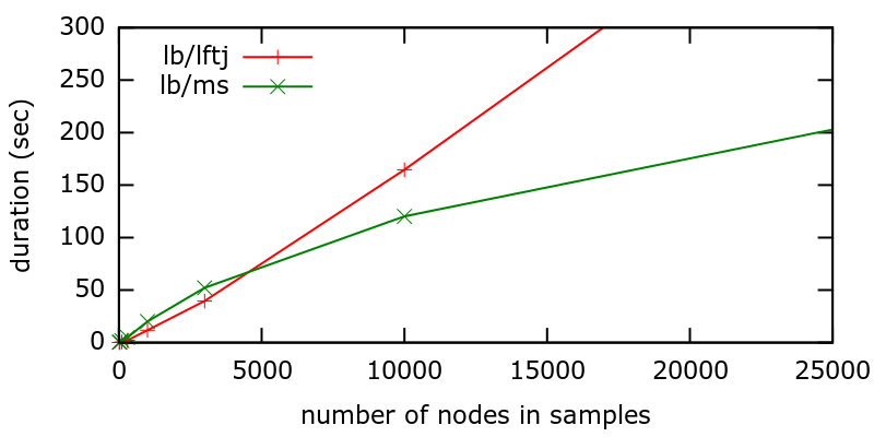
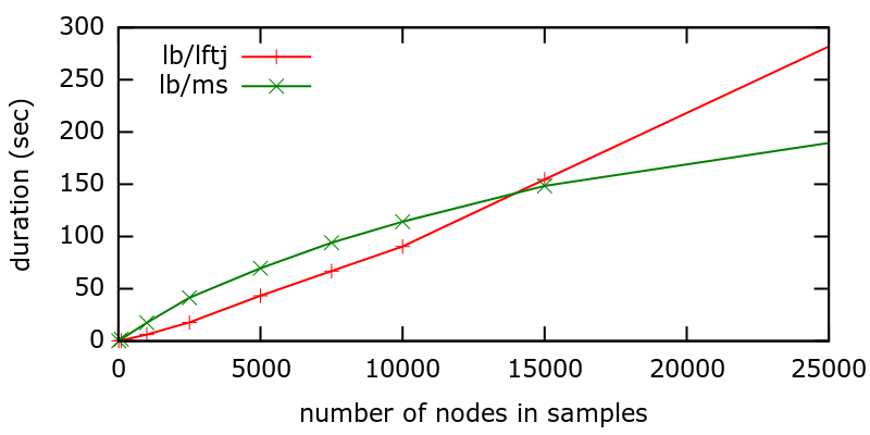
Figure 3: 3-path on LiveJournal with samples of N nodes

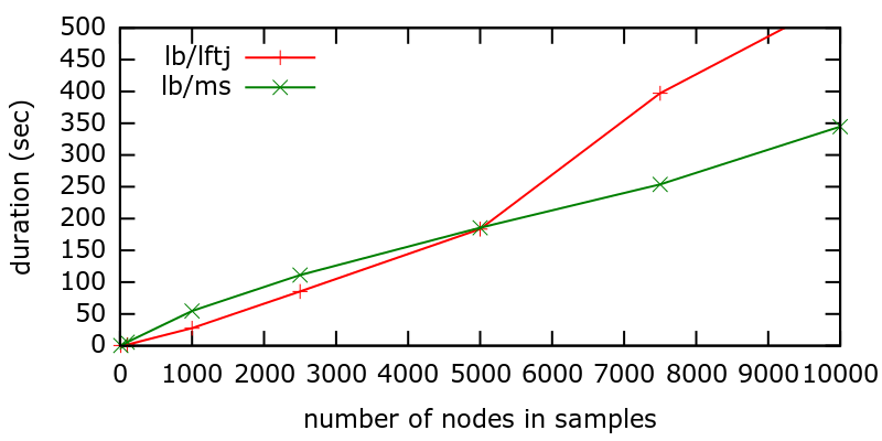
Figure 4: 3-path on Pokec with samples of N nodes

Figure 5: 3-path on Orkut with samples of N nodes

To illustrate the fact that Minesweeper has caching mechanism to avoid doing redundant work, Figure 5, 5, and 5 compare the performance of the algorithms when 3-path is executed with increasingly larger node samples.

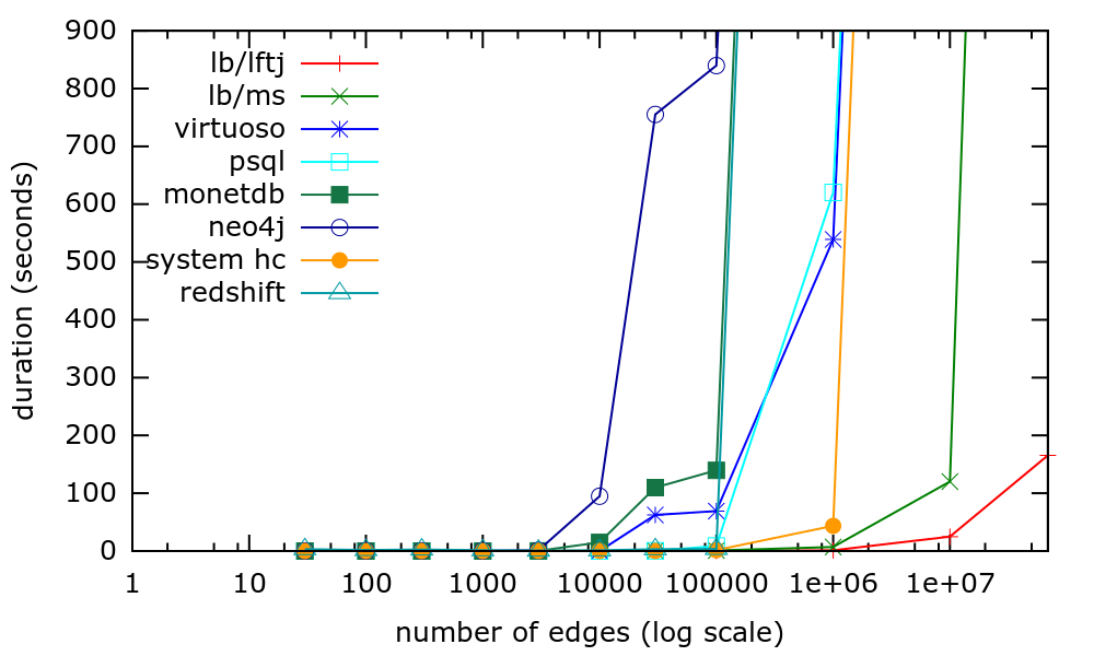
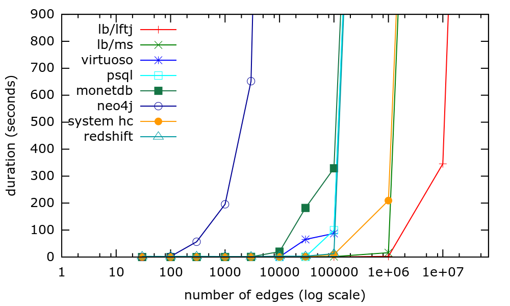
Figure 6: Duration of 3-clique on LiveJournal subset of N edges

Figure 7: Duration of 4-clique on LiveJournal subset of N edges

Scaling Behavior

To understand the scaling issues better, we eliminate the variability of the different datasets and execute a separate experiment where we gradually increase the number of edges selected from the LiveJournal dataset with a timeout of 15 minutes. This time we also include RedShift and System HC. The results are shown in Figures 7 and 7. This analysis shows that conventional relational databases (and Neo4J) do not handle this type of graph query even for very small data sets. Virtuoso is the best after the optimal joins. Optimal joins can handle subsets of two orders of magnitude bigger, and LFTJ supports an order of magnitude bigger graphs than Minesweeper.

Summary

LogicBlox using the LFTJ or Minesweeper algorithms consistently out-performs other systems that support high-level languages. LFTJ performs fastest on cyclic queries and is competitive on acyclic queries (1-tree) or queries with very high selectivity. Minesweeper works best for all other acyclic queries and performs particularly well for queries with low selectivity due to its caching.

6 Conclusion

Our results suggest that this new class of join algorithms allows a fully featured, SQL relational database to compete with (and often outperform) graph database engines for graph-pattern matching. One direction for future work is to extend this benchmark to recursive queries and more graph-style processing (e.g., BFS, shortest path, page rank). A second is to use this benchmark to refine this still nascent new join algorithms. In the full version of this paper, we propose and experiment with a novel hybrid algorithm between LFTJ and Minesweeper. We suspect that there are many optimizations possible for these new breed of algorithms.

Appendix A AGM bound

Given a join query $Q$ whose hypergraph is $\mathcal{H}(Q)=(\mathcal{V},\mathcal{E})$, we index the relations using edges from this hypergraph. Hence, instead of writing $R(\textnormal{vars}(R))$, we can write $R_{F}$, for $F\in\mathcal{E}$.

A fractional edge cover of a hypergraph $\mathcal{H}$ is a point $\mathbf{x}=(x_{F})_{F\in\mathcal{E}}$ in the following polyhedron:

$$\left\{\mathbf{x}\ |\ \sum_{F:v\in F}x_{F}\geq 1,\forall v\in\mathcal{V},\mathbf{x}\geq\mathbf{0}\right\}.$$

Atserias-Grohe-Marx [3] and Grohe-Marx [6] proved the following remarkable inequality, which shall be referred to as the AGM’s inequality. For any fractional edge cover $\mathbf{x}$ of the query’s hypergraph,

$$|Q|=|\Join_{F\in\mathcal{E}}R_{F}|\leq\prod_{F\in\mathcal{E}}|R_{F}|^{x_{F}}.$$ (3)

Here, $|Q|$ is the number of tuples in the (output) relation $Q$.

The optimal edge cover for the AGM bound depends on the relation sizes. To minimize the right hand side of (3), we can solve the following linear program:

$$\min \sum_{F\in\mathcal{E}}(\log_{2}|R_{F}|)\cdot x_{F}$$

s.t. $$\sum_{F:v\in F}x_{F}\geq 1,v\in\mathcal{V}$$

$$\mathbf{x}\geq\mathbf{0}$$

Implicitly, the objective function above depends on the database instance $\mathcal{D}$ on which the query is applied. We will use $\textsf{AGM}(Q)$ to denote the best AGM-bound for the input instance associated with $Q$. AGM showed that the upper bound is essentially tight in the sense that there is a family of database instances for which the output size is asymptotically the same as the upper bound. Hence, any algorithm whose runtime matches the AGM bound is optimal in the worst-case.

Appendix B Tuning parameters per system

tuning parameter		value
psql	temp_buffers	2GB
	work_mem	256MB
virtuoso	NumberOfBuffers	2380000
	MaxDirtyBuffers	1750000
	TransactionAfterImageLimit	99999999
neo4j	neostore.nodestore.db.mapped_memory	500M
	neostore.relationshipstore.db.mapped_memory	3G
	neostore.propertystore.db.mapped_memory	500M
	wrapper.java.initmemory (-Xms)	16384
	wrapper.java.maxmemory (-Xmx)	16384
	wrapper.java.additional.1	-Xss1m
graphlab	ncpus	8

References

- [1] C. Aberger, A. Nötzli, K. Olukotun, and C. Ré. EmptyHeaded: Boolean Algebra Based Graph Processing. ArXiv e-prints, Mar. 2015.
- [2] S. Abiteboul, R. Hull, and V. Vianu. Foundations of Databases. Addison-Wesley, 1995.
- [3] A. Atserias, M. Grohe, and D. Marx. Size bounds and query plans for relational joins. SIAM J. Comput., 42(4):1737–1767, 2013.
- [4] R. Fagin. Degrees of acyclicity for hypergraphs and relational database schemes. J. ACM, 30(3):514–550, 1983.
- [5] R. Fagin, A. Lotem, and M. Naor. Optimal aggregation algorithms for middleware. In PODS, 2001.
- [6] M. Grohe and D. Marx. Constraint solving via fractional edge covers. In SODA, pages 289–298. ACM Press, 2006.
- [7] J. Leskovec and A. Krevl. SNAP Datasets: Stanford large network dataset collection. http://snap.stanford.edu/data, June 2014.
- [8] H. Q. Ngo, D. T. Nguyen, C. Re, and A. Rudra. Beyond worst-case analysis for joins with Minesweeper. In PODS, pages 234–245, 2014.
- [9] H. Q. Ngo, E. Porat, C. Ré, and A. Rudra. Worst-case optimal join algorithms: [extended abstract]. In PODS, pages 37–48, 2012.
- [10] H. Q. Ngo, C. Ré, and A. Rudra. Skew strikes back: New developments in the theory of join algorithms. In SIGMOD RECORD, pages 5–16, 2013.
- [11] R. Ramakrishnan and J. Gehrke. Database Management Systems. McGraw-Hill, Inc., New York, NY, USA, 3 edition, 2003.
- [12] M. Rudolf, M. Paradies, C. Bornhövd, and W. Lehner. The graph story of the sap hana database. In BTW, 2013.
- [13] P. G. Selinger, M. M. Astrahan, D. D. Chamberlin, R. A. Lorie, and T. G. Price. Access path selection in a relational database management system. In SIGMOD, pages 23–34, New York, NY, USA, 1979. ACM.
- [14] T. L. Veldhuizen. Incremental maintenance for leapfrog triejoin. CoRR, abs/1303.5313, 2013.
- [15] T. L. Veldhuizen. Leapfrog triejoin: A simple, worst-case optimal join algorithm. In ICDT, pages 96–106, 2014.
- [16] T. L. Veldhuizen. Transaction repair: Full serializability without locks. CoRR, abs/1403.5645, 2014.
- [17] M. Yannakakis. Algorithms for acyclic database schemes. In VLDB, pages 82–94, 1981.