Local limit theorem in negative curvature

Abstract.

Consider the heat kernel $\wp(t,x,y)$ on the universal cover $\widetilde{M}$ of a closed Riemannian manifold of negative sectional curvature. We show the local limit theorem for $\wp$ :

$$\lim_{t\to\infty}t^{3/2}e^{\lambda_{0}t}\wp(t,x,y)=C(x,y),$$

where $\lambda_{0}$ is the bottom of the spectrum of the geometric Laplacian and $C(x,y)$ is a positive $\lambda_{0}$-harmonic function which depends on $x,y\in\widetilde{M}$.

We show that the $\lambda_{0}$-Martin boundary of $\widetilde{M}$ is equal to its topological boundary. The Martin decomposition of $C(x,y)$ gives a family of measures $\{\mu^{\lambda_{0}}_{x}\}$ on $\partial\widetilde{M}$. We show that $\{\mu^{\lambda_{0}}_{x}\}$ is a family minimizing the energy or the Rayleigh quotient of Mohsen.

We use the uniform Harnack inequality on the boundary $\partial\widetilde{M}$ and the uniform three-mixing of the geodesic flow on the unit tangent bundle $SM$ for suitable Gibbs-Margulis measures.

1. Introduction

Let $(M,d)$ be an $m$-dimensional closed connected Riemannian manifold of negative sectional curvature, and $(\widetilde{M},\widetilde{d})$ its universal cover endowed with the lifted Riemannian metric. Let us denote by $d$ the distance on $M$, $\widetilde{M}$, as well as on their unit tangent bundles $SM$ and $S\widetilde{M}$ (see [PPS] for various distances on $M$ and on $SM$ and the equivalences between them). Let us denote by $\pi:SM\to M$ and $\pi:S\widetilde{M}\to\widetilde{M}$ the projection of each vector to its base point and by ${p}\,$ the natural projection $(\widetilde{M},\widetilde{d})\to(M,d)$ and its derivative. The fundamental group $\Gamma=\pi_{1}(M)$ acts on $\widetilde{M}$ as isometries such that $M=\widetilde{M}/\Gamma$. Let $M_{0}$ be a bounded fundamental domain for this action.

We consider the geometric Laplace operator $\Delta:=-\mbox{Div}\nabla$ or smooth functions on $\widetilde{M}$ and the corresponding heat kernel function $\wp(t,x,y),t\in\mathbb{R}_{+},x,y\in\widetilde{M}$, which is the probability density defined as the fundamental solution of the heat equation, i.e. the function which satisfies $\frac{\partial\wp}{\partial t}+\Delta_{y}\wp=0$ and $\underset{t\to 0}{\lim}\;\wp(t,x,y)=\delta(x-y)$. The function $\wp$ is clearly $\Gamma$-invariant and symmetric in $x$ and $y$. See Section 8 for background on general potential theory and properties of the heat kernel.

Denote by $\lambda_{0}$ the bottom of the spectrum of the operator $\Delta$ on $L^{2}(\widetilde{M},\mbox{Vol})$, where $d\mbox{Vol}(z)$ is the Riemannian volume form on $\widetilde{M}$ (see Definition 8.1). Since $\Gamma$ is not amenable, $\lambda_{0}$ is positive [Br]. For all $x,y\in\widetilde{M}$, we have

(1.1) $$\lambda_{0}\;=\;\lim_{t\to\infty}-\frac{1}{t}\log\wp(t,x,y)$$

by the spectral theorem (See [CK] and [Sim]). Our main result is a local limit theorem which refines (1.1).

Theorem 1.1 (Local Limit Theorem).

There exists a positive function $C$ on $\widetilde{M}\times\widetilde{M}$ such that for all $x,y\in M$,

(1.2) $$\lim_{t\to\infty}t^{3/2}e^{\lambda_{0}t}\wp(t,x,y)\;=\;C(x,y).$$

When $\widetilde{M}$ is the hyperbolic space $\mathbb{H}^{3}$, there is an explicit expression for $\wp(t,x,y)$ ([DGM]) and Theorem 1.1 is clear, with

$$C(x,y)=(4\pi)^{-3/2}\frac{d(x,y)}{\sinh d(x,y)}.$$

In the case of symmetric spaces of non-compact type, i.e. when $\widetilde{M}=G/K$ for a semi-simple Lie group $G$ and a maximal compact subgroup $K$ of $G$, Bougerol proved an analog of Theorem 1.1 with $t^{k/2}$ instead of $t^{3/2}$, where the integer $k$ is given by the rank plus twice the number of positive indivisible roots. In particular, $k=3$ for all rank one symmetric spaces and this explains why one might expect $t^{3/2}$ for negatively curved manifolds. Bougerol proved the theorem for all random walks on $G$ with a distribution that is left and right $K$-invariant which implies the same result for Brownian motions on $\widetilde{M}$.

The limit function $C(x,y)$ is symmetric by Theorem 1.1 and it is a positive harmonic function in $y$ for the operator $(\Delta-\lambda_{0})$:

$$(\Delta-\lambda_{0})C(x,y)=0.$$

From now on, we will call such a harmonic function for $(\Delta-\lambda_{0})$ a $\lambda_{0}$-harmonic function. We further give a formula in Theorem 1.7 below. We remark that it was already known that if the limit

(1.3) $$\lim_{t\to\infty}\frac{\wp(t,x,y)}{\wp(t,x,x)}\;=\;\frac{C(x,y)}{C(x,x)}$$

exists on a Riemannian manifold, then $C(x,y)$ is a $\lambda_{0}$-harmonic function in $y$ [ABJ] (Theorem 1.2). It is indeed a conjecture by Davies ([Da]) that the limit (1.3) always exists (see [Ko] for a recent counterexample for the analogous question on graphs). Our result can be stated as:

Corollary 1.2.

The universal cover of a compact Riemannian manifold with negative sectional curvature satisfies Davies conjecture.

See [ABJ] for further discussion and applications of Davies conjecture.

A local limit theorem similar to Theorem 1.1 was first observed by Gerl [Ge] and Woess [GW] for random walks on a free group which are supported on a finite set of generators of the group. It was then proven by Lalley for random walks with finite support on a finitely generated free group [La]. This was extended by Gouëzel and Lalley to symmetric random walks with finite support on cocompact Fuchsian groups [GL] and finally by Gouëzel to symmetric random walks with finite support on hyperbolic groups [G1]. Our proof follows the strategy and ideas of [GL] and [G1]. By [G2], this general strategy works for measures of infinite support and with superexponential moments.

Two main new ingredients of the proof of Theorem 1.1 are the uniform rapid-mixing of the geodesic flow generalizing Dolgopyat theorem and the generalised Patterson-Sullivan conformal family whose Radon-Nikodym derivative is the Martin kernel $k^{2}_{\lambda_{0}}(x,y,\xi)$, which is defined in Theorem 1.4 below and which is a family realizing the minimum of Mohsen’s Rayleigh quotient (see Corollary 1.6).

As in [G1], we obtain several subsequent results which have their own interest. Let us introduce more notation to describe these results. For any real $\lambda<\lambda_{0}$, we define the $\lambda$-Green function $G_{\lambda}$: for all $x\not=y\in\widetilde{M}$,

$$G_{\lambda}(x,y)\;:=\;\int_{0}^{\infty}e^{\lambda t}\wp(t,x,y)dt.$$

The integral on the right hand side is finite: it converges at $\infty$ thanks to the spectral theorem (1.1) and it converges at 0 since as $t\to 0$, $\wp(t,x,y)\sim C/t^{m/2}e^{-\frac{d^{2}(x,y)}{4t}},$ which can be deduced from the fact that as $t\to 0$, the ambient space can be approximated by Euclidean space. The function $G_{\lambda}(x,\cdot)$ is positive and $\lambda$-harmonic for all $y\neq x$.

We first observe in Lemma 2.1 that for all $x\not=y\in\widetilde{M}$, the integral

$$G_{\lambda_{0}}(x,y)\;:=\int_{0}^{\infty}e^{\lambda_{0}t}\wp(t,x,y)dt$$

is finite. In Section 3, we show (see Proposition 3.12, where we relate $\tau$ with other dynamical properties)

Theorem 1.3.

There are positive constants $\tau$ and $C$ such that, for $x,y\in\widetilde{M}$ with $d(x,y)\geq 1,$

$$G_{\lambda_{0}}(x,y)\;\leq\;Ce^{-\tau d(x,y)}.$$

Two geodesic rays in $\widetilde{M}$ are said to be equivalent if they remain a bounded distance apart. The geometric boundary $\partial\widetilde{M}$ is defined as the space of equivalence classes of unit speed geodesic rays. A sequence $\{y_{n}\}_{n\in{\mathbb{N}}}$ in $\widetilde{M}$ converges to a point in $\partial\widetilde{M}$ if, and only if, for some (hence, for all) $x\in\widetilde{M}$,

$$d(x,y_{n})+d(x,y_{m})-d(y_{n},y_{m})\to\infty\quad{\textrm{as }}\;n,m\to\infty.$$

We now describe the Martin boundary of the operator $\Delta-\lambda_{0}$. The Martin boundary of $\Delta-\lambda_{0}$ is the closure of the embedding $y\to{k_{\lambda_{0}}}(\cdot,y)=\frac{{G_{\lambda_{0}}}(\cdot,y)}{G_{\lambda_{0}}(o,y)}$ in the space of functions with the topology of pointwise convergence. It is crucial for us to identify the Martin boundary of $\Delta-\lambda_{0}$ with the geometric boundary when we use thermodynamics formalism for the measures on the Martin boundary to obtain the Local Limit Theorem 1.1.

Theorem 1.4.

[$\lambda_{0}$-Martin boundary] Fix $x\in\widetilde{M}$ and assume that the sequence $\{y_{n}\}_{n\in{\mathbb{N}}}$ converges to a point $\xi\in\partial\widetilde{M}$. Then, there exist a positive $\lambda_{0}$-harmonic function $k_{\lambda_{0}}(x,y,\xi)$ of the Laplacian, which we call the Martin kernel, such that

$$\lim\limits_{n\to\infty}\frac{G_{\lambda_{0}}(y,y_{n})}{G_{\lambda_{0}}(x,y_{n})}\;=\;k_{\lambda_{0}}(x,y,\xi).$$

Moreover, the Martin boundary of $\Delta-\lambda_{0}$ coincides with the geometric boundary. In particular, for any positive $\lambda_{0}$-harmonic function $F$ and any $x\in\widetilde{M}$, there is a finite measure $\nu_{x,F}$ on $\partial\widetilde{M}$ such that

$$F(y)\;=\int_{\partial\widetilde{M}}k_{\lambda_{0}}(x,y,\xi)d\nu_{x,F}(\xi).$$

See Section 3 for the proof and more properties of the Martin kernel $k_{\lambda_{0}}(x,y,\xi)$. The Martin kernel squared $k_{\lambda_{0}}^{2}(x,y,\xi)$ plays the role of a conformal density for a family of measures on the boundary $\partial\widetilde{M}$.

Theorem 1.5.

There is a family $\{\mu_{x}^{\lambda_{0}}\}_{x\in\widetilde{M}}$ of finite measures on $\partial\widetilde{M}$ such that

• the family $x\mapsto\mu_{x}^{\lambda_{0}}$ is $\Gamma$-equivariant: $\mu_{\gamma x}^{\lambda_{0}}=\gamma_{\ast}(\mu_{x}^{\lambda_{0}})$ for $\gamma\in\Gamma$ and

• for $\mu_{x}^{\lambda_{0}}$-a.e. $\xi\in\partial\widetilde{M}$, all $y\in\widetilde{M}$, we have

  $$\frac{d\mu_{y}^{\lambda_{0}}}{d\mu_{x}^{\lambda_{0}}}(\xi)\;=\;k_{\lambda_{0}}^{2}(x,y,\xi).$$

The family is unique if we normalize by $\int_{M_{0}}\mu_{x}^{\lambda_{0}}(\partial\widetilde{M})d\mbox{Vol}(x)=1.$

Consider a $\Gamma$-equivariant family $\nu=\{\nu_{x}\}_{x\in\widetilde{M}}$ of measures on $\partial\widetilde{M}$ with cocycle $\ell(x,y,\xi):=\frac{d\nu_{y}}{d\nu_{x}}(\xi)$ and normalized by $\int_{M_{0}}\nu_{x}^{\lambda_{0}}(\partial\widetilde{M})d\mbox{Vol}(x)=1$. Assume that for $\nu$-a.e. $\xi$, the function $y\mapsto\log{\ell(x,y,\xi)}$ is a Lipschitz continuous function on $\widetilde{M}$ so that the value $\|\nabla_{y}\log{\ell(x,y,\xi)}\|$, which is independent of $x$, is defined for almost every $(x,y,\xi)$ . For such a family $\nu$, we define the energy of $\nu$ as follows:

$$\mathcal{E}(\nu):=\int_{M_{0}}\left(\int_{\partial\widetilde{M}}\|\nabla_{y=x}\log{\ell(x,y,\xi)}\|^{2}d\nu_{x}(\xi)\right)d\mbox{Vol}(x),$$

We define the energy to be infinite otherwise. Since for any fixed $x_{0},$

(1.4) $$\|\nabla|_{y=x}\log\ell(x_{0},y,\xi)\|^{2}=\frac{\|\nabla|_{y=x}\ell(x_{0},y,\xi)\|^{2}}{\ell^{2}(x_{0},x,\xi)}=4\|\nabla|_{y=x}\sqrt{\ell(x_{0},y,\xi)}\|^{2}\frac{d\nu_{x_{0}}}{d\nu_{x}},$$

the energy is equal to 4 times the Rayleigh quotient

$$\mathcal{R}(\nu):=\int_{M_{0}}\left(\int_{\partial\widetilde{M}}\|\nabla_{x}\sqrt{\ell(x_{0},x,\xi)}\|^{2}d\nu_{x_{0}}(\xi)\right)d\mbox{Vol}(x)$$

defined by O. Mohsen in [Mo]. Mohsen showed that $\lambda_{0}=\inf_{\nu}\mathcal{R}(\nu)$ and asked whether the minimum is achieved. We have

Corollary 1.6.

The family $\mu^{\lambda_{0}}_{x}$ achieves the minimum Rayleigh quotient.

See Section 5.2.3 for a proof. Mohsen proved the uniqueness for the manifolds with constant negative curvature.

The family $\mu^{\lambda_{0}}_{x}$ is a fourth natural $\Gamma$-equivariant family $\nu=\nu_{x}$ of measures on $\partial\widetilde{M}$ with regular cocycles, alongside with the Lebesgue visual measures, the Margulis-Patterson-Sullivan measures and the harmonic measures. Observe that the energy of the Margulis-Patterson-Sullivan measure is the volume entropy squared, and the energy of the harmonic measure is the Kaimanovich entropy [H2], [K1], [L3]. For rank one symmetric spaces, all of these families are the same up to normalization.

The last result we would like to emphasize is a formula of the function $C(x,y)$ in Theorem 1.1.

Theorem 1.7.

Fix $x\in\widetilde{M}$. There is a constant $\Upsilon=\Upsilon_{\lambda_{0}}$ such that the positive $\lambda_{0}$-harmonic function $C(x,y)$ satisfies

$$C(x,y)\;=\frac{\sqrt{\Upsilon}}{2\sqrt{\pi}}\int_{\partial\widetilde{M}}k_{\lambda_{0}}(x,y,\xi)d\mu^{\lambda_{0}}_{x}(\xi)\;=\;\frac{\sqrt{\Upsilon}}{2\sqrt{\pi}}\int_{\partial\widetilde{M}}\sqrt{d\mu^{\lambda_{0}}_{x}(\xi)}\sqrt{d\mu^{\lambda_{0}}_{y}(\xi)}.$$

Note that the formula for the constant $\Upsilon$ is given by (2.13).

Here, $\displaystyle\int_{\partial\widetilde{M}}\sqrt{d\mu^{\lambda_{0}}_{x}(\xi)}\sqrt{d\mu^{\lambda_{0}}_{y}(\xi)}:=\int_{\partial\widetilde{M}}\sqrt{\frac{d\mu_{y}^{\lambda_{0}}}{d\mu_{x}^{\lambda_{0}}}(\xi)}d\mu_{x}^{\lambda_{0}}(\xi)$ as used in unitary representation of $\Gamma$ associated to its action on $(\partial\widetilde{M},\mu^{\lambda_{0}}).$ In case of symmetric spaces, the function $C(x,y)$ is the positive $\lambda_{0}$-harmonic function invariant under the stabilizer $K_{x}$ of the point $x$, a.k.a. the Harish-Chandra function, or the ground state, centered at $x$.

The article is organized along the path of the proof of Theorem 1.1.

In Section 2, we recall the consequences of Ancona’s boundary Harnack inequality for $\lambda<\lambda_{0}$ ([An1]), in conjunction with the thermodynamic formalism for the geodesic flow (following [K1], [H3] and [L2]). Using mixing properties of the geodesic flow on the unit tangent bundle $SM$ for suitable $\Gamma$-invariant Gibbs measures, we show that there is a function $P(\lambda)$ of $\lambda$ and a positive function $D(x,\lambda)$ such that, for $\lambda<\lambda_{0}$, as $R\to\infty$

(1.5) $$e^{-P(\lambda)R}\int_{S(x,R)}G_{\lambda}^{2}(x,z)dz\to D(x,\lambda),$$

where $P(\lambda)<0$ for $\lambda<\lambda_{0}$ and $S(x,R)$ is the sphere of radius $R$ centered at $x$ (see Proposition 2.10).

We also recall from [H3] Corollary 5.5.1 that $\int_{S(x,R)}G_{\lambda_{0}}^{2}(x,z)dz$ is bounded independently of $R$ (Proposition 2.16).

In Section 3, we use this bound to establish the uniform Harnack inequality at the boundary, i.e. the Ancona-Gouëzel inequality (Theorem 3.2). Theorem 1.4 follows and the other applications of thermodynamic formalism hold equally at $\lambda=\lambda_{0}$.

In Section 4, we discuss limits of measures on large spheres using uniform mixing of the geodesic flow. One consequence of our results is that the measures $\mu_{x,R}$ on the spheres $S(x,R)$ with density $e^{-RP(\lambda_{0})}G^{2}_{\lambda_{0}}(x,y)$ converge to some measure $\mu^{\lambda_{0}}_{x}$ as $R\to\infty$ (Corollary 4.9). The measures $\mu^{\lambda_{0}}_{x}$ turn out to be a $\Gamma$-equivariant family with regular cocycle $e^{P(\lambda_{0})\beta(x,y,\xi)}k^{2}_{\lambda_{0}}(x,y,\xi)$, where $\beta(x,y,\xi)$ is the Busemann function (see the equation (2.9)). On the other hand, for $\lambda\in[0,\lambda_{0}],x\in\widetilde{M}$ and $R>2$, we define the measure $m_{x,\lambda,R}$ on $SM$ by:

lifting the measure $e^{-P({\lambda})R}G_{\lambda}^{2}(x,z)dz$ on $S(x,R)$ to the set

of unit vectors pointing towards $x$, then projecting to $SM$ by ${p}\,$.   ($*$)

Another consequence is that there exists a probability measure $\overline{m}$ over $SM$ such that the measures $m_{x,\lambda,R}$ converge towards $\mu^{\lambda_{0}}_{x}(\partial\widetilde{M})\overline{m}$ on $SM$ as $R\to\infty$ and $\lambda\to\lambda_{0}$ (see Corollary 4.10).

Once we prove that $P(\lambda_{0})=0$ in Section 5, the family of measures $\mu_{y}^{\lambda_{0}}$ satisfies the statements of Theorem 1.5. We also obtain that for $x,y\in\widetilde{M}$, $\displaystyle\lim\limits_{\lambda\to\lambda_{0}}-P({\lambda})\frac{\partial}{\partial\lambda}G_{\lambda}(x,y)$ is proportional to $C(x,y)$.

By a precise study of the second derivative $\displaystyle\frac{\partial^{2}}{\partial\lambda^{2}}G_{\lambda}(x,y)$ in Section 6.1, we obtain that both

$$\frac{P({\lambda})}{\sqrt{\lambda_{0}-\lambda}}{\textrm{ and }}\sqrt{\lambda_{0}-\lambda}\frac{\partial}{\partial\lambda}G_{\lambda}(x,y)$$

converge towards positive numbers as $\lambda\to\lambda_{0}.$ In Section 6.2, we conclude the proof of Theorem 1.1 from Theorem 6.1 thanks to a Tauberian Theorem as in [GL]. Theorem 1.7 follows as well.

In Section 7, we prove a uniform version of Dolgopyat’s rapid-mixing for hyperbolic flows which is an important tool for the proofs in the previous sections. As its proof is independent of the rest of the sections and the result is of independent interest as well, we made an Appendix for it. In Section 8, for completeness, we prove the precise balayage estimates in the form that is used in the article.

Remark 1.8.

In this text, $C$ stands for a number depending only on the geometry of $M$ and $\Gamma$. However, its actual value may change from one formula to another. For the sake of clarity, we specify $C_{0},\cdots,C_{11},C_{\varepsilon},C(T)$ when the same number is used in another computation. Note that $C_{1},C_{6},C_{7}$ in Section 7 have the same role as in [Me]. Likewise, we consider spaces of $\alpha$-Hölder continuous functions for some $\alpha$ of which the actual value may vary. Let us also remark that when the constant changes from one line to another, we used the symbols $\simeq$ and $\lesssim$ to indicate that the constant has changed.

Acknowledgement : We would like to thank M. Pollicott for generously sharing his insights and ideas [P1], [P2], P. Bougerol for his interest and the [ABJ] reference and S. Gouëzel for helpful comments. We are very grateful to several referees for their many precise and thoughtful remarks. The work was supported by University of Notre Dame, Seoul National University and MSRI during our visits. The second author was supported by NRF-2013R1A1A2011942, SSTF-BA1601-03 and Korea Institute for Advanced Study (KIAS).

2. Potential theory and thermodynamic formalism

We recall in this section the results obtained by applying classical potential theory to the Laplacian on $\widetilde{M}$ and thermodynamic formalism to the geodesic flow. See Section 8 for general potential theory. We have $G_{\lambda_{0}}(x,y)=\int_{0}^{\infty}e^{\lambda_{0}t}\wp(t,x,y)\,dt,$ where $\lambda_{0}$ is defined in Definition 8.1.

Lemma 2.1.

For any $x\neq y$,

(2.1) $$G_{\lambda_{0}}(x,y)<\infty.$$

For any $x$ and any compact set $K\subset\widetilde{M}$ with non-empty interior, we have

(2.2) $$\int_{K}G_{\lambda_{0}}(x,y)\,d\mathrm{Vol}(y) < \infty.$$

Proof.

The following argument is inspired by an idea of Guivarc’h in case of Lie groups. Let $\phi$ be a positive $\lambda_{0}$-harmonic function of the Laplacian, i.e. $\Delta\phi=\lambda_{0}\phi$, which exists by Lemma 8.2 (1). Then $q(t,x,y)$ defined in (8.2) defines a Markov process $D$ with its Green function $G_{D}(x,y)=G_{\lambda_{0}}(x,y)\frac{\phi(y)}{\phi(x)}.$

Suppose on the contrary to (2.2) that there is a compact set $K$ with non-empty interior such that $\int_{K}G_{\lambda_{0}}(x,y)\,d\mathrm{Vol}(y)=\infty$. It implies that $\int_{K}G_{D}(x,y)\,d\mathrm{Vol}(y)=\infty$. By the proof of Theorem 4.2.1.(ii) of [Pi], $G_{D}(x,y)=\infty$, which implies $G_{\lambda_{0}}(x,y)=\infty$, for all $y$. By Lemma 8.2 (2), there is a unique $\lambda_{0}$-harmonic function $\phi$ up to multiplicative constant. It follows that $\phi(y)/\phi(x)$ is $\Gamma$-invariant, thus $G_{D}$ is $\Gamma$-invariant. By discretization (see the proof of the main theorem of [BL]) there is a recurrent random walk $\mu_{D}$ on $\Gamma$ with Green function $G_{D}$, which implies that $\Gamma$ is virtually $\mathbb{Z},\mathbb{Z}^{2}$ or trivial [V], which is a contradiction. Thus $G_{\lambda_{0}}(x,y)<\infty$ for some $y\neq x$.

Equation (2.1) follows from Equation (2.2) since if $G_{\lambda_{0}}(x,y)<\infty$ at some points $y\not=x,$ then $G_{\lambda_{0}}(x,y)<\infty$ at all points $y\not=x$ (see [Da], Theorem 13). ∎

Proposition 2.2.

We have, for $\lambda\in[0,\lambda_{0})$, for any two points $x\not=y\in\widetilde{M}$:

(2.3) $$\frac{\partial^{k}}{\partial\lambda^{k}}G_{\lambda}(x,y)\;=\;k!\int_{\widetilde{M}^{k}}G_{\lambda}(x,x_{1})G_{\lambda}(x_{1},x_{2})\cdots G_{\lambda}(x_{k},y)\,d{\textrm{Vol}}^{k}(x_{1},\cdots,x_{k}).$$

Proof.

It follows from computation (see [GL] Proposition 1.9). For example, for $k=1$,

$$\int_{\widetilde{M}}G_{\lambda}(x,z)G_{\lambda}(z,y)dz =\int_{0}^{\infty}\int_{0}^{\infty}\int_{\widetilde{M}}e^{\lambda(t+u)}\wp(t,x,z)\wp(u,z,y)dzdtdu$$

$$\stackrel{{\scriptstyle(8.1)}}{{=}}\int_{0}^{\infty}\int_{0}^{\infty}e^{\lambda(t+u)}\wp(t+u,x,y)dtdu$$

$$=\int_{0}^{\infty}\int_{0}^{s}e^{\lambda s}\wp(s,x,y)dtds=\int_{0}^{\infty}se^{\lambda s}\wp(s,x,y)ds=\frac{\partial}{\partial\lambda}G_{\lambda}(x,y).$$

∎

Since the Green function is positive, by (2.3) for $k=1$ and $2$, the map $\lambda\mapsto G_{\lambda}(x,y)$ is a convex increasing function. Since $G_{\lambda}(x,y)$ is analytic outside the spectrum as a resolvent, its derivative is finite as well, i.e.

(2.4) $${\textrm{for all }}\lambda<\lambda_{0},\;{\textrm{ all }}x\not=y\in\widetilde{M},\;\int_{\widetilde{M}}G_{\lambda}(x,z)G_{\lambda}(z,y)d\mbox{Vol}(z)<+\infty.$$

For each $x\in\widetilde{M}$ and $v\in S_{x}\widetilde{M}$, let $\sigma_{x}(v)$ be the equivalence class of the geodesic $\gamma_{v}$ with the initial vector $v$. The mapping $\sigma_{x}$ is a homeomorphism from the unit tangent sphere $S_{x}\widetilde{M}$ of $\widetilde{M}$ at $x$ to $\partial\widetilde{M}$. Thus we will identify the unit tangent bundle $S\widetilde{M}$ with $\widetilde{M}\times\partial\widetilde{M}$.

For each $x\in\widetilde{M}$, $\partial\widetilde{M}$ is endowed with the Gromov metric

$$d_{x}(\xi,\eta)\;=\;e^{-a(\xi|\eta)_{x}},$$

where $0<a\leq 1$ is such that the sectional curvature $\kappa$ satisfies $\kappa\leq-a^{2}$ on $\widetilde{M}$ and $(\xi|\eta)_{x}$ is the Gromov product

(2.5) $$(\xi|\eta)_{x}=\lim\limits_{y\to\xi,z\to\eta}\frac{1}{2}\left(d(x,y)+d(x,z)-d(y,z)\right).$$

The following properties follow from pinched negative curvature:

Proposition 2.3 ([An1]).

For all $\lambda\in[0,\lambda_{0})$, every $\xi\in\partial\widetilde{M}$ there exist a positive $\lambda$-harmonic function $k_{\lambda}(x,y,\xi)$ in $y$ such that for each $x,y\in\widetilde{M},$

(2.6) $$\lim\limits_{z\to\xi}\frac{G_{\lambda}(y,z)}{G_{\lambda}(x,z)}\;=\;k_{\lambda}(x,y,\xi).$$

For any positive $\lambda$-harmonic function $F$, any $x\in\widetilde{M}$, there is a measure $\nu_{x,F}$ on $\partial\widetilde{M}$ such that

$$F(y)\;=\int_{\partial\widetilde{M}}k_{\lambda}(x,y,\xi)d\nu_{x,F}(\xi).$$

Proposition 2.4 ([H1]).

Moreover, for all $\lambda\in[0,\lambda_{0})$, there are constants $\alpha(\lambda)>0,C(\lambda)>0$ such that

$$\frac{\|\nabla_{y}\log k_{\lambda}(x,y,\xi)-\nabla_{y}\log k_{\lambda}(x,y,\eta)\|}{(d_{x}(\xi,\eta))^{\alpha(\lambda)}}\;\leq\;C(\lambda).$$

Proposition 2.5 ([K1]).

For three distinct points $x,y,z\in\widetilde{M}$, consider the function

(2.7) $$\theta_{x}^{\lambda}(y,z)\;:=\;\frac{G_{\lambda}(y,z)}{G_{\lambda}(y,x)G_{\lambda}(x,z)}.$$

There is a positive function $\theta_{x}^{\lambda}(\xi,\eta)$ on $\partial\widetilde{M}\times\partial\widetilde{M}\backslash\mathrm{Diag}:=\{(\xi,\eta)\in\partial\widetilde{M}\times\partial\widetilde{M}:\xi\neq\eta\}$ such that

$$\theta_{x}^{\lambda}(\xi,\eta)\;=\;\lim\limits_{y\to\xi,z\to\eta}\theta_{x}^{\lambda}(y,z).$$

The function $\theta_{x}^{\lambda}(\xi,\eta)$, when it is finite as it is here, is called the Naïm kernel in potential theory [N]. Compare with the definition of the Gromov product (2.5).

Consider $v\in SM.$ For a lift $\widetilde{v}$ in $S\widetilde{M}$, consider the geodesic $\gamma_{\widetilde{v}}(t)$ with initial tangent vector $\dot{\gamma_{\widetilde{v}}}(0)=\tilde{v}.$ We will denote $\widetilde{v}^{-}=\gamma_{\widetilde{v}}(-\infty)$ and $\widetilde{v}^{+}=\gamma_{\widetilde{v}}(+\infty)$. Set, for $v\in SM$,

(2.8) $$\theta_{\lambda}(v)\;:=\;\theta_{\gamma_{\widetilde{v}}(0)}^{\lambda}(\widetilde{v}^{+},\widetilde{v}^{-}),$$

where $\widetilde{v}$ is any lift of $v$. Observe that, by definition, $\theta_{\lambda}(v)=\theta_{\lambda}(-v).$

Fix $x\in\widetilde{M}$. For $\xi\in\partial\widetilde{M},y\in\widetilde{M}$, the Busemann function $\beta(x,y,\xi)$ is defined by

(2.9) $$\beta(x,y,\xi)\;=\;\lim\limits_{y_{n}\to\xi}\left(d(x,y_{n})-d(y,y_{n})\right).$$

Since $\widetilde{M}$ is the universal cover of a closed manifold of negative curvature, we also use the thermodynamic formalism of the geodesic flow as in [K1], [H1], [L2].

The geodesic flow $\mathbf{g}=\{\mathbf{g}_{t}\}_{t\in\mathbb{R}}$ is defined on the unit tangent bundles $SM$ and $S\widetilde{M}$. On $SM$, the geodesic flow is an Anosov flow. For a $\mathbf{g}$-invariant probability measure $m$ on $SM$, denote by $h_{m}(\mathbf{g})$ the measure-theoretic entropy of the time-1 map $\mathbf{g}_{1}$ with respect to $m$ (see e.g. [W]) . For any continuous function $\varphi$, define the topological pressure $P(\varphi)$ of $\varphi$ by

(2.10) $$P(\varphi)\;:=\;\sup_{m}\left(h_{m}(\mathbf{g})+\int_{SM}\varphi dm\right),$$

where the supremum is taken over all $\mathbf{g}$-invariant probability measures on $SM$.

For all $\lambda\in[0,\lambda_{0})$, the potential function associated to $\lambda$ is the function on $SM$ defined as

$$\varphi_{\lambda}(v):=-2\frac{d}{dt}\log k_{\lambda}(\gamma_{\widetilde{v}}(0),\gamma_{\widetilde{v}}(t),\widetilde{v}^{+})\Big{|}_{t=0}.$$

We set $P(\lambda):=P(\varphi_{\lambda})$ for $0\leq\lambda<\lambda_{0}.$

Definition 2.6.

Define $m_{\lambda}$ to be the unique equilibrium probability measure of $\varphi_{\lambda}$, which attains the supremum in (2.10).

The measure $m_{\lambda}$ is mixing for the geodesic flow $\mathbf{g}$ of $M$. The generalized family of Patterson-Sullivan measures associated to the potential function $\varphi_{\lambda}$, characterized by the following proposition, can be used to describe $m_{\lambda}$ as in (2.11).

Proposition 2.7 ([L2]).

Fix $\lambda\in[0,\lambda_{0})$. There is a family of finite measures $\{\mu_{y}^{\lambda}\}_{y\in\widetilde{M}}$ on $\partial\widetilde{M}$ all in the same measure class such that

• the family $y\mapsto\mu_{y}^{\lambda}$ is $\Gamma$-equivariant: $\mu_{\gamma y}^{\lambda}=\gamma_{\ast}(\mu_{y}^{\lambda})$ for $\gamma\in\Gamma$ and

• given any $x,y\in\widetilde{M}$, for $\mu_{x}^{\lambda}$-a.e. $\xi\in\partial\widetilde{M}$,

  $$\frac{d\mu_{y}^{\lambda}}{d\mu_{x}^{\lambda}}(\xi)\;=\;k_{\lambda}^{2}(x,y,\xi)e^{P(\lambda)\beta(x,y,\xi)}.$$

The family is unique if we normalize by setting $\int_{M_{0}}\mu_{y}^{\lambda}(\partial\widetilde{M})d\mbox{Vol}(y)=1.$

Corollary 2.8.

There exists a constant $C>0$, such that for all $\lambda\in[0,\lambda_{0})$, all $x\in\widetilde{M}$,

$$C^{-1}\leq\mu_{x}^{\lambda}(\partial\widetilde{M})\leq C.$$

Proof.

By Proposition 8.3 applied to $k_{\lambda}(x,y,\xi)$, for $x,y\in M_{0}$, $|\log k_{\lambda}^{2}(x,y,\xi)|$ are bounded. By Proposition 8.3 again, the function $\varphi_{\lambda}$ is bounded by $2\log C_{0}$. It follows that the pressure $P(\lambda)$ is bounded. Thus, the Radon-Nikodym derivatives $\frac{d\mu^{\lambda}_{x}}{d\mu^{\lambda}_{y}}$ are bounded for $x,y\in M_{0}$ uniformly in $\lambda$. Since the total measure is 1, the corollary follows. ∎

Fix $x_{0}\in\widetilde{M}$. By the Hopf parametrization, i.e. by associating $(v^{-},v^{+},\beta(x_{0},\gamma_{v}(0),v^{+}))$ to $v$, we identify $S\widetilde{M}$ with $(\partial\widetilde{M}\times\partial\widetilde{M}\backslash{\textrm{Diag}}(\partial\widetilde{M}))\times\mathbb{R}$, where ${\textrm{Diag}}(\partial\widetilde{M})$ is the diagonal embedding. Since $(\theta^{\lambda}_{x}(\xi,\eta))^{2}e^{2P(\lambda)(\xi|\eta)_{x}}d\mu_{x}(\xi)d\mu_{x}(\eta)$ is independent of $x$, we define a $\Gamma$-invariant, $\mathbf{g}_{t}$-invariant measure $\widetilde{m}_{\lambda}$ by

(2.11) $$d\widetilde{m}_{\lambda}(\xi,\eta,t)=\Omega_{\lambda}(\theta^{\lambda}_{x}(\xi,\eta))^{2}e^{2P(\lambda)(\xi|\eta)_{x}}d\mu^{\lambda}_{x}(\xi)\times d\mu^{\lambda}_{x}(\eta)\times dt$$

on $S\widetilde{M}$, which does not depend on $x.$ Here, $\Omega_{\lambda}$ is the normalizing constant chosen so that the measure $\widetilde{m}_{\lambda}$ is equal to the $\Gamma$-invariant lift of the probability measure $m_{\lambda}$ to $S\widetilde{M}$.

Remark 2.9.

Note that we have a symmetric measure thanks to the fact that our potential function $\varphi_{\lambda}$ is cohomologous to $\varphi_{\lambda}\circ\iota$ where $\iota$ is the flip map $v\mapsto-v$ (compare with asymmetric measure in [PPS] Section 3.7). Indeed, we can write, for $v\in SM,t>0,$

$$\int_{0}^{t}(\varphi_{\lambda}-\varphi_{\lambda}\circ\iota)(\mathbf{g}_{s}v)\,ds = \int_{0}^{t}\varphi_{\lambda}(\mathbf{g}_{s}v)\;ds-\int_{0}^{t}\varphi_{\lambda}(-\mathbf{g}_{s}v)\;ds$$

$$= \log k_{\lambda}^{-2}(\gamma_{v}(0),\gamma_{v}(t),\gamma_{v}(+\infty))-\log k_{\lambda}^{-2}(\gamma_{v}(t),\gamma_{v}(0),\gamma_{v}(-\infty))$$

$$= -2\lim\limits_{s,s^{\prime}\to\infty}\log\frac{G_{\lambda}(\gamma_{v}(t),\gamma_{v}(s))G_{\lambda}(\gamma_{v}(t),\gamma_{v}(-s^{\prime}))}{G_{\lambda}(\gamma_{v}(0),\gamma_{v}(s))G_{\lambda}(\gamma_{v}(0),\gamma_{v}(-s^{\prime}))}$$

$$= \log\theta_{\lambda}^{2}(\gamma_{v}(t))-\log\theta_{\lambda}^{2}(\gamma_{v}(0)).$$

Note the role of $\log\theta^{2}_{\lambda}$ and its occurrence in the formula (2.11).

We can also identify the orthogonal two frame bundle $S^{2}\widetilde{M}$ with the triples of pairwise distinct points in $\partial\widetilde{M}\times\partial\widetilde{M}\times\partial\widetilde{M}$ by associating $(v,w\in v^{\perp})$ to $(v^{+},v^{-},w^{+})$. The measure

(2.12) $$d\widetilde{\tau}^{\lambda}_{x}(\xi,\eta,\zeta):=\Upsilon_{\lambda}\theta^{\lambda}_{x}(\xi,\eta)\theta^{\lambda}_{x}(\eta,\zeta)\theta^{\lambda}_{x}(\zeta,\xi)e^{P(\lambda)\left((\xi|\eta)_{x}+(\eta|\zeta)_{x}+(\zeta|\xi)_{x}\right)}\,d\mu^{\lambda}_{x}(\xi)d\mu^{\lambda}_{x}(\eta)d\mu^{\lambda}_{x}(\zeta)$$

does not depend on $x$ and is $\Gamma$-invariant. Here $\Upsilon_{\lambda}$ is the normalizing constant chosen so that the measure $\widetilde{\tau}^{\lambda}=\widetilde{\tau}^{\lambda}_{x}$ is equal to the $\Gamma$-invariant lift of the probability measure $\tau^{\lambda}$ to $S^{2}\widetilde{M}:$ for any fundamental domain $M_{0}$ for $\Gamma$,

(2.13) $$\widetilde{\tau}^{\lambda}(S^{2}M_{0})=1.$$

Let us recall dynamical foliations of $S\widetilde{M}$ in order to define measures associated to $\mu^{\lambda}_{x}$. For every $v\in S\widetilde{M}$, define the strong stable manifold, strong unstable manifold, weak (or central) stable manifold and weak (or central) unstable manifold of $v$ as follows:

$$W^{ss}(v) = \{w\in S\widetilde{M}:\underset{t\to+\infty}{\lim}d(\mathbf{g}_{t}v,\mathbf{g}_{t}w)=0\},$$

$$W^{uu}(v) = \{w\in S\widetilde{M}:\underset{t\to-\infty}{\lim}d(\mathbf{g}_{t}v,\mathbf{g}_{t}w)=0\},$$

$$W^{cs}(v) = \{w\in S\widetilde{M}:\exists s,\underset{t\to+\infty}{\lim}d(\mathbf{g}_{t+s}v,\mathbf{g}_{t}w)=0\},$$

$$W^{cu}(v) = \{w\in S\widetilde{M}:\exists s,\underset{t\to-\infty}{\lim}d(\mathbf{g}_{t+s}v,\mathbf{g}_{t}w)=0\}.$$

Recall that the homeomorphism $\sigma_{x}:S_{x}\widetilde{M}\to\partial\widetilde{M}$ sends $v$ to $v^{+}$. More generally, on any manifold $T$ transversal to the foliation into $\widetilde{W}^{cs}$, the mapping $v\mapsto\sigma_{\pi v}v$ defines a local homeomorphism $\sigma:T\to\partial\widetilde{M}.$ For any family of measures $\{\nu_{x}\}_{x\in\partial\widetilde{M}}$ with continuous densities $\ell(x,y,\xi):=\frac{d\nu_{y}}{d\nu_{x}}(\xi)$, the measure on $T$ with density $\ell(x_{0},\pi v,\sigma(v))$ with respect to $(\sigma^{-1})_{\ast}\nu_{x_{0}}$ does not depend on $x_{0}$ (see [PPS] Section 3.9 for example). Using the generalized Patterson-Sullivan measures $\mu^{\lambda}_{x}$ obtained in Proposition 2.7, we can therefore define measures $\mu_{\lambda}^{uu}$ on any transversal $T$ by

$$d\mu^{uu}_{\lambda}(w):=k_{\lambda}^{2}(x_{0},\pi(w),w^{+})e^{P(\lambda)\beta(x_{0},\pi(w),w^{+})}d(\sigma^{-1})_{\ast}\mu^{\lambda}_{x_{0}}(w),$$

for $w\in T$. They have the property that for two transversals through $\sigma_{x}^{-1}(\xi)$ and $\sigma_{y}^{-1}(\xi)$, respectively, the Radon-Nikodym derivative $\rho_{\lambda}(\sigma_{x}^{-1}(\xi),\sigma^{-1}_{y}(\xi))$ of the holonomy from $\sigma_{x}^{-1}(\xi)$ to $\sigma_{y}^{-1}(\xi)$ along the leaf $\widetilde{M}\times\{\xi\}$ is given by

(2.14) $$\rho_{\lambda}(\sigma_{x}^{-1}(\xi),\sigma^{-1}_{y}(\xi))=k^{2}_{\lambda}(x,y,\xi)e^{P(\lambda)\beta(x,y,\xi)}.$$

Observe that moreover, the family $\mu^{uu}_{\lambda}$ is $\Gamma$-equivariant and therefore defines a family of measures on transversals to the foliation into $W^{cs}$ in $SM.$ Similarly, using the mapping $v\mapsto\sigma_{\pi v}(-v)$, one associates to $\mu^{\lambda}_{x},x\in\partial\widetilde{M}$ an equivariant family of measures on the transversals to the foliation into $W^{cu}$:

$$d\mu^{ss}_{\lambda}(w)=k_{\lambda}^{2}(x_{0},\pi w,w^{-})e^{P(\lambda)\beta(x_{0},\pi(w),w^{-})}d(-\circ\sigma^{-1})_{\ast}\mu^{\lambda}_{x_{0}}(w)$$

that satisfy the same holonomy equation

(2.15) $$\rho_{\lambda}(-\sigma_{x}^{-1}(\eta),-\sigma^{-1}_{y}(\eta))=k^{2}_{\lambda}(x,y,\eta)e^{P(\lambda)\beta(x,y,\eta)}.$$

Observe that $\mu^{uu}_{\lambda}$ on $S_{x}\widetilde{M}$ is $(\sigma^{-1}_{x})_{*}\mu^{\lambda}_{x}$; note that

(2.16) $$\frac{d\mu^{uu}_{\lambda}}{d(\mathbf{g}_{-t})_{*}\mu^{uu}_{\lambda}}(v)=e^{-tP(\lambda)}k_{\lambda}^{2}(\gamma_{\widetilde{v}}(t),\gamma_{\widetilde{v}}(0),\gamma_{\widetilde{v}}(\infty)),$$

and for any continuous functions $f$ and $h$ on $SM$,

(2.17) $$\int_{S_{{p}x}M}f(v)\,d\mu_{\lambda}^{uu}(v) = \int_{\partial\widetilde{M}}f({p}\circ\sigma^{-1}_{x}\xi)d\mu_{x}^{\lambda_{0}}(\xi),$$

(2.18) $$\int_{S_{{p}y}M}h(-u)\,d\mu_{\lambda}^{ss}(u) = \int_{\partial\widetilde{M}}h({p}\,\circ\sigma^{-1}_{y}\xi)d\mu_{y}^{\lambda_{0}}(\xi),$$

By a direct generalization of Margulis argument [M1] to Gibbs measures, one obtains the following proposition (see Section 4 for details).

Proposition 2.10.

There exists a positive continuous function $D:(\widetilde{M}\times[0,\lambda_{0}))\to\mathbb{R}_{+}$ such that

$$\lim\limits_{R\to\infty}e^{-RP(\lambda)}\int_{S(x,R)}G_{\lambda}^{2}(x,z)dz\;=\;D(x,\lambda).$$

Clearly, $x\mapsto D(x,\lambda)$ is $\Gamma$-invariant and depends only on ${p}(x)\in M.$ The function $D(x,\lambda)$ will be described in Corollary 4.11.

Corollary 2.11.

For all $\lambda\in[0,\lambda_{0})$, we have $P(\lambda)<0.$

Proof.

Indeed, otherwise, we have by Proposition 8.3 and Proposition 2.10,

$$\int_{\widetilde{M}}G_{\lambda}(x,z)G_{\lambda}(z,y)d\mbox{Vol}(z)\gtrsim\int_{1+d(x,y)}^{+\infty}\left(\int_{S(x,R)}G_{\lambda}^{2}(x,z)dz\right)dR\gtrsim D(x,\lambda)\int_{1+d(x,y)}^{+\infty}dR.$$

The integral diverges, which is in contradiction with (2.4) for any $x\neq y$. ∎

The rest of this section is devoted to the proof of Proposition 2.16, originally due to Hamenstädt, and of Corollary 2.17. Firstly we observe that the easy side of the Ancona inequality is uniform in $\lambda\in[0,\lambda_{0}]$. For later use, we state this relation for the relative Green function $G_{\lambda}(x,y:\mathcal{D})$ associated to an open set $\mathcal{D}$ (see equation (8.3) for definition). If $\mathcal{D}=\widetilde{M},$ then $G_{\lambda}(x,y:\widetilde{M})=G_{\lambda}(x,y).$

Proposition 2.12.

There is a constant $C^{\prime}_{0}$ such that for any open set $\mathcal{D}$, any $0\leq\lambda\leq\lambda_{0}$ and any $x,y,z\in\mathcal{D}$ such that $d(x,z),d(x,y),d(x,\partial\mathcal{D}),d(y,\partial\mathcal{D}),d(z,\partial\mathcal{D})$ are all at least 1, we have

(2.19) $$G_{\lambda}(x,z:\mathcal{D})G_{\lambda}(x,y:\mathcal{D})\leq C^{\prime}_{0}G_{\lambda}(z,y:\mathcal{D}).$$

Proof.

By Corollary 8.5 for $0\leq\lambda\leq\lambda_{0}$ and $x,y,z$ such that $d(x,z),d(x,y),d(x,\partial\mathcal{D}),$ $d(y,\partial\mathcal{D}),d(z,\partial\mathcal{D})$ are all at least 1, we have

$$G_{\lambda}(x,z:\mathcal{D})G_{\lambda}(x,y:\mathcal{D})\leq C_{0}\max\{G_{\lambda}(x,y:\mathcal{D});d(x,y)\geq 1\}G_{\lambda}(z,y:\mathcal{D}).$$

For a fixed $\lambda<\lambda_{0}$, $G_{\lambda}(x,y:\mathcal{D})\leq G_{\lambda}(x,y)$ goes to 0 as $d(x,y)\to\infty$ (see[An1], Remark 2.1 page 505). By the maximum principle,

$$\max\{G_{\lambda}(x,y);d(x,y)\geq 1\}=\max\{G_{\lambda}(x,y);d(x,y)=1\}.$$

Moreover, $\max\{G_{\lambda}(x,y);d(x,y)=1\}\leq\max\{G_{\lambda_{0}}(x,y);d(x,y)=1\}.$ Set

$$C^{\prime}_{0}:=C_{0}\max\{G_{\lambda_{0}}(x,y);d(x,y)=1\}$$

which is finite by compactness. Relation (2.19) holds for all $\lambda<\lambda_{0}$, thus for $\lambda_{0}$ as well. ∎

Corollary 2.13.

For $0\leq\lambda<\lambda_{0}$, $x,z$ such that $d(x,z)\geq 1$ and $\xi\in\partial\widetilde{M}$, we have

(2.20) $$G_{\lambda}(x,z)\leq C^{\prime}_{0}k_{\lambda}(x,z,\xi).$$

Proof.

Divide the relation (2.19) by $G_{\lambda}(x,y)$ and let $y\to\xi$.∎

Two submanifolds $A,B$ of $S\widetilde{M}$ are said to be $\varepsilon$-transversal at an intersection point $x$ if the angle between the spaces $T_{x}A$ and $T_{x}B$ is greater than $\varepsilon$, and transversal if the angle is positive. If $\mathcal{W}$ is a lamination of $S\widetilde{M}$ with smooth leaves $W(x),x\in S\widetilde{M}$, $A$ is said to be $\varepsilon$-transversal to $\mathcal{W}$ if at each $x\in A$, $A$ and $W(x)$ are $\varepsilon$-transversal. For example, by the Anosov property, the unit sphere $S_{x}\widetilde{M}$ at $x$ and its images by the geodesic flow $\mathbf{g}_{t}$ for $t\geq 0$, are all $\varepsilon_{0}$-transversal to the central stable foliation $\mathcal{W}^{cs}$, for some $\varepsilon_{0}$.

Proposition 2.14.

Assume $A$ is $(m-1)$-dimensional and $\varepsilon$-transversal to $\mathcal{W}^{cs}$ and let $\delta>0$. There exists $R=R(\varepsilon,\delta)$ such that for any ball $B_{A}(x,\delta)\subset A,$

$$p\left(\cup_{x\in B_{A}(x,\delta)}B^{cs}(z,R)\right)\;=SM.$$

Proof.

It suffices to prove it for spheres. Consider the open set

$$V_{R}=\{(x,z)\in SM\times SM:B^{cs}(z,R)\cap B^{S}(x,\delta)\neq\emptyset\},$$

where $S=S_{p(x)}(M)$. By minimality of $\mathcal{W}^{cs}$ and the transversality of $S$ to $\mathcal{W}^{cs}$, we have $\underset{R>0}{\cup}V_{R}=SM\times SM.$ Therefore, $V_{R_{0}}=SM\times SM$ for some $R_{0}=R(\delta).$ It follows that for any $(x,z),$ there exists $y\in B^{cs}(z,R_{0})\cap B^{S}(x,\delta),$ i.e. $z\in B^{cs}(y,R_{0})$ for some $y\in B^{S}(x,\delta).$ ∎

If $A_{1},A_{2}$ are two $(m-1)$-dimensional submanifolds both transversal to $\mathcal{W}^{cs}$ and $x_{1}\in A_{1},x_{2}\in A_{2}$ belong to the same leaf $W^{cs}$ of $\mathcal{W}^{cs}$, then the holonomy from a neighborhood $B_{A_{1}}(x_{1})$ of $x_{1}$ in $A_{1}$, to a neighborhood $B_{A_{2}}(x_{2})$ of $x_{2}$ in $A_{2}$ is defined by continuously extending the intersection mapping which sends $x_{1}$ to $x_{2}$.

We defined above for $0\leq\lambda<\lambda_{0}$ a family of measures $\mu_{\lambda}^{uu}$ on $m-1$ dimensional transversals to $W^{cs}$ that are quasi invariant under the holonomy with Radon-Nykodym derivative

$$\rho_{\lambda}(\sigma_{x}^{-1}(\xi),\sigma^{-1}_{y}(\xi))=k^{2}_{\lambda}(x,y,\xi)e^{P(\lambda)\beta(x,y,\xi)}$$

and that coincide with $(\sigma^{-1}_{x})_{*}\mu^{\lambda}_{x}$ on $S_{x}\widetilde{M}.$

Corollary 2.15.

Let $A$ be a $(m-1)$-dimensional submanifold of $S\widetilde{M}$, $\varepsilon$-transversal to $\mathcal{W}^{s}$ and a ball $B_{A}(w,\delta)\subset A.$ There is a constant $C=C(\varepsilon,\delta)$ such that, for $0\leq\lambda<\lambda_{0},$

$$\mu_{\lambda}^{uu}(B(w,\delta))\;\geq\;C^{-1}.$$

Proof.

By Lemma  2.14, there is $R=R(\varepsilon,\delta)$ such that

$$p\left(\cup_{x\in B(w,\delta)}B^{cs}(x,R)\right)\;=SM.$$

In particular any sphere $S_{y}M$ is covered by $K$ holonomy images of $B(w,\delta),$ with $K$ bounded by some $K_{0}(\varepsilon,\delta)$. There is $C_{0}(\varepsilon,\delta)$ such that the Radon-Nykodym derivative of the measure $\mu_{\lambda}^{uu}$ under these holonomies are bounded by $C_{0}(\varepsilon,\delta)$. Therefore, for all $y\in M$, $\mu_{\lambda}^{uu}(S_{y}M)\leq K_{0}(\varepsilon,\delta)C_{0}(\varepsilon,\delta)\mu_{\lambda}^{uu}(B(w,\delta)).$ By our choice of normalisation, $\int_{M}\mu_{\lambda}^{uu}(S_{y}M)\,d\mathrm{Vol}(y)\;=\;1.$ Corollary 2.15 follows with $C=K_{0}(\varepsilon,\delta)C_{0}(\varepsilon,\delta)\mathrm{Vol}(M).$ ∎

The following proposition corresponds to [G1], Lemma 2.5.

Proposition 2.16 ([H3], Corollary 5.5.1)).

There is a constant $C>0$ such that for all $x\in\widetilde{M}$ and all $R\geq 1$,

$$\int_{S(x,R)}G_{\lambda_{0}}^{2}(x,z)dz\leq C.$$

Proof.

We first lift $S(x,R)\subset\widetilde{M}$ to $\mathbf{g}_{R}S_{x}\widetilde{M}\subset S\widetilde{M}.$ Let $w\in\mathbf{g}_{R}S_{x}\widetilde{M}$ and consider the ball $B(w,1)$ of radius 1 in $\mathbf{g}_{R}S_{x}\widetilde{M}$. The $(m-1)$-dimensional volume of $B(w,1)$ is bounded from above, uniformly in $R\geq 1$ and $w$, whereas by Corollary 2.15, $\mu_{\lambda}^{uu}(B(w,1))$ is bounded from below, uniformly in $\lambda,0\leq\lambda<\lambda_{0}.$ Finally, by Proposition 8.3, the function $G_{\lambda}^{2}(x,z)$ has a bounded oscillation on that set, uniformly in $\lambda,0\leq\lambda\leq\lambda_{0}.$ It follows that there is a constant $C$ such that for any $R\geq 1$, $0\leq\lambda<\lambda_{0}$ and a ball $B(w,1)$ of radius 1 in $\mathbf{g}_{R}S_{x}\widetilde{M}$,

$$\int_{B(w,1)}G^{2}_{\lambda}(x,\pi v)e^{-P(\lambda)R}dv\;\leq\;C\int_{B(w,1)}G^{2}_{\lambda}(x,\pi v)e^{-P(\lambda)R}\,d\mu_{\lambda}^{uu}(v).$$

By (2.20) and (2.16),

$$G^{2}_{\lambda}(x,\pi v)e^{-P(\lambda)R}\leq C^{\prime}_{0}k_{\lambda}^{2}(\pi v,x,\gamma_{v}(+\infty))e^{P(\lambda)\beta(\pi v,x,\gamma_{v}(+\infty))}=C^{\prime}_{0}\frac{d\mathbf{g}_{R}\mu^{uu}_{\lambda}}{d\mu^{uu}_{\lambda}}(v).$$

Altogether, we get, for any ball of radius 1 in $\mathbf{g}_{R}S_{x}\widetilde{M}$, for $0\leq\lambda<\lambda_{0},$

$$\int_{B(w,1)}G^{2}_{\lambda}(x,\pi v)e^{-P(\lambda)R}dv\leq CC^{\prime}_{0}\int_{B(w,1)}\frac{d\mathbf{g}_{R}\mu^{uu}_{\lambda}}{d\mu^{uu}_{\lambda}}(v)\,d\mu_{\lambda}^{uu}(v)=CC^{\prime}_{0}\mu_{\lambda}^{uu}(\mathbf{g}_{-R}(B(w,1))).$$

The sets $\mathbf{g}_{R}S_{x}\widetilde{M},R\geq 1$ are locally uniformly Lipschitz homeomorphic to open subsets of Euclidean $\mathbb{R}^{n-1}.$ Therefore we obtain a Besicovitch cover, i.e. there is an integer $N$, independent of $R$, and covers of $\mathbf{g}_{R}S_{x}\widetilde{M}$ by balls of radius 1 such that any point can belong to at most $N$ distinct balls. The images of the balls in that cover by $\mathbf{g}_{-R}$ form a cover of $S_{x}\widetilde{M}$ such that any point can belong to at most $N$ such images. Thus,

$$\int_{\mathbf{g}_{R}S_{x}\widetilde{M}}G^{2}_{\lambda}(x,\pi v)e^{-P(\lambda)R}dv\;\leq\;NCC^{\prime}_{0}\mu_{\lambda}^{uu}(S_{x}\widetilde{M}).$$

Since $\mu_{\lambda}^{uu}(S_{x}\widetilde{M})=\mu_{x}^{\lambda}(\partial\widetilde{M})$ is bounded by Corollary 2.8, we found a constant $C$ such that for all $\lambda<\lambda_{0}$ and for $R\geq 1,$

(2.21) $$\int_{S(x,R)}G^{2}_{\lambda}(x,z)e^{-P(\lambda)R}dz\leq C.$$

Here, we used the fact that the measures $\pi_{\ast}dv$, the projection of the Lebesgue measure for the restriction of the Sasaki metric to $\mathbf{g}_{R}S_{x}\widetilde{M}$, and $dz$, the Lebesgue measure on $S(x,R),$ are equivalent with bounded density.

Since $P(\lambda)<0$ for all $\lambda<\lambda_{0}$ by Corollary 2.11, there is a constant $C>0$ such that for all $\lambda\in[0,\lambda_{0})$, all $x\in\widetilde{M}$, all $R\geq 1$,

$$\int_{S(x,R)}G_{\lambda}^{2}(x,z)dz\leq C.$$

Proposition 2.16 follows by letting $\lambda$ go to $\lambda_{0}$. ∎

Corollary 2.17.

For $T>0$, let $P_{T}(\lambda)$ be the pressure of the function $\frac{T}{2}\varphi_{\lambda}$. Then there exists a constant $C(T)$ such that for all $\lambda\in[0,\lambda_{0}),R\geq 1,x\in\widetilde{M}$,

$$e^{-RP_{T}(\lambda)}\int_{S(x,R)}G_{\lambda}^{T}(x,z)dz\;\leq C(T).$$

Proof.

We have as above

$$G^{T}_{\lambda}(x,z)e^{-P_{T}(\lambda)d(x,z)}\leq{C_{0}^{\prime}}^{T}k^{T}_{\lambda}(x,z,\xi)e^{-P_{T}(\lambda)d(x,z)}.$$

We can also apply Proposition 2.7 to the Hölder continuous function $\frac{T}{2}\varphi_{\lambda}$ instead of $\varphi_{\lambda}$. We obtain a family of measures $\mu_{x}^{\lambda,T}$ on $\partial\widetilde{M}$ such that for all $\lambda\in[0,\lambda_{0})$, $\mu_{x}^{\lambda,T}$-a.e. $\xi\in\partial\widetilde{M}$,

$$\frac{d\mu_{y}^{\lambda,T}}{d\mu_{x}^{\lambda,T}}(\xi)\;=\;k_{\lambda}^{T}(x,y,\xi)e^{P_{T}(\lambda)\beta(x,y,\xi)}$$

and $\int_{M_{0}}\mu_{y}^{\lambda,T}(\partial\widetilde{M})d\mathrm{Vol}(y)=1.$ We can therefore associate measures $\mu^{uu}_{\lambda,T}$ on transversals to the central stable manifolds such that the holonomy from $\sigma_{x}^{-1}(\xi)$ to $\sigma_{y}^{-1}(\xi)$ along the leaf $\widetilde{M}\times\{\xi\}$ is given by

$$\rho_{\lambda}(\sigma_{x}^{-1}(\xi),\sigma^{-1}_{y}(\xi))=k^{T}_{\lambda}(x,y,\xi)e^{P_{T}(\lambda)\beta(x,y,\xi)}.$$

The same computation yields the analog of (2.21). ∎

3. Ancona-Gouëzel inequality

Definition 3.1.

Let $v\in S\widetilde{M}$. The cone $\mathcal{C}(v)$ based on $v$ is defined by:

$$\mathcal{C}(v)\;:=\;\{y;y\in\widetilde{M},\angle_{x}(v,y)\leq\pi/2\},$$

where $\angle_{x}(v,y)$ denotes the angle between $v\in T_{x}\widetilde{M}$ and the geodesic going from $x$ to $y$.

We denote $\partial\mathcal{C}(v):=\{y;y\in\widetilde{M},\angle_{x}(v,y)=\pi/2\}.$ Observe that $\widetilde{M}=\mathcal{C}(v)\cup\mathcal{C}(-v)$ and $\partial\mathcal{C}(v)=\mathcal{C}(v)\cap\mathcal{C}(-v).$

3.1. Ancona-Gouëzel inequality

The key property of the $\lambda$-Green functions for $0\leq\lambda\leq\lambda_{0}$ is the following uniform Ancona inequality, which we call Ancona-Gouëzel inequality. Recall the definition (8.3) of the relative Green function $G_{\lambda}(x,y:\mathcal{D})$, where $\mathcal{D}$ is an open subset of $\widetilde{M}$ and $x\neq y\in\mathcal{D}.$

Theorem 3.2.

There are constants $C_{4},R_{0}$ such that for all $\lambda\in[0,\lambda_{0}]$, all points $(x,y,z)$ such that $y$ is on the geodesic segment $[xz]$ from $x$ to $z$ and $d(x,y)\geq R_{0},d(y,z)\geq R_{0}$,

(3.1) $$C_{4}^{-1}G_{\lambda}(x,y:\mathcal{D})G_{\lambda}(y,z:\mathcal{D})\;\leq\;G_{\lambda}(x,z:\mathcal{D})\;\leq\;C_{4}G_{\lambda}(x,y:\mathcal{D})G_{\lambda}(y,z:\mathcal{D})$$

for all open sets $\mathcal{D}$ containing $\mathcal{C}(\mathbf{g}_{-1}v)\cap\mathcal{C}(-\mathbf{g}_{d(x,z)+1}v),$ where $v\in S_{x}\widetilde{M}$ is the initial vector of the geodesic $[xz]$.

Theorem 3.2 was proven by A. Ancona for $\lambda<\lambda_{0}$ ([An1]). The first inequality in (3.1) is uniform for $\lambda\in[0,\lambda_{0}]$ (see (2.19)). The new fact here is that the second inequality (3.1) holds when $\lambda=\lambda_{0}$ as well, with the same constant $C_{4}$, so that the consequences of Theorem 3.2 are now uniform in $\lambda\in[0,\lambda_{0}]$. The Ancona inequality follows from the pre-Ancona inequality in the following Proposition.

Proposition 3.3.

Let $x,y,z$ be points on a geodesic $\gamma$ in this order, $v$ the tangent vector to $\gamma$ at $x$. Then, there exists $\varepsilon>0,R_{2}>1$ such that if $r\geq R_{2}$ and $d(x,y)>r+1,d(y,z)>r+1,$ we have

$$G_{\lambda_{0}}(x,z:B(y,r)^{c}\cap\mathcal{C}(g_{-1}v)\cap\mathcal{C}(-\mathbf{g}_{d(x,z)+1}v))\leq 2^{-e^{\varepsilon r}}.$$

Proof.

As in [G1], we will construct $N=e^{\varepsilon r}$ barriers, for a positive constant $\varepsilon$ which we will specify as follows.

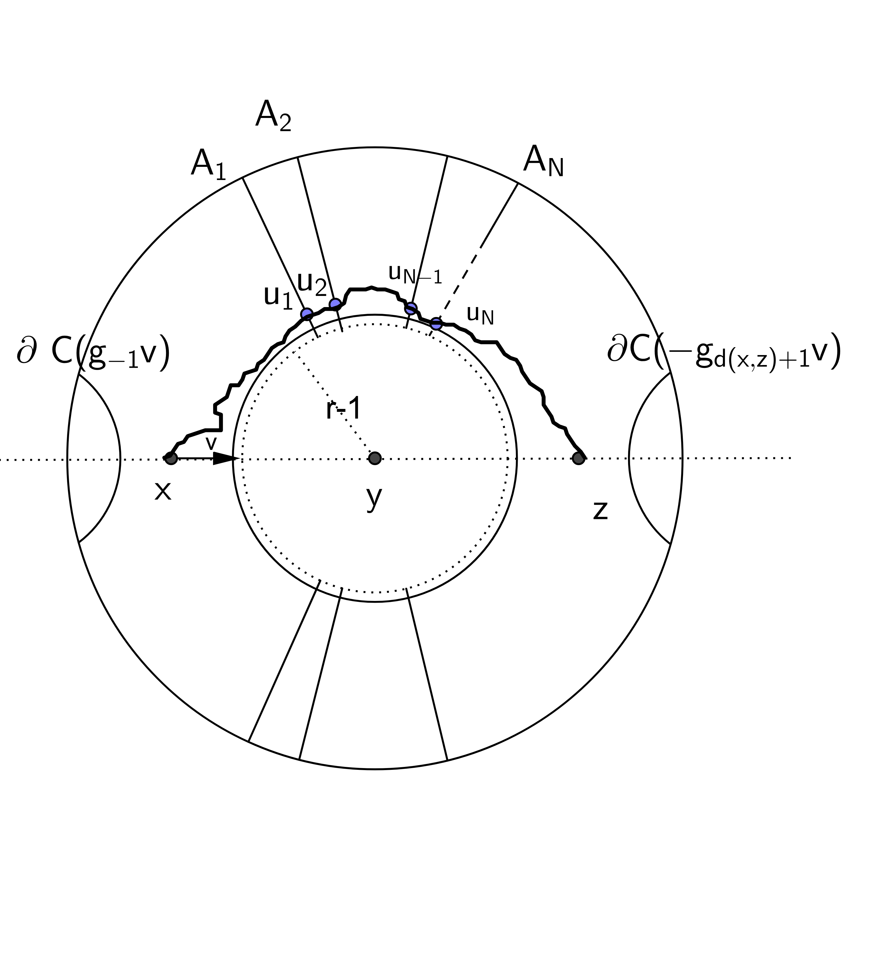
Figure 1. Ancona-Gouëzel inequality

For $i=1,\cdots,N$, let $X_{i}=((N+2i-1)\pi/4N,(N+2i)\pi/4N)\subset[\pi/4,3\pi/4]$. Choose $\theta_{i}$ from $X_{i}$, for $i=1,\cdots,N$.

By negative curvature, the intersections $\{A_{i}\}$’s of $B(y,r-1)^{c}$ and the cones $\{w:\angle_{y}(x,w)=\theta_{i}\}$ of angle $\theta_{i}$ at $y$, are of distance between them bounded below by $1$ for all $r$ large enough. Set $\mathcal{D}:=B(y,r)^{c}\cap\mathcal{C}(\mathbf{g}_{-1}v)\cap\mathcal{C}(-\mathbf{g}_{d(x,z)+1}v)$. Each set $A_{i}\cap\mathcal{D}$ separate $\mathcal{D}$ into two disjoint open sets. Let $\mathcal{C}_{i}$ be the one containing $x$. Then $z\not\in\mathcal{C}_{i}$. Moreover, the sets $A_{i}\cap\mathcal{D}$ have bounded geometry and do not intersect $\partial\mathcal{C}(\mathbf{g}_{-1}v)\cup\mathcal{C}(-\mathbf{g}_{d(x,z)+1}v)$ (see Figure 1).

By (8.6), we may write:

$$G_{\lambda_{0}}(x,z:\mathcal{D}) = \int_{A_{1}\cap\mathcal{D}}G_{\lambda_{0}}(u_{1},z:\mathcal{D})\,d\varpi_{x}^{\lambda_{0}}(u_{1})$$

$$= \int_{A_{1}\cap\mathcal{D}}\int_{A_{2}\cap\mathcal{D}}G_{\lambda_{0}}(u_{2},z:\mathcal{D})\,d\varpi_{x}^{\lambda_{0}}(u_{1})d\varpi_{u_{1}}^{\lambda_{0}}(u_{2})$$

$$= \int_{A_{1}\cap\mathcal{D}}\cdots\int_{A_{N}\cap\mathcal{D}}G_{\lambda_{0}}(u_{N},z:\mathcal{D})\,d\varpi_{x}^{\lambda_{0}}(u_{1})\cdots d\varpi_{u_{N-1}}^{\lambda_{0}}(u_{N})$$

$$\leq \int_{A_{1}\cap\mathcal{D}}\cdots\int_{A_{N}\cap\mathcal{D}}G_{\lambda_{0}}(u_{N},z)\,d\varpi_{x}^{\lambda_{0}}(u_{1})\cdots d\varpi_{u_{N-1}}^{\lambda_{0}}(u_{N})$$

where $\varpi_{u}^{j}$ is the distribution on $A_{j}\cap\mathcal{D}$ given by (8.5). (Observe that $G_{\lambda}(u_{j},z:\mathcal{D}\setminus A_{j})=0$ since $u_{j},z$ are separated by $A_{j}$.) Observe that, by Proposition 8.3, for all $u_{N}\in A_{N},||\nabla_{u_{N}}\log G_{\lambda_{0}}(u_{N},z)||\leq\log C_{0}$. By construction, $d(A_{N}\cap\mathcal{D},B(y,r-1))\geq 1$ and for all $u_{N-1}\in A_{N-1},d(u_{N-1},B(y,r-1))\geq 1$. So, we may apply Proposition 8.12 and obtain a constant $C_{5}=C_{3}C_{0}^{2}$ such that

$$\int_{A_{N}\cap\mathcal{D}}G_{\lambda_{0}}(u_{N},z)\,d\varpi^{\prime}_{u_{N-1}}(u_{N})\;\leq\;C_{5}\int_{A_{N}}G_{\lambda_{0}}(u_{N-1},u_{N})G_{\lambda_{0}}(u_{N},z)\,du_{N},$$

where $\varpi^{\prime}_{z}$ is the distribution on $\overline{A_{N}\cap\mathcal{D}}$ associated with (8.5) for the domain $B(y,r-1)^{c}\cap\mathcal{C}(\mathbf{g}_{-1}v)\cap\mathcal{C}(-\mathbf{g}_{d(x,z)+1}v).$ Since $\mathcal{D}\subset B(y,r-1)^{c}\cap\mathcal{C}(\mathbf{g}_{-1}v)\cap\mathcal{C}(-\mathbf{g}_{d(x,z)+1}v),$ we have $\varpi_{z}^{\lambda_{0}}\leq\varpi^{\prime}_{z}$ on $A_{N}\cap\mathcal{D}$ and therefore

$$\int_{A_{N}\cap\mathcal{D}}G_{\lambda_{0}}(u_{N},z)\,d\varpi_{u_{N-1}}^{\lambda_{0}}(u_{N})\;\leq\;C_{5}\int_{A_{N}}G_{\lambda_{0}}(u_{N-1},u_{N})G_{\lambda_{0}}(u_{N},z)\,du_{N}.$$

The right hand side satisfies for all $u_{N-1}\in A_{N-1},$

$$||\nabla_{u_{N-1}}\int_{A_{N}}G_{\lambda_{0}}(u_{N-1},u_{N})G_{\lambda_{0}}(u_{N},z)\,du_{N}||\leq C_{0}\int_{A_{N}}G_{\lambda_{0}}(u_{N-1},u_{N})G_{\lambda_{0}}(u_{N},z)\,du_{N}$$

because it is an integral in the variable $u_{N}$ of the functions $G_{\lambda_{0}}(u_{N-1},u_{N})$ with that property. We can iterate the application of Proposition 8.12 and obtain

$$G_{\lambda_{0}}(x,z:\mathcal{D}) \leq C_{5}^{N}\int_{A_{1}}\cdots\int_{A_{N}}G_{\lambda_{0}}(x,u_{1})G_{\lambda_{0}}(u_{1},u_{2})\cdots G_{\lambda_{0}}(u_{N},z)\,du_{1}\cdots du_{N}$$

$$= C_{5}^{N}\int G_{\lambda_{0}}(x,u_{1})\left(L_{1}\cdots L_{N-1}G_{\lambda_{0}}(u_{N},z)\right)(u_{1})du_{1}$$

$$= C_{5}^{N}||G_{\lambda_{0}}(x,u_{1})||_{L^{2}(A_{1})}\cdot||L_{1}\cdots L_{N-1}G_{\lambda_{0}}(u_{N},z)||_{L^{2}(A_{1})}$$

$$\leq C_{5}^{N}||G_{\lambda_{0}}(x,u_{1})||_{L^{2}(A_{1})}\prod_{i=1}^{N-1}||L_{i}||\cdot||G_{\lambda_{0}}(u_{N},z)||_{L^{2}(A_{N})},$$

where $L_{i}:L^{2}(A_{i+1})\to L^{2}(A_{i})$ is defined by $L_{i}h(u_{i})=\int G_{\lambda_{0}}(u_{i},u_{i+1})h(u_{i+1})du_{i+1}$, $||\cdot||_{L^{2}(A_{i})}$ is the $L^{2}$-norm on $A_{i}$ and $||L_{i}||$ is the operator norm. Set

$$f_{0}:=||G_{\lambda_{0}}(x,u_{1})||_{L^{2}(A_{1})},\;f_{i}=||L_{i}||{\textrm{ for }}i=1,\cdots,N-1,$$

$${\textrm{ and }}f_{N}:=||G_{\lambda_{0}}(u_{N},z)||_{L^{2}(A_{N})}.$$

Thus, to prove Proposition 3.3, it suffices to show that there exist $\theta_{1},\cdots,\theta_{N}$ such that for all $i=0,\cdots,N$, $f_{i}(\theta_{1},\cdots,\theta_{N})<\frac{1}{4C_{5}}.$

Now choose $\theta_{i}$ uniformly from $X_{i}$. We claim that, for all $i$, the expectation of $f_{i}^{2}=f_{i}^{2}(\theta_{i},\theta_{i+1})$ with respect to normalized measures $\frac{16}{\pi^{2}}N^{2}d\theta_{i}d\theta_{i+1}$ satisfies

$$\mathbb{E}(f_{i}^{2})\leq\frac{e^{-\varepsilon r}}{20C_{5}^{2}},$$

if $\varepsilon$ is small enough. It will imply that $\mathbb{E}(\sum f_{i}^{2})\leq\frac{(N+1)e^{-\varepsilon r}}{20C_{5}^{2}}<\frac{1}{16C_{5}^{2}}$, which will in turn imply that $\sum f_{i}^{2}(\theta_{1},\cdots,\theta_{N})<\frac{1}{16C_{5}^{2}}$ for some $\{\theta_{1},\cdots,\theta_{N}\}$, thus $f_{i}(\theta_{1},\cdots,\theta_{N})<\frac{1}{4C_{5}}$ for all $i$ for that choice of $\{\theta_{1},\cdots,\theta_{N}\}$ and Proposition 3.3 will follow.

Now it remains to prove the claim. Fix a set $S$ of generators for $\Gamma$, an order on $S$ and its induced lexicographical order on $\Gamma$. For $x_{i}\in A_{i},x_{i+1}\in A_{i+1}$, let $\gamma_{0}$ and $\gamma_{1}$ be the first elements of $\Gamma$ in the lexicographical order such that

$$d(\gamma_{0}y,x_{i})<\mathrm{diam}\;M\;\mathrm{and}\;d(\gamma_{1}y,x_{i+1})<\mathrm{diam}\;M.$$

Set $\Phi(x_{i},x_{i+1},\theta_{i},\theta_{i+1})=\gamma_{0}^{-1}\gamma_{1}\in\Gamma.$

Denote by $d\mu(x_{i},x_{i+1},\theta_{i},\theta_{i+1})$ the product of the Lebesgue measures on $A_{i},A_{i+1}$ and of $\frac{16}{\pi^{2}}N^{2}d\theta_{i}d\theta_{i+1}$ and define

$$\mathfrak{m}(z)=\mu(\{(x_{i},x_{i+1},\theta_{i},\theta_{i+1}):z\in\Phi(x_{i},x_{i+1},\theta_{i},\theta_{i+1})M_{0}\})/\mathrm{vol}(M).$$

Here, for convenience, we choose $M_{0}$ to be a fundamental domain containing $y$. We have

$$G_{\lambda_{0}}(x_{i},x_{i+1})=G_{\lambda_{0}}(\gamma_{0}^{-1}x_{i},\gamma_{0}^{-1}x_{i+1})\leq C_{0}^{2\mathrm{diam}M}G_{\lambda_{0}}(y,\gamma_{0}^{-1}\gamma_{1}y),$$

where $C_{0}^{2\mathrm{diam}M}$ comes from Proposition 8.3. Thus,

$$\mathbb{E}(f_{i}^{2}) = \int G_{\lambda_{0}}^{2}(x_{i},x_{i+1})d\mu(x_{i},x_{i+1},\theta_{i},\theta_{i+1})$$

$$\leq C_{0}^{2\mathrm{diam}M}\sum_{\gamma\in\Gamma}G^{2}_{\lambda_{0}}(y,\gamma y)\mu(\{(x_{i},x_{i+1},\theta_{i},\theta_{i+1}):\Phi(x_{i},x_{i+1},\theta_{i},\theta_{i+1})=\gamma\})$$

$$\leq C_{0}^{4\mathrm{diam}M}\int_{\widetilde{M}}G^{2}_{\lambda_{0}}(y,w)\mathfrak{m}(w)d\mathrm{\mathrm{Vol}}(w),$$

Let us estimate $\mathfrak{m}(w)$ for a fixed $w\in\widetilde{M}$. First $w$ determines $\gamma$ such that $w\in\gamma M_{0}$. For arbitrary $\gamma_{0}$, set

$$\mathfrak{m}(w,\gamma_{0}):=\mu\{(x_{i},x_{i+1},\theta_{i},\theta_{i+1}):x_{i}\in\gamma_{0}M_{0},x_{i+1}\in\gamma_{0}\gamma M_{0}\}.$$

For such $(x_{i},x_{i+1},\theta_{i},\theta_{i+1})$, $\theta_{i},\theta_{i+1}$ vary in intervals of size $e^{-a_{0}d(y,x_{i})}$, $e^{-a_{0}d(y,x_{i+1})},$ respectively, for some constant $a_{0}$ depending on the upper bound of the sectional curvature. Therefore,

$$\mathfrak{m}(w,\gamma_{0})\leq\frac{16}{\pi^{2}}N^{2}e^{-a_{0}(d(y,x_{i})+d(y,x_{i+1}))}\leq\frac{16}{\pi^{2}}N^{2}e^{-a_{0}d(x_{i},x_{i+1})}.$$

Now let us bound the number of possible $\gamma_{0}$ . Observe that the angles $\angle_{y}(\gamma_{0}y,x_{i}),\angle_{y}(\gamma_{1}y,x_{i+1})$ are at most $\mathrm{diam}M\cdot e^{-a_{0}r}$. If $\varepsilon$ is chosen small enough, this implies that $\angle_{y}(\gamma_{0}y,\gamma_{1}y)\geq e^{-\varepsilon r}/2$. It follows that the distance from $y$ to the geodesic $[\gamma_{0}y,\gamma_{1}y]$ is at most $a_{1}\varepsilon r$, for some constant $a_{1}$ depending on the upper bound of the sectional curvature. The number of possible choices for $\gamma_{0}$ is proportional to the volume of an $a_{1}\varepsilon r$-neighborhood of the geodesic $[\gamma_{0}y,\gamma_{1}y]$. The distance $d(\gamma_{0}y,\gamma_{1}y)$ is $d(y,(\gamma_{0})^{-1}\gamma_{1}y)\leq d(y,w)+2{\textrm{ diam}}M_{0}.$ We also have $d(x_{i},x_{i+1})\leq d(y,w)+2{\textrm{ diam}}M_{0}.$ Thus,

$$\mathfrak{m}(w)\;\lesssim\;d(y,w)e^{a_{1}a_{2}\varepsilon r}e^{2\varepsilon r}e^{-a_{0}d(y,w)},$$

where $a_{2}$ is a constant coming from Bishop comparison theorem (thus depends on the lower bound of the sectional curvature). It follows that there exists $R_{2}$ such that if $\varepsilon$ is chosen small enough and $r\geq R_{2}$,

$$\mathbb{E}(f_{i}^{2}) \lesssim e^{(2+a_{1}a_{2})\varepsilon r}\int_{r}^{\infty}Re^{-a_{0}R}\int_{S(y,R)}G^{2}_{\lambda_{0}}(y,z)dR$$

$$\lesssim e^{(2+a_{1}a_{2})\varepsilon r}\int_{r}^{\infty}Re^{-a_{0}R}dR\;\lesssim\;e^{((3+a_{1}a_{2})\varepsilon-a_{0})r}<\frac{e^{-\varepsilon r}}{20C_{5}^{2}},$$

where we used Proposition 2.16 for the second inequality.

The proof that one can choose $\varepsilon$ and $R_{2}$ so that $\mathbb{E}f_{0}^{2}$ and $\mathbb{E}f_{N}^{2}$ are less than $e^{-\varepsilon r}/{20C_{5}^{2}}$ as well is similar. For instance, let us estimate

$$\mathbb{E}f_{0}^{2}\;=\;\frac{4N}{\pi}\int_{A_{1}\times X_{1}}G_{\lambda_{0}}^{2}(x,u_{1})\,du_{1}d\theta_{1}\;\lesssim e^{\varepsilon r}\sum_{\gamma,d(y,\gamma x)\geq r}G_{\lambda_{0}}^{2}e^{-a_{0}d(y,\gamma x)}.$$

There is a constant $a_{3}$ depending only on the upper bound of the curvature such that $0\leq d(x,y)+d(y,\gamma x)-d(x,\gamma x)\leq a_{3}.$ It follows that

$$\mathbb{E}f_{0}^{2}\;\lesssim\;e^{\varepsilon r}e^{a_{0}d(x,y)}\int_{r+d(x,y)-a_{3}}^{\infty}e^{-a_{0}s}\,ds\;\lesssim e^{-(a_{0}-\varepsilon)r},$$

where we used Proposition 2.16 for the first inequality. ∎

Proof of Ancona-Gouëzel inequality. Theorem 3.2 follows from Proposition 3.3 by an inductive argument (see also [G1], [GL]). Indeed, let $x,y,z,\mathcal{D}$ be as in Theorem 3.2, $\lambda\in[0,\lambda_{0}]$. We want to estimate from above

$$\frac{G_{\lambda}(x,z:\mathcal{D})}{G_{\lambda}(x,y:\mathcal{D})G_{\lambda}(y,z:\mathcal{D})}.$$

Set $\Psi(r,r^{\prime})$ the highest possible value of this ratio for $x,y,z,\mathcal{D}$ as in Theorem 3.2, with $d(x,y)\leq r,d(y,z)\leq r^{\prime}$, and $\lambda\in[0,\lambda_{0}]$. By Proposition 8.3, this quantity is well defined. Moreover, by definition, the functions $r,r^{\prime}\mapsto\Psi(r,r^{\prime})$ are nondecreasing. Assume without loss of generality that $r\geq r^{\prime}$.

Lemma 3.4.

There is $\theta,0<\theta<1$ and $R$ such that, if $r\geq r^{\prime}\geq R$,

(3.2) $$\Psi(r,r^{\prime})\;\leq\;e^{\theta^{r}}\Psi(r/2,r^{\prime}).$$

It follows that for all $(r,r^{\prime})$,

$$\Psi(r,r^{\prime})\;\leq\Pi_{k\in{\mathbb{N}}}e^{2\theta^{2^{k}R}}\Psi(R,R).$$

This shows Theorem 3.2 since the infinite product is converging and $\Psi(R,R)$ is finite.

It remains to prove Lemma 3.4.

Proof.

Consider $(x,y,z,\mathcal{D})$ as in Theorem 3.2, with $d(x,y)\leq r,d(y,z)\leq r^{\prime},$ and $\lambda\in[0,\lambda_{0}]$ such that

$$\frac{G_{\lambda}(x,z:\mathcal{D})}{G_{\lambda}(x,y:\mathcal{D})G_{\lambda}(y,z:\mathcal{D})}\;\geq\;e^{-\theta^{r}/3}\Psi(r,r^{\prime}).$$

for some $\theta,0<\theta<1$ chosen later. There is nothing to prove if $d(x,y)\leq r/2$. Assume $d(x,y)>r/2$ and let $x^{\prime}$ be the point in the segment $[x,y]$ with $d(x^{\prime},y)=0.3\,r$. Using (8.5) with the sphere $S(x^{\prime},0.1r)$ of points at distance $0.1r$ from $x^{\prime}$, we see that we can write

(3.3) $$G_{\lambda}(x,z:\mathcal{D})\;=\;\int_{S(x^{\prime},0.1r)}G_{\lambda}(w,z:\mathcal{D})\,d\varpi_{x}^{\lambda}(w)+G_{\lambda}(x,z:\mathcal{D}\cap B(x^{\prime},0.1r)^{c}).$$

By hypothesis, the domain $\mathcal{D}$ contains $\mathcal{C}(g_{-1}v)\cap\mathcal{C}(-\mathbf{g}_{d(x,z)+1}v)$. Recall $R_{2}$ is the constant in Proposition 3.3. If $r>10R_{2}$, we can apply Proposition 3.3 to $x,x^{\prime}$ and $z$ (we indeed have $d(x,x^{\prime})\geq 0.2r>0.1r+1$) and get, for all $\lambda,0\leq\lambda\leq\lambda_{0}$,

$$G_{\lambda}(x,z:\mathcal{D}\cap B(x^{\prime},0.1\,r)^{c})\leq G_{\lambda_{0}}(x,z:\mathcal{D}\cap B(x^{\prime},0.1\,r)^{c})\leq 2^{-e^{\varepsilon(0.1\,r)}}.$$

On the other hand, for $w\in S(x^{\prime},0.1r),$ $d(w,z_{-1})\leq 1.4r$ and $d(w,x_{1})\leq 0.8r$, where $x_{1}=\gamma_{v}(1),z_{-1}=\gamma_{v}(d(x,z)-1)$, so that, by Propositions 8.13 and 8.3

$$\int_{S(x^{\prime},0.1r)}G_{\lambda}(w,z:\mathcal{D})\,d\varpi_{x}^{\lambda}(w) \geq C_{3}^{-1}C_{0}^{-2}\int_{S(x^{\prime},0.1r)}G_{\lambda}(w,z:\mathcal{D})G_{\lambda}(w,x:\mathcal{D})\,dw$$

$$\geq C_{3}^{-1}C_{0}^{-2-2.2r}\kappa^{2}\int_{S(x^{\prime},0.1r)}dw$$

$$\geq c^{r}$$

for some $c>0$ if $r$ is large enough, where $\kappa>0$ is given by $\kappa:=\inf_{x,z,\mathcal{D}}\{G_{0}(x,x_{1}):\mathcal{D}),G_{0}(z,z_{-1}:\mathcal{D})\}$. For all $\theta$ there is $R$ such that for $r\geq R$,

$$2^{-e^{\varepsilon(0.1\,r)}}\;\leq\;\left(e^{\theta^{r}/3}-1\right)c^{r},\quad{\textrm{so that }}$$

$$G_{\lambda}(x,z:\mathcal{D}\cap B(x^{\prime},0.1r)^{c})\;\leq\;\left(e^{\theta^{r}/3}-1\right)\int_{S(x^{\prime},0.1r)}G_{\lambda}(w,z:\mathcal{D})\,d\varpi_{x}^{\lambda}(w)\quad{\textrm{and thus}}$$

(3.4) $$G_{\lambda}(x,z:\mathcal{D})\leq e^{\theta^{r}/3}\int_{S(x^{\prime},0.1r)}G_{\lambda}(w,z:\mathcal{D})\,d\varpi_{x}^{\lambda}(w).$$

Let $z_{1}$ be the point $z_{1}:=\gamma_{v}(d(x,z)+1)\in\mathcal{D}.$ Consider on the geodesic segment $[w,z_{1}]$ the point $y^{\prime}$ such that $d(y^{\prime},z_{1})=d(y,z_{1})$ and $z^{\prime}$ the point closest to $z$ with the property that $\mathcal{C}_{-v_{z_{1}}^{x}}\subset\mathcal{C}_{-\mathbf{g}_{-1}v_{z^{\prime}}^{w}}.$ With such a choice, each $(w,y^{\prime},z^{\prime},\mathcal{D})$ satisfies the hypotheses of theorem 3.2 with $d(w,y^{\prime})\leq r/2,d(y^{\prime},z^{\prime})\leq r^{\prime}$ so that $G_{\lambda}(w,z^{\prime}:\mathcal{D})\leq\Psi(r/2,r^{\prime})G_{\lambda}(w,y^{\prime}:\mathcal{D})G_{\lambda}(y^{\prime},z^{\prime}:\mathcal{D}).$
Moreover, there are constants $a_{0},a_{1}$, depending only on the curvature such that

$$d(y,y^{\prime})\;\leq e^{-0.3a_{0}r}0.1r\;\;{\textrm{ and }}d(z^{\prime},z)\;\leq\;\frac{d(y,y^{\prime})}{a_{1}}.$$

So, by Proposition 8.3, we obtain, replacing $y^{\prime}$ by $y$ and $z^{\prime}$ by $z$,

$$G_{\lambda}(w,z:\mathcal{D}) \leq C_{0}^{\frac{d(y,y^{\prime})}{a_{1}}}G_{\lambda}(w,z^{\prime}:\mathcal{D})\;\leq\;C_{0}^{\frac{d(y,y^{\prime})}{a_{1}}}\Psi(r/2,r^{\prime})G_{\lambda}(w,y^{\prime}:\mathcal{D})G_{\lambda}(y^{\prime},z^{\prime}:\mathcal{D})$$

$$\leq C_{0}^{(2+2/a_{1})d(y,y^{\prime})}\Psi(r/2,r^{\prime})G_{\lambda}(w,y:\mathcal{D})G_{\lambda}(y,z:\mathcal{D}).$$

We choose $\theta$ and $R$ such that (3.4) holds and that for $r\geq R,$

$$C_{0}^{(2+2/a_{1})e^{-0.3a_{0}r}0.1r}\;\leq\;e^{\theta^{r}/3}$$

(take for instance $e^{-0.2a_{0}}<\theta<1$ and $R$ large). We obtain

$$G_{\lambda}(x,z:\mathcal{D})\;\leq\;e^{2\theta^{r}/3}\Psi(r/2,r^{\prime})G_{\lambda}(y,z:\mathcal{D})\int_{S(x^{\prime},0.1r)}G_{\lambda}(w,y:\mathcal{D})\,d\varpi_{x}^{\lambda}(w).$$

By (8.5), the last integral is at most $G_{\lambda}(x,y:\mathcal{D})$ and Lemma 3.4 follows:

$$\Psi(r,r^{\prime})\;\leq\;e^{\theta^{r}/3}\frac{G_{\lambda}(x,z:\mathcal{D})}{G_{\lambda}(x,y:\mathcal{D})G_{\lambda}(y,z:\mathcal{D})}\;\leq\;e^{\theta^{r}}\Psi(r/2,r^{\prime}).$$

∎

We use the following notation throughout this article: $\sim^{a}$ means that the ratios between the two sides are bounded by $a$.

Corollary 3.5.

There are constants $C_{8},R_{1}$ such that, for all $\lambda\in[0,\lambda_{0}]$, all $v\in S\widetilde{M}$, all $y,y^{\prime}\not\in\mathcal{C}(\mathbf{g}_{-R_{1}}v)$ and all $z\in\mathcal{C}(\mathbf{g}_{R_{1}}v)$,

(3.5) $$G_{\lambda}(y,z)\;\sim^{C_{8}}\;G_{\lambda}(y,\pi(v))G_{\lambda}(\pi(v),z),\quad\frac{G_{\lambda}(y,z)}{G_{\lambda}(y^{\prime},z)}\sim^{C_{8}^{2}}\frac{G_{\lambda}(y,\pi(v))}{G_{\lambda}(y^{\prime},\pi(v))}.$$

Proof.

Let $y\not\in\mathcal{C}(\mathbf{g}_{-R}v),z\in\mathcal{C}(\mathbf{g}_{R}v)$. If $R$ is large enough, on the geodesic $[yz],$ the closest point $w(y,z)$ to $\pi(v)$ satisfies $d(w(y,z),\pi(v))\leq 1$. The first inequality in (3.5) follows directly from (3.1) and Proposition 8.3, the second from the first applied to $y,y^{\prime}\not\in\mathcal{C}(\mathbf{g}_{-R_{1}}v)$. ∎

3.2. $\lambda_{0}$-Martin boundary

We now follow Section 6 of [AnS] simultaneously for all $\lambda\in[0,\lambda_{0}]$ to obtain Propositions 2.3,  2.4,  2.5 uniformly in $\lambda\leq\lambda_{0}$. For $x,y,z\in\widetilde{M},\lambda\in[0,\lambda_{0}],$ set

$$k_{\lambda}(x,y,z)\;:=\;\frac{G_{\lambda}(y,z)}{G_{\lambda}(x,z)}.$$

The function $k_{\lambda}(x,y,z)$ is clearly $\lambda$-harmonic in $y$ on $\widetilde{M}\setminus\{z\}.$

Lemma 3.6.

There are constants $C>1,K<1$ such that for all geodesic $\gamma$ and all $x,y\notin\mathcal{C}(\dot{\gamma}(-2R_{1}-T)),z,w\in\mathcal{C}(\dot{\gamma}(2R_{1})),\lambda\in[0,\lambda_{0}],T>0$,

$$\Big{|}\log\frac{k_{\lambda}(x,y,z)}{k_{\lambda}(x,y,w)}\Big{|}\;\leq\;CK^{T}.$$

Proof.

It suffices to prove the case $T=2nR_{1}$ for $n\in{\mathbb{N}}$. For $v\in S\widetilde{M}$, denote $\mathcal{C}_{\pm 1}(v):=\mathcal{C}(\mathbf{g}_{-1}v)\cap\mathcal{C}(-\mathbf{g}_{1}(v))$. Fix a geodesic $\gamma$ and points $z,w\in\mathcal{C}(\dot{\gamma}(2R_{1})).$ for $x,y\in\mathcal{C}_{\pm 1}(\dot{\gamma}(-2nR_{1})),$ denote

$$k_{\lambda}(x,y,z;n)=\frac{G_{\lambda}(y,z:\mathcal{C}(\dot{\gamma}(-2nR_{1}-2)))}{G_{\lambda}(x,z:\mathcal{C}(\dot{\gamma}(-2nR_{1}-2)))}.$$

The following numbers $\overline{\theta}(n),\underline{\theta}(n)$ are well defined for $n\in{\mathbb{N}}$ since by (3.5), they are between $\left(C_{8}^{4}\right)^{-1}$ and $C_{8}^{4}$, independently of $\lambda\in[0,\lambda_{0}],$ the geodesic $\gamma$ and $z,w\in\mathcal{C}(\dot{\gamma}(2R_{1}))$ :

$$\overline{\theta}(n)\;:=\;\underset{x,y\in\mathcal{C}_{\pm 1}(\dot{\gamma}(-2nR_{1}))}{\sup}\frac{k_{\lambda}(x,y,z;n)}{k_{\lambda}(x,y,w;n)}\quad\quad\underline{\theta}(n)\;:=\;\underset{x,y\in\mathcal{C}_{\pm 1}(\dot{\gamma}(-2nR_{1}))}{\inf}\frac{k_{\lambda}(x,y,z;n)}{k_{\lambda}(x,y,w;n)}.$$

Let $x,y\in\mathcal{C}_{\pm 1}(-2(n+1)R_{1})$. We apply Proposition 8.6 with $\mathcal{D}=\widetilde{M}$ and the separating $A=\partial\mathcal{C}(\dot{\gamma}(-2nR_{1})).$ Denote $\varpi_{x}^{\lambda},\varpi_{y}^{\lambda}$ the hitting distributions on $\partial\mathcal{C}(\dot{\gamma}(-2nR_{1})).$ Any continuous curve from $x$ or $y$ to $z$ or $w$ crosses $\partial\mathcal{C}(\dot{\gamma}(-2nR_{1}))$, so that we have the following estimates. (For simplicity, we omit the domain $\mathcal{C}(\dot{\gamma}(-2(n+1)R_{1}-2))$ of the Green functions in the following paragraph.)

$$\frac{k_{\lambda}(x,y,z;n+1)}{k_{\lambda}(x,y,w;n+1)}-\underline{\theta}(n)\;=\;\frac{G_{\lambda}(y,z)G_{\lambda}(x,w)-\underline{\theta}(n)G_{\lambda}(x,z)G_{\lambda}(y,w)}{G_{\lambda}(x,z)G_{\lambda}(y,w)}$$

$$= \frac{\int_{a,b\in\partial\mathcal{C}(\dot{\gamma}(-2nR_{1}))}\left[G_{\lambda}(a,z)G_{\lambda}(b,w)-\underline{\theta}(n)G_{\lambda}(b,z)G_{\lambda}(a,w)\right]\,d\varpi_{x}^{\lambda}(b)d\varpi_{y}^{\lambda}(a)}{\int_{a,b\in\partial\mathcal{C}(\dot{\gamma}(-2nR_{1}))}G_{\lambda}(a,w)G_{\lambda}(b,z)\,d\varpi_{x}^{\lambda}(b)d\varpi_{y}^{\lambda}(a)}$$

$$\sim^{(C_{3}C_{0})^{4}} \frac{\int_{a,b\in\partial\mathcal{C}(\dot{\gamma}(-2nR_{1}))}G_{\lambda}(y,a)G_{\lambda}(x,b)\left[G_{\lambda}(a,z)G_{\lambda}(b,w)-\underline{\theta}(n)G_{\lambda}(b,z)G_{\lambda}(a,w)\right]\,dadb}{\int_{a,b\in\partial\mathcal{C}(\dot{\gamma}(-2nR_{1}))}G_{\lambda}(y,a)G_{\lambda}(x,b)G_{\lambda}(a,w)G_{\lambda}(b,z)\,dadb},$$

where we used Propositions 8.12 and 8.13 to write the last line and $C_{0}$ comes from Proposition 8.3. This is possible since both functions

$$G_{\lambda}(a,z)G_{\lambda}(b,w)-\underline{\theta}(n)G_{\lambda}(b,z)G_{\lambda}(a,w)\,{\textrm{ and }}\,G_{\lambda}(a,w)G_{\lambda}(b,z)$$

are positive harmonic in $a$ and in $b$ on a neighbourhood of size at least 1 of $\partial\mathcal{C}(\dot{\gamma}(-2nR_{1}))$. Using (3.5) with the point $x_{n}:=\gamma(-(2n+1)R_{1}),$ we obtain

$$\frac{k_{\lambda}(x,y,z;n+1)}{k_{\lambda}(x,y,w;n+1)}-\underline{\theta}(n)$$

$$\sim^{(C_{8}C_{3}C_{0})^{4}} \frac{\int_{a,b\in\partial\mathcal{C}(\dot{\gamma}(-2nR_{1}))}G_{\lambda}(x_{n},a)G_{\lambda}(x_{n},b)\left[G_{\lambda}(a,z)G_{\lambda}(b,w)-\underline{\theta}(n)G_{\lambda}(b,z)G_{\lambda}(a,w)\right]\,dadb}{\int_{a,b\in\partial\mathcal{C}(\dot{\gamma}(-2nR_{1}))}G_{\lambda}(x_{n},a)G_{\lambda}(x_{n},b)G_{\lambda}(b,z)G_{\lambda}(a,w)\,dadb}.$$

Since the last line above doesn’t depend on $x$ and $y$, we have, setting $C^{\prime}=(C_{8}C_{3}C_{0})^{8}$,

$$\overline{\theta}(n+1)-\underline{\theta}(n) = \sup\{\frac{k_{\lambda}(x,y,z;(n+1))}{k_{\lambda}(x,y,w;(n+1))}-\underline{\theta}(n)\}$$

$$\leq C^{\prime}\inf\{\frac{k_{\lambda}(x,y,z;(n+1)))}{k_{\lambda}(x,y,w;(n+1))}-\underline{\theta}(n)\}$$

$$= C^{\prime}\left(\underline{\theta}(n+1)-\underline{\theta}(n)\right).$$

Applying an analogous argument to the function $\overline{\theta}(n)-\frac{k_{\lambda}(x,y,z;(n+1))}{k_{\lambda}(x,y,w;(n+1))}$, we get

$$\overline{\theta}(n)-\underline{\theta}(n+1)\leq C^{\prime}\left(\overline{\theta}(n)-\overline{\theta}(n+1)\right).$$

Therefore, by adding the two inequalities and multiplying the results,

$$\overline{\theta}(n)-\underline{\theta}(n)\;\leq\left(\frac{C^{\prime}-1}{C^{\prime}+1}\right)^{n-1}(\overline{\theta}(1)-\underline{\theta}(1))\leq C_{8}^{2}\left(\frac{C^{\prime}-1}{C^{\prime}+1}\right)^{n-1}.$$

Since both $k(x,y,z)$ and $k(x,y,w)$ are 1 for $x=y$, we have $\underline{\theta}\leq 1\leq\overline{\theta}$. Since the difference $\overline{\theta}(n)-\underline{\theta}(n)$ is small, they are both close to 1 and the ratio is between $\log\underline{\theta}$ and $\log\overline{\theta}$, which are of the same order as $\max\{\overline{\theta}-1,1-\underline{\theta}\}\leq\overline{\theta}-\underline{\theta}$. Finally, we obtain constants $C$ and $K<1$ such that, for all geodesic $\gamma$, all $\lambda\in[0,\lambda_{0}],$ all $x,y\in\mathcal{C}_{\pm 1}(\dot{\gamma}(-2nR_{1}))$ and $z,w\in\mathcal{C}(\dot{\gamma}(2R_{1}))$

(3.6) $$\Big{|}\log\frac{k_{\lambda}(x,y,z;n)}{k_{\lambda}(x,y,w;n)}\Big{|}\;\leq\;CK^{n}.$$

Consider now $\gamma,x,y,z,w,T$ in the statement of Lemma 3.6. Choose $N$ so that $2NR_{1}\leq T<2(N+1)R_{1}.$ Setting $A=\partial\mathcal{C}(\dot{\gamma}(-2NR_{1}))$ we can write, using (8.4)

$$\frac{k_{\lambda}(x,y,z)}{k_{\lambda}(x,y,w)}=\frac{G_{\lambda}(y,z)G_{\lambda}(x,w)}{G_{\lambda}(x,z)G_{\lambda}(y,w)}=\frac{\int_{A\times A}G_{\lambda}(a,z)G_{\lambda}(b,w)\,d\varpi_{y}(a)d\varpi_{x}(b)}{\int_{A\times A}G_{\lambda}(b,z)G_{\lambda}(a,w)\,d\varpi_{y}(a)d\varpi_{x}(b)}.$$

Since $(a,b)\in A\times A\subset\mathcal{C}_{\pm 1}(\dot{\gamma}(-2NR_{1}))$ and $z,w\in\mathcal{C}(\dot{\gamma}(2R_{1}))$, Lemma 3.6 follows from (3.6). ∎

In the rest of this section, we use lemma 3.6 to obtain the properties from Propositions 2.5, 2.4, 2.3 and 2.7 at $\lambda_{0}$ and that the corresponding objects depend continuously on $\lambda$ as $\lambda\to\lambda_{0}.$

Proposition 3.7.

(1) Let $\xi\in\partial\widetilde{M},x,y\in\widetilde{M}$ and $\lambda\leq\lambda_{0}$. The following limit exists and defines a positive $\lambda$-harmonic function in $y$

$$k_{\lambda}(x,y,\xi)\;=\;\lim_{z\to\xi}k_{\lambda}(x,y,z),$$

which we call the $\lambda$-Martin kernel.

(2) Fix $x,y\in\widetilde{M}.$ There exist $\alpha$ and $C=C(\max\{d(x,y),1\})>0$ such that for any $\lambda\in[0,\lambda_{0}]$,

$$\Big{|}\log\frac{k_{\lambda}(x,y,\xi)}{k_{\lambda}(x,y,\eta)}\Big{|}\;\leq\;C(d_{x}(\xi,\eta))^{\alpha},$$

where $d_{x}$ is the Gromov metric on $\partial\widetilde{M}$. Moreover, for $\alpha^{\prime}<\alpha$, the function $\lambda\mapsto k_{\lambda}(x,y,\xi)$ is continuous from $[0,\lambda_{0}]$ into the space of $\alpha^{\prime}$-Hölder continuous functions on $\partial\widetilde{M}$.

Proof.

(1) It suffices to show it for a fixed $x=x_{0}$ and a sequence $z_{n}\to\xi.$ Let $\gamma$ be the geodesic going from $x_{0}$ to $\xi$. There is $T$ such that $x_{0},y\not\in\mathcal{C}(\dot{\gamma}(T-2R_{1}))$. As $n\to\infty$, $z_{n}\in\mathcal{C}(\dot{\gamma}(T_{n}+2R_{1})),$ with $T_{n}\to\infty.$ By Lemma 3.6, the sequence $k_{\lambda}(x_{0},y,z_{n})$ converges.

(2) Let $\gamma$ be the geodesic such that $\gamma(0)=x,\gamma(+\infty)=\xi$. There is $\delta_{0}$ depending only on the curvature bound such that if the Gromov distance $d_{x}(\xi,\eta)$ is smaller than $\delta_{0},$ and $T\leq-C\log d_{x}(\xi,\eta),$ then $\xi,\eta$ lie in the closure of $\mathcal{C}(\dot{\gamma}(T)).$ We choose $\delta=\delta(x,y)<\delta_{0}$ small enough so that one can choose $T>\max\{d(x,y),1\}+4R_{1}.$ Then, Lemma 3.6 applies to the limits $k_{\lambda}(x,y,\xi)$ and $k_{\lambda}(x,y,\eta)$ so that for $\eta,\xi$ with $d_{x}(\eta,\xi)<\delta$,

$$\Big{|}\log\frac{k_{\lambda}(x,y,\xi)}{k_{\lambda}(x,y,\eta)}\Big{|}\;\leq\;CK^{-d(x,y)}K^{-C\log d_{x}(\xi,\eta)}\;=\;C(x,y)(d_{x}(\xi,\eta))^{\alpha},$$

where $\alpha=-C\log K>0$. For $\eta,\xi$ with $d(\eta,\xi)>\delta$, the estimate follows from Harnack inequality 8.3.

As $\lambda$ varies, by Lemma 3.6, the functions $k_{\lambda}(x,y,z)$ are uniformly $\alpha$-Hölder continuous on a neighborhood of $\xi$ in $\widetilde{M}\cup\partial\widetilde{M}$ and depend continuously on $\lambda\leq\lambda_{0}$. The $\alpha^{\prime}$-Hölder continuity in $\lambda$ follows for any $\alpha^{\prime}<\alpha$.∎

Recall from (2.7) that $\theta_{x}^{\lambda}(y,z)\;:=\frac{G_{\lambda}(y,z)}{G_{\lambda}(y,x)G_{\lambda}(x,z)}$ for $x,y,z\in\widetilde{M}$, $\lambda\leq\lambda_{0}$.

Proposition 3.8.

Fix $x\in\widetilde{M},\xi\not=\eta\in\partial\widetilde{M}$, $\lambda\in[0,\lambda_{0}].$ As $y\to\xi,z\to\eta$, the following limit exists and defines the Naïm kernel $\theta_{x}^{\lambda}(\xi,\eta)$:

$$\theta_{x}^{\lambda}(\xi,\eta)\;:=\lim_{y\to\xi,z\to\eta}\theta_{x}^{\lambda}(y,z)=\lim_{y\to\xi,z\to\eta}\frac{G_{\lambda}(y,z)}{G_{\lambda}(y,x)G_{\lambda}(x,z)}.$$

The limit is uniform in $\lambda$ on the set of triples $(x,\xi,\eta)$ with $d_{x}(\xi,\eta)$ bounded away from 0. Set, for $v\in SM,$ $\theta_{\lambda_{0}}(v):=\theta_{\gamma_{\widetilde{v}}(0)}^{\lambda_{0}}(\widetilde{v}^{-},\widetilde{v}^{+})$ as $\theta_{\lambda}$ in (2.8). Then there is $\alpha^{\prime}$ such that the mapping $\lambda\mapsto\theta_{\lambda}$ is continuous from $[0,\lambda_{0}]$ to the space of $\alpha^{\prime}$-Hölder continuous functions on $SM.$

Proof.

Let us give a proof which is uniform for $\lambda$ up to $\lambda_{0}$. Observe that, by (3.5), for $d_{x}(y,z):=e^{-a(d(x,z)+d(x,y)-d(x,z))}$ bounded away from 0, the functions $\theta_{x}^{\lambda}(y,z)$ are uniformly bounded. As before, by (3.6), the functions $y,z\mapsto\theta_{x}^{\lambda}(y,z)$ are uniformly $\alpha$-Hölder continuous in $y$ and in $z$ as long as $d_{x}(y,z)$ remains bounded away from 0 and $\theta_{x}^{\lambda}(y,z)\to\theta_{x}^{\lambda_{0}}(y,z)$ as $\lambda\to\lambda_{0}.$ The convergence and the continuity follow. Observe also that the function $\theta_{\gamma_{\widetilde{v}}(0)}^{\lambda}(\widetilde{v}^{-},\widetilde{v}^{+})$ is $\Gamma$-invariant and so $\theta_{\lambda}$ is indeed a function on $SM$. Since $d_{\gamma_{\widetilde{v}}(0)}(\widetilde{v}^{-},\widetilde{v}^{+})=1$, the mapping $\lambda\mapsto\theta_{\gamma_{\widetilde{v}}(0)}^{\lambda}(\widetilde{v}^{-},\widetilde{v}^{+})$ is continuous from $[0,\lambda_{0}]$ to the space of $\alpha^{\prime\prime}$-Hölder continuous functions on $S\widetilde{M}$ endowed with the metric coming from the identification with $\partial\widetilde{M}\times\partial\widetilde{M}\times\mathbb{R}$ for some $\alpha^{\prime\prime}<\alpha$. This identification being itself Hölder continuous ([AnS] Proposition 2.1), the last statement of Proposition 3.8 follows. ∎

For $v\in SM$, $x\in\widetilde{M}$ , $\xi,\eta\in\partial\widetilde{M}$, we set

(3.7) $$\theta(v)\;:=\;\theta_{\lambda_{0}}(v),\;\;\;\theta_{x}(\xi,\eta):=\theta^{\lambda_{0}}_{x}(\xi,\eta).$$

Fix $x,z\in\widetilde{M},d(x,z)\geq 1$ and $\xi\in\partial\widetilde{M}$. The functions $y\mapsto k_{\lambda}(x,y,z)$ and $y\mapsto k_{\lambda}(x,y,\xi)$ are $\lambda$-harmonic in $y$ in a neighborhood of $x$. Let $v\in S_{x}\widetilde{M}$. The directional derivative $\partial_{v}k_{\lambda}(x,.,z)$ exists. Since $k_{\lambda}(x,y,z)$ is a $\lambda$-harmonic function of $y$ away from $z$, by Proposition 8.3, $|\partial_{v}\log k_{\lambda}(x,y,z)|_{y=x}|\leq\log C_{0}$ where the constant $\log C_{0}$ does not depend on $\lambda\in[0,\lambda_{0}]$. Following [H1] Lemma 3.2, we have:

Proposition 3.9.

For fixed $x\in\widetilde{M}$ and $\widetilde{v}\in S_{x}\widetilde{M}$, the mapping $\xi\mapsto\partial_{\widetilde{v}}k_{\lambda}(x,y,\xi)|_{y=x}$ is $\alpha$-Hölder continuous, uniformly in $\lambda\in[0,\lambda_{0}]$ and $\widetilde{v}\in S_{x}\widetilde{M}$. Let us define

$$\varphi_{\lambda}(v):=-2\partial_{\widetilde{v}}\log k_{\lambda}(\gamma_{\widetilde{v}}(0),\cdot,\gamma_{\widetilde{v}}(+\infty))\;=\;-2\lim_{\varepsilon\to 0}\frac{1}{\varepsilon}\log k_{\lambda}(\gamma_{\widetilde{v}}(0),\gamma_{\widetilde{v}}(\varepsilon),\gamma_{\widetilde{v}}(+\infty)),$$

where ${\widetilde{v}}$ is a lift of $v\in SM.$ Then there is $\alpha^{\prime}>0$ such that the function $\lambda\mapsto\varphi_{\lambda}$ is continuous from $[0,\lambda_{0}]$ to the space of $\alpha^{\prime}$-Hölder continuous functions on $SM.$

Proof.

Let $x\in\widetilde{M},v\in S_{x}\widetilde{M}.$ For $\varepsilon>0$, set $x_{\varepsilon}:=\gamma_{v}(\varepsilon)$. Then, for $\xi\in\widetilde{M},$

$$\partial_{v}k_{\lambda}(x,.,\xi)+2\log C_{0}\;=\;\lim_{\varepsilon\to 0}\lim_{z\to\xi}\frac{\varepsilon^{-1}(G_{\lambda}(x_{\varepsilon},z)-G_{\lambda}(x,z))+2(\log C_{0})G_{\lambda}(x,z)}{G_{\lambda}(x,z)}.$$

Let $\gamma$ be the geodesic with $\gamma(0)=x,\gamma(+\infty)=\xi$. For $T>3,$ a point $z\in\mathcal{C}(\dot{\gamma}(T)),$ and $\varepsilon<1$, we write, using (8.6) and Proposition 8.9 for $S:=\partial B(x,2)$ and $B(x,2)\subset\widetilde{M}\setminus\mathcal{C}(\dot{\gamma}(3)),$

$$\frac{G_{\lambda}(x_{\varepsilon},z)-G_{\lambda}(x,z)}{\varepsilon}+2(\log C_{0})G_{\lambda}(x,z)$$

$$\quad\quad\quad=\int_{S}\left(\int_{\partial\mathcal{C}(\dot{\gamma}(3))}G_{\lambda}(a,z)\,d\varpi^{\lambda}_{s}(a)\right)\left[\frac{\rho^{\lambda}_{x_{\varepsilon}}(s)-\rho^{\lambda}_{x}(s)}{\varepsilon}+2(\log C_{0})\rho^{\lambda}_{x}(s)\right]\,\,ds,$$

where $\rho_{x}^{\lambda}$ is the density of the hitting measure with respect to the Lebesgue measure (see Proposition 8.10) By (8.7), the expression $\displaystyle\frac{\rho^{\lambda}_{x_{\varepsilon}}(s)-\rho^{\lambda}_{x}(s)}{\varepsilon}+2(\log C_{0})\rho^{\lambda}_{x}(s)$ is nonnegative and at most $4(\log C_{0})\rho^{\lambda}_{x}(s)$ if $\varepsilon$ is small enough. Moreover, by (3.5), if $z\in\mathcal{C}(\dot{\gamma}(2R_{1}+3)),$ $k_{\lambda}(x,a,z)\leq C_{8}^{2}k_{\lambda}(x,a,\gamma(R_{1}+3)).$ Consider $\eta$ close to $\xi$ in $\partial\widetilde{M}$. In the formula

$$\partial_{v}k_{\lambda}(x,.,\eta)+2\log C_{0}$$

$$\quad=\lim_{\varepsilon\to 0}\lim_{z\to\eta}\int_{S}\left(\int_{\partial\mathcal{C}(\dot{\gamma}(3))}k_{\lambda}(x,a,z)\,d\varpi^{\lambda}_{s}(a)\right)\left[\frac{\rho^{\lambda}_{x_{\varepsilon}}(s)-\rho^{\lambda}_{x}(s)}{\varepsilon}+2(\log C_{0})\rho^{\lambda}_{x}(s)\right]\,\,ds,$$

the integrand is at most $4(\log C_{0})C_{8}^{2}k_{\lambda}(x,a,\gamma(R_{1}+3))\rho^{\lambda}_{x}(s)$ for all $\varepsilon$ small and all $z\in\mathcal{C}(\dot{\gamma}(2R_{1}+3)).$ Since

$$\int_{S}\left(\int_{\partial\mathcal{C}(\dot{\gamma}(3))}k_{\lambda}(x,a,\gamma(R_{3}+1))\,d\varpi^{\lambda}_{s}(a)\right)\rho^{\lambda}_{x}(s)\,ds\;=\;k_{\lambda}(x,x,\gamma(R_{3}+1))\;=\;1,$$

we may exchange the limits and the integrals. Set

$$F(x,v,s)\;:=\;\lim_{\varepsilon\to 0}\frac{\rho^{\lambda}_{x_{\varepsilon}}(s)-\rho^{\lambda}_{x}(s)}{\varepsilon}+2(\log C_{0})\rho^{\lambda}_{x}(s)\;=\;\partial_{v}\rho_{x^{\prime}}^{\lambda}(s)|_{x^{\prime}=x}+2(\log C_{0})\rho^{\lambda}_{x}(s).$$

There is $\theta_{0}$ such that, if $d_{x}(\xi,\eta)\leq\theta_{0},$ then $\eta\in\overline{\mathcal{C}(\dot{\gamma}(4R_{1}+3))}\cap\partial\widetilde{M}$ and we can find $z_{n}\to\eta$ with all $z_{n}\in\mathcal{C}(\dot{\gamma}(2R_{1}+3)).$ This gives, for $d_{x}(\xi,\eta)\leq\theta_{0},$

$$\partial_{v}k_{\lambda}(x,.,\eta)+2\log C_{0}\;=\;\int_{S}\left(\int_{\partial\mathcal{C}(\dot{\gamma}(3))}k_{\lambda}(x,a,\eta)\,d\varpi^{\lambda}_{s}(a)\right)F(x,v,s)\,ds.$$

It follows from Lemma 3.6 and (3.5) that for $\xi,\eta\in\partial\widetilde{M},d_{x}(\xi,\eta)\leq\theta_{0},$

(3.8) $$\frac{\partial_{v}k_{\lambda}(x,.,\eta)+2\log C_{0}}{\partial_{v}k_{\lambda}(x,.,\xi)+2\log C_{0}}\;\leq\;e^{Cd_{x}(\xi,\eta)^{\alpha}}.$$

Assume $\partial_{v}k_{\lambda}(x,.,\xi)\leq\partial_{v}k_{\lambda}(x,.,\eta)$ and recall that $|\partial_{v}k_{\lambda}(x,.,.)|\leq\log C_{0}$. For $d_{x}(\xi,\eta)$ small enough, it follows from (3.8) that $\partial_{v}k_{\lambda}(x,.,\eta)-\partial_{v}k_{\lambda}(x,.,\xi)\leq 3C(\log C_{0})(d_{x}(\xi,\eta))^{\alpha}.$ The Proposition follows. ∎

Corollary 3.10.

The pressure $P(\lambda_{0}):=P(\varphi_{\lambda_{0}})$ of the function $\varphi_{\lambda_{0}}$ is non-positive.

Indeed we know by Corollary 2.11 that the pressure of the function $\varphi_{\lambda}$ is negative, and by Proposition 3.9 that the mapping $\lambda\mapsto\varphi_{\lambda}$ is continuous at $\lambda_{0}$.

Corollary 3.11.

The measures $\mu_{\lambda}$ and the normalising constants $\Omega_{\lambda},\Upsilon_{\lambda}$ are continuous functions of $\lambda$ as $\lambda\to\lambda_{0}$ in $[0,\lambda_{0}].$

Proof.

Indeed, the measures $\mu_{\lambda_{0}}$ satisfy the conditions in Proposition 2.7 and $\Omega_{\lambda_{0}}$ satisfies the expression (2.11). Since the functions involved are continuous by Proposition 3.7 and Proposition 3.9, Corollary 3.11 follows. The argument is the same for $\Upsilon_{\lambda}$. ∎

We can now prove Theorem 1.3 giving the exponential decay of $G_{\lambda_{0}}(x,y)$ with the distance. More precisely, we have:

Proposition 3.12.

Let $\tau_{0}:=\sup\{\int\varphi_{\lambda_{0}}\,dm\}$, where the supremum is taken over all ${\mathbf{g}}$-invariant probability measures. Then, $\tau_{0}<0$ and

$$\lim_{R\to\infty}\frac{1}{R}\log\max\{G_{\lambda_{0}}(x,y):d(x,y)=R\}\;=\frac{\tau_{0}}{2}.$$

Proof.

First we prove that $\tau_{0}<0.$ First note that $\sup\int\varphi_{\lambda_{0}}dm$ is attained by compactness of $M$. Suppose that $m_{1}$ attains the supremum of $\int\varphi_{\lambda_{0}}dm$ and that $\int\varphi_{\lambda_{0}}\,dm_{1}\geq 0$. Then $h_{m_{1}}+\int\varphi_{\lambda_{0}}\,dm_{1}\geq 0$. However, since $P(\varphi_{\lambda_{0}})\leq 0$ by Corollary 3.10, it follows that $h_{m_{1}}=0$ and $\int\varphi_{\lambda_{0}}dm_{1}=0$, and therefore $m_{1}$ is the equilibrium state of $\varphi_{\lambda_{0}}$. This is a contradiction since $h_{m_{1}}>0$ if $m_{1}$ is an equilibrium state of a Hölder continuous function. This proves that $\tau_{0}=\sup\{\int\varphi_{\lambda_{0}}\,dm\}<0$.

It follows from the definition (2.10) of the pressure that

$$\lim_{t\to\infty}\frac{1}{t}P(t\varphi_{\lambda_{0}})\;=\;\tau_{0}.$$

For $\tau_{0}<\tau^{\prime}<0$, we can find $T$ large enough that $P_{T}(\lambda_{0})=P(T\varphi_{\lambda_{0}}/2)<T\tau^{\prime}/2$. By letting $\lambda\to\lambda_{0}$ in Corollary 2.17, there exists a constant $C(T)$ such that for all $R\geq 1,x\in\widetilde{M}$,

$$e^{-(RP_{T}(\lambda_{0}))}\int_{S(x,R)}G_{\lambda_{0}}^{T}(x,z)dz\;\leq C(T).$$

Set

$$\tau(R):=\frac{1}{R}\max\{\log G_{\lambda_{0}}(x,z):d(x,z)=R\}.$$

By compactness, there exist $x,y$ with $d(x,y)=R$ and $G_{\lambda_{0}}(x,y)=e^{R\tau(R)}$. We have, for $z\in S(x,R),d(y,z)\leq 1,$

$$G_{\lambda_{0}}(x,z)\geq C_{0}^{-1}e^{R\tau(R)}\quad{\textrm{ and thus }}\quad G_{\lambda_{0}}^{T}(x,z)\geq C_{0}^{-T}e^{TR\tau(R)}.$$

Therefore, we have for all $R\geq 1$,

$$C(T)\geq e^{-RT\tau^{\prime}/2}\int_{S(x,R)\cap B(y,1)}G_{\lambda_{0}}^{T}(x,z)dz\;\geq C_{0}^{-T}e^{RT(\tau(R)-\frac{\tau^{\prime}}{2})}\mathrm{Vol}_{m-1}(S(x,R)\cap B(y,1)).$$

Since for $R\geq 1,\mathrm{Vol}(S(x,R)\cap B(y,1))$ is greater than a positive constant, this is possible only if $\limsup_{R}\tau(R)\leq\tau^{\prime}/2.$ Since $\tau^{\prime}>\tau_{0}$ was arbitrary, this proves that

$$\limsup_{R\to\infty}\frac{1}{R}\log\max\{G_{\lambda_{0}}(x,y):d(x,y)=R\}\;\leq\frac{\tau_{0}}{2}.$$

Conversely, recall that invariant probability measures supported by single closed geodesics are dense in the set of invariant probability measures ([S]). Therefore, for all $\varepsilon>0$, there exists a closed geodesic, say of length $\ell$, such that for $v$ tangent to that geodesic,

$$\int_{0}^{\ell}\varphi_{\lambda_{o}}(\mathbf{g}_{s}v)\,ds\;\geq\;(\tau_{0}-\varepsilon)\ell.$$

Let $\widetilde{v}$ be a lift of $v$. The geodesic $\gamma_{\widetilde{v}}$ is a periodic axis and for all $j\in{\mathbb{N}}$,

$$k_{\lambda_{0}}(\gamma_{\widetilde{v}}(j\ell),\gamma_{\widetilde{v}}((j+1)\ell),\gamma_{\widetilde{v}}(+\infty))\;\leq\;e^{-(\tau_{0}-\varepsilon)\ell/2}.$$

By Lemma 3.6, we have

$$\frac{G_{\lambda_{0}}(\gamma_{\widetilde{v}}(j\ell),\gamma_{\widetilde{v}}(N\ell))}{G_{\lambda_{0}}(\gamma_{\widetilde{v}}((j+1)\ell),\gamma_{\widetilde{v}}(N\ell))} \geq e^{-CK^{(N-j)\ell}}k_{\lambda_{0}}(\gamma_{\widetilde{v}}((j+1)\ell),\gamma_{\widetilde{v}}(j\ell),\gamma_{\widetilde{v}}(+\infty))$$

$$\geq e^{-CK^{(N-j)\ell}}e^{(\tau_{0}-\varepsilon)\ell/2}.$$

Since the sum $\Sigma_{0}^{\infty}CK^{j\ell}$ converges, we have

$$\frac{G_{\lambda_{0}}(\gamma_{\widetilde{v}}(0),\gamma_{\widetilde{v}}(N\ell))}{G_{\lambda_{0}}(\gamma_{\widetilde{v}}((N-1)\ell),\gamma_{\widetilde{v}}(N\ell))}=\prod_{j=0}^{N-2}\frac{G_{\lambda_{0}}(\gamma_{\widetilde{v}}(j\ell),\gamma_{\widetilde{v}}(N\ell))}{G_{\lambda_{0}}(\gamma_{\widetilde{v}}((j+1)\ell),\gamma_{\widetilde{v}}(N\ell))}\;\geq Ce^{N(\tau_{0}-\varepsilon)\ell/2}.$$

This shows that, for all $\varepsilon>0$,

$$\liminf_{R\to\infty}\frac{1}{R}\log\max\{G_{\lambda_{0}}(x,y):d(x,y)=R\} \geq \liminf_{N\to\infty}\frac{1}{N\ell}\log G_{\lambda_{0}}(\gamma_{\widetilde{v}}(0),\gamma_{\widetilde{v}}(N\ell))$$

$$\geq \;\frac{\tau_{0}-\varepsilon}{2}.$$

∎

Corollary 3.13.

There exists $C>0$ such that for any $\lambda\in[0,\lambda_{0}]$ and $x,\xi,\eta$, there exists $x_{0}\in[\xi,\eta]$ such that if $y$ is in the geodesic ray from $x$ to $\xi$ and $d(x,y)\geq d(x,[\eta,\xi])+4R_{0},$ then

$$\frac{k_{\lambda}(x,y,\eta)}{k_{\lambda}(x,y,\xi)}\leq CG^{2}_{\lambda}(x_{0},y).$$

Proof.

We first claim that by $\delta$-hyperbolicity, there exist points $x_{0}\in[\xi,\eta],x_{1}\in[x,\eta],x_{2}\in[y,\eta],x_{3}\in[x,\xi]$ such that the distance between them is bounded above by $3\delta$. Indeed, for $x^{\prime}$ in the geodesic from $\eta$ to $\xi$, the distance function $x^{\prime}\mapsto d(x^{\prime},[x,\xi])$ is a decreasing function. Let $x^{\prime}$ the first point where $d(x^{\prime},[x,\xi])\leq\delta$ and choose $x_{0}\in[x^{\prime},\eta]$ to be the point $\delta$-apart from $x^{\prime}$. By definition, $\delta<d(x_{0},[x,\xi])\leq 2\delta$, thus there exists $x_{3}\in[x,\xi]$ of distance $2\delta$-close to $x_{0}$. Choose $x_{1}\in[x,\eta],x_{2}\in[y,\eta]$ $\delta$-close to $x_{0}$. The claim follows.
Let $[x,\xi]\ni w\to\xi$ and $[x,\eta]\ni z\to\eta$. Let us write $G(x,y)=G_{\lambda}(x,y)$ for simplicity.

Choose $\theta_{0}$ such that if $\angle_{x}(\xi,\eta)\leq\theta_{0}$, then $x$ is $R_{0}$-apart from $x_{0},\cdots,x_{3}$. For $x,\xi,\eta$ such that $\angle_{x}(\xi,\eta)\leq\theta_{0},$ by Theorem 3.2 (which gives estimates up to $C_{4}$ since $d(x,y)>d(x,x_{i})+R_{0}+3\delta,i=2,3$) and Harnack inequality (which gives estimates up to $C_{H}$), we have

$$\frac{k_{\lambda}(x,y,z)}{k_{\lambda}(x,y,w)} = \frac{G(y,z)G(x,w)}{G(x,z)G(y,w)}$$

$$\sim^{(C_{4}C_{H})^{4}} \frac{G(y,x_{0})G(x_{0},z)}{G(x,x_{0})G(x_{0},z)}\frac{G(x,x_{0})G(x_{0},y)G(y,w)}{G(y,w)}=G^{2}(x_{0},y).$$

For $x,\xi,\eta$ such that $\angle_{x}(\xi,\eta)>\theta_{0}$, $d(y,x)>3R_{0}-3\delta$ and $d(y,x_{2})>3R_{0}-3\delta$, so that we have

$$\frac{k_{\lambda}(x,y,z)}{k_{\lambda}(x,y,w)}=\frac{G(y,z)G(x,w)}{G(x,z)G(y,w)}\sim^{C_{4}^{2}}\frac{G(y,x_{2})G(x_{2},z)}{G(x,z)}\frac{G(x,y)G(y,w)}{G(y,w)}\sim^{C_{H}^{3}}G^{2}(x_{0},y).$$

∎

Proof of Theorem 1.4.

Recall that Martin compactification of the operator $\Delta-\lambda_{0}$ is given by all possible limits of $k_{\lambda_{0}}(x,y,z)$ as $z\to\infty.$ Proposition 3.7 and its proof show that there is a continuous mapping from the geometric compactification of $\widetilde{M}$ onto the Martin compactification. So it suffices to show that this mapping is one-to-one. If $\eta\neq\xi$, by Corollary 3.13, $k_{\lambda_{0}}(x,y,\eta)/k_{\lambda_{0}}(x,y,\xi)\to 0$ as $y\to\xi$ and thus $k_{\lambda_{0}}(x,.,\xi)$ does not coincide with $k_{\lambda_{0}}(x,.,\eta)$. The decomposition of positive $\lambda_{0}$-harmonic functions follows then by general Martin theory. ∎

Since by Proposition 3.12, $G_{\lambda_{0}}(x_{0},\cdot)$ goes to 0 at infinity uniformly, we get the following estimate for small $d(x,y)$:

Corollary 3.14.

For any compact neighborhood $K$ of x, there is a constant $C=C(m)$ such that, if $y\in K,0\leq\lambda\leq\lambda_{0},$

(3.9) $$C^{-1}\leq(d(x,y))^{m-2}G_{\lambda}(x,y)\leq C{\textrm{ for }}m>2,\quad C^{-1}\leq\frac{G_{\lambda}(x,y)}{1+|\log d(x,y)|}\leq C{\textrm{ for }}m=2.$$

Proof.

Observe that, for $x\not=y$,

$$G_{\lambda_{0}}(x,y)\;=\;\int_{0}^{1}e^{\lambda_{0}t}\wp(t,x,y)\,dt+\int_{1}^{\infty}e^{\lambda_{0}t}\wp(t,x,y)\,dt$$

and that the last term is uniformly bounded for $y\in K.$ Indeed, let $A$ be the diameter of $K$. Then,

$$\int_{1}^{\infty}e^{\lambda_{0}t}\wp(t,x,y)\,dt\;=\;e^{\lambda_{0}}\int_{\widetilde{M}}\wp(1,x,z)G_{\lambda_{0}}(z,y)\,d\mathrm{Vol}(z)$$

$$= \;e^{\lambda_{0}}\int_{B(x,A+1)}\wp(1,x,z)G_{\lambda_{0}}(z,y)\,d\mathrm{Vol}(z)+e^{\lambda_{0}}\int_{\widetilde{M}\setminus B(x,A+1)}\wp(1,x,z)G_{\lambda_{0}}(z,y)\,d\mathrm{Vol}(z)$$

$$\leq \;e^{\lambda_{0}}\max_{B(x,A+1)}\wp(1,x,z)\int_{B(y,2A+1)}G_{\lambda_{0}}(z,y)\,d\mathrm{Vol}(z)+e^{\lambda_{0}}\max_{d(z,y)\geq A}G_{\lambda_{0}}(z,y).$$

We used (2.2) to bound uniformly $\int_{B(y,2A+1)}G_{\lambda_{0}}(z,y)\,d\mathrm{Vol}(z)$ and Proposition 3.12 to bound $\max_{d(z,y)\geq A}G_{\lambda_{0}}(z,y)<\infty.$ For $0\leq\lambda\leq\lambda_{0},$ $G_{\lambda}\leq G_{\lambda_{0}}$ and it suffices to show the estimate (3.9) on $\int_{0}^{1}e^{\lambda t}\wp(t,x,y)\,dt.$
Since the curvature is bounded, it follows from [Mv] that for $0<t\leq 1,0<d(x,y)\leq A$

$$\wp(t,x,y)(4\pi t)^{m/2}e^{-\frac{d(x,y)^{2}}{4t}}\;\sim^{C}\;1.$$

Corollary 3.14 follows by integration in $t$. ∎

Corollary 3.15.

For any $A>0$, any $m\geq 2,$ there is a constant $C$ such that, for $d(x,y)<A,0\leq\lambda\leq\lambda_{0}$,

$$\int_{B(x,2A)}G_{\lambda}(x,z)G_{\lambda}(z,y)\,d\mathrm{Vol}(z)\;\leq\;CG_{\lambda}(x,y).$$

Indeed, by Corollary 3.14, it suffices to show that there is a constant $C$ such that

$$\int_{B(x,2A)}\frac{d\mathrm{Vol}(z)}{(d(x,z)d(y,z))^{m-2}} \leq \frac{C}{d(x,y)^{m-2}}\quad\textrm{ { for }}m>2,$$

$$\int_{B(x,2A)}|\log d(x,z)\log d(y,z)|d\mathrm{Vol}(z) \leq C|1+\log d(x,y)|\quad\textrm{ { for }}m=2.$$

The statement reduces to the Euclidean case, where it can be shown by direct computation.

4. Renewal theory

In this section, we use uniform mixing of the geodesic flow $\mathbf{g}_{t}$ that will be established in Appendix I (Section 7) to control the convergence in Proposition 2.10 as $\lambda$ goes to $\lambda_{0}$. Throughout the section, let us denote $\chi(t):=1$ for $|t|\leq 1/2$ and $0$ otherwise. Let $\chi_{\delta^{\prime}}(t)=\chi(t/\delta^{\prime}).$ Let $\psi(t):=\max\{1-|t|,0\}$.

Thanks to Proposition 3.9, for $\lambda$ close to $\lambda_{0}$, the functions $\varphi_{\lambda}$ are close to $\varphi_{\lambda_{0}}$ in the space $\mathcal{K}_{\alpha}$ of $\alpha$-Hölder continuous functions, for some $\alpha=\alpha_{0}>0$ (see Section 7.1 for definition of $\mathcal{K}_{\alpha}$).

Proposition 4.1.

There exist $\alpha>0$ and $\delta_{0}>0$ with the following property. For every $\varepsilon>0$, $f,h\in\mathcal{K}_{\alpha}$ positive $\alpha$-Hölder continuous functions, there exists $t_{0}=t_{0}(f,h,\varepsilon)$, such that for $t\geq t_{0}$, for any $\lambda\in[\lambda_{0}-\delta_{0},\lambda_{0}]$,

$$\int_{SM}fh\circ\mathbf{g}_{t}\,dm_{\lambda}\sim^{1+\varepsilon}\int_{SM}f\,dm_{\lambda}\int_{SM}h\,dm_{\lambda}.$$

Indeed, $t_{0}$ depends only on $\varepsilon,||f||_{\alpha},||h||_{\alpha},\inf_{\lambda}\int f\,dm_{\lambda},\inf_{\lambda}\int h\,dm_{\lambda}$, in particular is independent of $\lambda\in[\lambda_{0}-\delta_{0},\lambda_{0}]$.

Proposition 4.2.

There exist $\alpha>0$ and $\delta_{0}^{\prime}>0$ with the following property. For every $\varepsilon>0$, $f,u,h\in\mathcal{K}_{\alpha}$ positive $\alpha$-Hölder continuous functions, there exists $t_{0}^{\prime}=t_{0}^{\prime}(f,u,h,\varepsilon)$, such that for $t\geq t_{0}^{\prime}$, for any $\lambda\in[\lambda_{0}-\delta^{\prime}_{0},\lambda_{0}]$,

$${\frac{1}{t}\int_{0}^{t}\left[\int f\cdot(u\circ\mathbf{g}_{s})\cdot(h\circ\mathbf{g}_{t})\,dm_{\lambda}\right]ds}\sim^{1+\varepsilon}{\int f\,dm_{\lambda}\int u\,dm_{\lambda}\int h\,dm_{\lambda}}.$$

Indeed, $t_{0}^{\prime}$ depends only on $\varepsilon,||f||_{\alpha},||h||_{\alpha},$ $\|u\|_{\alpha},\inf_{\lambda}\int f\,dm_{\lambda},\inf_{\lambda}\int u\,dm_{\lambda}$ and $\inf_{\lambda}\int h\,dm_{\lambda}$, in particular is independent of $\lambda\in[\lambda_{0}-\delta_{0}^{\prime},\lambda_{0}]$.

Proof.

Noting that

$$\big{|}\frac{\int fh\circ\mathbf{g}_{t}}{\int f\int h}-1\big{|}\leq C\frac{||f||_{\alpha}||h||_{\alpha}}{1+|t|^{c}}\frac{1}{\int f\int h},$$

we deduce Proposition 4.1 from Proposition 10 to the equilibrium measure $m_{\lambda}$ associated to $\varphi_{\lambda}$. Proposition 4.2 follows from Corollary 7.4 in a similar way. ∎

4.1. Integral on large spheres with respect to Green functions

Let us introduce some more notations: for $x\not=z\in\widetilde{M}$, denote by $v_{z}^{x}$ the unit vector in $S_{z}\widetilde{M}$ pointing towards $x$ and $pv_{z}^{x}$ its projection on $SM$. The mapping $z\mapsto v_{z}^{x}$ identifies $\widetilde{M}\setminus\{x\}$ with a subset of $S\widetilde{M}$.

Theorem 4.3.

Given $\varepsilon^{\prime}>0$ and positive Hölder continuous functions $f,h$ on $SM$, there exist $R(f,h,\varepsilon^{\prime})$ and $\delta(f,h,\varepsilon^{\prime})$ such that if $R>R(f,h,\varepsilon^{\prime})$ and $\lambda\in[\lambda_{0}-\delta(f,h,\varepsilon^{\prime}),\lambda_{0}]$, for all $x\in\widetilde{M}$,

(4.1) $$e^{-RP({\lambda})}\int_{S(x,R)}f({p}\,v_{x}^{y})h({p}\,v_{y}^{x})G_{\lambda}^{2}(x,y)dy\quad\quad\sim^{(1+\varepsilon^{\prime})^{3}}$$

$$\Omega_{\lambda}\int_{\partial\widetilde{M}}f({p}\,\circ\sigma^{-1}_{x}\xi)d\mu_{x}^{\lambda}(\xi)\int_{M_{0}}\left(\int_{\partial\widetilde{M}}h({p}\,\circ\sigma^{-1}_{y}\xi)d\mu_{y}^{\lambda}(\xi)\right)d\mathrm{Vol}(y).$$

Moreover, $R(f,h,\varepsilon^{\prime})$ and $\delta(f,h,\varepsilon^{\prime})$ depends only on $\varepsilon^{\prime},||f||_{\alpha},||h||_{\alpha},\inf f$ and $\inf h$.

The rest of Section 4.1 is devoted to the proof of Theorem 4.3. Let us first reduce Theorem 4.3 to Proposition 4.4 below.

Fix $f,h$ positive and Hölder continuous. We choose $\delta^{\prime}_{0}>0$ such that, if $R>1$ and $|R-R^{\prime}|<\delta^{\prime}_{0}$, then, for all $x\in\widetilde{M}$ and $\lambda\in[\lambda_{0}-\delta(f,h,\varepsilon^{\prime}),\lambda_{0}],$

(4.2) $$e^{-RP({\lambda})}\int_{S(x,R)}f({p}\,v_{x}^{y})h({p}\,v_{y}^{x})G_{\lambda}^{2}(x,y)dy\sim^{1+\varepsilon^{\prime}}e^{-R^{\prime}P({\lambda})}\int_{S(x,R^{\prime})}f({p}\,v_{x}^{y})h({p}\,v_{y}^{x})G_{\lambda}^{2}(x,y)dy.$$

Then, for $\delta^{\prime}\leq 2\delta^{\prime}_{0},$ we claim that (4.1) satisfies

$$\eqref{eqn:5.4} \sim^{1+\varepsilon^{\prime}}\frac{1}{\delta^{\prime}}\int_{\mathbb{R}}\chi_{\delta^{\prime}}(s-R)e^{-sP(\lambda)}\left(\int_{S(x,s)}f({p}\,v_{x}^{y})h({p}\,v_{y}^{x})G_{\lambda}^{2}(x,y)dy\right)\,ds$$

$$=\frac{1}{\delta^{\prime}}\int_{\widetilde{M}}\chi_{\delta^{\prime}}(d(x,y)-R)e^{-d(x,y)P(\lambda)}f({p}\,v_{x}^{y})h({p}\,v_{y}^{x})G_{\lambda}^{2}(x,y)d\mbox{Vol}(y)$$

$$\sim^{(1+\varepsilon^{\prime})^{2}}\frac{1}{\delta^{\prime}}\int_{M_{0}}\Sigma(x,y,R,\delta^{\prime})\,d\mathrm{Vol}(y),$$

where

(4.3) $$\Sigma(x,y,R,\delta^{\prime}):=\underset{\{(v,T):v\in S_{{p}x}M\cap\mathbf{g}_{-T}S_{{p}y}M\}}{\sum}\chi_{\delta^{\prime}}(R-T)f(v)(\theta_{\lambda}^{-2}h)(-\mathbf{g}_{T}v)\frac{d\mu_{\lambda}^{uu}}{d\mathbf{g}_{-T}\mu_{\lambda}^{uu}}(v).$$

The claim follows since we can replace $e^{-TP(\lambda)}G_{\lambda}^{2}(\gamma_{\widetilde{v}}(0),\gamma_{\widetilde{v}}(T))$ by $\frac{1}{\theta_{\lambda}^{2}(-\mathbf{g}_{T}v)}\frac{d\mu_{\lambda}^{uu}}{d\mathbf{g}_{-T}\mu_{\lambda}^{uu}}(v)$. Indeed, we have, by equation (2.16),

$$\frac{d\mu^{uu}_{\lambda}}{d\mathbf{g}_{-T}\mu^{uu}_{\lambda}}(v)=e^{-TP(\lambda)}k_{\lambda}^{2}(\gamma_{\widetilde{v}}(T),\gamma_{\widetilde{v}}(0),\gamma_{\widetilde{v}}(\infty)).$$

Furthermore, by Proposition 3.8, for given $\varepsilon^{\prime}$, if $R$ is large enough (depending on $\varepsilon^{\prime}$) and $|T-R|\leq\delta^{\prime}\leq 1$,

$$\frac{d\mu^{uu}_{\lambda}}{d\mathbf{g}_{-T}\mu^{uu}_{\lambda}}(v) = e^{-TP(\lambda)}\lim_{z\to\widetilde{v}^{+}}\frac{G^{2}_{\lambda}(\gamma_{\widetilde{v}}(0),z)}{G^{2}_{\lambda}(\gamma_{\widetilde{v}}(T),z)G^{2}_{\lambda}(\gamma_{\widetilde{v}}(0),\gamma_{\widetilde{v}}(T))}\,G^{2}_{\lambda}(\gamma_{\widetilde{v}}(0),\gamma_{\widetilde{v}}(T))$$

$$\sim^{1+\varepsilon^{\prime}} e^{-TP(\lambda)}\theta^{2}_{\lambda}(-\mathbf{g}_{T}v)\,G^{2}_{\lambda}(\gamma_{\widetilde{v}}(0),\gamma_{\widetilde{v}}(T)),$$

where the approximation is uniform in $\mathbf{g}_{T}v$ and $\lambda$. It follows that for $\delta^{\prime}<2\delta_{0},$ given $\varepsilon^{\prime}>0$, for all $R$ large enough and all $\lambda$ close enough to $\lambda_{0}$,

$$(\ref{eqn:5.4})\;\sim^{(1+\varepsilon^{\prime})^{2}}\frac{1}{\delta^{\prime}}\int_{M_{0}}\Sigma(x,y,R,\delta^{\prime})\,d\mathrm{Vol}(y).$$

We are reduced to show:

Proposition 4.4.

Given $\varepsilon^{\prime}>0$ and positive Hölder continuous functions $f,h$ on $SM$, there exist $R_{0}=R_{0}(f,h,\varepsilon^{\prime})$, $\delta=\delta(f,h,\varepsilon^{\prime})>0$ and $\delta^{\prime},0<\delta^{\prime}<2\delta^{\prime}_{0},$ such that for $R\geq R_{0}$, all $x,y\in\widetilde{M}$ and all $\lambda\in[\lambda_{0}-\delta,\lambda_{0}]$,

$$\Sigma(x,y,R,\delta^{\prime})\sim^{(1+\varepsilon^{\prime})}\Omega_{\lambda}\delta^{\prime}\left(\int_{S_{{p}x}M}f(v)\,d\mu_{\lambda}^{uu}(v)\right)\left(\int_{S_{{p}y}M}h(-u)\,d\mu_{\lambda}^{ss}(u)\right)\\$$

for $\Sigma(x,y,R,\delta^{\prime})$ defined in (4.3). Moreover, $R_{0}(f,h,\varepsilon^{\prime})$ and $\delta(f,h,\varepsilon^{\prime})$ depend only on $\varepsilon^{\prime},||f||_{\alpha},||h||_{\alpha},\inf f$ and $\inf h.$

The right hand side in Proposition 4.4 is the same as

$$\delta^{\prime}\Omega_{\lambda}\int_{\partial\widetilde{M}}f({p}\,\circ\sigma^{-1}_{x}\xi)d\mu_{x}^{\lambda}(\xi)\int_{\partial\widetilde{M}}h({p}\,\circ\sigma^{-1}_{y}\xi)d\mu_{y}^{\lambda}(\xi)$$

by (2.17) and (2.18).

Theorem 4.3 follows from Proposition 4.4 and the previous discussion by integrating the approximation in $y$ over a fundamental domain $M_{0}$.

Proof.

We combine ideas of [M1] and Section III in [L]. Choose $\varepsilon$ such that $(1+\varepsilon)^{61}\leq 1+\varepsilon^{\prime}.$ Proposition 4.4 follows from Proposition 4.1 applied to the non-negative Hölder continuous functions $F^{\pm}_{\lambda},H^{\pm}_{\lambda}$ with the property that there exist constants $C,\alpha,\gamma_{0},\gamma^{\prime}_{0},\gamma$ such that for all $x,y\in\widetilde{M}$ and all $\lambda\in[0,\lambda_{0}]$, the following (1)-(5) holds.

1. $||F^{\pm}_{\lambda}||_{\alpha}<C,||H^{\pm}_{\lambda}||_{\alpha}<C,$

2. $\int F^{\pm}_{\lambda}dm_{\lambda}>C^{-1},\int H^{\pm}_{\lambda}dm_{\lambda}>C^{-1}.$

3. $$\Omega_{\lambda}\delta^{\prime}\gamma_{0}(1+\varepsilon)^{-14}\int_{S_{{p}x}M}f(v)d\mu_{\lambda}^{uu}(v)\;\leq\;\int F^{-}_{\lambda}dm_{\lambda}$$

   $$\leq \;\int F^{+}_{\lambda}dm_{\lambda}\;\leq\;\Omega_{\lambda}\delta^{\prime}\gamma_{0}(1+\varepsilon)^{14}\int_{S_{{p}x}M}f(v)d\mu_{\lambda}^{uu}(v).$$

4. $$\Omega_{\lambda}\gamma\gamma^{\prime}_{0}(1+\varepsilon)^{-14}\int_{S_{{p}y}M}h(-u)d\mu_{\lambda}^{ss}(u)\;\leq\;\int H^{-}_{\lambda}dm_{\lambda}$$

   $$\leq \;\int H^{+}_{\lambda}dm_{\lambda}\;\leq\;\Omega_{\lambda}\gamma\gamma^{\prime}_{0}(1+\varepsilon)^{14}\int_{S_{{p}y}M}h(-u)d\mu_{\lambda}^{ss}(u).$$

5. There is $R(\varepsilon)$ such that for $R\geq R(\varepsilon)$,

   $$(1+\varepsilon)^{-30}\int F^{-}_{\lambda}H^{-}_{\lambda}\circ\mathbf{g}_{R}\,dm_{\lambda} \leq \Omega_{\lambda}\gamma\gamma_{0}\gamma_{0}^{\prime}\Sigma(x,y,R,\delta^{\prime}(1+\varepsilon)),$$

   $$\Omega_{\lambda}\gamma\gamma_{0}\gamma_{0}^{\prime}\Sigma(x,y,R,\delta^{\prime}) \leq (1+\varepsilon)^{30}\int F^{+}_{\lambda}H^{+}_{\lambda}\circ\mathbf{g}_{R}\,dm_{\lambda}.$$

Let $a_{4}$ be the contraction rate of the stable submanifold: $d(\mathbf{g}_{t}v,\mathbf{g}_{t}v^{\prime})\leq e^{-a_{4}t}d(v,v^{\prime})$ for $v,v^{\prime}$ close enough on the same stable submanifold. We choose $\delta^{\prime}<2\delta^{\prime}_{0}$ with $e^{a_{4}\delta^{\prime}}<2$ and such that, for all $\xi\in\partial\widetilde{M},$ all $\lambda\in[0,\lambda_{0}]$, for $d(v,v^{\prime})<2\delta^{\prime},d(x,x^{\prime})<2\delta^{\prime},$

$$\frac{f(v^{\prime})}{f(v)},\frac{h(v^{\prime})}{h(v)},\frac{\theta_{\lambda}^{2}(v^{\prime})}{\theta_{\lambda}^{2}(v)},k_{\lambda}(x,x^{\prime},\xi),e^{P\beta(x,x^{\prime},\xi)}\sim^{1+\varepsilon}1,$$

where $P:=\underset{\lambda\in[0,\lambda_{0}]}{\inf}P(\lambda)<0.$

Remark 4.5.

Dependency of $\delta^{\prime}$ on $\inf f,\inf h$ in Theorem 4.3 comes from the choices in the paragraph above and the choice of $\delta^{\prime}_{0}$ at the beginning of the proof of Theorem 4.3.

The functions $F^{\pm}_{\lambda}(v),H^{\pm}_{\lambda}(u)$ will approximate $\theta_{\lambda}^{-2}f(v),\theta_{\lambda}^{-2}h(-u)$ respectively, on the $\delta^{\prime}$-neighborhoods $N_{\delta^{\prime}}(S_{{p}x}M)$, $N_{\delta^{\prime}}(S_{{p}y}M)$ of $S_{{p}x}M$, $S_{{p}y}M$, respectively.

For $w\in N_{\delta^{\prime}}(S_{{p}x}M$), there exist a unique $v\in S_{{p}x}M,$ and $v^{\prime}\in W^{ss}_{loc}(v),t$ such that $v^{\prime}=\mathbf{g}_{t}w$. Similarly, if $w\in N_{\delta^{\prime}}(S_{{p}y}M)$, then there exists a unique triple $(u,u^{\prime},s),u\in S_{{p}y}M,u^{\prime}\in W^{uu}_{loc}(u)$ such that $u^{\prime}=\mathbf{g}_{s}(w).$

By the Hölder regularity of the strong stable and the strong unstable foliations, the systems of coordinates $(v,v^{\prime},t)$ (respectively $(u,u^{\prime},t)$) are Hölder continuous, uniformly in $x$ and $y$.

Step 1. There exist $\gamma_{0},\gamma_{0}^{\prime}>0$ and non-negative Hölder continuous functions $a_{\pm},b_{\pm}$ supported on $N_{\delta^{\prime}}S_{{p}x}M$, $N_{\delta^{\prime}}S_{{p}y}M$, respectively, such that for all $v\in S_{{p}x}M$ and $u\in S_{{p}y}M,$

(4.4) $$\int_{W^{ss}_{loc}(v)}a_{\pm}(w)\,d\mu^{ss}_{\lambda}(w)=\gamma_{0}(1+\varepsilon)^{\pm 1},\quad\int_{W^{uu}_{loc}(u)}b_{\pm}(w)\,d\mu^{uu}_{\lambda}(w)=\gamma_{0}^{\prime}(1+\varepsilon)^{\pm 1}.$$

Moreover, the Hölder exponent and the Hölder coefficient of $a_{\pm},b_{\pm}$ are bounded uniformly in $x,y,\lambda$.

We denote $d_{ss}$ (respectively $d_{uu}$) the induced metric on strong stable manifolds $W^{ss}$ (respectively on strong unstable manifolds $W^{uu}$).

Lemma 4.6.

Let

$$h_{r,v,\lambda}=\int_{W^{ss}_{loc}(v)}\psi\left(\frac{d_{ss}(v,v^{\prime})}{r}\right)d\mu^{ss}_{\lambda}(v^{\prime}).$$

The map $(r,v,\lambda)\mapsto h_{r,v,\lambda}$ is continuous in $r,v$ and $\lambda$. For a fixed $r$, the function $v\mapsto h_{r,v,\lambda}$ is Hölder continuous, uniformly in $\lambda\in[0,\lambda_{0}]$. As $r$ varies from $0$ to $\delta^{\prime}$, the function $r\mapsto h_{r,v,\lambda}$ is increasing and admits right and left derivatives that are bounded below by a positive constant uniformly in $v,\lambda$ and $r$ away from zero.

Proof.

The continuity is as in Margulis’s Lemma 7.1 in [M2](p.51). The proof also yields Hölder continuity in $v$. Indeed, $W^{ss}_{loc}(v)$ depends on $v$ in a Hölder continuous way and if $v_{1},v_{2}$ are close, the holonomy $H_{1}^{2}$ from $W^{ss}_{loc}(v_{1})$ to $W^{ss}_{loc}(v_{2})$ along $W^{cu}$ is Hölder continuous, and satisfies for $v_{1}^{\prime},v_{1}^{\prime\prime}\in W^{ss}_{loc}(v_{1}),$

$$d(v_{2},H_{1}^{2}v_{1})\leq C(d(v_{1},v_{2}))^{\alpha},\;{\textrm{ and }}\;|d(H_{1}^{2}v^{\prime}_{1},H_{1}^{2}v^{\prime\prime}_{1})-d(v_{1}^{\prime},v_{1}^{\prime\prime})|\leq C(d(v_{1}^{\prime},v_{1}^{\prime\prime}))^{\alpha}.$$

Moreover the logarithm of the Radon Nikodym derivatives of the measure $(H_{1}^{2})_{\ast}\mu_{\lambda}^{ss}(v_{2}^{\prime})$ with respect to $\mu_{\lambda}^{ss}(v_{2}^{\prime})$ is given by

$$\log\rho_{\lambda}(v_{2},H_{1}^{2}v_{1})=\log k^{2}_{\lambda}(v_{2},H_{1}^{2}v_{1},\xi)+P(\lambda)\beta(v_{2},H_{1}^{2}v_{1},\xi)$$

(see (2.14)) and thus it is at most proportional to $d(v_{2},H_{1}^{2}v_{1})$ (uniformly in $\lambda$). Since $d(v_{2},H_{1}^{2}v_{1})\leq C(d(v_{1},v_{2}))^{\alpha}$, we can report in the definition of $h_{r,v,\lambda}$ and see that, for $v_{1},v_{2}$ close,

$$|h_{r,v_{1},\lambda}-h_{r,v_{2},\lambda}|\;\leq\;C(r)(d(v_{1},v_{2}))^{\alpha},$$

where the constant $C(r)$ is uniform in $\lambda\in[0,\lambda_{0}]$ and goes to infinity as $r\to 0$.

Direct computation shows that, as $r$ varies from $0$ to $\delta^{\prime}$, the function $r\mapsto h_{r,v,\lambda}$ is increasing and admits left and right derivatives given by

$$\frac{\partial}{\partial r}h_{r,v,\lambda}|_{r-}=\lim_{r^{\prime}<r,r^{\prime}\to r}\int_{W^{ss}_{loc}(v)}\frac{1}{r^{\prime}}d_{ss}(v,v^{\prime})\chi_{d(v,\cdot)\leq r^{\prime}}(v^{\prime})\;d\mu^{ss}_{\lambda}(v^{\prime})$$

and

$$\frac{\partial}{\partial r}h_{r,v,\lambda}|_{r+}=\int_{W^{ss}_{loc}(v)}\frac{1}{r}d_{ss}(v,v^{\prime})\chi_{d(v,\cdot)\leq r}(v^{\prime})\;d\mu^{ss}_{\lambda}(v^{\prime}).$$

The left and right derivatives are bounded from below by a positive constant uniformly in $v,\lambda$ and $r$ away from $0$. ∎

For given $\gamma_{0}>0$, choose $r^{\pm}_{\lambda}(v,\gamma_{0})$ such that $h_{r^{\pm}_{\lambda}(v,\gamma_{0}),v,\lambda}=\gamma_{0}(1+\varepsilon)^{\pm 1}$. Now choose $\gamma_{0}$ so that $r^{\pm}_{\lambda}(v,\gamma_{0})<\varepsilon\delta^{\prime}/2$ for all $v$ and $\lambda$. Set $r^{\pm}_{\lambda}(v):=r^{\pm}_{\lambda}(v,\gamma_{0}).$ By the Implicit function theorem with Hölder coefficients, the functions $r^{\pm}_{\lambda}(v)$ are Hölder continuous uniformly in $\lambda$ for $\lambda\in[\lambda_{0}-\delta(\varepsilon),\lambda_{0}]$ and $v$.

Now for $w=(v,v^{\prime},t)\in N_{\delta}(S_{{p}x}M),\lambda\in[\lambda_{0}-\delta(\varepsilon),\lambda_{0}]$, define

$$a^{\pm}_{\lambda}(w)=\psi\left(\frac{d_{ss}(v,v^{\prime})}{r^{\pm}_{\lambda}(v)}\right).$$

Properties similar to Lemma 4.6 holds for the function

$$(r,u,\lambda)\mapsto h_{r,u,\lambda}=\int_{W^{uu}_{loc}(u)}\psi\left(\frac{d_{uu}(u,u^{\prime})}{r}\right)d\mu^{uu}_{\lambda}(u^{\prime}),$$

thus we can define $r^{\prime\pm}_{\lambda}(u)$ analogously: $\gamma_{0}^{\prime}$ is chosen so that $r^{\prime\pm}_{\lambda}(u,\gamma_{0}^{\prime})<\varepsilon\delta^{\prime}/2$ and $r^{\prime\pm}_{\lambda}(u)$ is such that $h_{r^{\pm}_{\lambda}(u),u,\lambda}=\gamma_{0}^{\prime}(1+\varepsilon)^{\pm 1}$. For $w=(u,u^{\prime},s)\in N_{\gamma}(S_{{p}y}M)$, define

$$b^{\pm}_{\lambda}(w)=\psi\left(\frac{d_{uu}(u,u^{\prime})}{r^{\prime\pm}_{\lambda}(u)}\right).$$

The functions $a^{\pm},b^{\pm}$ satisfy the properties of Step 1. ∎

Remark 4.7.

For $\zeta>0$ small, set, for $t\in\mathbb{R},$ $\widetilde{\psi}_{\zeta}^{\pm}(t):=\max\{1\pm\zeta-|t|,0\}.$ For $v\in SM$, there are unique $\zeta_{\lambda}^{\pm}(v)$ such that

$$\int_{W^{ss}_{loc}(v)}\widetilde{\psi}_{\zeta_{\lambda}^{\pm}(v)}^{\pm}\left(\frac{d_{ss}(v,v^{\prime})}{r_{\lambda}^{\pm}(v)}\right)d\mu^{ss}_{\lambda}(v^{\prime})=\gamma_{0}(1+\varepsilon)^{\pm 2}.$$

We have an analogous property in coordinates $(u,u^{\prime},s).$ By continuity, we can choose $\zeta_{0}$, $\zeta_{0}:=\inf\{\zeta_{\lambda}^{\pm}(v),\zeta_{\lambda}^{\pm}(u)\}$ such that for all $u,v\in SM$, all $\lambda\in[0,\lambda_{0}],$

$$\gamma_{0}(1+\varepsilon)^{-2} \leq \int_{W^{ss}_{loc}(v)}\widetilde{\psi}_{\zeta_{0}}^{-}\left(\frac{d_{ss}(v,v^{\prime})}{r_{\lambda}^{-}(v)}\right)d\mu^{ss}_{\lambda}(v^{\prime})$$

$$\leq \int_{W^{ss}_{loc}(v)}\widetilde{\psi}_{\zeta_{0}}^{+}\left(\frac{d_{ss}(v,v^{\prime})}{r_{\lambda}^{+}(v)}\right)d\mu^{ss}_{\lambda}(v^{\prime})\leq\gamma_{0}(1+\varepsilon)^{2}$$

$$\gamma^{\prime}_{0}(1+\varepsilon)^{-2} \leq \int_{W^{uu}_{loc}(u)}\widetilde{\psi}_{\zeta_{0}}^{-}\left(\frac{d_{ss}(u,u^{\prime})}{r_{\lambda}^{\prime-}(v)}\right)d\mu^{ss}_{\lambda}(u^{\prime})$$

$$\leq \int_{W^{uu}_{loc}(u)}\widetilde{\psi}_{\zeta_{0}}^{+}\left(\frac{d_{ss}(u,u^{\prime})}{r_{\lambda}^{\prime+}(v)}\right)d\mu^{ss}_{\lambda}(u^{\prime})\leq\gamma^{\prime}_{0}(1+\varepsilon)^{2}.$$

Observe that, given $(M,g)$, the value of $\zeta_{0}$ depends only on our choices of $\varepsilon,\gamma_{0}$ and $\gamma^{\prime}_{0}$.

Step 2. Definition of $F^{\pm}_{\lambda},H^{\pm}_{\lambda}$ and Property (1)

Consider Lipschitz continuous $\chi_{\pm}(t)$ on $\mathbb{R}$ such that, for all $t\in\mathbb{R}$,

$$\chi_{(1+\varepsilon)^{-2}}(t)\leq\chi_{-}(t)\leq\chi_{(1+\varepsilon)^{-1}}(t)\leq\chi(t)\leq\chi_{(1+\varepsilon)}(t)\leq\chi_{+}(t)\leq\chi_{(1+\varepsilon)^{2}}(t).$$

Now for $w=(v,v^{\prime},t)$, define

$$F^{\pm}_{\lambda}(w)=\chi_{\pm}(t/\delta^{\prime})a_{\pm}(v^{\prime})(\theta_{\lambda}^{-2}f)(v)$$

and for $w=(u,u^{\prime},s)$,

$$H^{\pm}_{\lambda}(w)=\chi_{\pm}(s/\gamma)b_{\pm}(u^{\prime})(\theta_{\lambda}^{-2}h)(-u),$$

for some $\gamma<\delta^{\prime}\varepsilon/2$.

Recall that the systems of coordinates $(v,v^{\prime},t)$ and $(u,u^{\prime},s)$ are Hölder continuous uniformly in $x$ and $y$. The functions $F^{\pm}_{\lambda},H^{\pm}_{\lambda}$ in those coordinates are compositions of Hölder continuous functions ($\psi,f,h$) and of the functions $r_{\pm},r^{\prime}_{\pm}$ that depend on $v$ in a Hölder continuous way, uniformly in $\lambda\in[0,\lambda_{0}]$ by Step 1, which proves Property (1).

Step 3. Properties (2), (3) and (4)

Recall that under Hopf parametrization introduced in Section 2, if we let $x_{0}=x$, the lift $\widetilde{m}_{\lambda}$ of $m_{\lambda}$ to $S\widetilde{M}$ is given by

$$d\widetilde{m}_{\lambda}(\xi,\eta,t)=\Omega_{\lambda}(\theta_{x}^{\lambda})^{2}(\xi,\eta)e^{2P(\lambda)(\xi|\eta)_{x}}[d\mu^{\lambda}_{x}(\xi)\times d\mu^{\lambda}_{x}(\eta)\times dt].$$

Consider $\widetilde{w}=\widetilde{w}(\xi,\eta,t)$ close to $S_{x}\widetilde{M}$ and write the coordinates $(v,v^{\prime},t)$ of $w={p}\,\widetilde{w}$ as:

$$v={p}\,(\sigma_{x}^{-1}(\eta)),\quad v^{\prime}={p}\,(W^{ss}(\sigma_{x}^{-1}(\eta))\cap\gamma_{[\xi,\eta]}),\quad t=t.$$

In particular, $w$ is close to $v$ and

$$\theta_{x}^{\lambda}(\xi,\eta)=\theta_{\lambda}(w)k_{\lambda}(x,p(w),\xi)k_{\lambda}(x,p(w),\eta)\sim^{(1+\varepsilon)^{2}}\theta_{\lambda}(w)\sim^{(1+\varepsilon)^{3}}\theta_{\lambda}(v),$$

and

$$e^{-P(\lambda)(\xi,\eta)_{x}}\sim^{(1+\varepsilon)^{2}}1.$$

We see that the measure $\widetilde{m}_{\lambda}$ has a density $\sim^{(1+\varepsilon)^{8}}\Omega_{\lambda}\theta_{\lambda}^{2}(v)$ with respect to the product measure $d\mu_{x}^{\lambda}(\xi)\times d\mu_{x}^{\lambda}(\eta)\times dt.$ When we change coordinates from the Hopf parametrization $(\xi,\eta,t)$ to the coordinates $(v,v^{\prime},t)$ in a neighborhood of $S_{x}M$, the mapping $(\eta,t)\mapsto(v,t)$ sends the measure $d\mu_{x}^{\lambda}(\eta)\times dt$ to the measure $d\mu^{uu}_{\lambda}(v)\times dt$ (see equation 2.17), the mapping $\xi\mapsto v^{\prime}$ sends the measure $d\mu_{x}^{\lambda}$ to a measure with density $\sim^{(1+\varepsilon)^{4}}1$ with respect to the measure $d\mu_{\lambda}^{ss}(v^{\prime})$. This implies that in the neighborhood of $S_{{p}x}M$, the measure $m_{\lambda}$ in the coordinates $(v,v^{\prime},t)$ has a density $\sim^{(1+\varepsilon)^{12}}$ with respect to the measure

$$\Omega_{\lambda}\theta^{2}_{\lambda}(v)[d\mu_{\lambda}^{uu}(v)\times d\mu_{\lambda}^{ss}(v^{\prime})\times dt].$$

Since $\delta^{\prime}(1+\varepsilon)^{-1}\leq\int\chi_{-}\left(\frac{t}{\delta^{\prime}}\right)dt\leq\int\chi_{+}\left(\frac{t}{\delta^{\prime}}\right)dt\leq\delta^{\prime}(1+\varepsilon)$, it follows that

$$\int F^{+}_{\lambda}(w,\lambda)dm_{\lambda} \leq (1+\varepsilon)^{12}\Omega_{\lambda}\int\chi_{\pm}\left(\frac{t}{\delta^{\prime}}\right)dt\int_{S_{{p}xM}}\left(\int_{W^{ss}_{loc}(v)}a^{\pm}_{\lambda}(v^{\prime})d\mu_{\lambda}^{ss}(v^{\prime})\right)f(v)d\mu^{uu}_{\lambda}(v)$$

$$\leq {(1+\varepsilon)^{14}}\Omega_{\lambda}\delta^{\prime}\gamma_{0}\int_{S_{{p}x}M}f(v)d\mu_{\lambda}^{uu}(v),$$

and

$$\int F^{-}_{\lambda}(w,\lambda)dm_{\lambda}\geq{(1+\varepsilon)^{-14}}\Omega_{\lambda}\delta^{\prime}\gamma_{0}\int_{S_{{p}x}M}f(v)d\mu_{\lambda}^{uu}(v).$$

Similarly, in the $\delta^{\prime}$-neighborhood of any lift of $S_{{p}y}M$, we have, in the $(u,u^{\prime},s)$ coordinates, where $u\in S_{y}\widetilde{M},u^{\prime}\in W^{uu}_{loc}(u),|s|\leq 2\delta^{\prime}$,

$$dm_{\lambda}(u,u^{\prime},s)\sim^{(1+\varepsilon)^{12}}\Omega_{\lambda}\theta^{2}_{\lambda}(u)[d\mu_{\lambda}^{uu}(u^{\prime})\times d\mu_{\lambda}^{ss}(u)\times ds].$$

The analog computation yields that

$$(1+\varepsilon)^{-14}\Omega_{\lambda}\gamma\gamma^{\prime}_{0}\int_{S_{{p}y}M}h(-u)d\mu_{\lambda}^{ss}(u)\;\leq\;\int H^{-}_{\lambda}dm_{\lambda}$$

$$\leq \;\int H^{+}_{\lambda}dm_{\lambda}\;\leq\;(1+\varepsilon)^{14}\Omega_{\lambda}\gamma\gamma^{\prime}_{0}\int_{S_{{p}y}M}h(-u)d\mu_{\lambda}^{ss}(u).$$

This shows Properties (3) and (4). Property (2) follows as $\int fd\mu_{\lambda}^{uu}$ and $\int hd\mu_{\lambda}^{ss}$ are bounded away from 0, uniformly in $x,y$ and $\lambda\in[0,\lambda_{0}]$ by Corollary 2.8.

Step 4. Preparation for property (5)

We have to estimate

$$\Sigma(x,y,R,\delta^{\prime})=\underset{\{(v,T):v\in S_{{p}x}M\cap\mathbf{g}_{-T}S_{{p}y}M\}}{\sum}\chi_{\delta^{\prime}}(R-T)f(v)(\theta_{\lambda}^{-2}h)(-\mathbf{g}_{T}v)\frac{d\mu_{\lambda}^{uu}}{d\mathbf{g}_{-T}\mu_{\lambda}^{uu}}(v).$$

For the second inequality of property (5), for each $v_{0}\in S_{{p}x}M\cap\mathbf{g}_{-T}S_{{p}y}M$ for some $T,|T-R|<\delta^{\prime}/2,$ let

$$B(v_{0})\;:=\;\{w\in SM,d(\mathbf{g}_{T}w,\mathbf{g}_{T}v_{0})\leq 2\delta^{\prime}\;{\textrm{for}}\;0\leq T\leq R\}.$$

If $\delta^{\prime}_{0}$ is small enough, the sets $B(v_{0}),B(v_{0}^{\prime})$ associated to distinct $v_{0},v_{0}^{\prime}$ are disjoint by expansivity of $\mathbf{g}_{t}$. We will show in Step 5 that for each such $v_{0}$,

(4.5) $$f(v_{0})(\theta_{\lambda}^{-2}h)(-g_{T}v_{0})\frac{d\mu_{\lambda}^{uu}}{d\mathbf{g}_{-T}\mu_{\lambda}^{uu}}(v_{0})\;\leq\;\frac{(1+\varepsilon)^{30}}{\Omega_{\lambda}\gamma\gamma_{0}\gamma_{0}^{\prime}}\int_{B(v_{0})}F^{+}_{\lambda}H^{+}_{\lambda}\circ\mathbf{g}_{R}dm_{\lambda}.$$

The second inequality of Property (5) follows by summing over all possible $v_{0}$.

For the first inequality of property (5), assume $F^{-}_{\lambda}(w)H^{-}_{\lambda}(\mathbf{g}_{R}w)\neq 0$. Then, we claim that there is a unique $v_{0}\in S_{px}M$ and $T\in\mathbb{R}_{+}$ such that $g_{T}v_{0}\in S_{py}M,w\in B(v_{0}),$ $|R-T|<(1+\varepsilon)\delta^{\prime}/2$. We will show in Step 5 that the following equation holds

(4.6) $$(1+\varepsilon)^{30}f(v_{0})(\theta_{\lambda}^{-2}h)(-g_{T}v_{0})\frac{d\mu_{\lambda}^{uu}}{d\mathbf{g}_{-T}\mu_{\lambda}^{uu}}(v_{0})\;\geq\;\frac{1}{\Omega_{\lambda}\gamma\gamma_{0}\gamma_{0}^{\prime}}\int_{B(v_{0})}F^{-}_{\lambda}H^{-}_{\lambda}\circ\mathbf{g}_{R}dm_{\lambda}.$$

The first inequality of Proposition (5) follows since the union of all $B(v_{0})$ covers the set where $F^{-}_{\lambda}H^{-}_{\lambda}\circ\mathbf{g}_{R}$ does not vanish.

To prove the claim, by negative curvature, it suffices to find a vector $v_{0}$ such that $d(w,v_{0})\leq 2\delta^{\prime},$ and $d(\mathbf{g}_{R}w,\mathbf{g}_{R}v_{0})\leq 2\delta^{\prime}.$ The vector $v_{0}$ will be found at the intersection of $S_{px}M$ with $\cup_{\tau,|\tau|\leq\delta^{\prime}/2}\mathbf{g}_{-R+\tau}S_{py}M$. Using the coordinates $(v,v^{\prime},t)$ of $w$ and $(u,u^{\prime},s)$ of $\mathbf{g}_{R}w$, observe that $d(\mathbf{g}_{R}v,\mathbf{g}_{R}v^{\prime})<e^{-Ra_{4}}\delta^{\prime}$, $\mathbf{g}_{R}v^{\prime}=\mathbf{g}_{s-t}u^{\prime}$ and that $W^{uu}_{loc}(\mathbf{g}_{s-t}u^{\prime})$ intersects $\mathbf{g}_{s-t}S_{py}M$ at $\mathbf{g}_{s-t}u$ with $d_{uu}(\mathbf{g}_{s-t}u,\mathbf{g}_{s-t}u^{\prime})<\delta^{\prime}\varepsilon/(1+\varepsilon)$. For $R$ large enough, the manifolds $W^{uu}_{loc}(\mathbf{g}_{R}v^{\prime}),W^{uu}_{loc}(\mathbf{g}_{R}v)$ and $\mathbf{g}_{R}S_{px}M$ are so close that they all intersect $\cup_{\tau,|\tau|\leq 2\delta^{\prime}\varepsilon/(1+\varepsilon)}\mathbf{g}_{\tau}\mathbf{g}_{s-t}S_{py}M$ and the distances between the intersections is smaller than $\delta^{\prime}\varepsilon/16.$ We have found a point $v_{0}\in S_{px}M$ and $T$ such that $\mathbf{g}_{T}v_{0}\in S_{py}M$. The value of $T$ satisfies $|T-R+t-s|\leq\delta^{\prime}\varepsilon/8$. Since $|s|\leq\gamma/2<\delta^{\prime}\varepsilon/4$ and $|t|<\delta^{\prime}/2$, we have indeed $|R-T|<\delta^{\prime}/2+3\delta^{\prime}\varepsilon/8<(1+\varepsilon)\delta^{\prime}/2.$

The proof of Property (5) reduces to the proof of equations 4.5 and 4.6.

Step 5. Property (5): Proof of equations 4.5 and 4.6

Fix $v_{0}\in S_{{p}x}M\cap\mathbf{g}_{-T}S_{{p}y}M$ for some $T,|T-R|<\delta^{\prime}/2.$ Using the coordinates $(v,v^{\prime},t)$ of $w$ and $(u,u^{\prime},s)$ of $\mathbf{g}_{R}w$, we write

$$\int_{B(v_{0})}F^{\pm}_{\lambda}(w)H^{\pm}_{\lambda}(\mathbf{g}_{R}w)\,dm_{\lambda}(w)\;=$$

$$\int_{B(v_{0})}\theta_{\lambda}^{-2}f(v(w))\theta_{\lambda}^{-2}h(-u(\mathbf{g}_{R}w))\chi_{\pm}(\frac{t(w)}{\delta^{\prime}})\chi_{\pm}(\frac{s(\mathbf{g}_{R}w)}{\gamma})a_{\pm}(v^{\prime}(w))b_{\pm}(u^{\prime}(\mathbf{g}_{R}w))dm_{\lambda}(w).$$

and we calculate this integral up to $(1+\varepsilon)^{30}$.

Firstly, the functions $f(v(w)),h(-u(\mathbf{g}_{R}w)),\theta_{\lambda}(v(w))$ and $\theta_{\lambda}(-u(\mathbf{g}_{R}w))$ vary with ratio less than $(1+\varepsilon)$ on each $B(v_{0})$. Secondly, the measure $dm_{\lambda}(w)$ is the product of the Lebesgue measure on the direction of the flow and some measure on transversals, which we denote by $dm^{\perp}_{\lambda}(w)$. Furthermore, inside each geodesic intersected with $B(v_{0})$, $t(w)-s(w)$ is constant. Recall that $\gamma<\delta^{\prime}\varepsilon/2.$ If there is $w\in B(v_{0})$ with $t(w)\leq\delta^{\prime}/2$ such that $s(\mathbf{g}_{T}w)\leq\gamma/2$ for some $T$ close to $R$, we still have $t(\mathbf{g}_{\tau}w)\leq\delta^{\prime}/2$ and $s(\mathbf{g}_{T+\tau}w)\leq\gamma/2$ for an interval of length $\gamma$ of values of $\tau$ unless $t(w)\geq\delta^{\prime}/2-\gamma$ or $t(w)\leq-\delta^{\prime}/2+\gamma.$ In all cases, we have $\int\chi_{-}(t/\delta^{\prime})\chi_{-}(s/\gamma)\,dt\leq\int\chi_{+}(s/\gamma)ds\leq(1+\varepsilon)^{2}\gamma,\int\chi_{+}(t/\delta^{\prime})\chi_{+}(s/\gamma)\,dt\geq\int\chi_{-}(s/\gamma)ds\geq(1+\varepsilon)^{-2}\gamma.$

It remains to estimate $\int_{(B(v_{0}))^{\perp}}a_{\pm}(v^{\prime}(w))b_{\pm}(u^{\prime}(\mathbf{g}_{R}w))dm^{\perp}_{\lambda}(w),$ where $\perp$ is a projection on some well chosen transversal to the flow direction in $v_{0}$. For $d(w,v_{0})<3\delta^{\prime}$, define $v^{\prime\prime}(w)=W^{ss}(v_{0})\cap W^{cu}(w),u^{\prime\prime}(w)=W^{uu}(v_{0})\cap W^{cs}(w).$ For a transversal to the flow in $v_{0}$, the system $(v^{\prime\prime},u^{\prime\prime})$ form a system of coordinates in the neighborhood of $v_{0}$.

As before, the measure $m_{\lambda}$ restricted to $B(v_{0})$ satisfies

(4.7) $$dm_{\lambda}(u^{\prime\prime},v^{\prime\prime},t)\sim^{(1+\varepsilon)^{4}}\Omega_{\lambda}\theta^{2}_{\lambda}(v_{0})[d\mu_{\lambda}^{uu}(u^{\prime\prime})\times d\mu_{\lambda}^{ss}(v^{\prime\prime})\times dt].$$

We claim that if $R$ is large enough, then $d(v^{\prime}(w),v^{\prime\prime}(w))\leq\zeta_{1},$ where $\zeta_{1}$ will be chosen later. Indeed, $v^{\prime}(w)$ and $v^{\prime\prime}(w)$ are on the same central unstable manifold. There is $v^{\prime\prime\prime}\in W^{uu}(v^{\prime\prime})$ and a time shift $\tau^{\prime}$ such that $v^{\prime}=\mathbf{g}_{\tau^{\prime}}v^{\prime\prime\prime}.$ We have $d(v^{\prime}(w),v^{\prime\prime}(w))\leq d(v^{\prime\prime}(w),v^{\prime\prime\prime}(w))+\tau^{\prime}.$ For $R$ large enough $d(v^{\prime\prime}(w),v^{\prime\prime\prime}(w))<\zeta_{1}/3.$ To estimate $\tau^{\prime}$, observe that this is the same time shift as the one between $\mathbf{g}_{t}v^{\prime\prime}$ and $\mathbf{g}_{t}v^{\prime\prime\prime},$ i.e. the intersections of $W^{ss}(\mathbf{g}_{t}v)$ and $W^{ss}(\mathbf{g}_{t}v_{0})$ with the same central unstable manifold. The points $\mathbf{g}_{t}v$ and $\mathbf{g}_{t}v_{0}$ are $\delta^{\prime}$-close, since they are both $\delta^{\prime}$-close to $\mathbf{g}_{t}w$. The time shift as the one between $\mathbf{g}_{t}v^{\prime\prime}$ and $\mathbf{g}_{t}v^{\prime\prime\prime}$ is of the order of the sum of $d(\mathbf{g}_{t}v_{0},\mathbf{g}_{t}v^{\prime\prime})$ and the distance between $\mathbf{g}_{t}v$ and $W^{uu}(v_{0}).$ Both distances can be made smaller than $\zeta_{1}/3$ by choosing $R$ large enough.

Since the functions $r^{\pm}$ are Hölder continuous, one may choose $\zeta_{1}$ in such a way that if $d(v^{\prime}(w),v^{\prime\prime}(w))\leq\zeta_{1},$ then, for all $\lambda\in[0,\lambda_{0}]$, $|\frac{d_{ss}(v,v^{\prime})}{r_{\lambda}^{-}(v)}-\frac{d_{ss}(v_{0},v^{\prime\prime})}{r_{\lambda}^{-}(v_{0})}|\leq\zeta_{0},$ where $\zeta_{0}$ is given by Remark 4.7. Then,

$$\widetilde{\psi}_{\zeta_{0}}^{-}\left(\frac{d_{ss}(v_{0},v^{\prime\prime}(w))}{r_{\lambda}^{-}(v_{0})}\right)\leq a_{-}(v^{\prime}(w))\leq a_{+}(v^{\prime}(w))\leq\widetilde{\psi}_{\zeta_{0}}^{+}\left(\frac{d_{ss}(v_{0},v^{\prime\prime}(w))}{r_{\lambda}^{+}(v_{0})}\right).$$

In the same way, reasoning around $\mathbf{g}_{R}v_{0}$, we have, if $R$ is large enough,

$$\widetilde{\psi}_{\zeta_{0}}^{-}\left(\frac{d_{uu}(\mathbf{g}_{R}v_{0},\mathbf{g}_{R}u^{\prime\prime}(w))}{r_{\lambda}^{\prime-}(\mathbf{g}_{R}v_{0})}\right)\leq b_{-}(u^{\prime}(\mathbf{g}_{R}w))\leq b_{+}(u^{\prime}(\mathbf{g}_{R}w))\leq\widetilde{\psi}_{\zeta_{0}}^{+}\left(\frac{d_{uu}(\mathbf{g}_{R}v_{0},\mathbf{g}_{R}u^{\prime\prime}(w))}{r_{\lambda}^{\prime+}(\mathbf{g}_{R}v_{0})}\right).$$

Using (4.7), we obtain that the integrals $\int_{(B(v_{0}))^{\perp}}a_{\pm}(v^{\prime}(w))b_{\pm}(u^{\prime}(\mathbf{g}_{R}w))dm^{\perp}_{\lambda}(w)$ are, up to $(1+\varepsilon)^{4}$, given by $\Omega_{\lambda}\theta^{2}_{\lambda}(v_{0})$ times

$$\int_{W^{ss}(v_{0})\times W^{uu}(v_{0})}\widetilde{\psi}^{\pm}_{\zeta_{0}}\left(\frac{d_{ss}(v_{0},v^{\prime\prime})}{r_{\lambda}(v_{0})}\right)\widetilde{\psi}_{\zeta_{0}}^{\pm}\left(\frac{d_{uu}(\mathbf{g}_{R}v_{0},\mathbf{g}_{R}u^{\prime\prime})}{r_{\lambda}^{\prime}(\mathbf{g}_{R}v_{0})}\right)\,d\mu_{\lambda}^{uu}(u^{\prime\prime})\times d\mu_{\lambda}^{ss}(v^{\prime\prime}).$$

This is the integral of a product over a product measure. We have, by our choice of $\zeta_{0}$

$$\int_{W^{ss}(v_{0})}\widetilde{\psi}^{\pm}_{\zeta_{0}}\left(\frac{d_{ss}(v_{0},v^{\prime\prime})}{r_{\lambda}(v_{0})}\right)\,d\mu_{\lambda}^{ss}(v^{\prime\prime})\;\sim^{(1+\varepsilon)^{2}}\gamma_{0}.$$

Recall that, on $W^{uu}(v_{0})$, $\frac{d(\mathbf{g}_{R})_{\ast}\mu^{uu}}{d\mu^{uu}}(u^{\prime\prime})\sim^{(1+\varepsilon)^{4}}\frac{d\mathbf{g}_{R}\mu_{\lambda}^{uu}}{d\mu_{\lambda}^{uu}}(\mathbf{g}_{R}v_{0})=\frac{d\mu_{\lambda}^{uu}}{d\mathbf{g}_{-R}\mu_{\lambda}^{uu}}(v_{0}),$ so that

$$\int_{W^{uu}(v_{0})}\widetilde{\psi}_{\zeta_{0}}^{\pm}\left(\frac{d_{uu}(\mathbf{g}_{R}v_{0},\mathbf{g}_{R}u^{\prime\prime})}{r_{\lambda}^{\prime}(\mathbf{g}_{R}v_{0})}\right)\,d\mu_{\lambda}^{uu}(u^{\prime\prime})$$

$$\sim^{(1+\varepsilon)^{4}} \frac{d\mu_{\lambda}^{uu}}{d\mathbf{g}_{-R}\mu_{\lambda}^{uu}}(v_{0})\int_{W^{uu}(\mathbf{g}_{R}v_{0})}\widetilde{\psi}_{\zeta_{0}}^{\pm}\left(\frac{d_{uu}(\mathbf{g}_{R}v_{0},u^{\prime\prime})}{r_{\lambda}^{\prime}(\mathbf{g}_{R}v_{0})}\right)\,d\mu_{\lambda}^{uu}(u^{\prime\prime})$$

$$\sim^{(1+\varepsilon)^{6}} \frac{d\mu_{\lambda}^{uu}}{d\mathbf{g}_{-R}\mu_{\lambda}^{uu}}(v_{0})\gamma^{\prime}_{0}.$$

Altogether, we see that

$$\int_{B(v_{0})}F^{\pm}_{\lambda}(w)H^{\pm}_{\lambda}(\mathbf{g}_{R}w)\,dm_{\lambda}(w)$$

$$\sim^{(1+\varepsilon)^{30}} \theta_{\lambda}^{-2}(v_{0})f(v_{0})\theta_{\lambda}^{-2}(\mathbf{g}_{R}v_{0})h(-\mathbf{g}_{R}v_{0})\times\gamma\times\Omega_{\lambda}\theta_{\lambda}^{2}(v_{0})\times\gamma_{0}\times\frac{d\mu_{\lambda}^{uu}}{d\mathbf{g}_{-R}\mu_{\lambda}^{uu}}(v_{0})\gamma^{\prime}_{0}.$$

This proves equations 4.5 and 4.6 and achieves the proof of property (5).

Step 6. End of the proof of Proposition 4.4

By Properties (1), (2) we can apply Proposition 4.1 and find $R_{0},\delta_{0}$ independent of $\lambda,x,y$ such that for $R>R_{0},\lambda\in[\lambda_{0}-\delta_{0},\lambda_{0}]$,

$$\int F^{-}_{\lambda}H_{-}\circ\mathbf{g}_{R}\,dm_{\lambda} \sim^{(1+\varepsilon)} \int F^{-}_{\lambda}\,dm_{\lambda}\int H_{-}\,dm_{\lambda}$$

$$\int F_{+}H_{+}\circ\mathbf{g}_{R}\,dm_{\lambda} \sim^{(1+\varepsilon)} \int F_{+}\,dm_{\lambda}\int H_{+}\,dm_{\lambda}.$$

We get

$$\Omega_{\lambda}\gamma_{0}\gamma\gamma_{0}^{\prime}\Sigma(x,y,R,\delta^{\prime})$$

$$\quad\sim^{(1+\varepsilon)^{60}}\;\Omega_{\lambda}^{2}\delta^{\prime}\gamma_{0}\gamma\gamma_{0}^{\prime}\left(\int_{S_{{p}x}M}f(v)\,d\mu_{\lambda}^{uu}(v)\right)\left(\int_{S_{{p}y}M}h(-u)\,d\mu_{\lambda}^{ss}(u)\right),$$

which is the statement of Proposition 4.4 after dividing both terms by $\Omega_{\lambda}\gamma_{0}\gamma\gamma_{0}^{\prime}.$

The condition on $\delta^{\prime}$ before step 1 depends on functions $f,h$ (see Remark 4.5). The conditions on $R$ and $\delta$ have been geometric in Steps 1 to 5 and depend only on $\varepsilon.$ Now $R_{0}$ and $\delta_{0}$ are given by Proposition 4.1 and depend on $\varepsilon,||F_{\lambda}^{\pm}||_{\alpha},||H_{\lambda}^{\pm}||_{\alpha},\inf_{\lambda}\int F_{\lambda}^{\pm}\,dm_{\lambda}$ and $\inf_{\lambda}\int H_{\lambda}^{\pm}\,dm_{\lambda}$. Finally, $||F_{\lambda}^{\pm}||_{\alpha},||H_{\lambda}^{\pm}||_{\alpha},\inf_{\lambda}\int F_{\lambda}^{\pm}\,dm_{\lambda}$ and $\inf_{\lambda}\int H_{\lambda}^{\pm}\,dm_{\lambda}$ themselves depend only on $\varepsilon,||f||_{\alpha},||h||_{\alpha},\inf f$ and $\inf h.$ ∎

4.2. Convergence of measures

We state in this subsection several consequences and variants of Theorem 4.3 which will be used in the next sections. Set $\Omega:=\Omega_{\lambda_{0}}$ and $\Upsilon:=\Upsilon_{\lambda_{0}}$.

First, observe that the expression (4.1) is continuous in $\lambda$ as $\lambda\to\lambda_{0}$ by Corollary 3.11. By choosing $\delta_{1}=\delta_{1}(f,h,\varepsilon)$ such that for $\lambda\in[\lambda_{0}-\delta_{1},\lambda_{0}]$

$$\Omega\int_{\partial\widetilde{M}}f({p}\circ\sigma^{-1}_{x}\xi)d\mu_{x}^{\lambda_{0}}(\xi)\int_{M_{0}}\left(\int_{\partial\widetilde{M}}h({p}\,\circ\sigma^{-1}_{y}\xi)d\mu_{y}^{\lambda_{0}}(\xi)\right)\mathrm{dVol}(y)$$

$$\sim^{(1+\varepsilon^{\prime})} \Omega_{\lambda}\int_{\partial\widetilde{M}}f({p}\circ\sigma^{-1}_{x}\xi)d\mu_{x}^{\lambda}(\xi)\int_{M_{0}}\left(\int_{\partial\widetilde{M}}h({p}\,\circ\sigma^{-1}_{y}\xi)d\mu_{y}^{\lambda}(\xi)\right)\mathrm{dVol}(y),$$

we obtain a corollary of Theorem 4.3 by taking $\delta(f,h,\varepsilon^{\prime})<\delta_{1}(f,h,\varepsilon^{\prime})$ :

Corollary 4.8.

Given $\varepsilon^{\prime}>0$ and positive Hölder continuous functions $f,h$ on $SM$, there is $R(f,h,\varepsilon^{\prime})$ and $\delta(f,h,\varepsilon^{\prime})$ such that if $R>R(f,h,\varepsilon^{\prime})$ and $\lambda_{0}-\lambda<\delta(f,h,\varepsilon^{\prime})$, for all $x\in\widetilde{M}$,

$$e^{-RP({\lambda})}\int_{S(x,R)}f({p}\,v_{x}^{y})h({p}\,v_{y}^{x})G_{\lambda}^{2}(x,y)dy\quad\quad\sim^{(1+\varepsilon^{\prime})^{4}}$$

$$\Omega\int_{\partial\widetilde{M}}f({p}\,\circ\sigma^{-1}_{x}\xi)d\mu_{x}^{\lambda_{0}}(\xi)\int_{M_{0}}\left(\int_{\partial\widetilde{M}}h({p}\,\circ\sigma^{-1}_{y}\xi)d\mu_{y}^{\lambda_{0}}(\xi)\right)d\mbox{Vol}(y),$$

where $R(f,h,\varepsilon^{\prime})$ and $\delta(f,h,\varepsilon^{\prime})$ depends only on $\varepsilon^{\prime},||f||_{\alpha},$ $\inf f$ and $\inf h.$

Corollary 4.9.

Fix $x\in\widetilde{M}$. Given $\varepsilon^{\prime}>0$ and a positive Hölder continuous function $f$ on $S_{x}\widetilde{M}$, there is $R(f,\varepsilon^{\prime})$ and $\delta(f,\varepsilon^{\prime})$ such that if $R>R(f,\varepsilon^{\prime})$ and $\lambda_{0}-\lambda<\delta(f,\varepsilon^{\prime})$,

(4.8) $$e^{-RP({\lambda})}\int_{S(x,R)}f(v_{x}^{y})G_{\lambda}^{2}(x,y)dy\;\sim^{(1+\varepsilon^{\prime})^{4}}\;\Omega\int_{\partial\widetilde{M}}f(\sigma^{-1}_{x}\xi)d\mu_{x}^{\lambda_{0}}(\xi),$$

where $R(f,\varepsilon^{\prime})$ and $\delta(f,\varepsilon^{\prime})$ depends only on $\varepsilon^{\prime},||f||_{\alpha},$ and $\inf f.$ In particular, for $\lambda=\lambda_{0}$,

$$\lim_{R\to\infty}e^{-RP({\lambda_{0}})}\int_{S(x,R)}f(v_{x}^{y})G_{\lambda_{0}}^{2}(x,y)dy=\;\Omega\int_{\partial\widetilde{M}}f(\sigma^{-1}_{x}\xi)d\mu_{x}^{\lambda_{0}}(\xi).$$

Proof.

Extend $f$ to a $\Gamma$-invariant Hölder continuous function on $S\widetilde{M}$ and consider the function induced on $SM$. The statement follows by letting $h=1$ in Corollary  4.8. ∎

Letting $f=1$ in Corollary 4.8, we obtain the convergence of measures announced in the introduction.

Corollary 4.10.

Fix $x\in\widetilde{M}$. As $R\to\infty$ and $\lambda\to\lambda_{0}$, the measures $m_{x,\lambda,R}$ defined in the introduction $(*)$ converge to the measure $\Omega\mu^{\lambda_{0}}_{x}(\partial\widetilde{M})\overline{m}$ on $SM,$ where $\overline{m}$ is given by, for any continuous function $h$ on $C(SM),$

$$\int_{SM}h\,d\overline{m}\;=\;\int_{M_{0}}\left(\int_{\partial\widetilde{M}}h({p}\,\circ\sigma^{-1}_{y}\xi)d\mu_{y}^{\lambda_{0}}(\xi)\right)d\mbox{Vol}(y).$$

In the proof of Theorem 4.3, the choice of $\delta(f,h,\varepsilon^{\prime})$ is only made in Step 6, when we want to use the uniform mixing of Proposition 4.1. For a fixed $\lambda$, we can use instead the regular mixing of $m_{\lambda}$ for Hölder continuous functions and obtain a proof of Proposition 2.10. We can write, taking $f=h=1,$

Corollary 4.11.

In Proposition 2.10, the limit $D(x,\lambda)$ is given by

$$D(x,\lambda)\;=\;\Omega_{\lambda}\,\mu_{x}^{\lambda}(\partial\widetilde{M})\,\int_{M_{0}}\int_{\partial\widetilde{M}}d\mu_{y}^{\lambda}(\xi)d\mbox{Vol}(y)=\Omega_{\lambda}\,\mu_{x}^{\lambda}(\partial\widetilde{M}).$$

As a Corollary of the proof of Theorem 4.3 and Corollary 4.9, we state a generalization which will be needed in Section 6.1.

Proposition 4.12.

Given $\varepsilon>0$ and positive Hölder continuous functions $f,u$ on $SM$, there is $R(f,u,\varepsilon)$ and $\delta(f,u,\varepsilon)$ such that if $R>R(f,u,\varepsilon)$ and $\lambda_{0}-\lambda<\delta(f,u,\varepsilon)$,

$$e^{-RP(\lambda)}\int_{S(x,R)}f({p}\,v_{x}^{y})\left(\frac{1}{R}\int_{0}^{R}u(\mathbf{g}_{s}{p}\,v_{x}^{y})ds\right)G_{\lambda}^{2}(x,y)dy\;\;\;\;\;\;$$

$$\quad\quad\sim^{1+\varepsilon}\;\Omega\int_{\partial\widetilde{M}}f({p}\sigma^{-1}_{x}\xi)d\mu_{x}^{\lambda_{0}}(\xi)\int_{SM}udm_{\lambda_{0}},$$

where $R(f,u,\varepsilon)$ and $\delta(f,u,\varepsilon)$ depends only on $\varepsilon,||f||_{\alpha},||u||_{\alpha},\inf f$ and $\inf u.$

This is the analog of Corollary 4.9, with the extra term $\frac{1}{R}\int_{0}^{R}u(\mathbf{g}_{s}{p}\,v_{x}^{y})ds$, which should yield the term $\int_{SM}udm_{\lambda_{0}}$ in the limit. We introduce a Hölder continuous function $h$ and extend the proof of Theorem 4.3 with an extra $u$-term. So, we replace $\Sigma(x,y,R,\delta^{\prime})$ by

$$\Sigma^{\prime}(x,y,R,\delta^{\prime}):=$$

$$\underset{\{(v,T):v\in S_{{p}x}M\cap\mathbf{g}_{-T}S_{{p}y}M\}}{\sum}\chi_{\delta^{\prime}}(R-T)f(v)\left(\frac{1}{T}\int_{0}^{T}u(\mathbf{g}_{s}v)ds\right)(\theta_{\lambda}^{-2}h)(-\mathbf{g}_{T}v)\frac{d\mu_{\lambda}^{uu}}{d\mathbf{g}_{-T}\mu_{\lambda}^{uu}}(v)$$

and we similarly choose $\delta^{\prime}_{1}>0$ such that, if $R$ is large enough and $\delta^{\prime}<2\delta^{\prime}_{1}$, then, for all $x\in\widetilde{M}$ and $\lambda\in[\lambda_{0}-\delta(f,h,\varepsilon^{\prime}),\lambda_{0}],$

$$e^{-RP({\lambda})}\int_{S(x,R)}f({p}\,v_{x}^{y})\left(\frac{1}{R}\int_{0}^{R}u(\mathbf{g}_{s}v_{x}^{y})ds\right)h({p}\,v_{y}^{x})G_{\lambda}^{2}(x,y)dy$$

$$\qquad\sim^{(1+\varepsilon^{\prime})}\frac{1}{\delta^{\prime}}\int_{M_{0}}\Sigma^{\prime}(x,y,R,\delta^{\prime})\,d\mathrm{Vol}(y).$$

We are reduced to show the analog of Proposition 4.4, namely

Lemma 4.13.

Given $\varepsilon^{\prime}>0$ and positive Hölder continuous functions $f,u$, there exist $R_{1}=R_{1}(f,u,\varepsilon^{\prime})$, $\delta_{1}(f,u,\varepsilon^{\prime})>0$ and $\delta^{\prime},0<\delta^{\prime}<2\delta_{1}^{\prime},$ such that for $R\geq R_{1}$, all $x,y\in M$ and all $\lambda\in[\lambda_{0}-\delta_{1},\lambda_{0}]$,

$$\Sigma^{\prime}(x,y,R,\delta^{\prime})$$

$$\quad\sim^{1+\varepsilon^{\prime}}\Omega_{\lambda}\delta^{\prime}\left(\int_{S_{{p}x}M}f(v)\,d\mu_{\lambda}^{uu}(v)\right)\left(\int_{S_{{p}y}M}h(-w)\,d\mu_{\lambda}^{ss}(w)\right)\left(\int u\,dm_{\lambda}\right).$$

Moreover, $R_{1}(f,u,\varepsilon^{\prime})$ and $\delta_{1}(f,u,\varepsilon^{\prime})$ depends only on $\varepsilon^{\prime},||f||_{\alpha},||h||_{\alpha},||u||_{\alpha},\inf f$, $\inf u$ and $\inf h.$

Proof.

We choose the same $\varepsilon$ such that $(1+\varepsilon)^{61}\leq 1+\varepsilon^{\prime}.$ We choose $\delta^{\prime}_{1}<\delta^{\prime}$ small enough that, for all $t>0$, if $v,w\in SM$ are such that $d(v,w)<\delta^{\prime}_{1}$ and $d(\mathbf{g}_{t}v,\mathbf{g}_{t}w)<\delta^{\prime}_{1}$, then

$$\int_{0}^{t}u(\mathbf{g}_{s}v)ds\;\sim^{1+\varepsilon}\;\int_{0}^{t}u(\mathbf{g}_{s}w)ds.$$

This is possible because $u$ is Hölder continuous, positive, and the two geodesics $\mathbf{g}_{s}v,\mathbf{g}_{s}w$ satisfy

$$d_{SM}(\mathbf{g}_{s}v,\mathbf{g}_{s}w)\;\leq\;C\delta_{1}^{\prime}\max\{e^{-a_{4}s},e^{a_{4}(s-t)}\},$$

where $C$ is a positive geometric constant. We then construct $F^{\pm}_{\lambda},H^{\pm}_{\lambda}$ in the same way, with this new $\delta^{\prime}_{1}$ (and accordingly possibly new $\gamma_{0},\gamma_{0}^{\prime},\gamma$). Properties (1) to (4) still hold. In the equations 4.5 and 4.6, we consider the integrals

$$\int_{B(v_{0})}F^{\pm}_{\lambda}(w)\left(\frac{1}{R}\int_{0}^{R}u(\mathbf{g}_{s}w)ds\right)H^{\pm}_{\lambda}(w)\,dm_{\lambda}(w).$$

we loose one more $\sim^{(1+\varepsilon)}$ factor when we replace $\left(\frac{1}{R}\int_{0}^{R}u(\mathbf{g}_{s}w)ds\right)$ by $\left(\frac{1}{R}\int_{0}^{R}u(\mathbf{g}_{s}v_{0})ds\right)$.

The new Property (5) reads as: there is $R(\varepsilon)$ such that for $R\geq R(\varepsilon)$,

$$(1+\varepsilon)^{-31}\int F^{-}_{\lambda}\left(\frac{1}{R}\int_{0}^{R}u\circ\mathbf{g}_{s}ds\right)H^{-}_{\lambda}\circ\mathbf{g}_{R}\,dm_{\lambda}\;\leq\;\Omega_{\lambda}\gamma\gamma_{0}\gamma_{0}^{\prime}\Sigma^{\prime}(x,y,R,\delta^{\prime}(1+\varepsilon)),$$

$$\Omega_{\lambda}\gamma\gamma_{0}\gamma_{0}^{\prime}\Sigma^{\prime}(x,y,R,\delta^{\prime})\;\leq\;(1+\varepsilon)^{31}\int F^{+}_{\lambda}\left(\frac{1}{R}\int_{0}^{R}u\circ\mathbf{g}_{s}ds\right)H^{+}_{\lambda}\circ\mathbf{g}_{R}\,dm_{\lambda}.$$

We conclude as above, using Proposition 4.2 instead of Proposition 4.1. ∎

5. Topological pressure at $\lambda_{0}$

In this section, we show that $P(\lambda_{0})=0$ and show direct consequences.

5.1. Vanishing of $P(\lambda_{0})$

We already know that $P(\lambda_{0})\leq 0$ by Corollary 3.10. We show below in Proposition 5.1 that if $P(\lambda_{0})<0$ and thus $\int_{S(x,R)}G_{\lambda_{0}}^{2}(x,y)dy$ decays exponentially with $R$ (by Theorem 4.3), then $G_{\lambda_{0}+\varepsilon}(x,y)$ is finite, contradicting the definition of $\lambda_{0}$.

Proposition 5.1.

$P(\lambda_{0})=0.$

Proof.

Assume that $P(\lambda_{0})<0$. We claim that for all $x\not=x^{\prime}$, there exists $\varepsilon>0$ such that the function $\lambda\mapsto G_{\lambda}(x,x^{\prime})$ admits a real analytic extension on an $\varepsilon$-neighborhood of $\lambda_{0}$. In particular, for $\lambda_{0}<\lambda<\lambda_{0}+\varepsilon$, the extension $G_{\lambda}(x,x^{\prime})$ satisfies $G_{\lambda}(x,x^{\prime})=\int_{0}^{\infty}e^{\lambda t}\wp(t,x,x^{\prime})dt$, a contradiction with the definition of $\lambda_{0}$.

Let us now prove our claim. Fix $x\neq x^{\prime}\in\widetilde{M}$. By Proposition 2.3,

$$\frac{\partial^{k}}{\partial\lambda^{k}}G_{\lambda}(x,x^{\prime})\;=\;k!\int_{\widetilde{M}^{k}}G_{\lambda}(x,x_{1})G_{\lambda}(x_{1},x_{2})\cdots G_{\lambda}(x_{k},x^{\prime})\,d{\textrm{Vol}}^{k}(x_{1},x_{2},\cdots,x_{k}).$$

The claim follows with $\varepsilon=1/\rho$, if we show that there are positive numbers $\delta,C$ and $\rho$ such that:

(5.1) $$F_{k}\;:=\;\int_{\widetilde{M}^{k}}G_{\lambda_{0}}(x,x_{1})G_{\lambda_{0}}(x_{1},x_{2})\cdots G_{\lambda_{0}}(x_{k},x^{\prime})e^{\delta d(x,x_{k})}\,d{\textrm{Vol}}^{k}(x_{1},x_{2},\cdots,x_{k})\;\leq\;C\rho^{k}.$$

Since $P(\lambda_{0})<0$, by Theorem 4.3, there is $C,\delta>0$ such that, for all $x\in\widetilde{M}$, all $R>1$,

$$\int_{S(x,R)}G_{\lambda_{0}}^{2}(x,z)\,dz\leq Ce^{-\delta R}{\textrm{ and thus }}\int_{\{y\in\widetilde{M};d(x,y)\geq 2\}}G_{\lambda_{0}}^{2}(x,y)\,d{\textrm{Vol}}(y)<+\infty.$$

By possibly choosing a smaller $\delta>0$, we have

(5.2) $$\int_{\{y\in\widetilde{M};d(x,y)\geq 2\}}G_{\lambda_{0}}^{2}(x,y)e^{\delta d(x,y)}\,d{\textrm{Vol}}(y)\;\leq\;B$$

for some constant $B$. For this choice of $\delta$, we prove (5.1) by induction on $k$. For $k=0$, (5.1) is trivial for a suitable choice of $C$. We are going to show that $F_{k+1}/F_{k}$ is bounded independently of $k$ (compare [GL] Proposition 4.7). We write:

$$F_{k+1}=\int_{\widetilde{M}}\int_{\widetilde{M}^{k}}G_{\lambda_{0}}(x,x_{1})\cdots G_{\lambda_{0}}(x_{k},z)G_{\lambda_{0}}(z,x^{\prime})e^{\delta d(x,z)}\,d{\textrm{Vol}}^{k}(x_{1},\cdots,x_{k})d{\textrm{Vol}}(z).$$

Relation (5.1) follows from Lemma 5.2 for $x=x^{\prime}$ and $y=x_{k}$ with $\rho:=\rho^{\prime}e^{2\delta d(x,x^{\prime})}.$ Indeed, this yields

$$\int_{\widetilde{M}}G_{\lambda_{0}}(x_{k},z)G_{\lambda_{0}}(z,x^{\prime})e^{\delta d(x,z)}d\mathrm{Vol}(z)\leq e^{\delta d(x,x^{\prime})}\int_{\widetilde{M}}G_{\lambda_{0}}(x^{\prime},z)G_{\lambda_{0}}(z,x_{k})e^{\delta d(x^{\prime},z)}d\mathrm{Vol}(z)$$

$$\leq e^{\delta d(x,x^{\prime})}\rho^{\prime}G_{\lambda_{0}}(x^{\prime},x_{k})e^{\delta d(x^{\prime},x_{k})}\;{\textrm{by Lemma \ref{lem:4.1}}}$$

$$\leq e^{2\delta d(x,x^{\prime})}\rho^{\prime}G_{\lambda_{0}}(x_{k},x^{\prime})e^{\delta d(x,x_{k})}.$$

∎

Lemma 5.2.

There is $\rho>0$ such that, for all $x,y\in\widetilde{M},$

$$\int_{\widetilde{M}}G_{\lambda_{0}}(x,z)G_{\lambda_{0}}(z,y)e^{\delta d(x,z)}\,d{\textrm{Vol}}(z)\;\leq\;\rho^{\prime}\;G_{\lambda_{0}}(x,y)e^{\delta d(x,y)}.$$

Proof.

Assume first that $d(x,y)\leq 2R$, for some $R>R_{0}$ to be fixed later. By Corollary 3.15, if $d(x,y)\leq 2R$ then

$$\int_{B(x,4R)}G_{\lambda_{0}}(x,z)G_{\lambda_{0}}(z,y)e^{\delta d(x,z)}\,d{\textrm{Vol}}(z)\;\leq\;C^{\prime}_{0}\;G_{\lambda_{0}}(x,y)\;\leq\;C^{\prime}_{0}\;G_{\lambda_{0}}(x,y)e^{\delta d(x,y)}$$

for some $C^{\prime}_{0}=C^{\prime}_{0}(R)$. Moreover, $G_{\lambda_{0}}(x,y)$ is bounded from below and therefore it suffices to show that

$$\int_{\widetilde{M}\setminus B(x,4R)}G_{\lambda_{0}}(x,z)G_{\lambda_{0}}(z,y)e^{\delta d(x,z)}\,d{\textrm{Vol}}(z)\;\leq\;C^{\prime\prime}_{0}$$

for some $C^{\prime\prime}_{0}$. On the set $z\in\widetilde{M},d(z,y)\geq 4R$, we can write $G_{\lambda_{0}}(x,z)G_{\lambda_{0}}(z,y)\leq C_{0}^{2R}(G_{\lambda_{0}}(x,z))^{2}$ by Proposition 8.3. By (5.2), this part of the integral has a contribution at most $C_{0}^{2R}B.$ Thus, there is a constant $\rho_{0}$ such that, if $d(x,y)\leq 2R,$ then

$$\int_{\widetilde{M}}G_{\lambda_{0}}(x,z)G_{\lambda_{0}}(z,y)e^{\delta d(x,z)}\,d{\textrm{Vol}}(z)\;\leq\;\rho_{0}\;G_{\lambda_{0}}(x,y)e^{\delta d(x,y)}.$$

Consider now the case $d(x,y)\geq 2R$ and let $L$ be the geodesic segment going from $y$ to $x$. We write $\widetilde{M}=\widetilde{M}_{1}\cup\widetilde{M}_{2}\cup\widetilde{M}_{3}\cup\widetilde{M}_{4}\cup\widetilde{M}_{5}\cup\widetilde{M}_{6}$ and consider the six integrals $\int_{\widetilde{M}_{i}}G_{\lambda_{0}}(x,z)G_{\lambda_{0}}(z,y)e^{\delta d(x,z)}\,d{\textrm{Vol}}(z)$. Let $pr(z)$ be the point of $L$ realizing $d(z,pr(z))=d(z,L).$ We define, for $R^{\prime}>R$ to be chosen later,

$$\widetilde{M}_{1} := \{z\in\widetilde{M},d(pr(z),x)\geq R,d(pr(z),y)\geq R,d(z,L)\geq R\}$$

$$\widetilde{M}_{2} := \{z\in\widetilde{M},d(pr(z),y)\leq R,d(z,y)\geq R^{\prime}\}$$

$$\widetilde{M}_{3} := \{z\in\widetilde{M},d(pr(z),y)\leq R,d(z,y)\leq R^{\prime}\}$$

$$\widetilde{M}_{4} := \{z\in\widetilde{M},d(pr(z),x)\leq R,d(z,x)\geq R^{\prime}\}$$

$$\widetilde{M}_{5} := \{z\in\widetilde{M},d(pr(z),x)\leq R,d(z,x)\leq R^{\prime}\}$$

$$\widetilde{M}_{6} := \{z\in\widetilde{M},d(pr(z),x)\geq R,d(pr(z),y)\geq R,d(z,L)\leq R\}.$$

Figure 2. $\widetilde{M}_{i}$

On $\widetilde{M}_{1}$, consider the thin geodesic right triangles $(y,pr(z),z)$ and $(x,pr(z),z)$. The distances $d(pr(z),[z,y]),d(pr(z),[z,x])$ from $pr(z)$ to both geodesics $[z,y]$ and $[z,x]$ are bounded above by a hyperbolicity constant $a_{5}$. Let $z_{1},z_{2}$ be the points realizing these distances : $d(pr(z),[z,x])=d(pr(z),z_{1}),d(pr(z),[z,y])=d(pr(z),z_{2}).$

We choose $R\geq R_{0}$ such that $d(z,z_{1}),d(z,z_{2}),d(x,z_{1})$ and $d(y,z_{2})$ are equal or greater than $R_{0}$, where $R_{0}$ is the constant in Ancona-Gouëzel inequality (Theorem 3.2). Using Harnack inequality and the hard side of the Ancona-Gouëzel inequality, we get

$$G_{\lambda_{0}}(x,z)\; \leq C_{4}C_{0}^{2a_{5}}G_{\lambda_{0}}(x,pr(z))G_{\lambda_{0}}(pr(z),z)$$

$$G_{\lambda_{0}}(z,y)\; \leq C_{4}C_{0}^{2a_{5}}G_{\lambda_{0}}(z,pr(z))G_{\lambda_{0}}(pr(z),y).$$

Therefore, we have

$$\int_{\widetilde{M}_{1}}G_{\lambda_{0}}(x,z)G_{\lambda_{0}}(z,y)e^{\delta d(x,z)}\,d{\textrm{Vol}}(z)\;$$

$$\lesssim \int_{\widetilde{M}_{1}}G_{\lambda_{0}}(x,pr(z))G_{\lambda_{0}}(pr(z),y)e^{\delta d(x,pr(z))}G_{\lambda_{0}}^{2}(z,pr(z))e^{\delta d(z,pr(z))}\,d{\textrm{Vol}}(z)$$

$$\lesssim G_{\lambda_{0}}(x,y)\int_{\widetilde{M}_{1}}e^{\delta d(x,pr(z))}G_{\lambda_{0}}^{2}(z,pr(z))e^{\delta d(z,pr(z))}\,d{\textrm{Vol}}(z),$$

by the easy side of Ancona-Gouëzel inequality.

We use the function $\psi:\mathbb{R}\to\mathbb{R},\psi(t)=\max(1-|t|,0)$. Since $\int_{R-1}^{d(x,y)-R+1}\psi(t-s)dt=1$ for all $s$ between $R$ and $d(x,y)-R$, we obtain

$$\int_{\widetilde{M}_{1}}e^{\delta d(x,pr(z))}G_{\lambda_{0}}^{2}(z,pr(z))e^{\delta d(z,pr(z))}\,d{\textrm{Vol}}(z)$$

$$= \int_{\widetilde{M}_{1}}\int_{R-1}^{d(x,y)-R+1}\psi(t-d(x,pr(z)))e^{\delta d(x,pr(z))}G_{\lambda_{0}}^{2}(z,pr(z))e^{\delta d(z,pr(z))}\,dt\;d{\textrm{Vol}}(z)$$

Let $w_{s}$ be the point on the geodesic $[x,y]$ of distance $s$ from $x$, for $R-1\leq s\leq d(x,y)-R+1$. We disintegrate the integral with respect to $d\mathrm{Vol}(z)$ as $d\mu^{\mathrm{Vol}}_{s}(.)ds$, where $d\mu^{\mathrm{Vol}}_{s}(.)$ is a measure on the points $z$ with $d(x,pr(z))=s$. By Fubini theorem, the right hand side of the previous equality is equal to

$$\int_{R-1}^{d(x,y)-R+1}\int_{R}^{d(x,y)-R}\int_{\{z\in\widetilde{M}_{1}:d(x,pr(z))=s\}}\psi(t-s)e^{\delta s}G_{\lambda_{0}}^{2}(z,w_{s})e^{\delta d(z,w_{s})}\,d\mu^{\mathrm{Vol}}_{s}(z)\,ds\,dt$$

$$\lesssim\int_{R-1}^{d(x,y)-R+1}\int_{R}^{d(x,y)-R}\int_{\{z\in\widetilde{M}_{1}:d(x,pr(z))=s\}}e^{\delta t}G_{\lambda_{0}}^{2}(z,w_{t})e^{\delta d(z,w_{t})}\,d\mu^{\mathrm{Vol}}_{s}(z)ds\,dt$$

$$\leq\int_{R-1}^{d(x,y)-R+1}e^{\delta t}\int_{\{z\in\widetilde{M};d(z,L)\geq 2\}}G_{\lambda_{0}}^{2}(z,w_{t})e^{\delta d(z,w_{t})}\,d\mathrm{Vol}(z)\,dt$$

$$\lesssim\int_{R-1}^{d(x,y)-R+1}e^{\delta t}B\,dt\;\lesssim\;e^{\delta d(x,y)},$$

where the first inequality uses Harnack inequality for replacing $w_{s}$ by $w_{t}$ as $d(w_{s},w_{t})<1$, and the third inequality uses (5.2). We conclude that there is a $C_{1}^{\prime}$ such that

$$\int_{\widetilde{M}_{1}}G_{\lambda_{0}}(x,z)G_{\lambda_{0}}(z,y)e^{\delta d(x,z)}\,d{\textrm{Vol}}(z)\;\leq C_{1}^{\prime}G_{\lambda_{0}}(x,y)e^{\delta d(x,y)}.$$

It remains to prove that the integrals on $\widetilde{M}_{i}$ for $i=2,\dots,6$ have similar bounds. Choose $R^{\prime}>>R$ large enough so that there exists $a_{6}=a_{6}(R,R^{\prime})$ with the following properties:

1. for $z\in\widetilde{M}_{2},$ there is a point $z_{1}\in[z,x]$ with $d(z_{1},x)>R_{0}$, $d(z_{1},z)>R_{0}$ and $d(z_{1},y)<a_{6}(R,R^{\prime})$,

2. for $z\in\widetilde{M}_{4},$ there is a point $z_{1}\in[z,y]$ with $d(z_{1},y)>R_{0}$, $d(z_{1},z)>R_{0}$ and $d(z_{1},x)<a_{6}(R,R^{\prime}).$

The choice of $R^{\prime}$ can be made independent of the position of $x,y$ as soon as $d(x,y)\geq 2R$. Apply Harnack inequality (Proposition 8.3) and Ancona-Gouëzel inequality (Theorem 3.2) to get, if $z\in\widetilde{M}_{2},$

$$G_{\lambda_{0}}(x,z)G_{\lambda_{0}}(z,y)e^{\delta d(x,z)}\;\lesssim G_{\lambda_{0}}(x,y)e^{\delta d(x,y)}(G_{\lambda_{0}}(y,z))^{2}e^{\delta d(y,z)}.$$

By (5.2), we obtain a constant $C^{\prime}_{2}$ such that

$$\int_{\widetilde{M}_{2}}G_{\lambda_{0}}(x,z)G_{\lambda_{0}}(z,y)e^{\delta d(x,z)}\,d{\textrm{Vol}}(z)\;\leq C^{\prime}_{2}G_{\lambda_{0}}(x,y)e^{\delta d(x,y)}.$$

The proof is similar for $\widetilde{M}_{4}$ and we obtain a constant $C^{\prime}_{4}$.

For $z\in\widetilde{M}_{3},$ we have, by Proposition 8.3,

$$G_{\lambda_{0}}(x,z)G_{\lambda_{0}}(z,y)e^{\delta d(x,z)}\lesssim G_{\lambda_{0}}(x,y)e^{\delta d(x,y)}G_{\lambda_{0}}(y,z).$$

Using (2.2), we obtain a constant $C^{\prime}_{3}$ such that

$$\int_{\widetilde{M}_{3}}G_{\lambda_{0}}(x,z)G_{\lambda_{0}}(z,y)e^{\delta d(x,z)}\,d{\textrm{Vol}}(z)\;\leq C^{\prime}_{3}G_{\lambda_{0}}(x,y)e^{\delta d(x,y)}.$$

The proof is similar for $\widetilde{M}_{5}$ and we obtain a constant $C^{\prime}_{5}$.

For $z\in\widetilde{M}_{6}$, $pr(z)$ is at distance at least $R_{0}$ from $x$ and from $y$. We then have $G_{\lambda_{0}}(x,z)G_{\lambda_{0}}(z,y)\lesssim G_{\lambda_{0}}(x,y)$ by Harnack inequality and the easy side of the Ancona inequality (3.1).The integral $\int_{\widetilde{M}_{6}}e^{\delta d(x,z)}d\textrm{Vol}(z)$ can be estimated as

$$Ce^{2\delta R^{\prime}}\int_{R_{0}}^{d(x,y)-R_{0}}e^{\delta t}\,dt\lesssim e^{\delta d(x,y)},$$

as for $\widetilde{M}_{1}.$ Altogether, we obtain a constant $C^{\prime}_{6}$ such that $\int_{\widetilde{M}_{6}}\;\leq C^{\prime}_{6}G_{\lambda_{0}}(x,y)e^{\delta d(x,y)}.$ The constant in Lemma  5.2 is $\rho^{\prime}=\max\{\rho_{0},\sum_{i=1}^{6}C^{\prime}_{i}\}$. ∎

5.2. Applications of Proposition 5.1

5.2.1. Behavior of $\frac{\partial}{\partial\lambda}G_{\lambda}(x,y)$ at $\lambda_{0}$

Proposition 5.3.

For $x\not=y\in\widetilde{M}$,

$$\lim\limits_{\lambda\to\lambda_{0}}-P({\lambda})\frac{\partial}{\partial\lambda}G_{\lambda}(x,y)\;=\;\Omega c(x,y),$$

where $c(x,y)$ is given by

(5.3) $$c(x,y)=\int k_{\lambda_{0}}(x,y,\xi)d\mu^{\lambda_{0}}_{x}(\xi).$$

Moreover, for any compact neighborhood $K$ of $x$ in $\widetilde{M}$, there is $\lambda^{\prime}<\lambda_{0}$ such that $y\mapsto\sup_{\lambda,\lambda^{\prime}\leq\lambda\leq\lambda_{0}}\left(-P({\lambda})\frac{\partial}{\partial\lambda}G_{\lambda}(x,y)\right)$ is integrable on $K$.

Proof.

We have:

$$-P({\lambda})\frac{\partial}{\partial\lambda}G_{\lambda}(x,y) = -P({\lambda})\int_{\widetilde{M}}G_{\lambda}(x,z)G_{\lambda}(y,z)d\mbox{Vol}(z)$$

$$= -P({\lambda})\int_{0}^{\infty}e^{P({\lambda})R}\left(\int_{S(x,R)}e^{-P({\lambda})R}k_{\lambda}(x,y,z)G_{\lambda}^{2}(x,z)dz\right)dR.$$

Let $A$ be the diameter of $K$. We are going to cut the integral $\int_{0}^{\infty}=\int_{0}^{A+1}+\int_{A+1}^{R^{\prime}}+\int_{R^{\prime}}^{\infty},$ for some $R^{\prime}$ chosen later, and show the (dominated on $K$) convergence of each integral separately.

By Corollary 3.15, for $y\in K,$

$$\int_{B(x,A+1)}G_{\lambda}(x,z)G_{\lambda}(y,z)d\mbox{Vol}(z)\leq\int_{B(x,A+1)}G_{\lambda_{0}}(x,z)G_{\lambda_{0}}(y,z)d\mbox{Vol}(z)\leq CG_{\lambda_{0}}(x,y).$$

The function $y\mapsto G_{\lambda_{0}}(x,y)$ is integrable on $B(x,A+1)$ by (2.2). Since $P(\lambda)$ goes to 0, this part converges to 0. The convergence is dominated since $\sup_{\lambda,0\leq\lambda\leq\lambda_{0}}|P(\lambda)|<\infty.$

In the same way, using Propositions 8.3 and 2.16, we can write, for all $y,0<d(x,y)\leq A,$

$$\int_{A+1}^{R^{\prime}}\left(\int_{S(x,R)}G_{\lambda}(x,z)G_{\lambda}(y,z)\,dz\right)dR \leq C_{0}^{A}\int_{A+1}^{R^{\prime}}\left(\int_{S(x,R)}G_{\lambda_{0}}(y,z)G_{\lambda_{0}}(y,z)\,dz\right)dR$$

$$\leq C_{0}^{A}C(R^{\prime}-A).$$

Thus $(-P(\lambda))\int_{A+1}^{R^{\prime}}\left(\int_{S(x,R)}G_{\lambda}(x,z)G_{\lambda}(y,z)\right)dR\to 0$ as $\lambda\to\lambda_{0}$.

On the other hand, as $R\to\infty$, the function $k_{\lambda}(x,y,z)$ is close to $k_{\lambda}(x,y,(v_{x}^{z})^{+})$ uniformly in $\lambda$ (Theorem 1.4), thus it can be considered as a Hölder continuous function on $S_{x}M$. Observe that the constant $C(\max\{d(x,y),1\})$ in Proposition 3.7 is uniform for $y\in K$ so that the Hölder norm of $k_{\lambda}(x,y,(v_{x}^{z})^{+})$ is uniformly bounded for $\lambda\in[0,\lambda_{0}]$ and $y\in K$. By Corollary 4.9, given $\varepsilon>0$, for $R^{\prime}$ large enough and $\lambda$ close enough to $\lambda_{0}$, uniformly for $y\in K$,

(5.4) $$\int_{S(x,R)}e^{-P({\lambda})R}k_{\lambda}(x,y,z)G_{\lambda}^{2}(x,z)dz\sim^{1+\varepsilon}\Omega\int k_{\lambda_{0}}(x,y,\xi)d\mu^{\lambda_{0}}_{x}(\xi)=\Omega\,c(x,y).$$

As $\lambda\to\lambda_{0}$, $P(\lambda)\to P({\lambda_{0}})=0$, it follows that

$$\underset{\lambda\to\lambda_{0}}{\lim}-P(\lambda)\frac{\partial}{\partial\lambda}G_{\lambda}(x,y)=\underset{\lambda\to\lambda_{0},R\to\infty}{\lim}\int_{S(x,R)}e^{-P({\lambda})R}k_{\lambda}(x,y,z)G_{\lambda}^{2}(x,z)dz=\Omega\,c(x,y).$$

∎

In particular, since $\Omega$ and $c(x,y)$ are positive numbers, $\frac{\partial}{\partial\lambda}G_{\lambda}(x,y)$ goes to infinity as $\lambda\to\lambda_{0}.$

Remark 5.4.

It follows from the proof above that

$$\lim_{\lambda\to\lambda_{0}}-P({\lambda})\int_{\widetilde{M}\setminus B(x,1)}G_{\lambda}(x,z)G_{\lambda}(x,z)d\mbox{Vol}(z)=\Omega\int k_{\lambda_{0}}(x,x,\xi)d\mu^{\lambda_{0}}_{x}(\xi)=\Omega\mu^{\lambda_{0}}_{x}(\partial\widetilde{M}).$$

5.2.2. Global limits.

Using corollary 4.9 ($f=1$ for the first limit and $f=k_{\lambda_{0}}(x,y,z)$ for the second limit), we obtain

Proposition 5.5.

For $x,y\in\widetilde{M}$, as $R\to\infty$, we have, with the above notations

$$\int_{S(x,R)}G_{\lambda_{0}}^{2}(x,z)\,dz\;\to\;\Omega\mu_{x}^{\lambda_{0}}(\partial\widetilde{M}),\quad\int_{S(x,R)}G_{\lambda_{0}}(x,z)G_{\lambda_{0}}(y,z)\,dz\;\to\;\Omega c(x,y),$$

and, for any $\alpha$-Holder continuous function $h$ on $S_{x}\widetilde{M}$, there exists $R(h,\varepsilon)$ and $\delta=\delta(R,\varepsilon)$ such that for $R>R(h,\varepsilon)$ and $\lambda\in[\lambda_{0}-\delta,\lambda_{0}]$

$$e^{-P(\lambda)R}\int_{S(x,R)}h(v_{x}^{z})G_{\lambda}^{2}(x,z)\,dz\;\to\;\Omega\int_{\partial\widetilde{M}}h({p}\,\sigma_{x}^{-1}(\xi))\mu_{x}^{\lambda_{0}}(\xi).$$

$$\int_{S(x,R)}h(v_{x}^{z})G_{\lambda_{0}}^{2}(x,z)\,dz\;\to\;\Omega\int_{\partial\widetilde{M}}h({p}\,\sigma_{x}^{-1}(\xi))\mu_{x}^{\lambda_{0}}(\xi)$$

Remark 5.6.

Observe that the last limit can serve as another definition of the $\mu^{\lambda_{0}}_{x}$. Observe also that the bounds $R(h,\varepsilon),\delta(h,\varepsilon)$ depend on the Hölder norm of $h$ and not anymore on $\inf h$ since the convergence holds for constant functions.

5.2.3. Proof of Theorem 1.5 and Corollary 1.6

Proof of Theorem 1.5. Since the function $\varphi_{\lambda_{0}}$ is Hölder continuous (Corollary 3.9), Proposition 2.7 applies to $\varphi_{\lambda_{0}}$ as well. Theorem 1.5 follows since $P(\lambda_{0})=0$.

Proof of Corollary 1.6.

We have to show that the energy $\mathcal{E}(\mu^{\lambda_{0}})$ of the family $\mu_{x}^{\lambda_{0}}$ is $4\lambda_{0}.$ By the relation (1.4),

$$\mathcal{E}(\mu^{\lambda_{0}})=4\int_{M_{0}}\left(\int_{\partial\widetilde{M}}\|\nabla_{x}k_{\lambda_{0}}(x_{0},x,\xi)\|^{2}d\mu_{x_{0}}^{\lambda_{0}}(\xi)\right)d\mbox{Vol}(x).$$

By using a partition of unity, any $C^{1}$ vector field $Z$ on $M_{0}$ can be decomposed as a sum of $C^{1}$ vector fields with compact support inside a fundamental domain and thus $\int_{M_{0}}{\textrm{Div}}Z(x)d\mathrm{Vol}(x)=0.$ In particular,

$$0 = \int_{M_{0}}{\textrm{Div}}(x)\nabla_{x}k_{\lambda_{0}}^{2}(x_{0},x,\xi)d\mathrm{Vol}(x)=-\int_{M_{0}}\Delta_{x}k_{\lambda_{0}}^{2}(x_{0},x,\xi)d\mathrm{Vol}(x)$$

$$= -2\lambda_{0}\int_{M_{0}}\frac{d\mu_{x}^{\lambda_{0}}}{d\mu_{x_{0}}^{\lambda_{0}}}(\xi)\,d\mbox{Vol}(x)+2\int_{M_{0}}\|\nabla_{x}k_{\lambda_{0}}(x_{0},x,\xi)\|^{2}d\mbox{Vol}(x).$$

It follows that

$$\int_{M_{0}}\left(\int_{\partial\widetilde{M}}\|\nabla_{x}k_{\lambda_{0}}(x_{0},x,\xi)\|^{2}d\mu_{x_{0}}^{\lambda_{0}}(\xi)\right)d\mbox{Vol}(x)=\lambda_{0}\int_{M_{0}}\left(\int_{\partial\widetilde{M}}d\mu_{x}^{\lambda_{0}}(\xi)\right)d\mbox{Vol}(x)=\lambda_{0}.$$

∎

6. Proof of Theorem 1.1

6.1. Derivative of the Green function

In this subsection, we establish

Theorem 6.1.

With the above notations, for $x\not=y\in\widetilde{M}$, as $\lambda\to\lambda_{0}$,

$$\frac{\partial}{\partial\lambda}G_{\lambda}(x,y)\;\sim\;\frac{\sqrt{\Upsilon}}{2\sqrt{\lambda_{0}-\lambda}}c(x,y).$$

where $c(x,y)$ is given by (5.3) and $\Upsilon=\Upsilon_{\lambda_{0}}$, given by (2.13).

Theorem 6.1 follows from the following Proposition.

Proposition 6.2.

For all $x,y\in\widetilde{M}$,

(6.1) $$\lim_{\lambda\to\lambda_{0}}-P^{3}(\lambda)\int_{\widetilde{M}}\int_{\widetilde{M}}G_{\lambda}(x,z)G_{\lambda}(z,w)G_{\lambda}(w,y)d{\mathrm{Vol}}(w)d\mbox{Vol}(z)\;=\;\frac{\Omega^{3}}{\Upsilon}c(x,y).$$

In particular, for $x\not=y\in\widetilde{M}$,

(6.2) $$\lim_{\lambda\to\lambda_{0}}-P^{3}(\lambda)\frac{\partial^{2}}{\partial\lambda^{2}}G_{\lambda}(x,y)=2\frac{\Omega^{3}}{\Upsilon}c(x,y).$$

Moreover, for any compact neighborhood $K$ of $x$, there is $\lambda^{\prime}<\lambda_{0}$ such that

$$y\mapsto\sup_{\lambda,\lambda^{\prime}\leq\lambda\leq\lambda_{0}}\left(-P^{3}(\lambda)\int_{\widetilde{M}}\int_{\widetilde{M}}G_{\lambda}(x,z)G_{\lambda}(z,w)G_{\lambda}(w,y)d\mbox{Vol}(w)d\mbox{Vol}(z)\right)$$

is integrable on $K$.

We will estimate the integral (6.1) in two regions, $B(x,2)$ and the rest.

Lemma 6.3.

There is a constant $C$ such that for all $\lambda,0\leq\lambda<\lambda_{0},$

$$\int_{B(x,2)}G_{\lambda}(x,z)\left(\int_{\widetilde{M}}G_{\lambda}(z,w)G_{\lambda}(w,y)d{\mathrm{Vol}}(w)\right)d{\mathrm{Vol}}(z)\leq C\frac{\partial}{\partial\lambda}G_{\lambda}(x,y).$$

Proof.

By Proposition 2.2, it suffices to show that

$$\int_{B(x,2)}G_{\lambda}(x,z)G_{\lambda}(z,w)d{\mathrm{Vol}}(z)\leq CG_{\lambda}(x,w).$$

For $d(x,w)\leq 3$, this follows from Corollary  3.15. For $d(x,w)\geq 3$, $G_{\lambda}(z,w)\leq C_{0}^{2}G_{\lambda}(x,w)$ and $\int_{B(x,2)}G_{\lambda}(x,z)d{\mathrm{Vol}}(z)\leq C$ by (2.2).∎

It follows that

$$\lim_{\lambda\to\lambda_{0}}-P^{3}(\lambda)\int_{B(x,2)}\int_{\widetilde{M}}G_{\lambda}(x,z)G_{\lambda}(z,w)G_{\lambda}(w,y)d{\mathrm{Vol}}(w)d\mbox{Vol}(z)=0$$

and the convergence is dominated on $K$ (see Proposition 5.3).

For the rest of the integral, we have

$$-P^{3}(\lambda)\int_{\widetilde{M}\setminus B(x,2)}\int_{\widetilde{M}}G_{\lambda}(x,z)G_{\lambda}(z,w)G_{\lambda}(w,y)d\mbox{Vol}(w)d\mbox{Vol}(z)$$

$$= -P^{3}(\lambda)\int_{\widetilde{M}\setminus B(x,2)}G_{\lambda}^{2}(x,z)\frac{G_{\lambda}(y,z)}{G_{\lambda}(x,z)}\left(\int_{\widetilde{M}}\frac{G_{\lambda}(z,w)G_{\lambda}(w,y)}{G_{\lambda}(y,z)}d\mbox{Vol}(w)\right)d\mbox{Vol}(z)$$

$$= P^{2}(\lambda)\int_{2}^{\infty}Re^{P(\lambda)R}\left(\int_{S(x,R)}e^{-P(\lambda)R}G_{\lambda}^{2}(x,z)k_{\lambda}(x,y,z)\Psi_{\lambda}(x,y,z)dz\right)dR,$$

where

$$\Psi_{\lambda}(x,y,z)=\frac{1}{d(x,z)}\left(-P(\lambda)\int_{\widetilde{M}}\frac{G_{\lambda}(z,w)G_{\lambda}(w,y)}{G_{\lambda}(y,z)}d\mbox{Vol}(w)\right).$$

As in the proof of Proposition 5.3, as $\lambda\to\lambda_{0}$, $P(\lambda)\to 0$ and the above integral converges towards

(6.3) $$\lim\limits_{R\to\infty,\lambda\to\lambda_{0}}\int_{S(x,R)}e^{-P(\lambda)R}G_{\lambda}^{2}(x,z)k_{\lambda}(x,y,z)\Psi_{\lambda}(x,y,z)dz$$

if the limit exists uniformly in $\lambda$, which we will show for the rest of the proof. First we study $\Psi_{\lambda}(x,y,z)$.

Lemma 6.4.

There is a Hölder continuous positive function $u$ on $SM$ such that for fixed $x,y,\varepsilon>0,$ there exist $R(d(x,y),\varepsilon)$ and $\delta=\delta(d(x,y),\varepsilon)$ so that for any $z$ with $d(x,z)>R(d(x,y),\varepsilon)$ and $\lambda$ $\delta$-close to $\lambda_{0}$,

$$\Psi_{\lambda}(x,y,z)\;\sim^{1+\varepsilon}\;\Omega\frac{1}{d(x,z)}\int_{0}^{d(x,z)}u(\mathbf{g}_{s}v_{x}^{z})ds.$$

Proof.

For $w\in\widetilde{M}$, write $pr(w)$ for the projection of $w$ on the geodesic segment from $x$ to $z$. For $R>0$, we denote $N_{R}(x)\;:=\;\{w;w\in\widetilde{M},d(x,pr(w))\leq R\},N_{R}(z)\;:=\;\{w;w\in\widetilde{M},d(z,pr(w))\leq R\}$ and define

$$\widetilde{M}_{1}:=N_{R+1}(x)^{c}\cap N_{R+1}(z)^{c}=\{w;w\in\widetilde{M},R+1\leq d(x,pr(w))\leq d(x,z)-R-1\}.$$

Let us first show that the integral on ${\widetilde{M_{1}}}^{c}$ is bounded. As in Lemma 5.2, we decompose ${\widetilde{M_{1}}}^{c}$ into $\widetilde{M}_{2}\cup\widetilde{M}_{3}\cup\widetilde{M}_{4}\cup\widetilde{M}_{5},$ with $\widetilde{M}_{2}:=N_{R+1}(x)\setminus B(x,R^{\prime}),$ $\widetilde{M}_{3}:=N_{R+1}(x)\cap B(x,R^{\prime}),$ $\widetilde{M}_{4}:=N_{R+1}(z)\setminus B(z,R^{\prime}),$ $\widetilde{M}_{5}:=N_{R+1}(z)\cap B(z,R^{\prime})$ for $R^{\prime}>R$ large enough so that there exists $a_{6}=a_{6}(R,R^{\prime})$ with the following properties:

1. for $z\in\widetilde{M}_{2},$ there is a point $z_{1}\in[z,x]$ with $d(z_{1},x)>R_{0}$, $d(z_{1},z)>R_{0}$ and $d(z_{1},y)<a_{6}(R,R^{\prime})$,

2. for $z\in\widetilde{M}_{4},$ there is a point $z_{1}\in[z,y]$ with $d(z_{1},y)>R_{0}$, $d(z_{1},z)>R_{0}$ and $d(z_{1},x)<a_{6}(R,R^{\prime}).$

As in Lemma 5.2, the choice of $R^{\prime}$ is uniform on $d(x,y)$. We use the Ancona-Gouëzel inequality (3.2) to write for instance

$$-P(\lambda)\int_{\widetilde{M}_{4}}\frac{G_{\lambda}(w,z)G_{\lambda}(w,y)}{G_{\lambda}(z,y)}dw\; = \;-P(\lambda)\int_{\widetilde{M}_{4}}G^{2}_{\lambda}(w,z)\frac{G_{\lambda}(w,y)}{G_{\lambda}(z,y)G_{\lambda}(w,z)}dw$$

$$\leq \;-P(\lambda)C\int_{\widetilde{M}_{4}}G^{2}_{\lambda}(w,z)\frac{G_{\lambda}(w,y)}{G_{\lambda}(w^{\prime},y)G_{\lambda}(w,w^{\prime})}dw$$

$$\leq \;-P(\lambda)C\int_{\widetilde{M}\setminus B(z,R^{\prime})}G^{2}_{\lambda}(w,z)dw$$

which is bounded by Remark 5.4. The argument is similar for $\widetilde{M}_{2}$.

For $w\in\widetilde{M}_{3},$ $d(w,x)\leq R^{\prime}$, $\displaystyle\frac{G_{\lambda}(w,z)G_{\lambda}(w,y)}{G_{\lambda}(z,y)}\leq C(d(x,y))G_{\lambda}(x,w)$ and the integral is finite by (2.2). The argument is similar for the integral over $\widetilde{M}_{5}\subset B(z,R^{\prime}).$

We conclude that the contribution $-P(\lambda)\int_{\widetilde{M}_{i}}\frac{G_{\lambda}(z,w)G_{\lambda}(w,y)}{G_{\lambda}(y,z)}d\mbox{Vol}(w)$ has an upper bound which depends on $d(x,y)$ and is independent on $d(x,z)$.

Now it remains to integrate on $\widetilde{M}_{1}$. We will find a $\Gamma$-invariant positive Hölder continuous function $u$ on $S\widetilde{M}$ such that for $\lambda$ close to $\lambda_{0}$, independently on $d(x,z)$ but depending on $d(x,y)$,

$$-P(\lambda)\int_{\widetilde{M}_{1}}\frac{G_{\lambda}(z,w)G_{\lambda}(w,y)}{G_{\lambda}(y,z)}d\mbox{Vol}(w)\;\sim^{1+\varepsilon}\;\Omega\int_{0}^{d(x,z)}u(\mathbf{g}_{s}v_{x}^{z})ds.$$

For a vector $v=\dot{\gamma}_{v_{x}^{z}}(s),0\leq s\leq d(x,z)$ and $w\in\widetilde{M}_{1}$, set

$$\psi(v,w):=\psi(d(pr(w),\pi(v)))=\max\{1-d(pr(w),\pi(v)),0\}$$

and $\overline{u}_{\lambda}(v):=\int_{\widetilde{M}}\psi(v,w)\frac{G_{\lambda}(w,z)G_{\lambda}(w,y)}{G_{\lambda}(z,y)}d\mbox{Vol}(w).$ We have

$$\int_{R+1}^{d(x,z)-R-1}\overline{u}_{\lambda}(\mathbf{g}_{s}v_{x}^{z})ds \leq \int_{\widetilde{M}_{1}}\frac{G_{\lambda}(z,w)G_{\lambda}(w,y)}{G_{\lambda}(y,z)}d\mbox{Vol}(w)$$

$$\leq \int_{R}^{d(x,z)-R}\overline{u}_{\lambda}(\mathbf{g}_{s}v_{x}^{z})ds.$$

We are reduced to find $u$ such that $-P(\lambda)\overline{u}_{\lambda}(v)\to\Omega u(v)$ as $\lambda\to\lambda_{0}$, independently on $d(x,z)$ and depending on $d(x,y)$. Rewrite $\overline{u}_{\lambda}(v)$ as $\int_{0}^{\infty}e^{P(\lambda)r}u_{\lambda,r}(v)dr,$ where

$$u_{\lambda,r}(v):=e^{-P(\lambda)r}\int_{S(\pi(v),r)}G_{\lambda}^{2}(\pi(v),w)\psi(v,w)\frac{G_{\lambda}(w,z)G_{\lambda}(w,y)}{G_{\lambda}(z,y)G_{\lambda}^{2}(\pi(v),w)}dw,$$

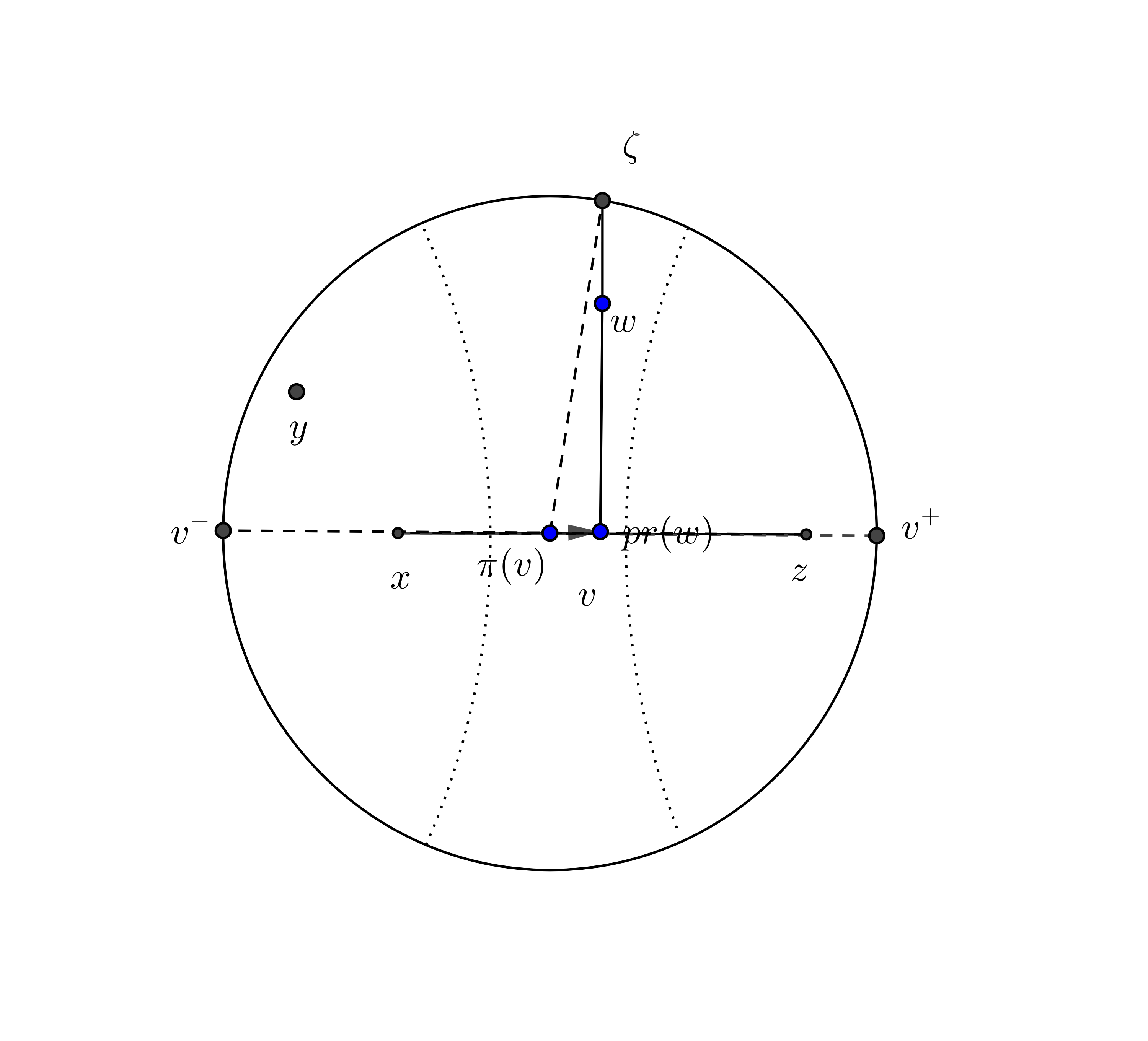
Figure 3. Approximating by Naim kernels

We choose $R=R(x,y,\varepsilon)$ larger than 1 such that the angle between the vectors $v_{pr(w)}^{x}$ and $v_{pr(w)}^{y}$ is small enough if $d(x,pr(w))\geq R$ and that Proposition 3.8 holds for the triples $(x,\pi(v),w),(y,\pi(v),w)$ and $(z,\pi(v),w):$ for $w\notin N_{R}(x)\cup N_{R}(z)$ and $pr(w)$ is far from $w$, independently on $d(x,z)$,

$$\frac{G_{\lambda}(w,z)G_{\lambda}(w,y)}{G_{\lambda}(z,y)G_{\lambda}^{2}(\pi(v),w)}=\frac{\theta^{\lambda}_{\pi(v)}(w,z)\theta^{\lambda}_{\pi(v)}(w,y)}{\theta^{\lambda}_{\pi(v)}(y,z)}\sim^{1+\varepsilon}\frac{\theta^{\lambda}_{\pi(v)}(\zeta,v^{+})\theta^{\lambda}_{\pi(v)}(\zeta,v^{-})}{\theta^{\lambda}_{\pi(v)}(v^{-},v^{+})},$$

where $\zeta$ is the end point of the geodesic going from $pr(w)$ to $w$ (see Figure 3).

Extend the projection $pr$ to the boundary $\partial\widetilde{M}$. Then for $w\notin N_{1}(x)\cup N_{1}(z)$, $\psi(v,w)=\psi(v,\zeta)$. Also, the functions $d_{\pi(v)}(\zeta,v^{\pm})$ are bounded away from 0 and the function $\theta^{\lambda}_{\pi(v)}(\zeta,v^{+})\theta^{\lambda}_{\pi(v)}(\zeta,v^{-})$ is uniformly Hölder and bounded away from 0. The denominator $\theta_{\lambda_{0}}(v)$ is also Hölder and the approximation is uniformly Hölder continuous. Therefore, the map

$$\zeta\mapsto\psi(v,\zeta)\frac{\theta^{\lambda}_{\pi(v)}(\zeta,v^{+})\theta^{\lambda}_{\pi(v)}(\zeta,v^{-})}{\theta^{\lambda}_{\pi(v)}(v^{-},v^{+})}$$

is Hölder continuous uniformly on $v$. By Proposition 5.5 centered at $\pi(v)$, there is $R(\varepsilon)$ and $\delta(\varepsilon)$ such that for $r\geq R(\varepsilon),\lambda\in[\lambda_{0}-\delta(\varepsilon),\lambda_{0}],$ we have $u_{\lambda,r}(v)\;\sim^{1+\varepsilon}\Omega u(v)$, where

(6.4) $$u(v)\;=\;\int_{\partial\widetilde{M}}\psi(v,\zeta)\frac{\theta_{\pi(v)}(\zeta,v^{+})\theta_{\pi(v)}(\zeta,v^{-})}{\theta(v)}d\mu^{\lambda_{0}}_{\pi(v)}(\zeta).$$

In the above equation, $v$ is a vector in the geodesic from $x$ to $z$. Now consider $u$ above as a function on $S\widetilde{M}$ and observe that the right hand side of (6.4) is well-defined $\Gamma$-invariant and positive on $S\widetilde{M}$. Let us denote the induced function on $SM$ by $u$ again.

We claim that the function $u$ is Hölder continuous on $SM$. Indeed, consider two vectors $v_{1},v_{2}\in S\widetilde{M}$ at a small distance $d(v_{1},v_{2})$. For each $t\in[-1,1],$ we associate to $v^{\prime}_{1}=\mathbf{g}_{t}v_{1}$ the vector $v^{\prime}_{2}=\mathbf{g}_{t}v_{2}$. We have $d(v^{\prime}_{1},v^{\prime}_{2})\leq Cd(v_{1},v_{2}).$ We can now pair each vector in $S_{p(v^{\prime}_{1})}\widetilde{M}$ orthogonal to $v^{\prime}_{1}$ with a vector in $S_{p(v^{\prime}_{2})}\widetilde{M}$ orthogonal to $v^{\prime}_{2}$, also within a distance at most $Cd(v_{1},v_{2}).$ By considering their points at infinity, we have paired each $\zeta_{1}\in\partial\widetilde{M}$ such that $\psi(v_{1},\zeta_{1})>0$ with a point $\zeta_{2}\in\partial\widetilde{M}$ such that $\psi(v_{1},\zeta_{1})=\psi(v_{2},\zeta_{2})$ and $d_{p(v_{1})}(\zeta_{1},\zeta_{2})\leq C(d(v_{1},v_{2}))^{\alpha}.$ So, in formula (6.4), the integrand and the measure, which are Hölder continuous in $\zeta$ and smooth in $\pi(v)$ depend Hölder continuously on $v$.

It follows that for $\lambda$ close to $\lambda_{0}$, the function $\overline{u}_{\lambda}$ which is a function of $x,y,z$ satisfies

$$-P(\lambda)\overline{u}_{\lambda}(v)\sim^{1+\varepsilon}-P(\lambda)\Omega u(v)\int_{0}^{\infty}e^{P(\lambda)r}dr=\Omega u(v)$$

independently on $d(x,z)$ and uniformly on $x$ and $y$ as long as $d(x,y)$ is bounded. ∎

Proof of Proposition 6.2.

By (6.3) and Lemma 6.4, it remains to show that the limit

$$\lim_{R\to\infty,\lambda\to\lambda_{0}}\int_{S(x,R)}e^{-P(\lambda)R}G_{\lambda}^{2}(x,z)k_{\lambda}(x,y,z)\left(\frac{1}{R}\int_{0}^{R}u(\mathbf{g}_{s}v_{x}^{z})ds\right)dz,$$

exists uniformly in $\lambda$ where the function $u$ is given by (6.4). As in the proof of Proposition 5.3, we can replace $k_{\lambda}(x,y,z)$ by $k_{\lambda_{0}}(x,y,\sigma_{x}(v_{x}^{z}))$ for $R$ sufficiently large and $\lambda$ close to $\lambda_{0}$. By Proposition 4.12, for $R$ large and $\lambda_{0}-\lambda$ small,

$$e^{-P(\lambda)R}\int_{S(x,R)}G_{\lambda}^{2}(x,z)k_{\lambda_{0}}(x,y,\sigma_{x}(v_{x}^{z}))\left(\frac{1}{R}\int_{0}^{R}u(\mathbf{g}_{s}v_{x}^{z})ds\right)dz\sim\Omega^{2}c(x,y)\int_{SM}u\,dm_{\lambda_{0}}$$

by (5.3). Proposition 6.2 follows since

$$\int_{SM}udm_{\lambda_{0}}=\quad\int_{SM_{0}}\int_{\partial\widetilde{M}}\psi(v,\zeta)\frac{\theta_{\pi(v)}(\zeta,v^{+})\theta_{\pi(v)}(\zeta,v^{-})}{\theta(v)}d\mu^{\lambda_{0}}_{\pi(v)}(\zeta)dm_{\lambda_{0}}(v)$$

$$= \;\int_{SM_{0}}\int_{\partial\widetilde{M}}\psi(v,\zeta)\frac{\theta_{\pi(v)}(\zeta,v^{+})\theta_{\pi(v)}(\zeta,v^{-})}{\theta(v)}d\mu^{\lambda_{0}}_{\pi(v)}(\zeta)\Omega\theta^{2}(v)d\mu^{\lambda_{0}}_{\pi(v)}(v^{-})d\mu^{\lambda_{0}}_{\pi(v)}(v^{+})dt$$

$$= \frac{\Omega}{\Upsilon}\;\int_{\partial\widetilde{M}}\int_{(v^{-},v^{+},t)\in SM_{0}}\psi(v,\zeta)dtd\widetilde{\tau}^{\lambda_{0}}_{\pi(v)}(v^{+},v^{-},\zeta)$$

$$= \frac{\Omega}{\Upsilon}\;\widetilde{\tau}^{\lambda_{0}}_{\pi(v)}(S^{2}M_{0})=\frac{\Omega}{\Upsilon}.$$

Recall that $\widetilde{\tau}^{\lambda_{0}}_{x},\Upsilon$ are defined in (2.12) and (2.13). ∎

Proof of Theorem 6.1.

Set $F(\lambda)=\frac{\partial}{\partial\lambda}G_{\lambda}(x,y)$. By Proposition 5.3 and Proposition 6.2,

$$\lim_{\lambda\to\lambda_{0}}-P(\lambda)F(\lambda)=\Omega\;c(x,y)\;\ \textrm{and}\;\lim_{\lambda\to\lambda_{0}}-P^{3}(\lambda)F^{\prime}(\lambda)=2\frac{\Omega^{3}}{\Upsilon}c(x,y).$$

It follows that $\displaystyle\frac{2F^{\prime}(\lambda)}{F(\lambda)^{3}}$ converges towards $\displaystyle\frac{4}{\Upsilon}(c(x,y))^{-2}.$ Since $F(\lambda)$ goes to $\infty$ as $\lambda\to\lambda_{0}$, we conclude that $F(\lambda)\sim\frac{\sqrt{\Upsilon}}{2}\frac{c(x,y)}{\sqrt{\lambda_{0}-\lambda}}.$ ∎

By Proposition 5.3 and Theorem 6.1, we obtain

Corollary 6.5.

As $\lambda\to\lambda_{0}$,

$$-\frac{P(\lambda)}{\sqrt{\lambda_{0}-\lambda}}\to\frac{2\Omega}{\sqrt{\Upsilon}}.$$

Applying Proposition 6.2 and Corollary 6.5, we get

Corollary 6.6.

For all $x,y\in\widetilde{M},$

$$\lim_{\lambda\to\lambda_{0}}(\lambda_{0}-\lambda)^{3/2}\int_{\widetilde{M}\times\widetilde{M}}G_{\lambda}(x,z)G_{\lambda}(z,w)G_{\lambda}(w,y)d\mathrm{Vol}(z)d\mathrm{Vol}(w)\;=\;\frac{\sqrt{\Upsilon}}{8}c(x,y).$$

Moreover, for any compact neighborhood $K$ of $x$ in $\widetilde{M}$, there is $\lambda^{\prime}<\lambda_{0}$ such that

$$y\mapsto\sup_{\lambda,\lambda^{\prime}\leq\lambda\leq\lambda_{0}}(\lambda_{0}-\lambda)^{3/2}\int_{\widetilde{M}\times\widetilde{M}}G_{\lambda}(x,z)G_{\lambda}(z,w)G_{\lambda}(w,y)d\mathrm{Vol}(z)d\mathrm{Vol}(w)$$

is integrable on $K$.

6.2. Proof of Theorem 1.1 and Theorem 1.7

The proof relies on the following Proposition, based on Hardy-Littlewood Tauberian Theorem:

Proposition 6.7.

Fix $x_{0}\in\widetilde{M}$. Let $F$ be a nonnegative $C^{\infty}$ function on $\widetilde{M}$, with compact support. Then,

$$\lim\limits_{t\to\infty}t^{3/2}\int_{\widetilde{M}\times\widetilde{M}}e^{\lambda_{0}t}\wp(t,x,y)F(x)F(y)\,d\mbox{Vol}(x)d\mbox{Vol}(y)$$

$$\quad=\;\frac{\sqrt{\Upsilon}}{4}\int_{\widetilde{M}\times\widetilde{M}}c(x,y)F(x)F(y)\,d\mbox{Vol}(x)d\mbox{Vol}(y),$$

where $c(x,y)$ is given by (5.3).

Proof.

Set $\mu_{F}$ for the spectral measure of $F$, i.e. the Borel finite measure on the spectrum $[0,+\infty)$ of $\Delta-\lambda_{0}$ such that, for all $m\geq 0$,

$$\int_{{\widetilde{M}}}F(x)\Delta^{m}F(x)\,d\mbox{Vol}(x)\;=\;\int_{0}^{+\infty}(\varpi-\lambda_{0})^{m}\,d\mu_{F}(\varpi).$$

The function

$$c_{F}(t)\;:=\;\int_{\widetilde{M}\times\widetilde{M}}e^{\lambda_{0}t}\wp(t,x,y)F(x)F(y)\,d\mbox{Vol}(x)d\mbox{Vol}(y)=\int_{0}^{+\infty}e^{-\varpi t}\,d\mu_{F}(\varpi)$$

is nonincreasing in $t$. It satisfies the following property

Lemma 6.8.

For all $s>0$,

$$\int_{0}^{+\infty}e^{-st}t^{2}c_{F}(t)\,dt=2\int_{\widetilde{M}^{4}}G_{\lambda_{0}-s}(x,z)G_{\lambda_{0}-s}(z,w)G_{\lambda_{0}-s}(w,y)F(x)F(y)\,d{\mathrm{Vol}}^{4}(z,w,x,y).$$

Proof.

On the one hand, we have

$$\int_{0}^{+\infty}e^{-st}t^{2}c_{F}(t)\,dt\;=\;\int_{\widetilde{M}\times\widetilde{M}}\int_{0}^{\infty}t^{2}e^{(\lambda_{0}-s)t}\wp(t,x,y)dtF(x)F(y)\,d\mbox{Vol}(x)d\mbox{Vol}(y).$$

On the other hand, we may write

$$2\int_{\widetilde{M}^{4}}G_{\lambda_{0}-s}(x,z)G_{\lambda_{0}-s}(z,w)G_{\lambda_{0}-s}(w,y)F(x)F(y)\,d{\mathrm{Vol}}^{4}(z,w,x,y)$$

$$= 2\int_{\widetilde{M}^{4}\times\mathbb{R}_{+}^{3}}e^{(\lambda_{0}-s)(t+u+v)}\wp(t,x,z)\wp(u,z,w)\wp(v,w,y)\,dtdudvF(x)F(y)\,d{\mathrm{Vol}}^{4}(z,w,x,y)$$

Introducing the variables $u+v=:r$ and $t+r=:\tau$ and using the semigroup property of the heat kernel, we obtain

$$\int_{\widetilde{M}^{2}}\left(\int_{0}^{\infty}\tau^{2}e^{(\lambda_{0}-s)\tau}\wp(\tau,x,y)\,d\tau\right)F(x)F(y)\,d\mbox{Vol}^{2}(x,y).$$

∎

By Corollary 6.6 and Lemma 6.8 we have, as $s\to 0,$

$$s^{3/2}\int_{0}^{+\infty}e^{-st}t^{2}c_{F}(t)\,dt\to\frac{\sqrt{\Upsilon}}{4}\int_{\widetilde{M}\times\widetilde{M}}c(x,y)F(x)F(y)\,d\mbox{Vol}(x)d\mbox{Vol}(y).$$

By Hardy-Littlewood Tauberian Theorem ([F] p. 445), as $T\to\infty$, we have

(6.5) $$\int_{0}^{T}t^{2}c_{F}(t)dt\;\sim\;\frac{\sqrt{\Upsilon}}{4\Gamma(5/2)}T^{3/2}\int_{\widetilde{M}\times\widetilde{M}}c(x,y)F(x)F(y)\,d\mbox{Vol}(x)d\mbox{Vol}(y).$$

Now we claim that

$$c_{F}(t)\sim\frac{\sqrt{\Upsilon}}{2\sqrt{\pi}t^{3/2}}\int_{\widetilde{M}\times\widetilde{M}}c(x,y)F(x)F(y)\,d\mbox{Vol}(x)d\mbox{Vol}(y).$$

Indeed, by setting $\Xi T^{3/2}$ to be the right hand side of the equation (6.5), we have, for all $\varepsilon>0$,

$$\int_{T}^{T(1+\varepsilon)}t^{2}c_{F}(t)dt\;=\;T^{3/2}\Xi(1+\varepsilon)^{3/2}-\Xi T^{3/2}+o(T^{3/2})=\Xi T^{3/2}((1+\varepsilon)^{3/2}-1+o(1)).$$

On the other hand, since $c_{F}(t)$ is a non-increasing function of $t$, for $\varepsilon>0$ small,

$$\int_{T}^{T(1+\varepsilon)}t^{2}c_{F}(t)dt\leq c_{F}(T)\int_{T}^{T(1+\varepsilon)}t^{2}dt=c_{F}(T)T^{3}(\varepsilon+\varepsilon^{2}+\varepsilon^{3}/3).$$

Comparing the two inequalities yields:

$$\liminf_{T\to\infty}c_{F}(T)T^{3/2}\;\geq\;\frac{3\Xi}{2}+o(\varepsilon).$$

One shows in the same way, using $\int_{T(1-\varepsilon)}^{T}$, that $\limsup_{T\to\infty}c_{F}(T)T^{3/2}\;\leq\;\frac{3\Xi}{2}.$ This proves Proposition 6.7. ∎

Proof of Theorem 1.1 and Theorem 1.7..

Since $c(x,y)=\int k_{\lambda_{0}}(x,y)d\mu_{x}$, and $k_{\lambda_{0}}(x,y)$ is smooth as a $\lambda_{0}$-harmonic function, the function $c(x,y)$ is smooth in $x$ and $y$. Moreover, by Proposition 8.4 below, $\log\wp(t,x,y)$ has bounded gradient, uniformly in $t$ large. We can therefore apply Proposition 6.7 to functions $F$ with compact support such that the measures $F(x)d\mathrm{Vol}(x)$ converge to the Dirac measure $\delta_{x_{0}}$ to get

$$\lim\limits_{t\to\infty}t^{3/2}e^{\lambda_{0}t}\wp(t,x_{0},x_{0})\;=\;\frac{\sqrt{\Upsilon}}{2\sqrt{\pi}}c(x_{0},x_{0}).$$

We get the general case of $x_{0}\not=x_{1}$ of Theorem 1.1 and Theorem 1.7 in the same way by applying Proposition 6.7 to functions that approximate $\delta_{x_{0}}+\delta_{x_{1}}.$ ∎

7. Appendix I: Uniform mixing

In this section, we establish a uniform power mixing of the geodesic flow for Gibbs measures, when the potential varies in a neighbourhood of the space $\mathcal{K}_{\alpha}$ of functions which will be defined shortly. The proof combines the ideas from [P1] and [P2], with a slightly different framework. For the comfort of the reader, we recall the different steps in our notations.

7.1. Uniform mixing and three-mixing

Let $\mathbb{X}:=(X,\mathcal{A},m;{\mathbf{g}}_{t},t\in\mathbb{R})$ be a system with a one parameter group $\{{\mathbf{g}}_{t},t\in\mathbb{R}\}$ of measurable transformations of the space $(X,\mathcal{A})$ preserving a probability measure $m$. For bounded measurable functions $f,g,h$ we define the correlations functions for $s,t\geq 0$:

$$\rho_{f,g,m}(t) = \int f(x)g({\mathbf{g}}_{t}x)dm(x)-\int f\,dm\int g\,dm$$

$$\rho_{f,g,h,m}(s,t) = \int f(x)g({\mathbf{g}}_{s}x)h({\mathbf{g}}_{s+t}x)dm(x)-\int f\,dm\int g\,dm\int h\,dm$$

$$\overline{\rho}_{f,g,h,m}(t) = \frac{1}{t}\int_{0}^{t}\left[\int f(x)g({\mathbf{g}}_{s}x)h({\mathbf{g}}_{t}x)dm(x)\right]ds-\int f\,dm\int g\,dm\int h\,dm$$

The system $\mathbb{X}$ is called mixing if $\lim_{t\to\infty}\rho_{f,g,m}(t)=0$ for all bounded functions $f,g$, 3-mixing if $\lim_{s,t\to\infty}\rho_{f,g,h,m}(s,t)=0$ for all bounded functions $f,g,h$ and average 3-mixing if $\lim_{t\to\infty}\overline{\rho}_{f,g,h,m}(t)=0$ for all bounded functions $f,g,h$. It is a well-known open problem whether mixing implies 3-mixing. It is easy to see that mixing implies average 3-mixing.

Let us consider the rate of mixing. A system $\mathbb{X}$ is called power mixing for a class $\mathcal{K}$ of functions if for $f,g\in\mathcal{K}$, $\rho_{f,g,m}(t)$ decays polynomially (see Theorem 7.2 for a precise statement). Below, we will show a uniform version of a power mixing of the geodesic flow for the class $\mathcal{K}=\mathcal{K}_{\alpha}$ which we define now.

Let $\alpha>0$. We denote $\mathcal{K}_{\alpha}$ the space of functions $f$ on $X$ such that $\|f\|_{\alpha}<\infty$, where

$$\|f\|_{\alpha}:=\sup_{x}|f(x)|+\sup_{x\not=y}\frac{|f(x)-f(y)|}{(d(x,y))^{\alpha}}.$$

From now on, let ${\mathbf{g}}_{t}$ be an Anosov flow. For any potential function $\varphi\in\mathcal{K}_{\alpha}$, there is a unique invariant probability measure $m_{\varphi}$ attaining the supremum of the mesure theoretic pressure $h_{m}({\mathbf{g}})+\int\varphi dm$ in the set $\Omega$ of all ${\mathbf{g}}_{t}$-invariant Borel probability measures, i.e.:

$$P(\varphi):=\sup_{m\in\Omega}\left\{h_{m}({\mathbf{g}})+\int\varphi\,dm\right\}=h_{m_{\varphi}}({\mathbf{g}})+\int\varphi\,dm_{\varphi},$$

where $h_{m}({\mathbf{g}})$ denotes the measure theoretic entropy of $m$ (see e.g. [PP]). The quantity $P(\varphi)$ is called the topological pressure of the potential function $\varphi$. The mapping $\varphi\mapsto m_{\varphi}$ is continuous from $\mathcal{K}_{\alpha}$ to the space of measures on $X$ endowed with the weak* topology.

The following property is important in Dolgopyat’s approach to the speed of mixing.

Definition 7.1.

A system $\mathbb{X}$ is topologically power mixing if there exists $t_{0},\delta>0$ such that for any $r$, and $t>\max\{\frac{1}{r^{\delta}},t_{0}\}$, and any $x,y$,

$${\mathbf{g}}_{t}(B(x,r))\cap B(y,r)\neq\emptyset.$$

We now establish a local uniform power mixing for topologically power mixing Anosov flows, for Gibbs measures associated to potentials $\varphi$, and for functions in $\mathcal{K}_{\alpha}$. The mixing rate is uniform as we vary the potential $\varphi$ in a small neighbourhood in $\mathcal{K}_{\alpha_{0}}$, for $\alpha$ and $\alpha_{0}$ sufficiently small.

Theorem 7.2.

Let $\mathbb{X}$ be a topologically power mixing Anosov flow. There exists $\alpha_{0}>0$ with the following property: let $\varphi_{0}\in\mathcal{K}_{\alpha_{0}}(X)$ be a potential. There exist $\varepsilon>0$, $\alpha>0$ and $C^{\prime}_{0},c^{\prime}_{0}>0$ such that for all $\varphi$ with $||\varphi-\varphi_{0}||_{\alpha_{0}}<\varepsilon$ and all $f,g,h\in\mathcal{K}_{\alpha},$ we have, for all positive $s,t$:

(7.1) $$\big{|}\rho_{f,g,h,m_{\varphi}}(s,t)\big{|}\;\leq\;C^{\prime}_{0}\|f\|_{\alpha}\|g\|_{\alpha}\|h\|_{\alpha}[(1+s)^{-c^{\prime}_{0}}+(1+t)^{-c^{\prime}_{0}}].$$

Proposition 7.3.

Let $\mathbb{X}$ be a topologically power mixing Anosov flow. There exists $\alpha_{0}>0$ with the following property: let $\varphi_{0}\in\mathcal{K}_{\alpha_{0}}(X)$ be a potential. There exist $\varepsilon>0$, $\alpha>0$ and $C,c>0$ such that for all $\varphi$ with $||\varphi-\varphi_{0}||_{\alpha_{0}}<\varepsilon$ and all $f,g\in\mathcal{K}_{\alpha},$ we have, for all positive $t$:

(7.2) $$\big{|}\rho_{f,g,m_{\varphi}}(t)\big{|}\;\leq\;C\|f\|_{\alpha}\|g\|_{\alpha}(1+t)^{-c}.$$

Corollary 7.4.

Let $\mathbb{X}$ be a topologically power mixing Anosov flow. There exists $\alpha_{0}>0$ with the following property: let $\varphi_{0}\in\mathcal{K}_{\alpha_{0}}(X)$ be a potential. There exist $\varepsilon>0$, $\alpha>0$ and $C^{\prime}_{0},c^{\prime}_{0}>0$ such that for all $\varphi$ with $||\varphi-\varphi_{0}||_{\alpha_{0}}<\varepsilon$ and all $f,g,h\in\mathcal{K}_{\alpha},$ we have, for all positive $t$:

(7.3) $$\big{|}\overline{\rho}_{f,g,h,m_{\varphi}}(t)\big{|}\;\leq\;C_{0}^{\prime}\|f\|_{\alpha}\|g\|_{\alpha}\|h\|_{\alpha}(1+t)^{-c_{0}^{\prime}}.$$

We assume now that the system $\mathbb{X}$ is the geodesic flow $\mathbf{g}_{t},t\in\mathbb{R}$ on the unit tangent bundle $X=SM$, where $M$ is a closed negatively curved manifold.

Liverani proved exponential mixing for contact Anosov flows for the Liouville measure, which implies exponential mixing for the geodesic flow on manifolds of negative curvature for the Liouville measure [Li]. It implies that the geodesic flow is topologically power mixing. Thus we can apply the above theorems to the geodesic flow and the Gibbs measure associated to $\varphi_{\lambda_{0}}$ to obtain Propositions 4.1 and 4.2.

7.2. Proof of Theorem 7.2 and Proposition 10

First, following Bowen and Ruelle [B], [BR], we can reduce the problem to the corresponding problem on suspended symbolic flows by introducing Poincaré sections for the flow with Markov property (see also [PP] Chapter 9 and Appendix III), in such a way that Hölder continuous functions on $SM$ correspond to Hölder continuous functions on the symbolic system. (The Hölder constant might change, say from $\alpha_{0}$ to $2\alpha$.)

We may thus assume that there is a subshift of finite type $(\Sigma,\sigma)$ and a positive $\alpha$-Hölder continuous function $\tau$ on $\Sigma$ such that the system $\mathbb{X}$ is the suspension flow $\sigma_{t}(x,r)=(x,r+t)$ on the set $\Sigma^{\tau}:=\{(x,r):x\in\Sigma,0\leq r\leq\tau(x)\}/[(x,\tau(x))\sim(\sigma x,0)].$ Let us denote by $[a_{0},\cdots,a_{k}]$ the cylinder set $\{x:x_{i}=a_{i},i=0,\cdots,k\}$. Let us also define $d_{\alpha}$ on the space $\Sigma_{+}$ of one-sided sequences with the left-shift by $d_{\alpha}(x,y)=\alpha^{k}$, where $k$ is the first index for which $x_{k},y_{k}$ are not equal. Let us denote by $\mathcal{K}_{\alpha}(\Sigma_{+})$ the space of $d_{\alpha}$-Lipschitz functions on the space $\Sigma_{+}$ of one-sided sequences. Let $\varphi\in\mathcal{K}_{2\alpha}(\Sigma^{\tau})$ be a potential function on $\Sigma^{\tau}$. Then the function $\int_{0}^{\tau(x)}\varphi(x,r)\,dr$ is $d_{2\alpha}$-Lipschitz on $\Sigma.$

We may assume that the function $\tau$ is a function on $\Sigma_{+}$ in the sense that $\tau(x)=\tau(y)$ if the points $x$ and $y$ in $\Sigma$ have the same nonnegative coordinates. Moreover, the function $\tau$ is a $d_{\alpha}$-Lipschitz function on $\Sigma_{+}$. The function $\phi_{1}$ on $\Sigma_{+}$ associated to $\int_{0}^{\tau(x)}\varphi(x,r)\,dr$ is a $d_{\alpha}$-Lipschitz function ([Sin], [Bo], see also Proposition 1.2 of [PP] for example). Now normalize $\phi_{1}$ to obtain a $d_{\alpha}$-Lipschitz function $\phi$ with ${\mathcal{L}}_{\phi}1=1$, where

(7.4) $${\mathcal{L}}_{\phi}F(x):=\sum_{y;\sigma y=x}e^{\phi(y)}F(y)$$

is the transfer operator associated to $\phi$ (see e.g. [PP] page 115 for these classical reductions). We conclude that the map $\mathcal{T}$ sending $\varphi$ to $\phi$ is continuous from $\mathcal{K}_{\alpha_{0}}(SM)$ into $\mathcal{K}_{\alpha}(\Sigma_{+})$. The equilibrium measure $m_{\varphi}$ for the function $\varphi$ is of the form

$$m_{\varphi}=\frac{1}{\int\tau\,d\nu_{\phi}}(\overline{\nu}_{\phi}\otimes dr)\big{|}_{\Sigma^{\tau}},$$

where $\overline{\nu}_{\phi}$ is the unique $\sigma$-invariant probability measure on $\Sigma$ such that its projection $\nu_{\phi}$ to $\Sigma_{+}$ satisfies, for all functions $F\in C(\Sigma_{+})$,

(7.5) $$\int{\mathcal{L}}_{\phi}F\,d\nu_{\phi}=\int F\,d\nu_{\phi}.$$

Let us denote $\phi^{(k)}(x)=\phi(x)+\phi(\sigma(x))+\cdots+\phi(\sigma^{k-1}(x))$. For a given $\varphi_{0}$, we choose an $\varepsilon_{1}$-neighborhood of $\phi_{0}=\mathcal{T}\varphi_{0}$ so that there exists a constant $C_{1}\geq 1$ with, for all normalized $\phi$ in the $\varepsilon_{1}$-neighborhood of $\phi_{0},$ all $k\in{\mathbb{N}},$

(7.6) $$\left|\frac{e^{\phi^{(k)}(x)}}{e^{\phi^{(k)}(y)}}-1\right|\leq C_{1}\alpha^{-k}d_{\alpha}(x,y),\quad\forall x,y\in\Sigma_{+}$$

(7.7) $$\mathrm{and}\;\;C_{1}^{-1}\leq\frac{\nu_{\phi}[a_{0},\cdots,a_{k-1}]}{e^{\phi^{(k)}(x)}}\leq C_{1},\quad\forall x\in[a_{0},\cdots,a_{k-1}].$$

With those choices, for all $\phi$, 1 is an isolated eigenvalue of ${\mathcal{L}}_{\phi}$ with eigenfunction the constant 1 (see [PP], Theorem 2.2 page 21). A ball of radius $r$ in $\Sigma^{\tau}$ contains a cylinder of length $-C\log r$ in $\Sigma$ times an interval of length $cr$ in the flow direction. Its image on the manifold contains a ball of radius $r^{D}$, for some $D$. Therefore, the suspension flow $\mathbb{X}$ is topologicallly power mixing for the symbolic distance.

Remark 7.5.

The rest of the proof in this section follows the ideas of D. Dolgopyat ([D2]). In order to check that all the arguments are uniform for equilibrium measures $m_{\varphi}$ for $\varphi$ in a neighborhood of $\varphi_{0}$, we found it more convenient to follow [Me]. In particular, the constants $C_{1},C_{6},C_{7},\gamma_{3}$ in this section coincide with those in [Me].

7.2.1. Properties of the complex transfer operator

In this subsection, we will denote the space of complex $d_{\alpha}$-Lipschitz continuous functions on $\Sigma_{+}$ by $\mathcal{K}_{\alpha}(\Sigma_{+})$ again. Let $\phi\in\mathcal{K}_{\alpha}(\Sigma_{+})$ with ${\mathcal{L}}_{\phi}1=1$. We define the complex transfer operator ${\mathcal{L}}_{\phi+s\tau},s\in\mathbb{C}$ on $\mathcal{K}_{\alpha}(\Sigma_{+})$ by

$${\mathcal{L}}_{\phi+s\tau}F(x):=\sum_{y;\sigma y=x}e^{\phi(y)+s\tau(y)}F(y).$$

Following [Me], set $s=a+ib$.

We recall that, by mixing of the geodesic flow, $\|{\mathcal{L}}_{\phi+ib\tau}\|_{\alpha}<1$ for $b\neq 0$ (see [PP] Proposition 6.2). In particular, for $b\neq 0,$ the series $\sum_{n}{\mathcal{L}}^{n}_{\phi+ib\tau}$ converges as a series of operators in $\mathcal{K}_{\alpha}(\Sigma_{+}).$ The sum $\sum_{n}{\mathcal{L}}^{n}_{\phi+s\tau}=(I-{\mathcal{L}}_{\phi+s\tau})^{-1}$ depends analytically on $s=a+ib$ for $a<0$ and has a continuous extension to $a=0,b\neq 0$. Dolgopyat’s method allows to extend analytically that sum beyond the imaginary axis (Propositions 7.6 and 7.7).

Proposition 7.6.

There is $\delta=\delta_{\phi_{0}}>0,\varepsilon>0$ such that, for all normalized $\phi$ with $||\phi-\phi_{0}||_{\alpha}<\varepsilon$, the mapping $s\mapsto\sum_{n}{\mathcal{L}}^{n}_{\phi+s\tau}$ is meromorphic on $V_{\delta},$ where

$$V_{\delta}:=\{s=a+ib:|b|<2,\;|a|<\delta\}$$

with a simple pole at $s=0$. Moreover, for a function $K\in\mathcal{K}_{\alpha}(\Sigma_{+}),$ the residue at $s=0$ of the meromorphic function $s\mapsto\sum_{n}{\mathcal{L}}^{n}_{\phi+s\tau}K$ (with values in $\mathcal{K}_{\alpha}$) is a constant function with value $\nu_{\phi}(K).$

Proof.

For a fixed $\phi$ , this follows from [PP], Proposition 6.2 and Theorem 10.2, with a fixed $\delta=\delta_{\phi}$. By [Ka] Theorem IV.3.1 and compactness of the closure $\overline{V_{\delta}}$, there is a neighborhood $\mathcal{U}_{0}$ of $\phi_{0}$ such that for normalized $\phi\in\mathcal{U}_{0}$, the rest of the spectrum of ${\mathcal{L}}_{\phi+s\tau},s\in\overline{V_{\delta}},$ is separated from 1 by $\delta=\delta_{\phi_{0}}$. ∎

Proposition 7.7.

(Compare with Lemma 3.5 of [Me]) Let $\mathbb{X}$ be a topologically power mixing Anosov flow. Let $\phi_{0}$ be a $\alpha$-Hölder continuous function. There exist constants $\varepsilon,\delta,\beta,D_{0}$ such that, for all normalized $\phi,\|\phi-\phi_{0}\|_{\alpha}<\varepsilon,$ the series of operators $\sum_{n}{\mathcal{L}}^{n}_{\phi+s\tau}$ has an analytic extension on the region $U=U_{\delta,\beta}$, where

$$U_{\delta,\beta}\;:=\;\{s,s=a+ib;|b|>1,\;|a|<\frac{2\delta}{|b|^{\beta/2}}\}$$

and, for $s\in U,$

(7.8) $$\|\sum_{n}{\mathcal{L}}^{n}_{\phi+s\tau}\|_{\alpha}\;\leq\;D_{0}|b|^{D_{0}}.$$

Proof.

As in [Me], we carry the calculations for $0\leq a\leq 1$ and $b>1$. They are analogous for $b<-1$ and for $-1\leq a\leq 0.$ More precisely, we find a neighborhood $\mathcal{U}$ of $\phi_{0}$ and $\theta>0,C>0$ such that the conclusion holds for all $s=a+ib$ with $|b|>1,$ $|a|<C^{-1}|b|^{-\theta}$, and for all normalized $\phi\in\mathcal{U}$. We first have the preliminary estimate of [Me] in a uniform way.

Lemma 7.8.

(Lemma 3.7 of [Me]) There exist $C_{6},C_{7},\gamma_{3},\varepsilon_{2}>0$ such that for all normalized $\phi$ with $||\phi-\phi_{0}||_{\alpha}<\varepsilon_{2}$,

1. $|{\mathcal{L}}_{\phi+ib\tau}|_{\infty}\leq 1,$

2. $||{\mathcal{L}}_{\phi+ib\tau}^{n}F||_{\alpha}\leq C_{6}\{b|F|_{\infty}+\alpha^{n}||F||_{\alpha}\}$ for all $n\geq 1$ and $F\in\mathcal{K}_{\alpha}(\Sigma_{+})$,

3. $||{\mathcal{L}}_{\phi}^{n}F-\int_{\Sigma_{+}}Fd\nu_{\phi}||_{\alpha}\leq C_{7}\gamma_{3}^{n}||F||_{\alpha}$ for all $n\geq 1$ and $F\in\mathcal{K}_{\alpha}(\Sigma_{+})$.

Proof.

Part (2) comes from the basic inequality ([PP], Proposition 2.1) thus $C_{6}$ is uniform in $\phi$. Part (3) comes from the spectral gap of ${\mathcal{L}}_{\phi}$ thus $C_{7}$ and $\gamma_{3}$ can be chosen uniformly in a neighbourhood of $\phi_{0}$ (see e.g. Kato [Ka] Theorem IV.3.1). ∎

As in [Me], define

$$\|f\|_{b}:=\max\left\{|f|_{\infty},\frac{1}{2C_{6}b}\sup_{x\not=y}\frac{|f(x)-f(y)|}{(d(x,y))^{\alpha}}\right\}.$$

Since one may assume that $2C_{6}b>1$, we have

$$||F||_{b}\leq||F||_{\alpha}\leq(2C_{6}b+1)||F||_{b},$$

which implies that $||{\mathcal{L}}||_{\alpha}/||{\mathcal{L}}||_{b}$ lies between $2C_{6}b+1$ and $(2C_{6}b+1)^{-1}$.

Let $M_{b}F=e^{-ib\tau}F\circ\sigma$.

Definition 7.9.

The operator $M_{b}$ has no approximate eigenfunction if there exists $N\in{\mathbb{N}}$ such that for every triple $(\theta\geq N,\beta>0,C\geq 1)$, there exists $k=k(\theta,\beta,C)$ such that for all $(b,\rho,F)$ with $|F|=1,\rho\in\mathbb{R}$ and $|b|>k$,

$$|M_{b}^{\beta\log|b|}F(y)-e^{i\rho}F(y)|\geq C|b|^{-\theta},$$

for some $y$.

Lemma 7.10 (Uniform version of Section 3.2 of [Me]).

Consider the following conditions.

1. $M_{b}$ has no approximate eigenfunction.

2. There exist constants $\varepsilon,D$ such that, for all normalized $\phi$ with $||\phi-\phi_{0}||_{\alpha}<\varepsilon$, and $b>1,$ the series of operators $\sum_{n}{\mathcal{L}}^{n}_{\phi+ib\tau}$ satisfies

   $$\|\sum_{n}{\mathcal{L}}^{n}_{\phi+ib\tau}\|_{b}\;\leq\;D|b|^{D}.$$

3. There exist constants $\varepsilon,\delta,\beta,D_{0}$ such that, for all normalized $\phi$ with $||\phi-\phi_{0}||_{\alpha}<\varepsilon$, the function $s\mapsto\sum_{n}{\mathcal{L}}^{n}_{\phi+s\tau}$ has an analytic extension to the region $U_{\delta,\beta}$ and for $s\in U_{\delta,\beta},$

   $$\|\sum_{n}{\mathcal{L}}^{n}_{\phi+s\tau}\|_{b}\;\leq\;D_{0}|b|^{D_{0}}.$$

With the above notations, (1) implies (2) and (2) implies (3).

Proof.

See Section 3.2 of [Me]. Let $\varepsilon_{1}$ be a constant such that $C_{1}$ in equation  (7.6) and $\alpha_{1},\alpha_{2}$ in [Me] are uniform in $\phi$ in $\varepsilon_{1}$-neighborhood of $\phi_{0}$. Now let $\varepsilon=\min\{\varepsilon_{1},\varepsilon_{2}\}$, where $\varepsilon_{2}$ is chosen as in Lemma 7.8. ∎

We now achieve the proof of Proposition 7.7: topologically power mixing of $\mathbb{X}$ implies that $M_{b}$ has no approximate eigenfunction by Sections 3 and 5 of [D2], thus Proposition 7.7 follows. ∎

7.2.2. One-sided smooth functions

We start by proving Theorem 7.2 for a particular space of functions. For $\alpha>0$ and $M\in{\mathbb{N}}$, let $\mathcal{K}_{\alpha,M}^{+}$ be the set of functions $f$ on $\Sigma^{\tau}$ with the following properties:

• for all $x\in\Sigma,$ $f(x,r)=0$ for $r$ outside the interval $[\frac{\inf\tau}{3},\frac{2\inf\tau}{3}]$,

• for all $x\in\Sigma,$ $r\mapsto f(x,r)$ is of class $C^{M}$,

• for all $r\in[\frac{\inf\tau}{3},\frac{2\inf\tau}{3}]$, $x\mapsto f(x,r)$ depends only on the nonnegative coordinates of $x$ and

• the functions $\frac{\partial^{k}f}{\partial r^{k}}(x,r)$, for $0\leq k\leq M$ are $\alpha$-Hölder continuous in $x\in\Sigma$ and continuous in $r$.

For $f\in\mathcal{K}_{\alpha,M}^{+}$, we denote $||f||_{\alpha,M}\textlnot\textdagger:=\sup_{r,k\leq M}||\frac{\partial^{k}f}{\partial r^{k}}(.,r)||_{\alpha}.$ The heart of the proof uses the arguments of [D2] to establish:

Proposition 7.11.

Let $\phi_{0}\in\mathcal{K}_{\alpha}(\Sigma_{+})$as above. There exist $\varepsilon,C,c>0$ and $M$ such that for all $\phi,\|\phi-\phi_{0}\|_{\alpha}<\varepsilon$, all $f,g,h\in\mathcal{K}_{\alpha,M}^{+},$ we have, for all positive $t_{1},t_{2}$:

(7.9) $$\big{|}\rho_{f,g,h,m_{\varphi}}(t_{1},t_{2})\big{|}\;\leq\;C\|f\|_{\alpha,M}\|g\|_{\alpha,M}\|h\|_{\alpha,M}[(1+t_{1})^{-c}+(1+t_{2})^{-c}].$$

Proof.

Choose $\varepsilon$ so that Proposition 7.7 and Proposition 7.6 holds for all $\phi$ with $\|\phi-\phi_{0}\|<\varepsilon$. Fix $f,g,h,\phi$ and write $\rho(t_{1},t_{2})$ for $\rho_{f,g,h,m_{\varphi}}(t_{1},t_{2}).$ Assume first that $\int f\,dm_{\varphi}=\int h\,dm_{\varphi}=0.$ We consider the Laplace transform

$$\widehat{\rho}(s_{1},s_{2})=\int_{\mathbb{R}_{+}\times\mathbb{R}_{+}}\rho(t_{1},t_{2})e^{-s_{1}t_{1}}e^{-s_{2}t_{2}}\,dt_{1}\,dt_{2}$$

which makes sense a priori for $a_{j}>0,$ where $s_{j}=a_{j}+ib_{j},j=1,2.$ The following computation is valid for $a_{j}>0$ and will allow us to extend $\widehat{\rho}(s_{1},s_{2})$ analytically to a larger domain and deduce the decay of $\rho(t_{1},t_{2})$ as $t_{1},t_{2}$ go to infinity.

Lemma 7.12.

Consider the Laplace transforms $F,G$ and $H$ of the functions $f,g$ and $h$ given by:

$$F(x,s)=\int_{\mathbb{R}}e^{-sr}f(x,r)dr,\;G(x,s)=\int_{\mathbb{R}}e^{-sr}g(x,r)dr,\;H(x,s)=\int_{\mathbb{R}}e^{-sr}h(x,r)dr.$$

Then, we have, for $a_{1},a_{2}>0$:

$$\widehat{\rho}(s_{1},s_{2})=\sum_{n,m}\int_{\Sigma}H(x,s_{2}){\mathcal{L}}^{m}_{\phi-s_{2}\tau}\big{[}G(.,s_{1}-s_{2}){\mathcal{L}}^{n}_{\phi-s_{1}\tau}F(.,-s_{1})(.)\big{]}(x)\,d\nu_{\phi}(x).$$

Proof.

We develop:

$$\widehat{\rho}(s_{1},s_{2}) = \int_{\mathbb{R}_{+}\times\mathbb{R}_{+}}\int_{\Sigma^{\tau}}f(x,r)g(\sigma_{t_{1}}(x,r))h(\sigma_{t_{1}+t_{2}}(x,r))e^{-s_{1}t_{1}}e^{-s_{2}t_{2}}\,dm_{\varphi}(x,r)\,dt_{1}\,dt_{2}$$

$$= \sum_{n,m}\int_{\mathbb{R}_{+}\times\mathbb{R}_{+}\times\mathbb{R}_{+}}\int_{\Sigma}f(x,r)g(\sigma^{n}x,r+t_{1}-\tau^{n}(x))h(\sigma^{n+m}x,r+t_{2}+t_{1}-\tau^{n+m}(x))$$

$$\quad\quad\quad\quad\quad\quad\quad\quad\quad\quad\quad\quad\quad\quad\quad\quad e^{-s_{1}t_{1}}e^{-s_{2}t_{2}}\,dr\,d\nu_{\phi}(x)\,dt_{1}\,dt_{2},\quad\quad\quad(*)$$

where $\tau^{n}(x):=\sum_{k=0}^{n-1}\tau(\sigma^{k}(x))$. Observe that for all fixed positive $n,m$ the integral in $t_{1},t_{2},r$ is also an integral over $\mathbb{R}\times\mathbb{R}\times\mathbb{R}.$ Then using the variables $w=r+t_{1}-\tau^{n}(x)$ and $z=w+t_{2}-\tau^{m}(\sigma^{n}x)$, the integral (*) can be written as

$$(*)=\int_{\Sigma}H(\sigma^{n+m}x,s_{2})e^{-s_{2}\tau^{m}(\sigma^{n}x)}G(\sigma^{n}x,s_{1}-s_{2})e^{-s_{1}\tau^{n}(x)}F(x,-s_{1})\,d\nu_{\phi}(x).$$

Using now the invariance of $\nu_{\phi}$ under ${\mathcal{L}}_{\phi}$ (7.5) and the fact that ${\mathcal{L}}^{n}(HK\circ\sigma^{n})(x)=K(x){\mathcal{L}}(H)(x),$ we obtain:

$$(*) = \int_{\Sigma}H(\sigma^{m}x,s_{2})e^{-s_{2}\tau^{m}(x)}G(x,s_{1}-s_{2}){\mathcal{L}}^{n}_{\phi-s_{1}\tau}F(\cdot,-s_{1})(x)\,d\nu_{\phi}(x)$$

$$= \int_{\Sigma}H(x,s_{2}){\mathcal{L}}^{m}_{\phi-s_{2}\tau}\big{[}G(\cdot,s_{1}-s_{2}){\mathcal{L}}^{n}_{\phi-s_{1}\tau}F(\cdot,-s_{1})(\cdot)\big{]}(x)\,d\nu_{\phi}(x).$$

The Lemma follows for $a_{j}=\Re\,s_{j}>0.$ ∎

By Proposition 7.7 and our choice of $\varepsilon$, we conclude that there exist constants $\delta,\beta,D_{0}$ such that, for all normalized $\phi$ with $||\phi-\phi_{0}||_{\alpha}<\varepsilon$, the mapping $s\mapsto\sum_{n}{\mathcal{L}}^{n}_{\phi+s\tau}$ extends analytically on the region $U_{\delta,\beta}$ and, for $s\in U_{\delta,\beta},$

(7.10) $$\|\sum_{n}{\mathcal{L}}^{n}_{\phi+s\tau}\|_{\alpha}\;\leq\;D_{0}|b|^{D_{0}}.$$

Moreover, by Proposition 7.6, there is $\delta>0$ such that the series of operators $\sum_{n}{\mathcal{L}}^{n}_{\phi+s\tau}$ converges and is meromorphic on the region $V_{\delta}$, has a simple pole at $0$ and has residue at 0 the projection on the constant function $\nu_{\phi}(.)$.

On the other hand, since $f,g$ and $h$ belong to $\mathcal{K}_{\alpha,M}^{+}$ , the functions $s\mapsto F(\cdot,s),s\mapsto G(\cdot,s)$ and $s\mapsto H(.,s)$ are holomorphic from $\mathbb{C}$ into $\mathcal{K}_{\alpha}(\Sigma_{+}).$ Moreover, for $s=a+ib$ and $|a|$ bounded, the functions $\|F(\cdot,s)\|_{\alpha},\|G(\cdot,s)\|_{\alpha}$ and $\|H(\cdot,s)\|_{\alpha}$ decay at infinity as $(|b|)^{-M}$ and

$$\nu_{\phi}(F(.,0))\;=\;\int_{\Sigma_{+}}\left(\int_{\mathbb{R}}f(x,r)\,dr\right)\,d\nu_{\phi}(x)\;=\;\int_{\Sigma^{\tau}}f\,dm_{\varphi}\;=\;0.$$

It follows that the function

$$J(x,s):=\sum_{n}{\mathcal{L}}^{n}_{\phi+s\tau}F(\cdot,s)(x)$$

is analytic from $U_{\delta,\beta}\cup V_{\delta}$ into $\mathcal{K}_{\alpha}$ and that its $\mathcal{K}_{\alpha}$-norm is bounded by $C\|f\|_{\alpha,M}(1+|b|)^{D_{0}-M}$ as $|b|\to\infty$. Summarizing, for each $b_{2}\neq 0$, the function $s_{1}\mapsto\widehat{\rho}(s_{1},ib_{2})$ admits an analytic extension to $\{(s_{1},ib_{2});s_{1}\in U_{\delta,\beta}\cup V_{\delta}\}$ and this extension satisfies:

$$\widehat{\rho}(s_{1},ib_{2})\;=\;\sum_{m}\int_{\Sigma_{+}}H(x,ib_{2}){\mathcal{L}}^{m}_{\phi-ib_{2}\tau}[G(\cdot,s_{1}-ib_{2})J(\cdot,-s_{1})](x)\,d\nu_{\phi}(x).$$

As before, for each fixed $s_{1}\in U_{\delta,\beta}\cup V_{\delta}$, the mapping $s_{2}\mapsto\sum_{m}{\mathcal{L}}^{m}_{\phi+s_{2}\tau}[G(\cdot,s_{2}-s_{1})J(\cdot,s_{1})](x)$ is meromorphic from $U_{\delta,\beta}\cup V_{\delta}$ with a unique simple pole at $s_{2}=0$ and a residue a constant function on $\Sigma_{+}$ with value $C_{0}(s_{1}).$ Therefore, for all $s_{1}\in U_{\delta,\beta}\cup V_{\delta},$ $s_{2}\mapsto\widehat{\rho}(s_{1},s_{2})$ admits a meromorphic extension to $U_{\delta,\beta}\cup V_{\delta}$ of the form

$$\widehat{\rho}(s_{1},s_{2})\;=\;\frac{C_{0}(s_{1})\int_{\Sigma_{+}}H(x,0)\,d\nu_{\phi}(x)}{2\pi is_{2}}+\overline{\rho}(s_{1},s_{2}),$$

where $\overline{\rho}(\xi,\eta)$ is an analytic function on $(U_{\delta,\beta}\cup V_{\delta})\times(U_{\delta,\beta}\cup V_{\delta})$ such that

$$|\overline{\rho}(s_{1},s_{2})|\;\leq\;C\|h\|_{\alpha,M}\|g\|_{\alpha,M}\|f\|_{\alpha,M}(1+|b_{2}|)^{-M}(1+|b_{1}-b_{2}|)^{D_{0}-M}(1+|b_{1}|)^{D_{0}-M}.$$

We again have $\int_{\Sigma_{+}}H(x,0)\,d\nu_{\phi}(x)=0$ by our condition that $\int h\,d\mu_{\phi}=0$ and finally, the function $\widehat{\rho}(s_{1},s_{2})$ admits an analytic extension to $(U_{\delta,\beta}\cup V_{\delta})\times(U_{\delta,\beta}\cup V_{\delta})$ and satisfies:

$$|\widehat{\rho}(s_{1},s_{2})|\;\leq\;C\|h\|_{\alpha,M}\|g\|_{\alpha,M}\|f\|_{\alpha,M}(1+|b_{2}|)^{-M}(1+|b_{1}-b_{2}|)^{D_{0}-M}(1+|b_{1}|)^{D_{0}-M}.$$

We now compute $\rho(t_{1},t_{2})$ as the Laplace inverse of $\widehat{\rho}(s_{1},s_{2})$ by integrating on the imaginary axis in $s_{2}$ and in $s_{1}$. For a fixed $s_{1}\in U_{\delta,\beta}\cup V_{\delta}$, we can move the curve of integration in $s_{2}$ to the curve

$$\Gamma:=\{-\delta\min\{1,\frac{1}{|b|^{\beta}}\}+ib;b\in\mathbb{R}\}.$$

We obtain that the function $\widetilde{\rho}(s_{1},t_{2})$

$$\widetilde{\rho}(s_{1},t_{2}):=\frac{-1}{4\pi^{2}}\int_{\mathbb{R}}\widehat{\rho}(s_{1},ib_{2})e^{ib_{2}t_{2}}\,db_{2}$$

$$= \frac{-1}{4\pi^{2}}\left(\int_{-1}^{+1}\widehat{\rho}(s_{1},-\delta+ib_{2})e^{ib_{2}t_{2}}e^{-\delta t_{2}}\,db_{2}+\int_{\mathbb{R}\setminus[-1,1]}\widehat{\rho}(s_{1},-\delta\frac{1}{|b_{2}|^{\beta}}+ib_{2})e^{ib_{2}t_{2}}e^{-\delta t_{2}/|b_{2}|^{\beta}}\,db_{2}\right)$$

is, as a function of $s_{1}$, an analytic function on $U_{\delta,\beta}\cup V_{\delta}$ and satisfies

$$|\widetilde{\rho}(s_{1},t_{2})| \leq C\frac{\|h\|_{\alpha,M}\|g\|_{\alpha,M}\|f\|_{\alpha,M}}{(1+|b_{1}|)^{M-D_{0}}}\left(2e^{-\delta t_{2}}+\int_{\mathbb{R}\setminus[-1,1]}\frac{e^{-\delta t_{2}/|b|^{\beta}}}{(1+|b|)^{M-D_{0}}}\,db\right)$$

$$\leq C\frac{\|h\|_{\alpha,M}\|g\|_{\alpha,M}\|f\|_{\alpha,M}}{(1+|b_{1}|)^{M-D_{0}}}(1+t_{2})^{-\beta},$$

as soon as $M>D_{0}+2.$ We are interested in $\rho(t_{1},t_{2})=\int_{\mathbb{R}}\widetilde{\rho}(s_{1},t_{2})e^{ib_{1}t_{1}}\,db_{1}$. In the same way, by moving the curve of integration in $s_{1}$ to $\Gamma$, we obtain (recall that we have assumed that $\int f\,dm_{\lambda}=\int h\,dm_{\lambda}=0$):

$$\rho(t_{1},t_{2})\;\leq\;C\|h\|_{\alpha,M}\|g\|_{\alpha,M}\|f\|_{\alpha,M}[(1+t_{1})^{-\beta}+(1+t_{2})^{-\beta}].$$

Observe that the above proof also yields, setting $g=1$:

Proposition 7.13.

Let $\phi_{0}\in\mathcal{K}_{\alpha}(\Sigma_{+})$as above. For $\varepsilon,C,c>0$ and $M$ as above, for all normalized $\phi$ with $||\phi-\phi_{0}||_{\alpha}<\varepsilon$, , all $f,h\in\mathcal{K}_{\alpha,M}^{+},$ we have, for all positive $t$,

(7.11) $$\big{|}\rho_{f,h,m_{\varphi}}(t)\big{|}\;\leq\;C\|f\|_{\alpha,M}\|h\|_{\alpha,M}[(1+t)^{-c}].$$

Indeed, if we assume $\int f\,dm_{\varphi}=0$, this is exactly the same computation, with only one variable $s$. But (7.11) holds for $f$ as soon as it holds for $f-\int f\,dm_{\varphi}.$ By the same token, using Proposition 7.13, we can replace in (7.9) $f$ and $h$ by $f-\int f\,dm_{\varphi}$ and $h-\int h\,dm_{\varphi}.$ This achieves the proof of Proposition 7.11. ∎

7.2.3. From one-sided to two-sided smooth functions

This part goes back to Ruelle ([R]), we present it here for completeness. We consider a new space of functions: for $\alpha>0$ and $M\in{\mathbb{N}}$, let $\mathcal{K}^{\prime}_{\alpha,M}$ be the set of functions $f$ on $\Sigma^{\tau}$ with the following properties:

• for all $x\in\Sigma,$ $f(x,r)=0$ for $r$ outside the interval $[\frac{\inf\tau}{3},\frac{2\inf\tau}{3}]$,

• for all $x\in\Sigma,$ $r\mapsto f(x,r)$ is of class $C^{M}$ and

• the functions $\frac{\partial^{k}f}{\partial r^{k}}(x,r)$, for $0\leq k\leq M$ are $\alpha$-Hölder continuous on $\Sigma$ and continuous in $r$.

For $f\in\mathcal{K}^{\prime}_{\alpha,M}$, we still denote $\|\textlnot\textdagger f\|_{\alpha,M}\textlnot\textdagger:=\sup_{r,k\leq M\textlnot\textdagger}\|\frac{\partial^{k}f}{\partial r^{k}}(.,r)\|\textlnot\textdagger_{\alpha}.$ We show in this subsection

Proposition 7.14.

There exist $\varepsilon^{\prime},C^{\prime},c^{\prime}>0$ and $M$ such that for all normalized $\phi$ with $||\phi-\phi_{0}||_{\alpha}<\varepsilon^{\prime}$, all $f,g,h\in\mathcal{K}^{\prime}_{\alpha,M},$ we have, for all positive $t_{1},t_{2}$:

$$\big{|}\rho_{f,g,h,m_{\varphi}}(t_{1},t_{2})\textlnot\textdagger\big{|}\;\leq\;C^{\prime}\|f\|_{\alpha,M}\|g\|_{\alpha,M}\|h\|_{\alpha,M}[(1+t_{1})^{-c^{\prime}}+(1+t_{2})^{-c^{\prime}}].$$

Proof.

Assume first that $\int f\,dm_{\varphi}=\int g\,dm_{\varphi}=\int h\,dm_{\varphi}=0$.

The following construction reduces the proof of Proposition 7.14 to a direct extension of the proof of Proposition 7.11. Let $A(x)$ be a function in $\mathcal{K}_{\alpha}(\Sigma)$ ; then (see e.g. [P1]), there exists a decomposition $A=\sum_{j=0}^{\infty}A_{j}$, where

1. $x\mapsto A_{j}(x)$ depends only on the coordinates $(x_{-j},x_{-j+1},\cdots)$ of $x$,

2. $\sup_{x}|A_{j}(x)|\leq\alpha^{j}\|\textlnot\textdagger A\|_{\alpha}$ and

3. $\|A_{j}\|_{\alpha}\leq\|\textlnot\textdagger A\|_{\alpha}$.

Now assume that $s\mapsto A(x,s)$ is holomorphic from $\mathbb{C}$ into $\mathcal{K}_{\alpha}(\Sigma_{+})$ and that for $s=a+ib$ and $|a|$ bounded, the function $\|A(\cdot,s)\|_{\alpha}$ decays at infinity as $(|b|)^{-M}.$ The same construction yields a holomorphic family $s\mapsto A_{j}(x,s)$ with properties (1),(2) and (3) true for all $s$. We define the functions $\widetilde{A}_{j}(x,s):=e^{-s\tau^{j}(x)}A_{j}(\sigma^{j}x,s)$. Then, by [R] (see also [D1] and [P1]), there is $\alpha^{\prime},0<\alpha^{\prime}<\alpha,$ and $\theta,0<\theta<1,$ such that, for all $s$ with $s=a+ib,|b|>1$

1. $x\mapsto\widetilde{A}_{j}(x,s))$ depends only on the coordinates $(x_{0},x_{1},\cdots)$ of $x$,

2. $\sup_{x}|\widetilde{A}_{j}(x,s)|\leq e^{Cj|a|}\alpha^{j}\|\textlnot\textdagger A(.,s)\|_{\alpha}$ and

3. $\|\widetilde{A}_{j}(.,s)\|_{\alpha^{\prime}}\leq Ce^{Cj|a|}|b|\theta^{j}\|\textlnot\textdagger A(.,s)\|_{\alpha}$.

Finally, we set $\widetilde{A}(x,s):=\sum_{j}\widetilde{A}_{j}(x,s);$ we have, if $|a|$ is small enough,

1. $x\mapsto\widetilde{A}(x,s)$ depends only on the coordinates $(x_{0},x_{1},\cdots)$ of $x$,

2. $\sup_{x}|\widetilde{A}(x,s)|\leq C\|\textlnot\textdagger A\|_{\alpha}$,

3. $\|\widetilde{A}(.,s)\|_{\alpha^{\prime}}\leq C|b|\|\textlnot\textdagger A(.,s)\|_{\alpha}$ for $|b|>1$ and

4. $\int\widetilde{A}(x,0)\,d\overline{\nu}(x)=\int A(x,0)\,d\overline{\nu}(x)$ for any shift invariant measure $\overline{\nu}$ on $\Sigma$.

In particular, by property (3), for $|a|$ small enough, the function $\|\widetilde{A}_{j}(\cdot,s)\|_{\alpha^{\prime}}$ decays at infinity like $(|b|)^{-M+1}.$ Property (4) is clear since $\widetilde{A}(x,0)=\sum_{j}\widetilde{A}_{j}(x,0)=\sum_{j}A_{j}(\sigma^{j}x,0)$, whereas $A(x,0)=\sum_{j}A_{j}(x,0)$ and both series of functions converge uniformly.

Choose $\varepsilon^{\prime}$ so that for all normalized $\phi$ with $||\phi-\phi_{0}||_{\alpha}<\varepsilon^{\prime}$, Proposition 7.6 and Proposition 7.7 apply on $\mathcal{K}_{\alpha^{\prime}}$. Fix $f,g,h\in\mathcal{K}^{\prime}_{\alpha,M}$ and write $\rho(t_{1},t_{2})$ for $\rho_{f,g,h,m_{\varphi}}(t_{1},t_{2})$. We now write as before the Laplace transform $\widehat{\rho}(s_{1},s_{2})$ of $\rho(t_{1},t_{2})$ as:

$$\widehat{\rho}(s_{1},s_{2})=\sum_{n,m}\int_{\Sigma}H(\sigma^{n+m}x,s_{2})e^{-s_{2}\tau^{m+n}(x)}G(\sigma^{n}x,s_{1}-s_{2})e^{(s_{2}-s_{1})\tau^{n}(x)}F(x,-s_{1})\,d\overline{\nu}_{\phi}(x),$$

where, as before, the functions $H(x,s),G(x,s)$ and $F(x,s)$ are the Laplace transforms of the functions $f,g$ and $h.$ The functions $H(x,s),G(x,s)$ and $F(x,s)$ satisfy all the above assumptions and we can associate the functions $\widetilde{H}(x,s),\widetilde{G}(x,s)$ and $\widetilde{F}(x,s)$ such that their $\|\|_{\alpha^{\prime}}$ norms in $x$ decay at infinity as $(|b|)^{-M+1}.$

We consider this sum as a series in the sense of tempered distributions: for any $B(s,t)$ in the Schwartz space of $\mathbb{R}^{2}$, $\int\widehat{B}(ib_{1},ib_{2})\widehat{\rho}(ib_{1},ib_{2})\,db_{1}db_{2}$ makes sense and is equal to $-4\pi^{2}\int B(t_{1},t_{2})\rho(t_{1},t_{2})\,dt_{1}dt_{2}.$ The series of integrals $\int B(t_{1},t_{2})\rho_{n,m}(t_{1},t_{2})\,dt_{1}dt_{2}$ converges absolutely. It still does if one considers the sum over $n,m$ in $\mathbb{Z}$ instead of $\mathbb{Z}_{+}$. For each $(n,m)\in\mathbb{Z}\times\mathbb{Z}$, we write, using the decompositions $H(x,s)=\sum_{j}H_{j}(x,s),$ $G(x,s)=\sum_{k}G_{k}(x,s),F(x,s)=\sum_{\ell}F_{\ell}(x,s)$ and the above $\widetilde{A}_{j}$ notation:

$$\widehat{\rho}_{n,m}(s_{1},s_{2})=$$

$$:= \int_{\Sigma}H(\sigma^{n+m}x,s_{2})e^{-s_{2}\tau^{m+n}(x)}G(\sigma^{n}x,s_{1}-s_{2})e^{(s_{2}-s_{1})\tau^{n}(x)}F(x,-s_{1})\,d\overline{\nu}_{\phi}(x)$$

$$= \sum_{j,k,\ell}\int_{\Sigma}H_{j}(\sigma^{n+m}x,s_{2})e^{-s_{2}\tau^{m+n}(x)}G_{k}(\sigma^{n}x,s_{1}-s_{2})e^{(s_{2}-s_{1})\tau^{n}(x)}F_{\ell}(x,-s_{1})\,d\overline{\nu}_{\phi}(x)$$

$$= \sum_{j,k,\ell}\int_{\Sigma}\widetilde{H}_{j}^{s_{2}}(\sigma^{n+m-j}x,s_{2})e^{-s_{2}\tau^{m+n-j}(x)}\widetilde{G}_{k}^{(s_{1}-s_{2})}(\sigma^{n-k}x,s_{1}-s_{2})e^{(s_{2}-s_{1})\tau^{n-k}(x)}$$

$$\quad\quad\quad\quad\quad\quad\quad\quad\quad\quad\quad\quad\quad\quad\quad\quad\quad\quad\quad\quad\widetilde{F}^{-s_{1}}_{\ell}(\sigma^{-\ell}x,-s_{1})e^{-s_{1}\tau^{\ell}(\sigma^{-\ell}x)}\,d\overline{\nu}_{\phi}(x)$$

$$= \sum_{j,k,\ell}\int_{\Sigma}\widetilde{H}_{j}(\sigma^{n+m-j}x,s_{2})e^{-s_{2}\tau^{m+k-j}(\sigma^{n-k}x)}\widetilde{G}_{k}(\sigma^{n-k}x,s_{1}-s_{2})e^{-s_{1}\tau^{n-k+\ell}(\sigma^{-\ell}x)}$$

$$\quad\quad\quad\quad\quad\quad\quad\quad\quad\quad\quad\quad\quad\quad\quad\quad\quad\quad\quad\quad\quad\quad\quad\quad\quad\widetilde{F}_{\ell}(\sigma^{-\ell}x,-s_{1})\,d\overline{\nu}_{\phi}(x),$$

where we used the cocycle relation $\tau^{n+m}(x)=\tau^{n}(x)+\tau^{m}(\sigma^{n}x)$ valid for all $m,n\in\mathbb{Z}$.

We now replace the summation in $(n,m)$ by a summation in $(p,q)$, where $p:=n-k+\ell,q:=m+k-j$. Assume for example $p\geq 0,q\geq 0$ (and then $p+q=n+m-j+l\geq 0$). We write, using the invariance of $\overline{\nu}_{\phi}$, the integral

(7.12) $$\int_{\Sigma}\widetilde{H}_{j}(\sigma^{n+m-j}x,s_{2})e^{-s_{2}\tau^{m+k-j}(\sigma^{n-k}x)}\widetilde{G}_{k}(\sigma^{n-k}x,s_{1}-s_{2})e^{-s_{1}\tau^{n-k+\ell}(\sigma^{-\ell}x)}\widetilde{F}_{\ell}(\sigma^{-\ell}x,-s_{1})\,d\overline{\nu}_{\phi}(x),$$

as:

$$\int_{\Sigma}\widetilde{H}_{j}(\sigma^{n+m-j+\ell}x,s_{2})e^{-s_{2}\tau^{m+k-j}(\sigma^{n-k+\ell}x)}\widetilde{G}_{k}(\sigma^{n-k+\ell}x,s_{1}-s_{2})e^{-s_{1}\tau^{n-k+\ell}(\sigma^{-\ell}x)}\widetilde{F}_{\ell}(x,-s_{1})\,d\nu_{\phi}(x),$$

where we replaced $\overline{\nu}_{\phi}$ by $\nu_{\phi}$ since the integrand now depends only on the non-negative coordinates of $x$. As before, we can write these integrals using the transfer operators as

$$\int_{\Sigma}\widetilde{H}_{j}(\sigma^{m+k-j}x,s_{2})e^{-s_{2}\tau^{m+k-j}(x)}\widetilde{G}_{k}(x,s_{1}-s_{2}){\mathcal{L}}_{\phi-s_{1}\tau}^{n-k+\ell}(\widetilde{F}_{\ell}(.,-s_{1}))(x)\,d\nu_{\phi}(x)$$

$$= \int_{\Sigma}\widetilde{H}_{j}(x,s_{2}){\mathcal{L}}_{\phi-s_{2}\tau}^{q}[\widetilde{G}_{k}(.,s_{1}-s_{2}){\mathcal{L}}_{\phi-s_{1}\tau}^{p}(\widetilde{F}_{\ell}(.,-s_{1}))(.)](x)\,d\nu_{\phi}(x).$$

If $|a_{1}|,|a_{2}|,$ and $|a_{1}-a_{2}|$ are small enough, one can sum in $j,k,\ell\in\mathbb{Z}_{+}^{3}$ the integral (7.12) for the same value of $(p,q)$; we obtain, when $p,q\geq 0$,

$$\int_{\Sigma}\widetilde{H}(x,s_{2}){\mathcal{L}}_{\phi-s_{2}\tau}^{q}[\widetilde{G}(.,s_{1}-s_{2}){\mathcal{L}}_{\phi-s_{1}\tau}^{p}(\widetilde{F}(.,-s_{1}))(.)](x)\,d\nu_{\phi}(x).$$

The other possible signs of $p,q$ and $p+q$ are treated in the same way.

By applying Proposition 7.7 to $\mathcal{K}_{\alpha^{\prime}}$, we conclude that there are positive numbers $\delta^{\prime},\beta^{\prime},D^{\prime}_{0}$ such that, for all normalized $\phi$ with $||\phi-\phi_{0}||_{\alpha}<\varepsilon^{\prime},$ the series of operators $\sum_{n}{\mathcal{L}}^{n}_{\phi+s\tau}$ has an analytic extension to the region $U^{\prime}=U_{\delta^{\prime},\beta^{\prime}}$ and for $s\in U^{\prime},$

(7.13) $$\|\sum_{n}{\mathcal{L}}^{n}_{\phi+s\tau}\|\;\leq\;D^{\prime}_{0}|b|^{D^{\prime}_{0}}.$$

Moreover, there is $\delta^{\prime}>0$ such that on the series of operators $\sum_{n}{\mathcal{L}}^{n}_{\phi+s\tau}$ converges and is meromorphic on the region $V^{\prime}=V_{\delta^{\prime}}$, with a simple pole at $0$ and residue the projection on the constant function $\nu_{\phi}(.)$. We conclude as above (but with a different argument for each one of the six sums over $(p,q),(-q,p+q),(-p,p+q),(-p-q,q),(p,-p-q),(-p,-q)$ in $(\mathbb{Z}_{+}\times\mathbb{Z}_{+})$) that $\widehat{\rho}(s_{1},s_{2})$ is given by an analytic function defined on the region where $s_{1},s_{2}$ and $s_{1}-s_{2}$ all belong to $U^{\prime}\cup V^{\prime}$ (and have a real part smaller than $\delta_{0}$) and satisfying

$$|\widehat{\rho}(s_{1},s_{2})|\;\leq\;C\|h\|_{\alpha,M}\|g\|_{\alpha,M}\|f\|_{\alpha,M}(1+|b_{1}|)^{D^{\prime\prime}_{0}-M}(1+|b_{1}-b_{2}|)^{D^{\prime\prime}_{0}-M}(1+|b_{2}|)^{D^{\prime\prime}_{0}-M},$$

where $D^{\prime\prime}_{0}=D^{\prime}_{0}+1$.

If $M$ has been chosen greater than $D^{\prime\prime}_{0}+2$, we obtain Proposition 7.14 (for functions with integral 0) by the same argument as before, provided one chooses in each of the six cases contours $\Gamma$ of integration with the right sign.

The extension of Proposition 7.13 to functions $f,h\in\mathcal{K}^{\prime}_{\alpha,M}$ with $\int fdm_{\phi}=0,\int hdm_{\phi}=0$ goes again by the same computation, without the function $g$. Again, (7.11) holds for $f$ as soon as it holds for $f-\int f\,dm_{\varphi}.$ This justifies the reduction to functions with integral 0 in the proof of proposition 7.14. ∎

7.2.4. Hölder continuous functions

We conclude the proof of Theorem 7.2 and of Proposition 10 by approximating any Hölder continuous function by regular functions. We have proven (7.1) for functions in $\mathcal{K}^{\prime}_{\alpha,M}$ with some constants $C^{\prime},c^{\prime}$; (7.1) holds also if $f,g,h$ are such that $f\circ\sigma_{t_{1}},g\circ\sigma_{t_{2}},h\circ\sigma_{t_{3}}\in\mathcal{K}^{\prime}_{\alpha,M}$ for bounded $t_{i},i=1,2,3$. There is $C_{9}=10+6\frac{\sup_{x}\tau(x)}{\inf_{x}\tau(x)}$ such that any function which is of class $C^{M}$ along the trajectories of the special flow $(\Sigma^{\tau},\sigma_{t},t\in\mathbb{R})$ and such that the first $M$ derivatives along the flow are $\alpha$-Hölder continuous functions can be written as a sum of less than $C_{9}$ functions in $\mathcal{K}^{\prime}_{\alpha,M}$. Using the projection from the manifold to $\Sigma^{\tau}$, we conclude that there exist $\varepsilon,C^{\prime\prime},c^{\prime}>0,\alpha,\alpha_{0},M$ such that for all $\varphi,\|\varphi-\varphi_{0}\|_{\alpha_{0}}<\varepsilon$, all $f,g,h$ that are of class $C^{M}$ along the trajectories of the flow and such that all the derivatives along the flow up to order $M$ belongs to $\mathcal{K}_{\alpha}(SM)$, we have, for all $t_{1},t_{2}\geq 0$:

$$\ \big{|}\rho_{f,g,h,m_{\varphi}}(t_{1},t_{2})\big{|}\;\leq\;C^{\prime\prime}\|f\|_{\alpha,M}\|g\|_{\alpha,M}\|h\|_{\alpha,M}[(1+t_{1})^{-c^{\prime}}+(1+t_{2})^{-c^{\prime}}],$$

where $\|.\|_{\alpha,M}$ is the maximum of the $\|\|_{\alpha}$ norms of the first $M$ derivatives along the flow.

We conclude by smoothing all functions in $\mathcal{K}_{\alpha}$. Let $\overline{\psi}$ be a $C^{M}$ nonnegative function on $\mathbb{R}$, with support in $[-1,+1]$ and integral 1. For $\varepsilon>0$ and a function $f\in\mathcal{K}_{\alpha}$, set

$$\overline{\psi}_{\varepsilon}(t):=\frac{1}{\varepsilon}\overline{\psi}(\frac{t}{\varepsilon})\;\textrm{and }f_{\varepsilon}(x):=\int_{\mathbb{R}}\overline{\psi}_{\varepsilon}(t)f(\varphi_{t}x)\,dt.$$

We have $\sup_{x}|f(x)-f_{\varepsilon}(x)|\leq\varepsilon^{\alpha}\|f\|_{\alpha}$ and $\|f_{\varepsilon}\|_{\alpha,M}\leq\varepsilon^{-M-1}\|f\|_{\alpha}$.

Fix $t_{1},t_{2}>0$, choose $\displaystyle\varepsilon=[1/3(1+t_{1})^{-c^{\prime}}+1/3(1+_{2})^{-c^{\prime}}]^{\frac{1}{\alpha+3M+3}}$ and replace $f,g,h$ by $f_{\varepsilon},g_{\varepsilon},h_{\varepsilon}.$ One obtains (7.1) for $f,g,h$ with some constant $C^{\prime}_{0}$ and $c^{\prime}_{0}=\frac{c^{\prime}\alpha}{\alpha+3M+3}.$

8. Appendix II: Potential theory on $\widetilde{M}$

In this section, we recall the potential theory that we used. Some justifications are more transparent when using the probabilistic approach.

8.1. General theory

Let $\widetilde{M}$ be a simply connected nonpositively curved Hadamard manifold with Ricci curvature bounded from below. Then the manifold is stochastically complete ([Pi], [Y]) and the heat kernel $\wp(t,x,y)$ satisfies, for all $x,z\in\widetilde{M},s,t>0$

(8.1) $$\int_{\widetilde{M}}\wp(t,x,y)\,d\mathrm{Vol}(y)\;=\;1,\quad{\textrm{and}}\quad\wp(t+s,x,z)=\int_{\widetilde{M}}\wp(t,x,y)\wp(s,y,z)\,d\mathrm{Vol}(y).$$

The following results of Sullivan [Su] hold more generally for open connected Riemannian manifold without boundary.

Definition 8.1.

The bottom of the spectrum $\lambda_{0}$ is defined to be

$$\lambda_{0}=\inf\frac{\int_{\widetilde{M}}|\nabla\phi|^{2}}{\int_{\widetilde{M}}|\phi|^{2}},$$

where the infimum is taken over smooth functions $\phi$ on $\widetilde{M}$ with compact support.

Indeed, the $L^{2}$ spectrum of the operator $\Delta$ is a subset of $[\lambda_{0},+\infty)$ that contains $\lambda_{0}$ ([Su]). Moreover, the same $\lambda_{0}$ is related to smooth positive eigenfunctions of $\Delta$.

Lemma 8.2.

With $\lambda_{0}$ as in the definition 8.1,

1. For each $\lambda\leq\lambda_{0}$, there is a smooth positive $\lambda$-harmonic function $\phi$. For each $\lambda>\lambda_{0}$, there are no smooth positive $\lambda$-harmonic functions.

2. If for some $x\neq y$, $\int_{0}^{\infty}e^{\lambda_{0}t}\wp(t,x,y)dt=\infty,$ then there is a unique positive $\lambda_{0}$-harmonic function $\phi_{0}$ up to multiplicative constants.

3. If for some $x\neq y$, $\int_{0}^{\infty}e^{\lambda_{0}t}\wp(t,x,y)dt=\infty,$ the Markov process on $\widetilde{M}$ associated with the semi-group of probability densities

   (8.2) $$q(t,x,y):=\wp(t,x,y)\frac{\phi_{0}(y)}{\phi_{0}(x)}e^{\lambda_{0}t}$$

   is recurrent, i.e. almost every path starting from any point in $\widetilde{M}$ enters every set of positive measure infinitely often.

Proof.

Part (1) is Theorem 2.1 of [Su] Part (2) and (3) are Theorem 2.7 and Theorem 2.10 of [Su], respectively. ∎

We recall the Harnack inequality and its consequence.

Proposition 8.3 (Harnack inequality [L], Theorem 6.1).

There is a $C_{0}>1$ such that for all $\lambda\in[0,\lambda_{0}]$, for any positive $\lambda$-harmonic function $f$ on an open domain $\mathcal{D}$, we have $\|\nabla\log f\|(x)\leq\log C_{0}$ if $d(x,\partial\mathcal{D})>1$.

We also recall a consequence of the parabolic Harnack inequality in the case when the Ricci curvature is bounded from below by some constant $-a_{7}^{2}.$

Proposition 8.4.

There are $C,T_{1}$ such that, for all $x,y$ in a compact set $A\subset\widetilde{M}$, $t\geq T_{1}$,

$$\|\nabla\log\wp(t,x,y)\|\leq C.$$

Proof.

Choose $R$ large enough that $A\subset B(x,R/2).$ The function $\wp(t,x,y)$ is a solution of the heat equation on $\widetilde{M}$ with Ricci curvature bounded below, by $-a_{7}^{2}$, then by a sharp gradient estimate by Souplet and Zhang [SZ], on $\{(y,t):y\in B(x,R/2),s\in[t_{0}-T/2,t_{0}]\}$,

$$\frac{|\nabla_{y}\wp(t,x,y)|}{\wp(t,x,y)}\leq C\left(\frac{1}{R}+\frac{1}{\sqrt{T}}+a_{7}\right)\left(1+\log\frac{\max\wp(t,x,y)}{\min\wp(t,x,y)}\right),$$

where the maximum and minimum are taken on the set $\{(y,t):y\in B(x,R),t\in[t_{0}-T,t_{0}]\}$.
We need to show that $\displaystyle\frac{\max\wp(t,x,y)}{\min\wp(t,x,y)}$ is bounded uniformly for $t$ large. Assume not.
Then there exist $y_{n},y^{\prime}_{n}\in B(x,R),t_{n}\to\infty,T_{n},T^{\prime}_{n}\in[0,T]$ such that $\displaystyle\frac{\wp(t_{n}-T_{n},x,y_{n})}{\wp(t_{n}-T^{\prime}_{n},x,y^{\prime}_{n})}\to\infty.$ We can assume, by taking a subsequence, that $y_{n}\to y,y^{\prime}_{n}\to y^{\prime},T_{n}\to T_{\infty},T^{\prime}_{n}\to T^{\prime}_{\infty}$ and that there exist $\lambda_{0}$ harmonic functions $\psi,\psi^{\prime}$ on $B(x,R)$ such that

$$\frac{\wp(t_{n}-T_{n},x,y_{n})}{\wp(t_{n}-2T,x,x)}\to e^{\lambda_{0}(T_{\infty}-2T)}\psi(x,y)\;\;{\textrm{and}}\;\;\frac{\wp(t_{n}-T^{\prime}_{n},x,y^{\prime}_{n})}{\wp(t_{n}-2T,x,x)}\to e^{\lambda_{0}(T^{\prime}_{\infty}-2T)}\psi^{\prime}(x,y^{\prime}).$$

(See e.g. [ABJ], Theorem 2.2). The function $\psi^{\prime}$ is a $\lambda_{0}$-harmonic function that is not identically $0$. Indeed, by [ABJ], Lemma 2.1,

$$\psi^{\prime}(x,x)=e^{-\lambda_{0}(T^{\prime}_{\infty}-2T)}\lim\limits_{t\to\infty}\frac{\wp(t-T^{\prime}_{\infty},x,x)}{\wp(t-2T,x,x)}=1.$$

So it does not vanish, and the above limit cannot be $+\infty.$ ∎

We assume in the rest of this section that the Green function $G_{\lambda_{0}}(x,y)=\int_{0}^{\infty}e^{\lambda_{0}t}\wp(t,x,y)\,dt$ is finite.

8.2. Relative Green function

A path in $\widetilde{M}$ is a continuous mapping $\omega=\omega_{t},t\geq 0,$ from $[0,+\infty)$ to $\widetilde{M}$. The space $\Omega$ of paths is endowed with the compact open topology and the corresponding Borel $\sigma$-algebra. It follows from (8.1) that for each $x\in\widetilde{M}$, there is a probability measure $\mathbb{P}_{x}$ on $\Omega$ such that $\omega_{0}=x\;\mathbb{P}_{x}$-a.e., $\{\omega_{t},t\geq 0\},$ is a Markov process and for all Borel subsets $A$ of $\widetilde{M}$, all $t>0,$

$$\mathbb{P}_{x}(\{\omega,\omega_{t}\in A\})\;=\;\int_{A}\wp(t,x,y)\,d\mathrm{Vol}(y).$$

The probability $\mathbb{P}_{x}$ is called the Wiener measure starting from $x$ and the corresponding expectation integral is denoted by $\mathbb{E}_{x}.$

Let $A$ be a closed subset of $\widetilde{M}$ and assume $x\not\in A$. For $\omega\in\Omega_{x}$, let $T_{A}(\omega)\in]0,+\infty]$ be the first time the trajectory $\omega$ hits $A$. For $\lambda\leq\lambda_{0},$ the relative Green function $G_{\lambda}(x,y:\widetilde{M}\setminus A)$ is the positive function such that, for every nonnegative measurable function $F$,

(8.3) $$\int_{\widetilde{M}\setminus A}F(y)G_{\lambda}(x,y:\widetilde{M}\setminus A)dy\;=\;\mathbb{E}_{x}\left[\int_{0}^{T_{A}(\omega)}e^{\lambda t}F(\omega_{t})\,dt\right].$$

For all open sets $\mathcal{D}$ and $\mathcal{C}\subset\mathcal{D}$ all $0\leq\lambda\leq\lambda_{0},$ and all $x\neq y\in\mathcal{C},$ we have

$$G_{\lambda}(x,y:\mathcal{C})\leq G_{\lambda}(x,y:\mathcal{D})\leq G_{\lambda_{0}}(x,y:\mathcal{D})\leq G_{\lambda_{0}}(x,y)<+\infty.$$

Corollary 8.5.

There is a constant $C_{0}$ such that for any open set $\mathcal{D}$, any $0\leq\lambda\leq\lambda_{0}$ and any $x,y,z\in\mathcal{D}$ such that $d(x,z),d(x,y),d(x,\partial\mathcal{D}),d(y,\partial\mathcal{D}),d(z,\partial\mathcal{D})$ are all at least 1, we have

$$G_{\lambda}(x,z:\mathcal{D})G_{\lambda}(x,y:\mathcal{D})\leq C_{0}\max\{G_{\lambda}(x,y):\mathcal{D});d(x,y)\geq 1\}G_{\lambda}(z,y:\mathcal{D}).$$

(See Remarque on page 94 of [An2] for a proof of Corollary 8.5.)

Consider $A$ a closed $(n-1)$-dimensional submanifold in $\mathcal{D}$ and assume $x,z\in\mathcal{D}.$ Write $T(\omega)$ for $T_{A\cup\partial\mathcal{D}}(\omega).$ Observe that if $T(\omega)<T_{\partial\mathcal{D}}(\omega),\;\omega_{T(\omega)}\in A\subset\mathcal{D}.$ In particular, in that case, $G_{\lambda}(\omega_{T(\omega)},z:\mathcal{D})$ makes sense.

Proposition 8.6.

With the above notations, we have, for all $\lambda\leq\lambda_{0}$, all $x,z\in\mathcal{D}\setminus A,$

$$G_{\lambda}(x,z:\mathcal{D})\;=\;\mathbb{E}_{x}\left[1_{T(\omega)<T_{\partial\mathcal{D}}(\omega)}e^{\lambda T(\omega)}G_{\lambda}(\omega_{T(\omega)},z:\mathcal{D})\right]+G_{\lambda}(x,z:\mathcal{D}\setminus A).$$

Proof.

We may assume that $x\neq z$. Then we may write for $\delta<d(z,A\cup\partial\mathcal{D})/2$, and $d<d(z,x)/2$,

$$\int_{B(z,\delta)}G_{\lambda}(x,w:\mathcal{D})\,dw$$

$$= \mathbb{E}_{x}\left[\int_{0}^{T_{\partial\mathcal{D}}(\omega)}e^{\lambda t}1_{B(z,\delta)}(\omega_{t})\,dt\right]$$

$$= \mathbb{E}_{x}\left[1_{T(\omega)<T_{\partial\mathcal{D}}(\omega)}\int_{T(\omega)}^{T_{\partial\mathcal{D}}(\omega)}e^{\lambda t}1_{B(z,\delta)}(\omega_{t})\,dt\right]+\mathbb{E}_{x}\left[1_{T(\omega)<T_{\partial\mathcal{D}}(\omega)}\int_{0}^{T(w)}e^{\lambda t}1_{B(z,\delta)}(\omega_{t})\,dt\right]$$

$$+\mathbb{E}_{x}\left[1_{T(\omega)\geq T_{\partial\mathcal{D}}(\omega)}\int_{0}^{T_{\partial\mathcal{D}}(\omega)}e^{\lambda t}1_{B(z,\delta)}(\omega_{t})\,dt\right]$$

$$= \mathbb{E}_{x}\left[1_{T(\omega)<T_{\partial\mathcal{D}}(\omega)}e^{\lambda T(\omega)}\int_{B(z,\delta)}G_{\lambda}(\omega_{T(\omega)},w:\mathcal{D})\,dw\right]+\int_{B(z,\delta)}G_{\lambda}(x,y:\mathcal{D}\setminus A)d\mathrm{Vol}y.$$

We used the Strong Markov Property of the stopping time $T(\omega)$ to write the last line. The proposition follows by letting $\delta\to 0.$ ∎

Let $\varpi_{x}^{\lambda}$ be the distribution on $A\cap\mathcal{D}$ such that the proposition writes, for all $\lambda\leq\lambda_{0},$

$$G_{\lambda}(x,z:\mathcal{D})\;=\;\int_{A\cap\mathcal{D}}G_{\lambda}(y,z:\mathcal{D})\,d\varpi_{x}^{\lambda}(y)+G_{\lambda}(x,z:\mathcal{D}\setminus A)$$

The measure $\varpi_{x}^{0}$ is the distribution of the hitting point $\omega_{T(\omega)}$ on $A\cap\mathcal{D}$ and, for $F$ positive measurable function on $A$,

(8.4) $$\int_{A}F(y)\,d\varpi_{x}^{\lambda}(y)=\mathbb{E}_{x}[1_{T(\omega)<T_{\partial\mathcal{D}}(\omega)}e^{\lambda T(\omega)}F(\omega_{T(\omega)})].$$

Corollary 8.7.

Let $A$ be a closed $(m-1)$-dimensional submanifold of the open $\mathcal{D}$, and $x\in\mathcal{D}\setminus A.$ For all $\lambda\leq\lambda_{0}$, all $x,z\in\mathcal{D}\setminus A,$, there is a measure $\varpi_{x}^{\lambda}$ on $A$ such that:

(8.5) $$G_{\lambda}(x,z:\mathcal{D})\;=\;\int_{A}G_{\lambda}(y,z:\mathcal{D})\,d\varpi_{x}^{\lambda}(y)+G_{\lambda}(x,z:\mathcal{D}\setminus A).$$

Definition 8.8.

A barrier $A$ is a closed $(m-1)$-dimensional manifold that separates $\mathcal{D}$ into two disjoint connected components.

Clearly, if $A$ is a barrier, and $x,z$ are in distinct connected components of $\mathcal{D}\setminus A$, then all paths going from $x$ to $z$ hit the barrier $A$. Relation (8.5) becomes

(8.6) $$G_{\lambda}(x,z:\mathcal{D})\;=\;\int_{A}G_{\lambda}(y,z:\mathcal{D})\,d\varpi_{x}^{\lambda}(y).$$

Assume now that we have disjoint barriers $A_{1},A_{2}$ in $\mathcal{D}$. Denote $\mathcal{C}_{i},i=1,2,3$ the connected components of $\mathcal{D}\setminus(A_{1}\cup A_{2})$ in such a way that $A_{1}$ separates $\mathcal{C}_{1}$ from $\mathcal{C}_{2}$ and that $A_{2}$ separates $\mathcal{C}_{2}$ from $\mathcal{C}_{3}$.

Proposition 8.9.

With the above notations, for all $x\in\mathcal{C}_{1},0\leq\lambda\leq\lambda_{0},$ the measures $\varpi_{x,A_{1}}^{\lambda}$, $\varpi_{x,A_{2}}^{\lambda}$ satisfy, for any positive measurable function $F$ on $A_{2}$,

$$\int_{A_{2}}F(a_{2})\,d\varpi_{x,A_{2}}^{\lambda}(a_{2})\;=\int_{A_{1}}\left(\int_{A_{2}}F(a_{2})\,d\varpi_{a_{1},A_{2}}^{\lambda}(a_{2})\right)\,d\varpi_{x,A_{1}}^{\lambda}(a_{1}).$$

Proof.

Any path $\omega$ starting from $x\in\mathcal{C}_{1}$ hits $A_{1}$ before hitting $A_{2}$. Set $T_{i}(\omega):=T_{A_{i}}(\omega),i=1,2.$ Unless $T_{1}(\omega)=T_{2}(\omega)=+\infty,$ we have $T_{1}(\omega)<T_{2}(\omega).$ Then, we may write:

$$\int_{A_{2}}F(a_{2})\,d\varpi_{x,A_{2}}^{\lambda}(a_{2})\,da_{2} = \mathbb{E}_{x}\left[1_{T_{2}(\omega)<\infty}e^{\lambda T_{2}(\omega)}F(\omega_{T_{2}(\omega)})\right]$$

$$= \mathbb{E}_{x}\left[1_{T_{1}(\omega)<\infty}1_{T_{2}(\omega)<\infty}e^{\lambda T_{1}(\omega)}e^{\lambda(T_{2}-T_{1})(\omega)}F(\omega_{T_{2}(\omega)})\right]$$

$$= \mathbb{E}_{x}\left[1_{T_{1}(\omega)<\infty}e^{\lambda T_{1}(\omega)}\mathbb{E}_{\omega_{T_{1}(\omega)}}[1_{T_{2}(\omega^{\prime})<\infty}e^{\lambda T_{2}(\omega^{\prime})}F(\omega_{T_{2}(\omega^{\prime})})]\right],$$

where we used the strong Markov property and $\omega^{\prime}$ is the path $\omega^{\prime}_{t}=\omega_{t+T_{1}(\omega)}$. We obtain

$$\int_{A_{2}}F(a_{2})\,d\varpi_{x,A_{2}}^{\lambda}(a_{2})\,da_{2}\;=\;\mathbb{E}_{x}\left[1_{T_{1}(\omega)<\infty}e^{\lambda T_{1}(\omega)}\int_{A_{2}}F(a_{2})\,d\varpi_{\omega_{T_{1}(\omega)},A_{2}}^{\lambda}(a_{2})\right].$$

The relation follows. ∎

Assume furthermore that a barrier $A$ is the boundary $\partial\mathcal{C}$ of a bounded domain $\mathcal{C}\subset\mathcal{D}$. For $x\in\mathcal{C},$ write $\wp(t,x,y:\mathcal{C})$ for the fundamental solution of the heat equation vanishing at $\partial\mathcal{C}.$ For all positive $F$ with compact support inside $\mathcal{C}$, we have

$$\int_{\mathcal{C}}F(y)\wp(t,x,y:\mathcal{C})\,d\mathrm{Vol}(y)\;=\;\mathbb{E}_{x}\left[1_{t<T_{A}(\omega)}F(\omega_{t})\right].$$

In particular, for $0\leq\lambda\leq\lambda_{0},x,y\in\mathcal{C},$

$$G_{\lambda}(x,y:\mathcal{C})\;=\;\int_{0}^{\infty}e^{\lambda t}\wp(t,x,y:\mathcal{C})\,dt.$$

Proposition 8.10.

[See e.g. [GSC], Section 2.2] The hitting measure $\varpi_{x}^{\lambda}$ has a density $\rho_{x}^{\lambda}$ with respect to the Lebesgue measure $dy$ on $\partial\mathcal{C}$ given, for $y\in\partial\mathcal{C},$ by

$$\rho_{x}^{\lambda}(y)\;=\;\frac{\partial}{\partial n}G_{\lambda}(x,z:\mathcal{C})|_{z=y},$$

where $\displaystyle\frac{\partial}{\partial n}$ denotes the derivative in the direction of the normal to $\partial\mathcal{C}.$

In particular, the densities $\rho_{x}^{\lambda}$ are $\lambda$-harmonic functions of $x\in\mathcal{C}$ and, by Proposition 8.3, satisfy, if $d(x,\partial\mathcal{C})>1$, for all $y\in\partial\mathcal{C},$

(8.7) $$\|\nabla_{x^{\prime}}\log\rho_{z}^{\lambda}(y)|_{x^{\prime}=x}\|\;\leq\;\log C_{0}.$$

8.3. Regularity of the hitting distributions

In the following propositions, we estimate some regularity of the hitting distribution with some geometric hypotheses. Since “bounded geometry” is used in many different ways, let us define it.

Definition 8.11.

We say that a $(m-1)$-dimensional submanifold $A$ has bounded geometry if, for all $x\in A$, the set $A\cap B(x,2)$ can be given in local geodesic coordinates by equations with uniformly bounded $C^{2}$-coefficients.

Proposition 8.12.

Let $A$ be a $(n-1)$ dimensional submanifold of $\mathcal{D}$ with bounded geometry. Set $A_{1}$ for the set of points of $A$ at distance at least $1$ from $\mathcal{D}^{c}$. There exists a constant $C_{3}$ such that for $\lambda\in[0,\lambda_{0}],$ for any positive function $F$ on $A_{1}$, any $x\in\mathcal{D}$ with $d(x,\mathcal{D}^{c})>1,$

$$\int_{A_{1}}F(y)d\varpi_{x}^{\lambda}(y)\leq\;C_{3}L(F)^{2}\int_{A}G_{\lambda}(x,y)F(y)\,dy,$$

where $L(F):=e^{\sup_{A}||\nabla\log F||}$ is the (multiplicative) Lipschitz constant of $F$ and $dy$ is the Lebesgue measure on $A$.

Proof.

Fix $\delta,0<\delta\leq 1/2.$ We choose a cover of $A_{1}$ by open balls $B(y_{p},\delta),y_{p}\in A_{1}$ such that the balls $B(y_{p},\delta/3),y_{p}\in A_{1}$ are disjoint and a partition of unity $\varphi_{p}$ on $A_{1}$ subordinate to the cover $B(y_{p},\delta)\cap A_{1}$ of $A_{1}$. We have to estimate:

$$\int_{A_{1}}F(y)d\varpi_{x}^{\lambda}(y)\leq\;\sum_{k}\sum_{p}e^{(k+1)\lambda}\mathbb{E}_{x}\left[1_{T(\omega)\in[k,k+1)}1_{T(\omega)<T_{\mathcal{D}}(\omega)}\varphi_{p}(\omega_{T(\omega)})F(\omega_{T(\omega)})\right].$$

Firstly, we estimate from above $F$ on $B(y_{p},\delta)$ by $L(F)F(y_{p})$. Then, we write for all $s,k+2\leq s<k+3,$

$$\mathbb{P}_{x}\left[\omega_{s}\in B(y_{p},\delta)\right]\;\geq\;\mathbb{P}_{x}\left[\omega_{s}\in B(y_{p},\delta),s<T_{\mathcal{D}}(\omega)\right]$$

$$\geq \mathbb{P}_{x}\left[\omega_{s}\in B(y_{p},\delta),k\leq T(\omega)<k+1,s<T_{\mathcal{D}}(\omega),\omega_{T(\omega)}\in B(y_{p},\delta)\cap A_{1}\right]$$

$$\geq \;\mathbb{E}_{x}\left[1_{[k,k+1)}(T(\omega))1_{B(y_{p},\delta)\cap A_{1}}(\omega_{T(\omega)})U(y_{p},\omega_{T(\omega)},s-T(\omega))\right],$$

where

$$U(y,z,t)\;:=\;\mathbb{P}_{z}\left[\omega_{t}\in B(y,\delta),1\leq t\leq T_{\mathcal{D}}(\omega)\right].$$

Here, we used the Strong Markov property to write the second inequality. Set

$$C_{10}^{-1}\;:=\;\inf\{U(y,z,t);y,z\in\mathcal{D},d(y,z)\leq\delta,d(y,\mathcal{D})>1,1\leq t\leq 3\}.$$

The constant $C_{10}$ is finite by bounded geometry and we have

$$\mathbb{E}_{x}\left[1_{B(y_{p},\delta)}(\omega_{s})\right]\;\geq\;C_{10}^{-1}\mathbb{E}_{x}\left[1_{[k,k+1)}(T(\omega))1_{B(y_{p},\delta)\cap A_{1}}(\omega_{T(\omega)})1_{T(\omega)<T_{\mathcal{D}}(\omega)}\right].$$

It follows that

$$e^{(k+1)\lambda}\mathbb{E}_{x}\left[1_{T(\omega)\in[k,k+1)}1_{T(\omega)<T_{\mathcal{D}}(\omega)}\varphi_{p}(\omega_{T(\omega)})\right]\;\leq C_{10}\int_{k+2}^{k+3}\mathbb{E}_{x}\left[e^{\lambda s}1_{B(y_{p},\delta)}(\omega_{s})\right]\,ds.$$

We thus have, by summing over $k\in{\mathbb{N}}$,

$$\int_{A_{1}}F(y)d\varpi_{x}^{\lambda}(y) \leq C_{10}L(F)\sum_{p}F(y_{p})\mathbb{E}_{x}\left[\int_{0}^{\infty}e^{\lambda s}1_{B(y_{p},\delta)}(\omega_{s})\,ds\right]$$

$$\leq C_{10}L(F)\sum_{p}F(y_{p})\int_{B(y_{p},\delta)}G_{\lambda}(x,w)\,dw$$

$$\leq C_{0}C_{10}L(F)\sum_{p}F(y_{p})G_{\lambda}(x,y_{p})\mathrm{Vol}(B(y_{p},\delta)).$$

By bounded geometry and our condition on the $y_{p}$s, we can choose $\delta$ small enough and a constant $C_{11}$ such that $\mathrm{Vol}(B(y_{p},\delta))\leq C_{11}\int_{A}\varphi_{p}(y)\,dy.$ By Proposition 8.3 and the Lipschitz regularity of $F$, we have:

$$\int_{A_{1}}F(y)d\varpi_{x}^{\lambda}(y) \leq C_{10}C_{11}C_{0}^{2}L(F)^{2}\sum_{p}\int_{A}F(y)G_{\lambda}(x,y)\varphi_{p}(y)\,dy$$

$$= C_{10}C_{11}C_{0}^{2}L(F)^{2}\int_{A}F(y)G_{\lambda}(x,y)\,dy.$$

The inequality follows. ∎

Proposition 8.13.

Let $\mathcal{C}$ be an open domain, $\mathcal{C}\subset\mathcal{D},d(\mathcal{C},\partial\mathcal{D})>1$. Let $x\in\mathcal{C},$ and assume that $A:=\partial\mathcal{C}$ has bounded geometry. Let $\varpi_{x}^{\lambda}$ be the distribution in (8.5) on $A$. There exists a constant $C_{3}$ such that if $x\in\mathcal{C}$ and $d(x,A)>1,$ then for $\lambda\in[0,\lambda_{0}],$ for any positive function $F$ on $A$,

$$C_{3}^{-1}(L(F))^{-2}\int_{A}G_{\lambda}(x,y:\mathcal{D})F(y)\,dy\;\leq\;\int_{A}F(y)d\varpi_{x}^{\lambda}(y),$$

where $L(F):=e^{\sup_{A}||\nabla\log F||}$ is the (multiplicative) Lipschitz constant of $F$ and $dy$ is the Lebesgue measure on $A$.

Proof.

The proof is similar to the proof of Proposition 8.12. Fix $\delta,0<\delta\leq 1/2.$ We choose a cover of $\partial\mathcal{C}$ by open balls $B(y_{p},\delta),y_{p}\in\partial\mathcal{C}$ such that the balls $B(y_{p},\delta/3)\cap\partial\mathcal{C},y_{p}\in\partial\mathcal{C}$ are disjoint and we choose a partition of unity $\varphi_{p}$ on $\partial\mathcal{C}$ subordinate to the cover $B(y_{p},\delta)\cap\partial\mathcal{C}.$ We write, setting $T(\omega)=T_{\partial\mathcal{C}}(\omega)$ and using (8.4),

$$\int_{\partial\mathcal{C}}F(y)d\varpi_{x}^{\lambda}(y)=\mathbb{E}_{x}[e^{\lambda T(\omega)}F(\omega_{T(\omega)})]\geq\sum_{k\geq 3}\sum_{p}e^{k\lambda}\mathbb{E}_{x}\left[1_{T(\omega)\in[k,k+1)}\varphi_{p}(\omega_{T(\omega)})F(\omega_{T(\omega)})\right].$$

By bounded geometry, there is $\theta,0<\theta<1,$ such that one can choose for each $y_{p}$ a point $z_{p}\in\mathcal{C}$ such that $d(z_{p},y_{p})=\delta$ and $d(z_{p},\partial\mathcal{C})>\theta\delta.$ Let $B_{p}\subset\mathcal{C}$ be the ball of center $z_{p}$ and radius $\theta\delta/2.$ Then we write for all $s,k-3<s\leq k-2,$

$$\mathbb{E}_{x}\left[1_{B_{p}}(\omega_{s})1_{T(\omega)\in[k,k+1)}\varphi_{p}(\omega_{T(\omega)})\right] = \mathbb{E}_{x}\left[1_{B_{p}}(\omega_{s})\mathbb{E}_{\omega_{s}}1_{T(\omega^{\prime})\in[k-s,k+1-s)}\varphi_{p}(\omega^{\prime}_{T(\omega^{\prime})})\right]$$

$$\geq c_{10}\mathbb{E}_{x}\left[1_{B_{p}}(\omega_{s})\right],$$

where

$$c_{10}\;:=\;\inf_{p}\inf_{z\in B_{p},1\leq\kappa\leq 4}\mathbb{E}_{z}[\varphi_{p}(\omega^{\prime}_{T(\omega^{\prime})})1_{T(\omega^{\prime})\in(\kappa,\kappa+1)}]$$

is positive by bounded geometry and our choice of $\varphi_{p},B_{p}$. It follows that

$$\int_{\partial\mathcal{C}}F(y)d\varpi_{x}^{\lambda}(y)\;\geq\;(L(F))^{-1}\sum_{p}F(y_{p})\sum_{k\geq 3}e^{k\lambda}\mathbb{E}_{x}\left[1_{T(\omega)\in[k,k+1)}\varphi_{p}(\omega_{T(\omega)})\right]$$

$$\geq (L(F))^{-1}\sum_{p}F(y_{p})\sum_{k\geq 3}e^{k\lambda}\int_{k-3}^{k-2}\mathbb{E}_{x}\left[1_{B_{p}}(\omega_{s})1_{T(\omega)\in[k,k+1)}\varphi_{p}(\omega_{T(\omega)})\right]\,ds$$

$$\geq c_{10}(L(F))^{-1}\sum_{p}F(y_{p})\sum_{k\geq 3}e^{k\lambda}\int_{k-3}^{k-2}\mathbb{E}_{x}\left[1_{B_{p}}(\omega_{s})\right]\,ds$$

$$\geq c_{10}(L(F))^{-1}\sum_{p}F(y_{p})\int_{B_{p}}G_{\lambda}(x,z)\,d\mathrm{Vol}(z)$$

$$\geq c_{10}C_{0}^{-1}L(F)^{-1}\sum_{p}F(y_{p})G_{\lambda}(x,y_{p})\mathrm{Vol}(B_{p})$$

$$\geq c_{10}C_{0}^{-2}L(F)^{-2}c_{13}\int_{\partial\mathcal{C}}F(y)G_{\lambda}(x,y)\,dy,$$

where $c_{13}$ is another geometric constant such that $\mathrm{Vol}(B_{p})\geq c_{13}\int_{\partial\mathcal{C}}\varphi_{p}(y)\,dy$ for all $p$. ∎

A priori, the constant $C_{3}$ depends on the geometries of $A$, and of the manifold, only through the choice of $\delta$ and of $C_{10},C_{11},c_{10}$ and $c_{13}$. In particular, the estimates of Propositions 8.12 and 8.13 are uniform for all the closed sets in the text and we use the same constant $C_{3}$ when we apply them.

References

- [ABJ] J.-P. Anker, P. Bougerol and T. Jeulin, The infinite Brownian loop on a symmetric space, Rev. Mat. Iberoam., 18 (2002), 41–97.
- [An1] A. Ancona, Negatively curved manifolds, elliptic operators and the Martin boundary, Ann. Math. (2) 125 (1987) 495–536.
- [An2] A. Ancona, Théorie du potentiel sur les graphes et les variétés in École d’Été de Probabilités de Saint-Flour XVIII 1988- edited by Paul-Louis Hennequin, Springer Lecture Notes, Berlin, Heidelberg, Springer-Verlag, 1427 (1990), 5–112.
- [Ano] D. Anosov, Theory of dynamical systems. Part I: Ergodic theory., Lectures held in Warsaw, Spring, 1967. Lecture Notes Series, No. 23 Matematisk Institut, Aarhus Universitet, Aarhus 1970.
- [AS] D. Anosov, J. Sinai, Certain smooth ergodic systems. (Russian), Uspehi Mat. Nauk 22 (1967) no. 5 (137), 107–172.
- [AnS] M.T. Anderson and R. Schoen, Positive harmonic functions on complete manifolds of negative curvature, Annals Math. (2) 121 (1985), 429–461.
- [BL] W. Ballmann and F. Ledrappier, Discretization of positive harmonic functions on Riemannian manifolds and Martin Boundary , in Actes de la table ronde de géométrie différentielle en l’honneur de Marcel Berger, Arthur L. Besse \ ́ed., Séminaires et Congrès, 1 (1996), 77-92.
- [B] P. Bougerol, Théorème central limite local sur certains groupes de Lie, Ann. Sci. École Norm. Sup. (4) 14 (1981), 403–432.
- [Br] R. Brooks, The fundamental group and the spectrum of the Laplacian, Comment. Math. Helv. 56 (1981), 581–598.
- [Bo] R. Bowen, Equilibrium states and the ergodic theory of Anosov diffeomorphisms, SLN 470, Springer, Berlin, 1975.
- [BR] R. Bowen and D. Ruelle, The ergodic theory of Axiom A flows, Invent. Math., 29 (1975), 181–202.
- [CK] I. Chavel and L. Karp, Large time behaviour of the heat kernel: the parabolic -potential alternative, Comment. Math. Helv. 66 (1991), 541–556.
- [CY] S. Y. Cheng and S. T. Yau, Differential equations on Riemannian manifolds and their geometric applications, Commun. Pure Appl. Math. 28 (1975) 333–354.
- [Da] E. B. Davies, Non-Gaussian aspects of heat kernel behavior, J. London Mat. Soc. (2) 55 (1997), 105–125.
- [D1] D. Dolgopyat, On decay of correlations in Anosov flows, Ann. Math., 147 (1998), 357–390.
- [D2] D. Dolgopyat, Prevalence of rapid mixing in hyperbolic flows, Ergod. Th. & Dynam. Sys. 18 (1998), 1097–1114.
- [DGM] A. Debiard, B. Gaveau and E. Mazet, Théorèmes de comparaison en géométrie riemannienne, Publ. Kyoto Univ. 12 (1976), 391–425.
- [F] W. Feller, An introduction to probability theory and its applications. Vol. II. John Wiley & Sons.
- [Ge] P. Gerl, Ein Gleichverteilungsatz auf , in Probability Measures on Groups, Springer Lecture Notes in Math. 706 Springer-Verlag, Berlin-Heidelberg-New York, (1979), 126–130.
- [G1] S. Gouëzel, Local limit theorem for symmetric random walks in Gromov-hyperbolic groups, J. Amer. Math. Soc., 27 (2014), 893–928.
- [G2] S. Gouëzel, Martin boundary of random walks with unbounded jumps in hyperbolic groups, Ann. Proba., 43 (2015), 2374–2404.
- [GSC] A. Grigor’yan and L. Saloff-Coste, Hitting probabilities for Brownian motion on Riemannian manifolds, J. Maths. Pures Appl. (9)81 (2002), 115–142.
- [GL] S. Gouëzel and S. Lalley, Random walks on co-compact Fuchsian groups, Ann. Sci. École Norm. Sup. (4) 46 (2013).
- [GW] P. Gerl and W. Woess, Local limits and Harmonic Functions for Nonisotropic Random Walks on Free Groups, Proba. Th. Rel. Fields 71 (1986), 341–355.
- [H1] U. Hamenstädt, An explicite description of harmonic measure, Math. Z. 205 (1990), 287–299.
- [H2] U. Hamenstädt, Harmonic measures for compact negatively curved manifolds, Acta Math. 178 (1997), 39-107.
- [H3] U. Hamenstädt, Harmonic measures, Hausdorff measures and positive eigenfunctions, J. Diff. Geom. 44 (1996), 1–31.
- [Ka] T. Kato, Perturbation theory of linear operators, Grund. math. Wissen. 132 Springer Verlaf, Berlin-Heidelberg-New York (1980).
- [K1] V. A. Kaimanovich, Invariant measures of the geodesic flow and measures at infinity on negatively curved manifolds, Ann. Inst. H. Poincaré, A, Phys. Théor., 53 (1990), 361–393.
- [Ko] G. Kozma, A graph counter-example to Davies’s conjecture, Rev. Mat. Iberoam. 30 (2014), 1–12.
- [L] P. Li, Geometric Analysis, Cambridge University Press (2012).
- [La] S. Lalley, Finite range random walks on free groups and homogeneous trees, Ann. Prob. 21 (1993), 2087–2130.
- [L1] F. Ledrappier, A renewal theorem for the distance in negative curvature, Stochastic analysis (Ithaca, New York, 1993) Proc. Symp. Pure Math. 57 (1995), 351–360.
- [L2] F. Ledrappier, Structure au bord des variétés à courbure négative, Séminaire Théorie Spec. Géom. Grenoble, 13 (1995), 97-122.
- [L3] F. Ledrappier, Applications of dynamics to compact manifolds of negative curvature, Proceedings of the International Congress of Mathematicians, Vol 1,2 (Zürich, 1994), Birkhäuser, Basel (1995), 1195–1202.
- [Li] C. Liverani, On Contact Anosov flows, Annals of Math., 159 (2004), 1275–1312.
- [M1] G. Margulis, Applications of ergodic theory to the investigation of manifolds of negative curvature, Functional Anal. Appl. 3 (1969), 335–336.
- [M2] G. Margulis, On Some Aspects of the Theory of Anosov Systems, Springer Monographs in Math. Springer-Verlag, Berlin Heidelberg (2004).
- [Me] I. Melbourne, Rapid decay of correlations for nonuniformly hyperbolic flows, Trans. AMS, 359, (2007), 2421–2441.
- [Mo] O. Mohsen, Le bas du spectre d’une variété hyperbolique est un point selle, Ann. Sci. École Norm. Sup. (4), 40 (2007), 191–207.
- [Mv] S. A. Molchanov, Diffusion processes and Riemannian geometry, Russian Math. Surveys 30 (1975), 1–63.
- [N] L. Naïm, Sur le rôle de la frontière de R.S. Martin dans la théorie du potentiel, Ann. Inst. Fourier, Grenoble 7 (1957), 183–281.
- [Pi] R.G. Pinsky , Positive Harmonic Functions and Diffusion, Cambridge University Press, Cambridge, (1995).
- [P1] M. Pollicott, Multiple mixing for hyperbolic flows, preprint
- [P2] M. Pollicott, Uniform Dolgopyat super-polynomial mixing, in preparation; personal communication.
- [PP] W. Parry and M. Pollicott, Zeta functions and the periodic orbit structure of hyperbolic dynammics. Astérisque 187–188 (1990).
- [PPS] F. Paulin, M. Pollicott, B. Schapira, Equilibrium states in negative curvature, Astérisque, 373 (2015).
- [R] D. Ruelle, Resonances for Axiom A flows, J. Diff. Geometry 25 (1987), 99–116.
- [S] K. Sigmund, On the space of invariant measures for hyperbolic flows, Amer. J. Math. 94 (1972), 31–37.
- [Sim] B. Simon, Large time behaviour of the heat kernel: on a theorem of Chavel and Karp, Proc. Amer. Math. Soc; 118 (1993), 513–514.
- [Sin] Y. Sinai, Gibbs measures in ergodic theory, Russ. Math. Surv., 27 (1972), 21-70.
- [SZ] P. Souplet, Q. Zhang, Sharp gradient estimates and Yau Liouville theorem for the heat equation on non-compact manifolds, Bull. London Math. Soc. 38 (2006) 1045–1053.
- [Su] D. Sullivan, Related aspects of positivity in Riemannian geometry, J. Diff. Geom. 25 (1987), 327–351.
- [V] N. Varopoulos, Théorie du potentiel sur des groupes et des variétés, C.R. Acad. Sci. Paris Sér. I Math. 302 (1986), 203–205.
- [W] P. Walters, An introduction to ergodic theory, Graduate texts in Mathematics 79, Springer-Verlag, New York-Berlin, (1982).
- [Y] S.T. Yau, On the heat kernel of a complete Riemannian manifold, J. Math. Pures Appl. (9) 57 (1978), 191–201.