HAT-P-50b, HAT-P-51b, HAT-P-52b, and HAT-P-53b: Three Transiting Hot Jupiters and a Transiting Hot Saturn from the HATNet Survey.

Abstract

We report the discovery and characterization of four transiting exoplanets by the HATNet survey. The planet HAT-P-50b has a mass of $1.35$ $M_{\rm J}$ and radius of $1.29$ $R_{\rm J}$, and orbits a bright ($V=11.8$ mag) $M=1.27$ $M_{\sun}$, $R=1.70$ $R_{\sun}$ star every $P=3.1220$ days. The planet HAT-P-51b has a mass of $0.31$ $M_{\rm J}$ and radius of $1.29$ $R_{\rm J}$, and orbits a $V=13.4$ mag, $M=0.98$ $M_{\sun}$, $R=1.04$ $R_{\sun}$ star with a period of $P=4.2180$ days. The planet HAT-P-52b has a mass of $0.82$ $M_{\rm J}$ and radius of $1.01$ $R_{\rm J}$, and orbits a $V=14.1$ mag, $M=0.89$ $M_{\sun}$, $R=0.89$ $R_{\sun}$ star with a period of $P=2.7536$ days. The planet HAT-P-53b has a mass of $1.48$ $M_{\rm J}$ and radius of $1.32$ $R_{\rm J}$, and orbits a $V=13.7$ mag, $M=1.09$ $M_{\sun}$, $R=1.21$ $R_{\sun}$ star with a period of $P=1.9616$ days. All four planets are consistent with having circular orbits and have masses and radii measured to better than 10% precision. The low stellar jitter and favorable $R_{p}/R_{\star}$ ratio for HAT-P-51 make it a promising target for measuring the Rossiter-McLaughlin effect for a Saturn-mass planet.

1. Introduction

Transiting exoplanets (TEPs) are important objects for studying the physical properties of planets outside the solar system. By combining time-series photometry of a transit with time-series radial velocity (RV) observations of the star spanning the planetary orbit, it is possible to accurately measure the mass and radius of a transiting planet relative to those of the host star. Leveraging stellar evolution models to estimate the stellar mass and radius given observable parameters such as the effective temperature, metallicity and bulk density of the star, then allows the physical mass and radius of the planet, as well as its orbital separation, to be determined. Other properties of the system such as the orbital eccentricity and obliquity (e.g. Queloz et al., 2000), and properties of the planetary atmosphere (e.g. emission or transmission spectra) may also be accessible for transiting planets (e.g. Charbonneau et al., 2002). Motivated by the wealth of physical information that may be measured for these objects, there has been a significant effort over the past 15 years to discover and characterize many TEPs. The aim of this effort is to explore the diversity of exoplanets, and to identify statistically robust relations between their physical parameters, which in turn inform theories of planet formation and evolution (e.g. Guillot et al., 2006; Burrows et al., 2007; Béky et al., 2011; Laughlin et al., 2011; Enoch et al., 2012).

Largely thanks to the ultra-high-precision photometric time-series observations from the NASA Kepler mission, we now know of over 4000 high-quality candidate transiting exoplanets (e.g. Mullally et al., 2015). Some 51 of the Kepler candidates have been confirmed through measuring the RV orbital wobble of their host stars, while a further 845 have masses estimated through transit time variations, or have been statistically validated as being very unlikely to be anything other than transiting planets. The majority of the candidates from Kepler are, however, too small and/or orbiting stars that are too faint to allow their masses and orbital eccentricities to be determined using existing spectroscopic facilities. For most of these planets, all we can determine at present are their radii, orbital periods, and a constraint on their eccentricities using the so-called photo-eccentric effect (e.g. Dawson & Johnson, 2012).

Most of the TEPs with spectroscopically determined masses have been discovered by wide-field ground-based transit surveys such as HATNet (Bakos et al., 2004), HATSouth (Bakos et al., 2013), WASP (Pollacco et al., 2006), XO (McCullough et al., 2005), TrES (Alonso et al., 2004), and KELT (Pepper et al., 2007), among others. These surveys cover a greater area of the sky than has been surveyed so far by Kepler or its successor mission K2, and have thereby monitored more bright stars which may host TEPs amenable to confirmation spectroscopy. In this paper we present the discovery and characterization of four new transiting short-period gas-giant planets by the HATNet survey.

The HATNet survey, which began operations in 2004, has to date searched 17% of the $4\pi$ steradian celestial sphere for planets. A total of 5.5 million stars have been observed. The stars have from 2400 to 21000 high-cadence photometric observations (5th and 95th percentiles; the median is 7200) spanning a few months to several years. The point-to-point RMS precision of the observations ranges from $\sim 3$ mmag for stars with $r\sim 9$ to $\sim 2$% for stars with $r\sim 13.3$ (depending on sky conditions and the density of stars in the field being observed). Based on these observations we have identified $\sim 2000$ candidate TEPs, the majority of which are false positives. The stars are generally bright (the median magnitude of the candidates is $V=12.7$ mag) so that it has been possible to carry out spectroscopic and/or photometric follow-up observations for the majority of these objects. Based on this follow-up, 1468 candidates have been rejected as false positives (the transit signal is probably real, but not due to a planet), 189 have been rejected as false alarms (the identified transit signal was not real), while more than 50 confirmed and well-characterized planets (including those presented here) have been announced. Some $\sim 350$ candidates are currently active.

The four new planets announced in this paper have properties that are typical of short-period gas-giant planets. While they do not, in themselves, reveal new properties of exoplanets, they will contribute to our statistical understanding of planetary systems in the Galaxy.

In the next section we describe the observations used to confirm the new TEPs. In Section 3 we discuss the analysis carried out to rule out false positive blend scenarios and determine the physical parameters of the planetary systems. We place these planets into context with the other known transiting planets in Section 4.

2. Observations

The discovery of all four transiting planet systems followed the general observational procedures described by Latham et al. (2009) and Bakos et al. (2010). Here we summarize the observations of each system, and our methods for reducing the raw data to scientifically interesting measurements.

2.1. Photometric detection

The four TEPs presented here were initially identified as candidate TEPs based on observations made with the HATNet wide-field photometric instruments (Bakos et al., 2004). This network consists of six identical fully-automated instruments, with four at Fred Lawrence Whipple Observatory (FLWO) in AZ, and two on the roof of the Submillimeter Array Hangar Building at Mauna Kea Observatory (MKO) in HI. The light-gathering elements of each instrument include an 11 cm diameter telephoto lens, a Sloan $r$ filter, and a 4K$\times$4K front-side-illuminated CCD camera. Observations made in 2007 and early 2008 were done using a Cousins $R$ filter. The instruments have a field of view of $10\fdg 6\times 10\fdg 6$ and a pixel scale of 9″ pixel^-1 at the center of an image. Observations are fully automated with the typical procedure being to continuously monitor a given field while it is above 30^∘ elevation taking exposures of 180 s (prior to 2010 December an exposure time of 300 s was used). The fields have been defined by tiling the sky into 838 $7^{\circ}\times 7^{\circ}$ pointings. Because each tile is smaller than the field of view, there is overlap between neighboring fields and a given source may be observed in multiple (up to four) fields.

Table 1 lists the HATNet observations which contributed to the discovery of each system. All four objects were observed using multiple HAT instruments, and three of the four objects are in overlapping fields. In some cases the observations date back to 2007, and may span as many as 3.5 years. HAT-P-51, in particular, has been observed extensively with HATNet, having more than 27,000 individual photometric measurements.

The raw HATNet images were reduced to systematic-noise-filtered light curves following Bakos et al. (2010) and making use of aperture and image subtraction photometry tools from Pál (2009). The filtering includes decorrelating the individual light curves against various instrumental parameters (we refer to this procedure as External Parameter Decorrelation, or EPD) including the image position of the source, the sub-pixel position, the background flux, the local scatter in the background flux, and the shape of the PSF. Following EPD we make use of the Trend Filtering Algorithm (TFA; Kovács et al., 2005) in non-reconstructive mode. The data for each HATNet field were reduced independently, with EPD applied separately to each instrument, and TFA applied globally to all observations from a given field (with an option to perform a complete TFA filtering, using data from all telescopes and all fields).

Light curves were searched for periodic box-shaped transits using the Box-fitting Least Squares algorithm (BLS; Kovács et al., 2002). Candidates were selected using a variety of automated cuts (e.g. on the S/N, differences in depth between even and odd transits, among others) and a final by-eye inspection. Figure 1 shows the phase-folded, trend-filtered light curves from HATNet for the four newly discovered planetary systems.

We used BLS to search the residual light curves for additional planetary transits, but did not detect any additional signals. We also calculated the Discrete Fourier Transform (DFT, see Deeming, 1975, and using the method of Kurtz, 1985 for a fast recursive evaluation of the trigonometric functions) for each of the light curves, after subtracting the best-fit transit models, to search for any continuous periodic variations. Such variations may be due to the rotation of spotted stars, for example. For HAT-P-50, -52 and -53 we can rule out signals in the frequency range 0 to 50 d^-1 with an amplitude above 0.6 mmag, 1.3 mmag and 1.3 mmag, respectively. For HAT-P-51 we also do not find a significant Fourier component. Curiously, the highest peak in the frequency spectrum is within 1.3% of the first harmonic of the orbital frequency. We do not have a physical explanation of this near coincidence, if it is a real signal, but we can exclude the possibility of tidal distortion due to the well-demonstrated sub-stellar nature of the companion (see Section 3.2). It may perhaps be a signature of stellar activity. After subtracting this low amplitude (1.3 mmag) component, the next highest peak in the frequency spectrum has an amplitude of 1.0 mmag.

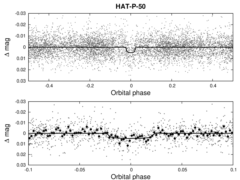
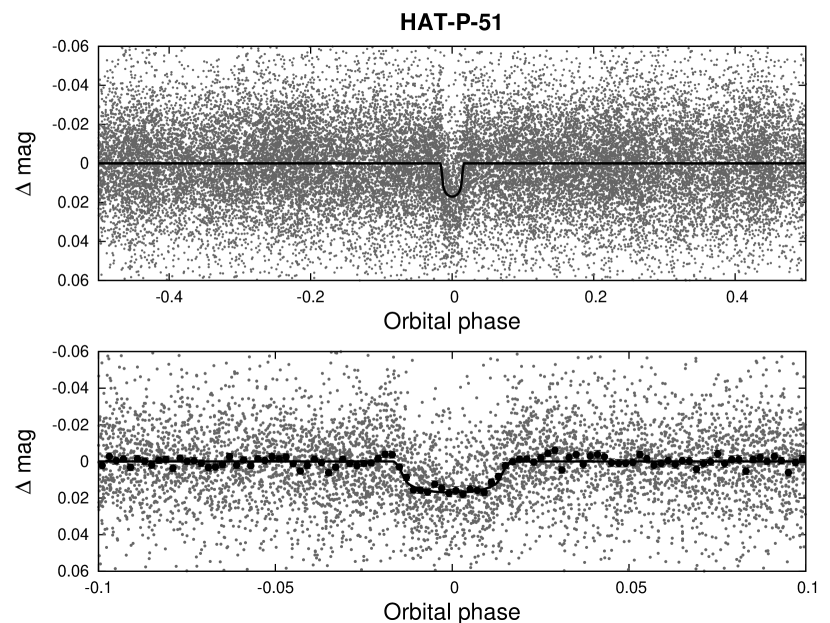
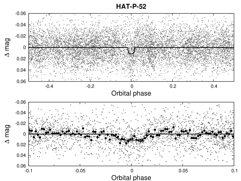
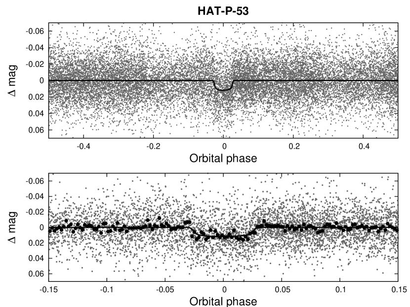
Figure 1.— Phase-folded unbinned HATNet light curves for HAT-P-50 (upper left), HAT-P-51 (upper right), HAT-P-52 (lower left), and HAT-P-53 (lower right). In each case we show two panels. The top panel shows the full light curve, while the bottom panel shows the light curve zoomed-in on the transit. The solid lines show the model fits to the light curves. The dark filled circles in the bottom panels show the light curves binned in phase with a bin size of 0.002.

Table 1 Summary of photometric observations

Instrument/Field	Date(s)	# Images	Cadence	Filter	Precision
			(sec)		(mmag)
HAT-P-50
HAT-10/G316	2008 Nov–2009 May	3214	352	Sloan $r$	7.5
HAT-5/G364	2009 May	21	411	Sloan $r$	10.6
HAT-9/G364	2008 Dec–2009 May	3159	352	Sloan $r$	7.5
BOS	2012 Feb 15	105	149	Sloan $i$	2.1
Keplercam	2012 Feb 18	443	54	Sloan $i$	1.2
BOS	2012 Feb 21	81	140	Sloan $i$	2.5
BOS	2012 Apr 08	61	143	Sloan $i$	1.6
Keplercam	2012 Nov 28	462	44	Sloan $i$	1.8
Keplercam	2012 Dec 23	277	45	Sloan $i$	2.3
Keplercam	2013 Jan 14	427	45	Sloan $i$	1.4
Keplercam	2013 Jan 17	380	45	Sloan $i$	1.6
HAT-P-51
HAT-6/G164	2007 Sep–2008 Feb	3652	349	Cousins $R$	30.3
HAT-9/G164	2007 Sep–2008 Feb	2767	349	Cousins $R$	25.9
HAT-10/G165	2010 Sep–2011 Jan	4215	230	Sloan $r$	24.3
HAT-5/G165	2010 Nov–2011 Feb	4142	354	Sloan $r$	24.1
HAT-8/G165	2010 Nov–2011 Feb	2240	238	Sloan $r$	23.6
HAT-6/G209	2010 Nov–2011 Feb	3794	351	Sloan $r$	18.4
HAT-9/G209	2010 Nov–2011 Feb	2151	352	Sloan $r$	18.0
HAT-7/G210	2010 Nov–2011 Jan	4047	229	Sloan $r$	19.1
Keplercam	2011 Oct 21	88	134	Sloan $i$	1.9
Keplercam	2012 Jan 05	92	133	Sloan $i$	2.7
Keplercam	2012 Oct 05	171	134	Sloan $i$	2.2
Keplercam	2012 Oct 26	137	134	Sloan $i$	2.6
Keplercam	2012 Nov 12	111	134	Sloan $i$	3.2
HAT-P-52
HAT-5/G212	2010 Sep–2010 Nov	2270	347	Sloan $r$	19.5
HAT-8/G212	2010 Aug–2010 Nov	5999	232	Sloan $r$	22.4
Keplercam	2010 Dec 23	101	134	Sloan $i$	2.0
Keplercam	2011 Sep 05	90	133	Sloan $i$	2.7
Keplercam	2011 Sep 27	188	134	Sloan $i$	2.3
Keplercam	2011 Nov 21	82	133	Sloan $i$	2.5
Keplercam	2012 Jan 07	64	194	Sloan $i$	3.0
HAT-P-53
HAT-6/G164	2007 Sep–2008 Feb	3653	349	Cousins $R$	26.4
HAT-9/G164	2007 Sep–2008 Feb	2764	349	Cousins $R$	24.5
HAT-10/G165	2010 Sep–2011 Jan	4234	230	Sloan $r$	19.3
HAT-5/G165	2010 Nov–2011 Feb	4134	354	Sloan $r$	19.4
HAT-8/G165	2010 Nov–2011 Feb	2240	238	Sloan $r$	20.4
Keplercam	2011 Oct 19	158	134	Sloan $i$	1.9
Keplercam	2011 Oct 27	381	73	Sloan $i$	2.5

2.2. Spectroscopic Observations

Follow-up spectroscopic observations were carried out using six different facilities. The aim of these observations was to aid in ruling out false positives, determine the atmospheric parameters of the host stars, and to confirm the planets by measuring the RV orbital variations induced by the transiting planets. The facilities used for each system are summarized in Table 2, and include the Tillinghast Reflector Echelle Spectrograph (TRES; Fűresz, 2008) on the 1.5 m Tillinghast Reflector at FLWO; the Astrophysical Research Consortium Echelle Spectrometer (ARCES; Wang et al., 2003) on the ARC 3.5 m telescope at Apache Point Observatory (APO) in New Mexico; the FIbre-fed Échelle Spectrograph (FIES) at the 2.5 m Nordic Optical Telescope (NOT) at La Palma, Spain (Djupvik & Andersen, 2010); the SOPHIE Spectrograph on the 1.93 m telescope at OHP (Bouchy et al., 2009) in France; HIRES (Vogt et al., 1994) on the Keck-I telescope in Hawaii together with the I₂ absorption cell; and the High-Dispersion Spectrograph (HDS; Noguchi et al., 2002) with the I₂ absorption cell (Kambe et al., 2002) on the Subaru telescope in Hawaii.

The TRES observations were used for reconnaissance (i.e. ruling out false positives with lower S/N spectra) for HAT-P-51, HAT-P-52 and HAT-P-53. For HAT-P-50 they were used both for reconnaissance and for measuring the orbital variation due to the planet. The raw echelle images were reduced to extracted spectra and analyzed to measure RVs and stellar atmospheric parameters following Buchhave et al. (2010). Observations of standard stars were made during each observing run and are used to correct the velocities from each run to the IAU system. Because these corrections are known for TRES, we adopt the TRES measurements for the systemic $\gamma$ velocity of each object listed in Table 4. The uncertainty on the absolute calibration is $\sim 0.1$ $\rm km\,s^{-1}$ and is dominated by the uncertainty in the absolute velocities of the standard stars.

The ARCES observations of HAT-P-51 and HAT-P-53 were used exclusively for reconnaissance (based on observations of standard stars the RV precision of this instrument is limited to $\sim 500$ $\rm m\,s^{-1}$). Observations were reduced to wavelength calibrated spectra using the echelle package in IRAF. For the wavelength calibration we made use of ThAr lamp spectra obtained before or after each science exposure, and with the same pointing as the science exposure. Each spectrum was analyzed to measure the RV of the star, its surface gravity, effective temperature, projected equatorial rotation velocity, and metallicity using the Stellar Parameter Classification (SPC; Buchhave et al., 2012) procedure, which cross-correlates the observed spectrum against a set of synthetic template spectra.

The single FIES spectrum obtained for HAT-P-51 was used for reconnaissance, and was reduced and analyzed following Buchhave et al. (2010).

SOPHIE observations of HAT-P-51 were collected in high-efficiency mode with the aim of confirming the planet by measuring the RV orbital wobble of its host star. The SOPHIE observations were reduced and analyzed following Boisse et al. (2013). Based on these observations we determined that HAT-P-51b is a Saturn-mass planet, and that the $\sim 40$ $\rm m\,s^{-1}$ precision of the SOPHIE observations for this object was insufficient to accurately determine the planetary mass. The precision in this case was limited due to significant contamination from scattered moon light, for uncontaminated spectra significantly higher precision may be obtained from the same S/N. We do not include these data in the analysis of HAT-P-51.

HDS observations were collected for HAT-P-50 and HAT-P-51 in order to confirm these TEP systems and characterize the planetary orbits. The observations were extracted and reduced to relative RVs in the solar system barycentric frame following Sato et al. (2002, 2012), while spectral line bisector spans (BSs) were computed following Torres et al. (2007).

HIRES observations were collected for HAT-P-51, HAT-P-52 and HAT-P-53. The observations have an RV precision of 5–10 $\rm m\,s^{-1}$ and are used here to characterize the orbital variations and to determine the stellar atmospheric parameters. The data were reduced to relative RVs in the barycentric frame following Butler et al. (1996). Spectral-line bisector spans (BSs) were computed following Torres et al. (2007), and $S$ activity indices were calculated following Isaacson & Fischer (2010). These were transformed to $\log_{10}R^{\prime}_{\rm HK}$ values following Noyes et al. (1984).

Based on the reconnaissance TRES, FIES and ARCES observations we find that none of the four targets shows evidence of being a composite system. All have radial velocity variations below 1 $\rm km\,s^{-1}$, and all are dwarf stars. The effective temperatures, projected rotation velocities, and surface gravities estimated from these spectra are consistent with the higher precision values presented in Table 4.

The high-precision RV measurements for all objects are seen to vary in phase with the transit ephemerides. These are shown in Figure 2. In this same figure we also show the phased BS measurements, which in all cases are consistent with no variation in phase with the ephemerides. The data are listed in Table 4 at the end of the paper.

Table 2 Summary of spectroscopy observations

Instrument	Date(s)	# Spec.	Res.	S/N Range	RV Precision
			$\Delta\lambda$/$\lambda$/1000		($\rm m\,s^{-1}$)
HAT-P-50
TRES	2010 Dec–2012 Feb	5	44	24.8–36.1	$116.0$
FIES	2012 Mar 13–17	5	67	31.0–69.9	$25.0$
HDS	2012 Feb 7	3	60	271–283	$\cdots$
HDS+I2	2012 Feb–2012 Sep	20	60	84–166	$23.0$
HAT-P-51
FIES	2011 Aug 4	1	46	27.4	$\cdots$
ARCES	2011 Sep 19	1	31.5	20.6	$\cdots$
TRES	2011 Sep 21	1	44	20.9	$\cdots$
SOPHIE	2011 Dec 4–12	4	39	23–28	$37$
HIRES	2011 Oct–Nov	2	55	83–94	$\cdots$
HIRES+I2	2011 Oct–2012 Feb	6	55	59–80	$5.4$
HDS	2012 Feb 9	4	60	52–56	$\cdots$
HDS+I2	2012 Feb 7–10	20	60	26–53	$9.2$
HAT-P-52
TRES	2010 Dec–2011 Jan	2	44	19.1–20.4	300
HIRES	2011 Oct 19	1	55	66	$\cdots$
HIRES+I2	2011 Feb–2012 Jul	7	55	26–59	$7.5$
HAT-P-53
TRES	2011 Sep 18–19	2	44	30.6–30.7	$80$
ARCES	2011 Sep 19–20	2	31.5	19.8–20.1	$380$
HIRES	2011 Nov 14	1	55	90	$\cdots$
HIRES+I2	2011 Nov–2012 Feb	6	55	62–79	$11.0$

Figure 2.— Phased high-precision RV measurements for HAT-P-50 (upper left), HAT-P-51 (upper right), HAT-P-52 (lower left), and HAT-P-53 (lower right). In each case we show three panels. The top panel shows the phased measurements together with our best-fit model (see Table 5) for each system. Zero-phase corresponds to the time of mid-transit. The center-of-mass velocity has been subtracted. The second panel shows the velocity $O\!-\!C$ residuals from the best fit. The error bars include the jitter terms listed in Table 5 added in quadrature to the formal errors for each instrument. The third panel shows the bisector spans (BS), with the mean value subtracted. The symbols used for each instrument are indicated in the top panel for each planet. Note the different vertical scales of the panels.

2.3. Photometric follow-up observations

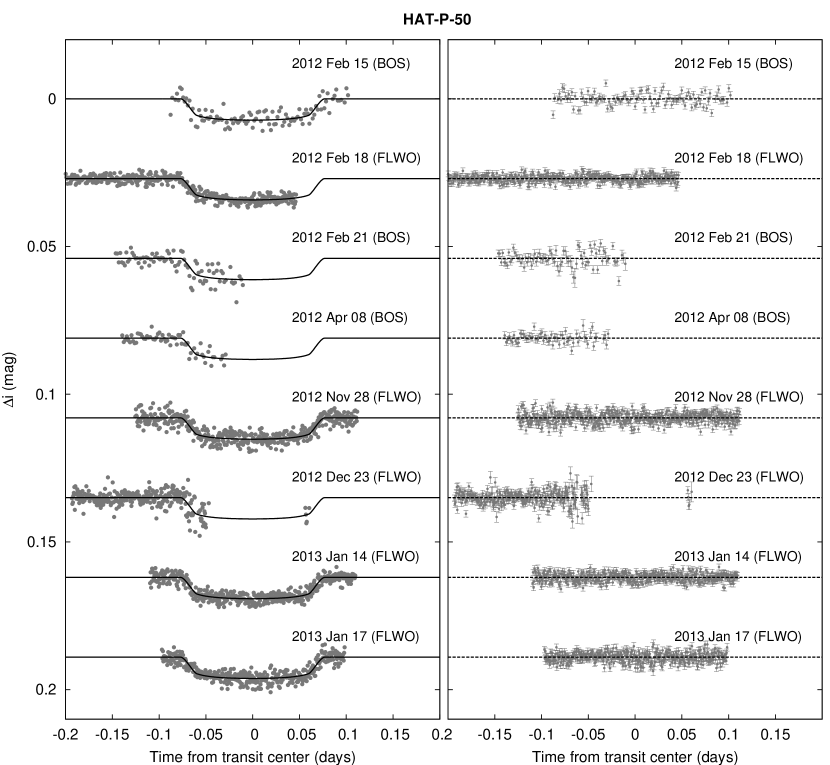
Figure 3.— Left: Unbinned transit light curves for HAT-P-50, acquired with the CCD imager on the BOS 0.8 m telescope, and Keplercam on the FLWO 1.2 m telescope. The light curves have been EPD and TFA processed, as described in § 3.3. The dates of the events and instruments used are indicated. Curves after the first are displaced vertically for clarity. Our best fit from the global modeling described in Section 3.3 is shown by the solid lines. Right: Residuals from the fits in the same order as the left panel. The error bars represent the photon and background shot noise, plus the readout noise.

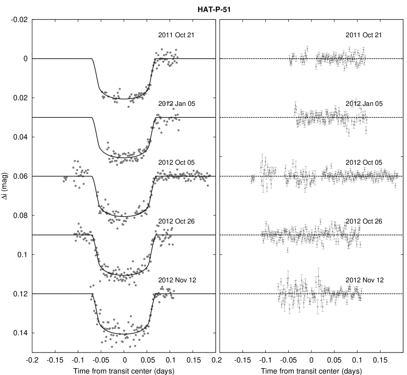
Figure 4.— Similar to Figure 3; here we show the follow-up light curves for HAT-P-51. All light curves were obtained with Keplercam on the FLWO 1.2 m telescope.

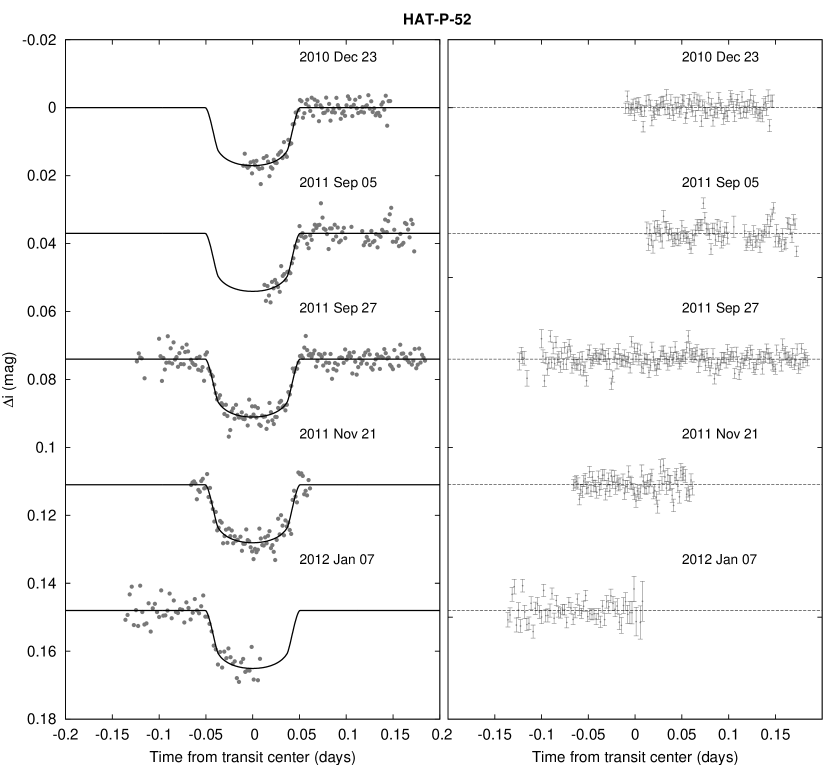
Figure 5.— Similar to Figure 3; here we show the follow-up light curves for HAT-P-52. All light curves were obtained with Keplercam on the FLWO 1.2 m telescope.

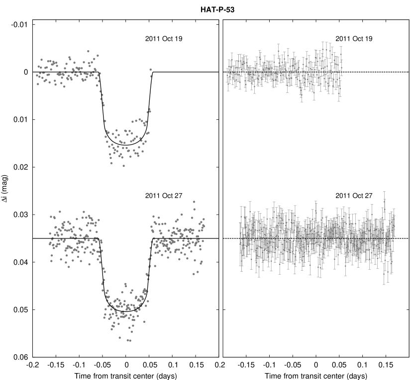
Figure 6.— Similar to Figure 3; here we show the follow-up light curves for HAT-P-53. All light curves were obtained with Keplercam on the FLWO 1.2 m telescope.

Additional time-series photometric measurements were obtained for all four of the systems using Keplercam on the FLWO 1.2 m telescope. These observations were carried out during the planetary transits to aid in ruling out blended eclipsing binary false positive scenarios, and to refine the light curve parameters (i.e. the orbital period, the planet to star radius ratio, the impact parameter and the transit duration). For HAT-P-50 we also obtained follow-up photometry with the CCD imager on the Byrne Observatory at Sedgwick (BOS) 0.8 m telescope, located at Sedgwick Reserve in Santa Ynez Valley, CA, and operated by the Las Cumbres Observatory Global Telescope institute (LCOGT; Brown et al., 2013). The events monitored with each instrument, together with the number of images obtained, the cadence, filter used and photometric precision are listed in Table 1.

We applied standard CCD calibration procedures to the Keplercam and BOS images and then reduced these to light curves using the aperture photometry methods described by Bakos et al. (2010). In doing this we made use of the stellar centroid positions measured directly from a set of registered and stacked frames rather than relying on catalog positions for astrometry as done in Bakos et al. (2010). All sources in the images, save the target TEP system, were used in performing the ensemble magnitude calibration. We corrected for additional systematic trends in the data by including the EPD and TFA noise filtering models in the fitting mentioned in Section 3.3. The resulting trend filtered light curves for HAT-P-50 through HAT-P-53 are shown in Figures 3–6, respectively. All photometric measurements made for the four objects are available in machine-readable form in Table 2.3.

Table 3 Light curve data for HAT-P-50–HAT-P-53.

Object	BJD	Mag	$\sigma_{\rm Mag}$	Mag(orig)	Filter	Instrument
	(2,400,000$+$)
HAT-P-50	$54863.83699$	$0.00928$	$0.00393$	$\cdots$	$r$	HATNet
HAT-P-50	$54935.64419$	$-0.00034$	$0.00517$	$\cdots$	$r$	HATNet
HAT-P-50	$54838.86248$	$0.00069$	$0.00443$	$\cdots$	$r$	HATNet
HAT-P-50	$54888.81494$	$-0.00915$	$0.00442$	$\cdots$	$r$	HATNet
HAT-P-50	$54792.03291$	$0.00668$	$0.00450$	$\cdots$	$r$	HATNet
HAT-P-50	$54910.67022$	$0.00400$	$0.00418$	$\cdots$	$r$	HATNet
HAT-P-50	$54863.84110$	$0.00001$	$0.00388$	$\cdots$	$r$	HATNet
HAT-P-50	$54935.64826$	$0.00737$	$0.00652$	$\cdots$	$r$	HATNet
HAT-P-50	$54838.86690$	$0.00070$	$0.00433$	$\cdots$	$r$	HATNet
HAT-P-50	$54888.81903$	$0.00426$	$0.00441$	$\cdots$	$r$	HATNet

Note. — This table is available in a machine-readable form in the online journal. A portion is shown here for guidance regarding its form and content.

3. Analysis

3.1. Properties of the parent star

The stellar atmospheric parameters that we adopted for the analysis, including the effective temperature $T_{\rm eff\star}$, the surface gravity $\log{g_{\star}}$, the metallicity $\rm[Fe/H]$ and the projected equatorial rotation velocity $v\sin{i}$, were determined for each system using SPC. For HAT-P-50 we applied this to the TRES and FIES spectra (applying to the individual spectra and adopting the average parameter values) while for the other three systems we used the Keck/HIRES I₂-free template spectra.

We used the Yonsei-Yale (Y2; Yi et al., 2001) theoretical stellar models to determine physical parameters of the stars, such as their masses, radii, luminosities and ages, based on the measured atmospheric parameters together with the bulk stellar densities $\rho_{\star}$ determined from our modelling of the light curves and RV measurements (Section 3.3). We generated a chain of $T_{\rm eff\star}$, $\rm[Fe/H]$ and $\rho_{\star}$ values for each object, where the $\rho_{\star}$ values are taken from the output of the MCMC procedure used to fit the light curves and RVs, while we assume uncorrelated Gaussian distributions for $T_{\rm eff\star}$ and $\rm[Fe/H]$. For each value in the chain we interpolate the Y2 models to find a combination of $M_{\star}$, age and $\rm[Fe/H]$ which matches the three input parameters (we assume solar-scaled abundances without $\alpha$-element enhancement). Combinations of $T_{\rm eff\star}$, $\rm[Fe/H]$ and $\rho_{\star}$ that do not match to a stellar model are rejected. In doing this we also reject the corresponding link in the LC+RV MCMC chain so that the final planetary parameters are restricted to regions of parameter space allowed by the stellar evolution models. The stellar models also provide other parameters such as $R_{\star}$ and $L_{\star}$ for a given $M_{\star}$, age and $\rm[Fe/H]$ combination. The result is a posterior chain of stellar parameters for each star. We use the chains to calculate the median and 68.3% confidence interval for each of the stellar parameters. These are listed in Table 4. We compare the measured $T_{\rm eff\star}$ and $\rho_{\star}$ values for each system to the model isochrones in Figure 7.

For HAT-P-50 and HAT-P-52 we found that the median $\log{g_{\star}}$ values determined from this procedure differed significantly from the values estimated from the spectra. For these stars we carried out a second iteration of SPC fixing $\log{g_{\star}}$ to the values determined from the stellar evolution modelling. We then performed a second iteration of the LC+RV modelling, with revised limb darkening parameters, followed by a second iteration of the stellar evolution modelling. The $\log{g_{\star}}$ values had converged after this iteration. For HAT-P-51 and HAT-P-53 a second iteration of SPC was not needed.

Distances are determined for each system by comparing the measured broad-band photometry listed in Table 4 to the magnitudes predicted in each filter by the models. We allow for extinction assuming a $R_{V}=3.1$ extinction law from Cardelli et al. (1989).

Based on this modelling we find that HAT-P-50 has a mass of $1.273_{-0.115}^{+0.049}$ $M_{\sun}$, a radius of $1.698\pm 0.071$ $R_{\sun}$, an age of $3.37_{-0.27}^{+1.44}$ Gyr, and is at a distance of $497\pm 21$ pc. HAT-P-51 has a mass of $0.976\pm 0.028$ $M_{\sun}$, a radius of $1.041_{-0.029}^{+0.038}$ $R_{\sun}$, an age of $8.2\pm 1.7$ Gyr, and is at a distance of $470\pm 16$ pc. HAT-P-52 has a mass of $0.887\pm 0.027$ $M_{\sun}$, a radius of $0.893\pm 0.047$ $R_{\sun}$, an age of $9.4\pm 4.1$ Gyr, and is at a distance of $385\pm 21$ pc. Finally, HAT-P-53 has a mass of $1.093\pm 0.043$ $M_{\sun}$, a radius of $1.209_{-0.062}^{+0.081}$ $R_{\sun}$, an age of $4.67_{-0.83}^{+1.45}$ Gyr, and is at a distance of $719\pm 43$ pc.

For HAT-P-51, -52 and -53 we used the Keck/HIRES spectra to determine median $\log_{10}R^{\prime}_{\rm HK}$ activity indices. We find that all three stars are inactive in the Ca II HK region, consistent with their slow rotation and lack of photometric variability.

Figure 7.— Model isochrones from Yi et al. (2001) for the measured metallicities of HAT-P-50 (upper left), HAT-P-51 (upper right), HAT-P-52 (lower left) and HAT-P-53 (lower right). In each case we show models for several different ages, with younger models being on the left and older ones on the right. For HAT-P-50, HAT-P-51 and HAT-P-52 we show ages of 0.2 Gyr and 1.0 to 14.0 Gyr in 1.0 Gyr increments. For HAT-P-53 we show ages of 0.2 Gyr and 1.0 to 9.0 Gyr in 1.0 Gyr increments. The adopted values of $T_{\rm eff\star}$ and $\rho_{\star}$ are shown together with their 1$\sigma$ and 2$\sigma$ confidence ellipsoids. The initial values of $T_{\rm eff\star}$ and $\rho_{\star}$ from the first SPC and light curve analyses are represented with a triangle for HAT-P-50 and HAT-P-52. Note the logarithmic vertical axes, and the different scales used in each panel.

Table 4 Stellar parameters for HAT-P-50–HAT-P-53

	HAT-P-50	HAT-P-51	HAT-P-52	HAT-P-53
Parameter	Value	Value	Value	Value	Source
Astrometric properties and cross-identifications
2MASS-ID	07521521+1208218	01241564+3248387	02505320+2901206	01272906+3858053
GSC-ID	GSC 0787-00340	GSC 2296-00637	GSC 1793-01136	GSC 2813-01266
R.A. (J2000)	$07^{\mathrm{h}}52^{\mathrm{m}}15.20{\mathrm{s}}$	$01^{\mathrm{h}}24^{\mathrm{m}}15.66{\mathrm{s}}$	$02^{\mathrm{h}}50^{\mathrm{m}}53.20{\mathrm{s}}$	$01^{\mathrm{h}}27^{\mathrm{m}}29.05{\mathrm{s}}$	2MASS
Dec. (J2000)	$+12{\arcdeg}08{\arcmin}21.9{\arcsec}$	$+32{\arcdeg}48{\arcmin}38.8{\arcsec}$	$+29{\arcdeg}01{\arcmin}20.6{\arcsec}$	$+38{\arcdeg}58{\arcmin}05.3{\arcsec}$	2MASS
$\mu_{\rm R.A.}$ ($\rm mas\,yr^{-1}$)	$10.20\pm 0.80$	$-9.8\pm 1.4$	$12.5\pm 2.1$	$-1.1\pm 1.8$	UCAC4
$\mu_{\rm Dec.}$ ($\rm mas\,yr^{-1}$)	$-4.6\pm 1.6$	$-16.8\pm 2.1$	$-24.7\pm 2.6$	$3.0\pm 2.2$	UCAC4
Spectroscopic properties
$T_{\rm eff\star}$ (K)	$6280\pm 49$	$5449\pm 50$	$5131\pm 50$	$5956\pm 50$	SPC
$\rm[Fe/H]$	$-0.180\pm 0.080$	$0.270\pm 0.080$	$0.280\pm 0.080$	$0.000\pm 0.080$	SPC
$v\sin{i}$ ($\rm km\,s^{-1}$)	$8.90\pm 0.50$	$1.70\pm 0.50$	$0.60\pm 0.50$	$4.10\pm 0.50$	SPC
$v_{\rm mac}$ ($\rm km\,s^{-1}$)	1.0	1.0	1.0	1.0	Assumed
$v_{\rm mic}$ ($\rm km\,s^{-1}$)	2.0	2.0	2.0	2.0	Assumed
$\gamma_{\rm RV}$ ($\rm km\,s^{-1}$)	$6.25\pm 0.10$	$-27.56\pm 0.10$	$61.50\pm 0.10$	$-16.99\pm 0.10$	TRES
$\log_{10}R^{\prime}_{\rm HK}$	$\cdots$	$-5.057\pm 0.050$	$-5.154\pm 0.089$	$-4.919\pm 0.042$	HIRES
Photometric properties
$B$ (mag)	$12.282\pm 0.050$	$14.261\pm 0.070$	$15.183\pm 0.050$	$\cdots$	APASS,TASS
$V$ (mag)	$11.762\pm 0.030$	$13.440\pm 0.040$	$14.068\pm 0.020$	$13.73\pm 0.18$	APASS,TASS
$I_{C}$ (mag)	$11.194\pm 0.052$	$12.67\pm 0.12$	$13.02\pm 0.17$	$13.13\pm 0.12$	TASS
$g$ (mag)	$11.973\pm 0.050$	$13.839\pm 0.050$	$14.631\pm 0.060$	$\cdots$	APASS
$r$ (mag)	$11.650\pm 0.030$	$13.194\pm 0.030$	$13.677\pm 0.080$	$\cdots$	APASS
$i$ (mag)	$11.550\pm 0.020$	$12.998\pm 0.040$	$13.441\pm 0.090$	$\cdots$	APASS
$J$ (mag)	$10.816\pm 0.021$	$12.039\pm 0.022$	$12.195\pm 0.022$	$12.468\pm 0.023$	2MASS
$H$ (mag)	$10.545\pm 0.020$	$11.645\pm 0.023$	$11.745\pm 0.022$	$12.202\pm 0.026$	2MASS
$K_{s}$ (mag)	$10.500\pm 0.018$	$11.614\pm 0.020$	$11.621\pm 0.021$	$12.100\pm 0.019$	2MASS
Derived properties
$M_{\star}$ ($M_{\sun}$)	$1.273_{-0.115}^{+0.049}$	$0.976\pm 0.028$	$0.887\pm 0.027$	$1.093\pm 0.043$	YY+$a/R_{\star}$+SPC
$R_{\star}$ ($R_{\sun}$)	$1.698\pm 0.071$	$1.041_{-0.029}^{+0.038}$	$0.893\pm 0.047$	$1.209_{-0.062}^{+0.081}$	YY+$a/R_{\star}$+SPC
$\log{g_{\star}}$ (cgs)	$4.072\pm 0.029$	$4.392\pm 0.027$	$4.483\pm 0.051$	$4.310\pm 0.043$	YY+$a/R_{\star}$+SPC
$\rho_{\star}$ ($\rm g\,cm^{-3}$)	$0.357\pm 0.037$	$1.223_{-0.135}^{+0.100}$	$1.75\pm 0.29$	$0.87\pm 0.13$	YY+$a/R_{\star}$+SPC
$L_{\star}$ ($L_{\sun}$)	$4.01\pm 0.38$	$0.859\pm 0.070$	$0.496\pm 0.060$	$1.65_{-0.18}^{+0.24}$	YY+$a/R_{\star}$+SPC
$M_{V}$ (mag)	$3.27\pm 0.11$	$5.055\pm 0.095$	$5.73\pm 0.13$	$4.27\pm 0.13$	YY+$a/R_{\star}$+SPC
$M_{K}$ (mag,ESO)	$2.052\pm 0.093$	$3.268\pm 0.071$	$3.69\pm 0.12$	$2.83\pm 0.12$	YY+$a/R_{\star}$+SPC
Age (Gyr)	$3.37_{-0.27}^{+1.44}$	$8.2\pm 1.7$	$9.4\pm 4.1$	$4.67_{-0.83}^{+1.45}$	YY+$a/R_{\star}$+SPC
$A_{V}$ (mag)	$0.011_{-0.011}^{+0.056}$	$0.012_{-0.012}^{+0.071}$	$0.412\pm 0.052$	$0.21\pm 0.14$	YY+$a/R_{\star}$+SPC
Distance (pc)	$497\pm 21$0	$470\pm 16$	$385\pm 21$	$719\pm 43$	YY+$a/R_{\star}$+SPC

3.2. Excluding blend scenarios

In order to exclude blend scenarios we carried out an analysis following (Hartman et al., 2012). We attempt to fit the available photometry (light curves, and catalog broad-band magnitudes calibrated to standard systems) for each object using a combination of three stars (two eclipsing, with a third diluting the eclipse signal) with properties taken from stellar evolution models.

For HAT-P-50, HAT-P-51 and HAT-P-53 we find that a model consisting of a planet transiting an isolated star provides a better (lower $\chi^{2}$) fit to the data than any of the blend models tested. For HAT-P-50 the best-fit blend model is excluded with $1.5\sigma$ confidence, while for both HAT-P-51 and HAT-P-53 it is excluded with $2\sigma$ confidence. We also simulated cross-correlation functions, RVs and BS measurements for the blend models tested, and found that any model that could plausibly fit the photometry for these systems (i.e. provides a fit that is no more than $5\sigma$ worse than the single star+planet model) would be easily identified as a composite stellar system based on the spectroscopy. We therefore conclude that all three of these objects are transiting planet systems.

Figure 8.— Phase-folded Keck/HIRES RVs for HAT-P-52 compared to the best-fit planetary orbit (dashed curve) and the best-fit RVs from a blended stellar eclipsing binary model (solid curve). This same blend model has BS variations that are below the observed scatter, and fits the photometric data, however it does not reproduce the form of the RV variation, which is well described by a transiting planet. The blend-model fit shown here consists of a $0.88$ $M_{\sun}$ foreground star blended with a $0.84$ $M_{\sun}$+$0.13$ $M_{\sun}$ eclipsing binary that has a distance modulus $0.35$ mag greater than the foreground star, and which has a $\gamma$ velocity that is $70$ $\rm km\,s^{-1}$ different from that of the foreground star. Reducing the difference in $\gamma$ velocities creates a more symmetric RV variation, but also results in the RV variation going to $0$ $\rm m\,s^{-1}$ at both phases 0.25 and 0.75. All other blend models simulated have RV variations that provide even poorer fits to the observations.

For HAT-P-52 we similarly find that the planet+star model provides a better fit to the data than any blend model tested, however the best-fit blend model differs by only $0.5\sigma$ from the planet+star model. We also find that there is a range of models consisting of a blend between a bright foreground star, and a background stellar eclipsing binary that is between $0.35$ mag and $4$ mag further in distance modulus than the foreground star, which cannot be ruled out based on the photometry or BS spans. For these models the simulated BS variations have a scatter that is below the 43 $\rm m\,s^{-1}$ scatter in the Keck/HIRES data, if we allow for a difference in the $\gamma$ velocities of the foreground star and background binary. We find, however, that similar to the case of HAT-P-49 (Bieryla et al., 2014), the expected form of the RV variations in these blends is significantly different from the observed sinusoidal variation, even though the overall amplitude of the variations is comparable (Fig. 8). We conclude that although the photometry and BS measurements for HAT-P-52 can be fit by a blended stellar eclipsing binary model, the RV observations cannot be.

While we can rule out the possibility that any of these objects is a blended stellar eclipsing binary system, we cannot rule out the possibility that one or more of these transiting planet systems also has a stellar companion. For HAT-P-50, we find that models including a faint companion with $M>0.6$ $M_{\sun}$ provide a slightly worse fit to the data than models without a companion. The difference in $\chi^{2}$ is small, however, and we can only rule out a stellar companion with $M>1.2$ $M_{\sun}$ at greater than $3\sigma$ confidence. For HAT-P-51, models with a companion having $M>0.5$ $M_{\sun}$have a slightly worse fit to the data, but we can only rule out companions with $M>0.95$ $M_{\sun}$ at greater than $3\sigma$ confidence. For HAT-P-52, companions with $M>0.35$ $M_{\sun}$ provide a slightly worse fit to the data, but all companions up to the mass of HAT-P-52 are permitted to within 3$\sigma$. For HAT-P-53 companions with $M>0.7$ $M_{\sun}$ provide a slightly worse fit, but all companions up to the mass of HAT-P-52 are permitted to within 3$\sigma$.

3.3. Global modeling of the data

We modeled the HATNet photometry, the follow-up photometry, and the high-precision RV measurements using the procedure described in detail by Pál et al. (2008) and Bakos et al. (2010) with modifications described by Hartman et al. (2012). This procedure makes use of the differential evolution Markov Chain Monte Carlo (DEMCMC) method (ter Braak, 2006; Eastman et al., 2013) to explore the fitness landscape and produce posterior parameter distributions. We allowed for RV jitter which we varied as a free parameter in the fit for each planet. We adopted independent jitters for each instrument as the methods for estimating the “formal” errors differ between reduction methods and instruments. For HIRES we made use of an empirical prior on the jitter as discussed in Hartman et al. (2014), while for the other instruments we used a Jeffreys prior (i.e. the prior probability for parameter $\sigma$ is $\propto 1/\sigma$). We fixed the limb darkening coefficients using the tabulation by Claret (2004) and the stellar atmospheric parameters given in Table 4.

The resulting parameters for each system are listed in Table 5. We find that HAT-P-50b is a hot Jupiter with a mass of $1.350\pm 0.073$ $M_{\rm J}$ and radius of $1.288\pm 0.064$ $R_{\rm J}$, HAT-P-51b is a hot Saturn with a mass of $0.309\pm 0.018$ $M_{\rm J}$ and radius of $1.293\pm 0.054$ $R_{\rm J}$, while HAT-P-52b and HAT-P-53b are hot Jupiters with masses of $0.818\pm 0.029$ $M_{\rm J}$ and $1.484\pm 0.056$ $M_{\rm J}$, and radii of $1.009\pm 0.072$ $R_{\rm J}$ and $1.318\pm 0.091$ $R_{\rm J}$, respectively. We fit all systems both allowing the eccentricity to vary and fixing it to zero. We find that all four systems are consistent with no eccentricity (the 95% confidence upper limits on the eccentricity when it is allowed to vary are $e<0.115$, $<0.123$, $<0.047$, and $<0.134$ for HAT-P-50b through HAT-P-53b, respectively). We therefore adopted the parameters for a fixed circular orbit in all cases.

Table 5Orbital and planetary parameters for HAT-P-50b–HAT-P-53b

	HAT-P-50b	HAT-P-51b	HAT-P-52b	HAT-P-53b
Parameter	Value	Value	Value	Value
Light curve parameters
$P$ (days)	$3.1220109\pm 0.0000065$	$4.2180278\pm 0.0000059$	$2.7535953\pm 0.0000094$	$1.9616241\pm 0.0000039$
$T_{c}$ (${\rm BJD}$)	$2456285.90993\pm 0.00036$	$2456194.12204\pm 0.00040$	$2455852.10326\pm 0.00041$	$2455829.44781\pm 0.00044$
$T_{14}$ (days)	$0.1531\pm 0.0011$	$0.1403\pm 0.0016$	$0.1003\pm 0.0017$	$0.1164\pm 0.0017$
$T_{12}=T_{34}$ (days)	$0.0176\pm 0.0013$	$0.0170\pm 0.0012$	$0.0130\pm 0.0018$	$0.0135\pm 0.0016$
$a/R_{\star}$	$5.68\pm 0.19$	$10.48_{-0.40}^{+0.28}$	$8.89\pm 0.49$	$5.61\pm 0.28$
$\zeta/R_{\star}$	$14.710\pm 0.077$0	$16.21\pm 0.12$0	$22.88\pm 0.27$0	$19.42\pm 0.17$0
$R_{p}/R_{\star}$	$0.0782\pm 0.0012$	$0.1278\pm 0.0020$	$0.1161\pm 0.0027$	$0.1120\pm 0.0019$
$b^{2}$	$0.395_{-0.050}^{+0.041}$	$0.077_{-0.052}^{+0.055}$	$0.213_{-0.098}^{+0.096}$	$0.142_{-0.090}^{+0.099}$
$b\equiv a\cos i/R_{\star}$	$0.629_{-0.041}^{+0.032}$	$0.277_{-0.119}^{+0.085}$	$0.461_{-0.122}^{+0.094}$	$0.38_{-0.15}^{+0.11}$
$i$ (deg)	$83.65\pm 0.57$0	$88.48\pm 0.57$0	$87.02\pm 0.86$0	$86.2\pm 1.5$0
Limb-darkening coefficients
$c_{1},i$ (linear term)	$0.1965$	$0.3348$	$0.3908$	$0.2387$
$c_{2},i$ (quadratic term)	$0.3570$	$0.2989$	$0.2628$	$0.3447$
RV parameters
$K$ ($\rm m\,s^{-1}$)	$161.3\pm 5.6$00	$39.5\pm 2.2$00	$128.4\pm 3.8$00	$226.8\pm 6.0$00
$e$	$<0.115$	$<0.123$	$<0.047$	$<0.134$
RV jitter HIRES ($\rm m\,s^{-1}$)	$\cdots$	$4.3\pm 1.2$	$5.2\pm 1.9$	$9.3\pm 3.2$
RV jitter HDS ($\rm m\,s^{-1}$)	$0.7\pm 7.1$	$0.0\pm 1.4$	$\cdots$	$\cdots$
RV jitter TRES ($\rm m\,s^{-1}$)	$68\pm 38$	$\cdots$	$\cdots$	$\cdots$
RV jitter FIES ($\rm m\,s^{-1}$)	$0.00\pm 0.91$	$\cdots$	$\cdots$	$\cdots$
Secondary eclipse parameters
$T_{s}$ (BJD)	$2456287.47093\pm 0.00036$	$2456196.23106\pm 0.00040$	$2455853.48006\pm 0.00041$	$2455830.42863\pm 0.00044$
$T_{s,14}$ (days)	$0.1531\pm 0.0011$	$0.1403\pm 0.0016$	$0.1003\pm 0.0017$	$0.1164\pm 0.0017$
$T_{s,12}$ (days)	$0.0176\pm 0.0013$	$0.0170\pm 0.0012$	$0.0130\pm 0.0018$	$0.0135\pm 0.0016$
Planetary parameters
$M_{p}$ ($M_{\rm J}$)	$1.350\pm 0.073$	$0.309\pm 0.018$	$0.818\pm 0.029$	$1.484\pm 0.056$
$R_{p}$ ($R_{\rm J}$)	$1.288\pm 0.064$	$1.293\pm 0.054$	$1.009\pm 0.072$	$1.318\pm 0.091$
$C(M_{p},R_{p})$	$0.48$	$-0.03$	$-0.15$	$0.34$
$\rho_{p}$ ($\rm g\,cm^{-3}$)	$0.78\pm 0.11$	$0.178\pm 0.024$	$0.98\pm 0.21$	$0.80\pm 0.15$
$\log g_{p}$ (cgs)	$3.302\pm 0.038$	$2.661_{-0.051}^{+0.037}$	$3.296\pm 0.065$	$3.325\pm 0.055$
$a$ (AU)	$0.04530_{-0.00140}^{+0.00058}$	$0.05069\pm 0.00049$	$0.03694\pm 0.00038$	$0.03159\pm 0.00042$
$T_{\rm eq}$ (K)	$1862\pm 34$	$1192\pm 21$	$1218\pm 37$	$1778\pm 48$
$\Theta$	$0.0751\pm 0.0044$	$0.0247\pm 0.0018$	$0.0673\pm 0.0050$	$0.0649\pm 0.0046$
$\log_{10}\langle F\rangle$ (cgs)	$9.433\pm 0.032$	$8.659\pm 0.031$	$8.696\pm 0.052$	$9.354\pm 0.046$

4. Discussion

In this paper we presented the discovery and characterization of four transiting exoplanets from the HATNet survey, including three hot Jupiters (HAT-P-50b, HAT-P-52b and HAT-P-53b) and a hot Saturn (HAT-P-51b). All four planets have masses and radii determined to better than 10% precision. The mass uncertainties are 5.4%, 5.8%, 3.5%, and 3.8% for HAT-P-50b through HAT-P-53b, respectively, while the respective radius uncertainties are 5.0%, 4.2%, 7.1%, and 6.9%. The stars HAT-P-50, -51, and -53 also have fairly precise isochrone-based age determinations (uncertainty less than 2 Gyr) thanks to their favorable position within the $T_{\rm eff}$–$\rho_{\star}$ plane (Fig. 7).

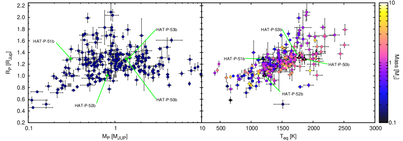
Figure 9.— Left: Mass–radius diagram for transiting planets with $0.1\,M_{\rm J}<M<10\,M_{\rm J}$. The four planets discovered here are indicated. The two filled gray squares show Saturn and Jupiter. The parameters for other transiting planets are compiled from the literature (c.f. %****␣hatp50-53.tex␣Line␣1475␣****http://www.exoplanets.org). Right: planet radius vs. estimated equilibrium temperature (assuming zero albedo and complete redistribution of heat) for the same sample of planets as shown at left. Symbols are assigned colors based on the planetary masses.

In Figure 9 we show the location of these planets on a mass–radius diagram, comparing them to the full sample of confirmed TEPs with $0.1<M_{p}<10$ $M_{\rm J}$. The new planets all fall within the range of values already seen by other planets, with HAT-P-51b falling near the upper envelope of the distribution of points in the mass–radius diagram, and HAT-P-52b falling near the lower envelope. We also show the location of each planet on a $T_{\rm eq}$–radius diagram. Again we find that the planets all follow the well-established trends. While not atypical compared to other known exoplanets, these objects contribute to the growing sample of well-characterized planets which may be used to explore the population of planets in the Galaxy through statistical methods.

In terms of potential for additional follow-up observations, we conclude that it should be feasible to measure the Rossiter-McLaughlin effect for HAT-P-50b, HAT-P-51b and HAT-P-53b using Subaru/HDS or Keck/HIRES. For HAT-P-50b the expected amplitude of the R-M effect is $42$ $\rm m\,s^{-1}$ for an aligned orbit (using eq. 40 in Winn, 2010). For HAT-P-51b the expected amplitude is $27$ $\rm m\,s^{-1}$, and for HAT-P-53b it is $48$ $\rm m\,s^{-1}$. The Subaru/HDS velocity residuals for HAT-P-50 have an RMS of 23 $\rm m\,s^{-1}$, with a median exposure time of 10 minutes. Assuming $20$ such exposures are obtained over the course of a single transit, it should be possible to measure the R-M amplitude to a precision of $5\sigma$ (based on fitting models to simulated observations). For HAT-P-51, the Keck/HIRES RVs have a residual RMS of $5.4$ $\rm m\,s^{-1}$, and a median exposure time of $25$ minutes. Seven of these exposures could be collected over a single transit, allowing a $9\sigma$ detection of the R-M amplitude. For HAT-P-53, the Keck/HIRES RVs have a residual of $11$ $\rm m\,s^{-1}$ and an exposure time of 25 minutes. For this system it should be possible to collect 6 similar exposures during a transit, and measure the R-M amplitude with $8\sigma$ confidence. For HAT-P-52b the R-M amplitude is only $\lesssim 7$ $\rm m\,s^{-1}$ (limited by the very slow rotation), and we would not expect to detect it in a single transit with better than 2$\sigma$ confidence.

The conclusion that the R-M effect should be easier to detect for both HAT-P-51 and HAT-P-53 than for HAT-P-50, despite both stars being significantly fainter than HAT-P-50, and despite both stars having a lower $v\sin{i}$, may be counter intuitive. The RV observations for HAT-P-51 and HAT-P-53 are both significantly higher precision than those for HAT-P-50, even though the HAT-P-50 observations have higher S/N. Some of the difference may be due to the different instruments (Subaru/HDS for HAT-P-50 vs. Keck/HIRES for HAT-P-51 and HAT-P-53). However, slower rotation and cooler surface temperatures are also factors which tend to improve the RV precision. In this respect we expect HAT-P-51 to have higher precision than HAT-P-53 at fixed S/N, and HAT-P-53 to have higher precision than HAT-P-50 at fixed S/N, which is what we see.

Measuring the R-M effect for HAT-P-51b may be of particular interest due to its small mass. HAT-P-11b and Kepler-63b are the only planets smaller than HAT-P-51b for which this effect has been measured to date (Winn et al., 2010 and Sanchis-Ojeda et al., 2013; the obliquity has also been measured for the Kepler-30 system by star-spot crossings, see Sanchis-Ojeda et al., 2012).

While the R-M effect should be detectable for HAT-P-50b, HAT-P-51b and HAT-P-53b, due to the relatively small value of $R_{p}/R_{\star}$ for HAT-P-50b, and the faintness of the other targets, none of the new planets are particularly well-suited for atmospheric characterization.

Table 6 Relative radial velocities, bisector spans, and activity index measurements for HAT-P-50–HAT-P-53.

$1853.80027$ $-42.75$ $2.53$ $-16.75$ $5.54$ $0.1550$ $0.317$ HIRES $1853.81798$  $\cdots$   $\cdots$  $-2.36$ $6.06$ $0.1300$ $0.322$ HIRES $1879.85898$  $\cdots$   $\cdots$  $10.56$ $6.81$ $0.1630$ $0.495$ HIRES $1879.87608$ $7.25$ $2.68$ $8.32$ $6.08$ $0.1570$ $0.499$ HIRES $1880.97599$ $42.01$ $2.48$ $9.54$ $5.32$ $0.0769$ $0.760$ HIRES $1903.95906$ $-35.87$ $2.63$ $-42.11$ $21.39$ $0.1550$ $0.209$ HIRES $1944.73569$ $24.93$ $2.55$ $-9.88$ $7.15$ $0.1170$ $0.876$ HIRES $1960.81411$ $31.81$ $3.23$ $5.14$ $7.02$ $0.1600$ $0.688$ HIRES $1964.71582$ $44.69$ $13.17$ $-0.33$ $26.24$  $\cdots$  $0.613$ HDS $1964.72359$ $27.51$ $11.37$ $-23.77$ $23.80$  $\cdots$  $0.615$ HDS $1964.73475$ $21.63$ $11.55$ $7.03$ $29.96$  $\cdots$  $0.617$ HDS $1964.74946$ $25.14$ $9.83$ $3.26$ $34.15$  $\cdots$  $0.621$ HDS $1964.76417$ $33.95$ $9.59$ $0.65$ $35.27$  $\cdots$  $0.624$ HDS $1965.71533$ $32.14$ $15.07$ $-2.89$ $24.12$  $\cdots$  $0.850$ HDS $1965.73005$ $29.21$ $12.47$ $9.32$ $36.71$  $\cdots$  $0.853$ HDS $1965.74477$ $33.24$ $11.95$ $-14.30$ $27.64$  $\cdots$  $0.857$ HDS $1965.75948$ $34.67$ $14.11$ $-16.82$ $27.55$  $\cdots$  $0.860$ HDS $1965.77418$ $13.59$ $12.75$ $21.67$ $22.10$  $\cdots$  $0.864$ HDS $1965.78890$ $15.87$ $21.41$ $23.88$ $25.83$  $\cdots$  $0.866$ HDS $1966.72018$  $\cdots$   $\cdots$  $-4.21$ $31.52$  $\cdots$  $0.088$ HDS $1966.73489$  $\cdots$   $\cdots$  $9.59$ $32.96$  $\cdots$  $0.092$ HDS $1966.74959$  $\cdots$   $\cdots$  $4.25$ $32.50$  $\cdots$  $0.095$ HDS $1966.76429$  $\cdots$   $\cdots$  $5.05$ $34.50$  $\cdots$  $0.099$ HDS $1966.77907$ $-12.89$ $12.16$ $-0.33$ $34.37$  $\cdots$  $0.102$ HDS $1966.79377$ $-33.08$ $11.65$ $27.17$ $29.63$  $\cdots$  $0.106$ HDS $1966.80848$ $-13.58$ $15.24$ $5.11$ $13.87$  $\cdots$  $0.109$ HDS $1967.72003$ $-24.46$ $14.33$ $-2.79$ $22.98$  $\cdots$  $0.325$ HDS $1967.73475$ $-48.37$ $13.90$ $-12.59$ $23.40$  $\cdots$  $0.329$ HDS $1967.74946$ $-42.32$ $13.39$ $-11.16$ $21.89$  $\cdots$  $0.332$ HDS $1967.76417$ $-34.03$ $12.75$ $0.39$ $20.57$  $\cdots$  $0.336$ HDS $1967.77888$ $-28.16$ $13.62$ $3.97$ $17.43$  $\cdots$  $0.339$ HDS $1967.79359$ $-28.23$ $14.33$ $-32.17$ $31.51$  $\cdots$  $0.343$ HDS    HAT-P-52    $1611.81789$ $134.02$ $4.23$ $17.97$ $81.51$ $0.2500$ $0.738$ HIRES $1853.86184$ $90.96$ $3.67$ $-6.05$ $13.12$ $0.1870$ $0.639$ HIRES $1853.88098$  $\cdots$   $\cdots$  $67.06$ $32.55$ $0.1230$ $0.646$ HIRES $1879.90065$ $-62.91$ $4.21$ $-11.44$ $32.23$ $0.1220$ $0.095$ HIRES $1880.99970$ $1.46$ $3.24$ $10.18$ $16.84$ $0.1500$ $0.494$ HIRES $1882.08871$ $76.62$ $7.72$ $-77.06$ $46.76$ $0.4450$ $0.890$ HIRES $1972.84557$ $102.30$ $4.25$  $\cdots$   $\cdots$   $\cdots$  $0.849$ HIRES $2139.06062$ $-134.45$ $3.86$ $-0.66$ $15.61$ $0.1360$ $0.212$ HIRES    HAT-P-53    $1877.91488$ $217.41$ $4.13$ $3.37$ $8.66$ $0.1820$ $0.708$ HIRES $1879.81971$ $220.06$ $3.91$ $-8.64$ $5.38$ $0.1710$ $0.679$ HIRES $1879.83898$  $\cdots$   $\cdots$  $-6.30$ $5.05$ $0.1700$ $0.689$ HIRES $1880.95723$ $-228.59$ $3.82$ $4.64$ $4.22$ $0.1740$ $0.259$ HIRES $1944.84748$ $187.44$ $5.04$ $11.55$ $4.67$ $0.1010$ $0.829$ HIRES $1960.79667$ $43.84$ $4.68$ $-10.07$ $13.55$ $0.1430$ $0.959$ HIRES $1972.75173$ $-68.38$ $4.23$ $-14.42$ $7.85$ $0.1570$ $0.054$ HIRES

Note. — Note that for the iodine-free template exposures we do not measure the RV but do measure the BS and S index. Such template exposures can be distinguished by the missing RV value.

References

- Alonso et al. (2004) Alonso, R., Brown, T. M., Torres, G., et al. 2004, ApJ, 613, L153
- Bakos et al. (2004) Bakos, G., Noyes, R. W., Kovács, G., et al. 2004, PASP, 116, 266
- Bakos et al. (2010) Bakos, G. Á., Torres, G., Pál, A., et al. 2010, ApJ, 710, 1724
- Bakos et al. (2013) Bakos, G. Á., Csubry, Z., Penev, K., et al. 2013, PASP, 125, 154
- Béky et al. (2011) Béky, B., Bakos, G. Á., Hartman, J., et al. 2011, ApJ, 734, 109
- Bieryla et al. (2014) Bieryla, A., Hartman, J. D., Bakos, G. Á., et al. 2014, AJ, 147, 84
- Boisse et al. (2013) Boisse, I., Hartman, J. D., Bakos, G. Á., et al. 2013, A&A, 558, A86
- Bouchy et al. (2009) Bouchy, F., Hébrard, G., Udry, S., et al. 2009, A&A, 505, 853
- Brown et al. (2013) Brown, T. M., Baliber, N., Bianco, F. B., et al. 2013, PASP, 125, 1031
- Buchhave et al. (2010) Buchhave, L. A., Bakos, G. Á., Hartman, J. D., et al. 2010, ApJ, 720, 1118
- Buchhave et al. (2012) Buchhave, L. A., Latham, D. W., Johansen, A., et al. 2012, Nature, 486, 375
- Burrows et al. (2007) Burrows, A., Hubeny, I., Budaj, J., & Hubbard, W. B. 2007, ApJ, 661, 502
- Butler et al. (1996) Butler, R. P., Marcy, G. W., Williams, E., et al. 1996, PASP, 108, 500
- Cardelli et al. (1989) Cardelli, J. A., Clayton, G. C., & Mathis, J. S. 1989, ApJ, 345, 245
- Charbonneau et al. (2002) Charbonneau, D., Brown, T. M., Noyes, R. W., & Gilliland, R. L. 2002, ApJ, 568, 377
- Claret (2004) Claret, A. 2004, A&A, 428, 1001
- Dawson & Johnson (2012) Dawson, R. I., & Johnson, J. A. 2012, ApJ, 756, 122
- Deeming (1975) Deeming, T. J. 1975, Ap&SS, 36, 137
- Djupvik & Andersen (2010) Djupvik, A. A., & Andersen, J. 2010, in Highlights of Spanish Astrophysics V, ed. J. M. Diego, L. J. Goicoechea, J. I. González-Serrano, & J. Gorgas, 211
- Droege et al. (2006) Droege, T. F., Richmond, M. W., Sallman, M. P., & Creager, R. P. 2006, PASP, 118, 1666
- Eastman et al. (2013) Eastman, J., Gaudi, B. S., & Agol, E. 2013, PASP, 125, 83
- Enoch et al. (2012) Enoch, B., Collier Cameron, A., & Horne, K. 2012, A&A, 540, A99
- Fűresz (2008) Fűresz, G. 2008, PhD thesis, Univ. of Szeged, Hungary
- Guillot et al. (2006) Guillot, T., Santos, N. C., Pont, F., et al. 2006, A&A, 453, L21
- Hansen & Barman (2007) Hansen, B. M. S., & Barman, T. 2007, ApJ, 671, 861
- Hartman et al. (2012) Hartman, J. D., Bakos, G. Á., Béky, B., et al. 2012, AJ, 144, 139
- Hartman et al. (2014) Hartman, J. D., Bakos, G. Á., Torres, G., et al. 2014, AJ, 147, 128
- Isaacson & Fischer (2010) Isaacson, H., & Fischer, D. 2010, ApJ, 725, 875
- Kambe et al. (2002) Kambe, E., Sato, B., Takeda, Y., et al. 2002, PASJ, 54, 865
- Kovács et al. (2005) Kovács, G., Bakos, G., & Noyes, R. W. 2005, MNRAS, 356, 557
- Kovács et al. (2002) Kovács, G., Zucker, S., & Mazeh, T. 2002, A&A, 391, 369
- Kurtz (1985) Kurtz, D. W. 1985, MNRAS, 213, 773
- Latham et al. (2009) Latham, D. W., Bakos, G. Á., Torres, G., et al. 2009, ApJ, 704, 1107
- Laughlin et al. (2011) Laughlin, G., Crismani, M., & Adams, F. C. 2011, ApJ, 729, L7
- McCullough et al. (2005) McCullough, P. R., Stys, J. E., Valenti, J. A., et al. 2005, PASP, 117, 783
- Mullally et al. (2015) Mullally, F., Coughlin, J. L., Thompson, S. E., et al. 2015, ArXiv e-prints, 1502.02038
- Noguchi et al. (2002) Noguchi, K., Aoki, W., Kawanomoto, S., et al. 2002, PASJ, 54, 855
- Noyes et al. (1984) Noyes, R. W., Hartmann, L. W., Baliunas, S. L., Duncan, D. K., & Vaughan, A. H. 1984, ApJ, 279, 763
- Pál (2009) Pál, A. 2009, PhD thesis, Department of Astronomy, Eötvös Loránd University
- Pál et al. (2008) Pál, A., Bakos, G. Á., Torres, G., et al. 2008, ApJ, 680, 1450
- Pepper et al. (2007) Pepper, J., Pogge, R. W., DePoy, D. L., et al. 2007, PASP, 119, 923
- Pollacco et al. (2006) Pollacco, D. L., Skillen, I., Collier Cameron, A., et al. 2006, PASP, 118, 1407
- Queloz et al. (2000) Queloz, D., Eggenberger, A., Mayor, M., et al. 2000, A&A, 359, L13
- Sanchis-Ojeda et al. (2012) Sanchis-Ojeda, R., Fabrycky, D. C., Winn, J. N., et al. 2012, Nature, 487, 449
- Sanchis-Ojeda et al. (2013) Sanchis-Ojeda, R., Winn, J. N., Marcy, G. W., et al. 2013, ApJ, 775, 54
- Sato et al. (2002) Sato, B., Kambe, E., Takeda, Y., Izumiura, H., & Ando, H. 2002, PASJ, 54, 873
- Sato et al. (2012) Sato, B., Hartman, J. D., Bakos, G. Á., et al. 2012, PASJ, 64, 97
- ter Braak (2006) ter Braak, C. J. F. 2006, Statistics and Computing, 16, 239
- Torres et al. (2007) Torres, G., Bakos, G. Á., Kovács, G., et al. 2007, ApJ, 666, L121
- Vogt et al. (1994) Vogt, S. S., Allen, S. L., Bigelow, B. C., et al. 1994, in Society of Photo-Optical Instrumentation Engineers (SPIE) Conference Series, Vol. 2198, Society of Photo-Optical Instrumentation Engineers (SPIE) Conference Series, ed. D. L. Crawford & E. R. Craine, 362
- Wang et al. (2003) Wang, S.-i., Hildebrand, R. H., Hobbs, L. M., et al. 2003, in Society of Photo-Optical Instrumentation Engineers (SPIE) Conference Series, Vol. 4841, Instrument Design and Performance for Optical/Infrared Ground-based Telescopes, ed. M. Iye & A. F. M. Moorwood, 1145–1156
- Winn (2010) Winn, J. N. 2010, ArXiv e-prints, 1001.2010
- Winn et al. (2010) Winn, J. N., Johnson, J. A., Howard, A. W., et al. 2010, ApJ, 723, L223
- Yi et al. (2001) Yi, S., Demarque, P., Kim, Y.-C., et al. 2001, ApJS, 136, 417
- Zacharias et al. (2012) Zacharias, N., Finch, C. T., Girard, T. M., et al. 2012, VizieR Online Data Catalog, 1322, 0