Image patch analysis of sunspots and active regions. I. Intrinsic dimension and correlation analysis

Abstract

The flare-productivity of an active region is observed to be related to its spatial complexity. Mount Wilson or McIntosh sunspot classifications measure such complexity but in a categorical way, and may therefore not use all the information present in the observations. Moreover, such categorical schemes hinder a systematic study of an active region’s evolution for example.

We propose fine-scale quantitative descriptors for an active region’s complexity and relate them to the Mount Wilson classification. We analyze the local correlation structure within continuum and magnetogram data, as well as the cross-correlation between continuum and magnetogram data. We compute the intrinsic dimension, partial correlation and canonical correlation analysis (CCA) of image patches of continuum and magnetogram active region images taken from the SOHO-MDI instrument. We use masks of sunspots derived from continuum as well as larger masks of magnetic active regions derived from magnetogram to analyze separately the core part of an active region from its surrounding part. We find relationships between the complexity of an active region as measured by its Mount Wilson classification and the intrinsic dimension of its image patches. Partial correlation patterns exhibit approximately a third-order Markov structure. CCA reveals different patterns of correlation between continuum and magnetogram within the sunspots and in the region surrounding the sunspots. Intrinsic dimension has the potential to distinguish simple from complex active regions. These results also pave the way for patch-based dictionary learning with a view towards automatic clustering of active regions.

1 Introduction

Active regions (AR) in the solar atmosphere have intense and intricate magnetic fields that emerge from subsurface layers to form loops which extend into the corona. When active regions undergo external forcing such as flux emergence and rearrangement, the system may destabilize. The stored magnetic energy is then suddenly released as accelerated particles (electrons, protons, ions) and an increase in radiation called a flare is observed across the entire electromagnetic spectrum (Phillips, 1991).

The morphology of sunspots is correlated with flare occurrence and has therefore received a lot of attention. The Mount Wilson classification scheme (Hale et al., 1919) groups sunspots into four main classes based on the magnetic structure, that is, on the relative locations and sizes of concentrations of opposite polarity magnetic flux. The sunspots with simplest morphology belong to the unipolar $\alpha$ and the bipolar $\beta$ groups. More complex morphologies are described as $\beta\gamma$ when a bipolar sunspot is such that a single north-south polarity inversion line cannot divide the two polarities. When a $\beta\gamma$ sunspot group contains in addition a $\delta$ spot, that is, umbrae of different polarities inside a single penumbra, it is labeled as a $\beta\gamma\delta$ group. The presence of a $\delta$ configuration, where large values of opposite polarity exist close together, was identified as a warning of the build up of magnetic energy stress with an increased probability of a large flare (Mayfield and Lawrence, 1985; Sammis et al., 2000). McIntosh (1990) proposes another classification scheme containing 60 classes, thus describing the magnetic structure in greater details. The McIntosh classification is the basis for several flare forecasting methods which estimate the flare occurrence rate from historical records of flares and active region classes (Bornmann and Shaw, 1994), possibly combining such information with observed waiting time distribution between flares (Gallagher et al., 2002; Bloomfield et al., 2012).

The McIntosh and Mount Wilson classifications are in general carried out manually, and this results in inconsistencies that stem from human observation bias as well as non-reproducible catalogs. To overcome these caveats, some supervised machine learning methods have been proposed to automatically classify sunspot groups according to these schemes. Stenning et al. (2013) extract various measurements from continuum and magnetogram images, and then feed these into a machine learning classifier which reproduces the Mount Wilson classification. Colak and Qahwaji (2008) employ neural networks and supervised classification techniques to reproduce the McIntosh scheme and use those results in a flare forecasting system (Colak and Qahwaji, 2009). While these approaches reduce the human bias, they do not use the information present in sunspot images in an optimal way and make the study of AR dynamic behavior impractical.

Several attempts were made to find quantitative descriptors of an active region’s complexity. McAteer et al. (2005) showed that fractal dimension of an active region alone cannot distinguish between the various Mount Wilson classes. The generalization to multifractal spectrum, where each scale has its own fractal dimension, allowed to study in greater details the evolution of active region in view of distinguishing between quiet and flare-productive active regions. Box counting methods (Georgoulis, 2005; Abramenko, 2005; Conlon et al., 2008) as well as more accurate methods based on continuous wavelet transform (Kestener et al., 2010; Conlon et al., 2010) were employed. Continuous wavelet transforms and energy spectrum were also used with a similar purpose in Hewett et al. (2008); McAteer et al. (2010).

Wavelet basis functions act as a microscope to describe local discontinuities and gradients in an image, and Ireland et al. (2008) used two multiresolution analyses to compute at various length scales the gradients of the magnetic field along lines separating opposite polarities. Using a data set of about 10 000 magnetogram images, they showed that, at all length scales, those gradients increase going from $\alpha$ to $\beta$, $\beta\gamma$, and $\beta\gamma\delta$ classes.

However, a wavelet analysis is known to generate artifacts due to the particular shape of the specific wavelet functions. Signal representations based on a set of redundant functions called a dictionary, were therefore introduced (Mallat and Zhang, 1993). Elad and Aharon (2006) proposed the use of a small sized dictionary to find a sparse representation of patches. Specifically, a patch is a $m\times m$-pixel neighborhood, and a patch analysis of a $n$-pixel image will process the $m^{2}\times n$ data matrix that collects the overlapping patches. See Figure 1 for a representation.

As an example of image patch analysis, Elad and Aharon (2006) considered the problem of denoising an image corrupted by additive Gaussian noise. They computed a sparse representation of patches over a dictionary, thus effectively denoising the patches. The dictionary itself may either be fixed a priori or learned from the corrupted patches. An estimate of the noise-free image is then obtained by averaging the denoised overlapping patches. Elad and Aharon (2006) showed that dictionary learning methods based on patch analysis are more flexible and provide superior results in the context of image denoising.

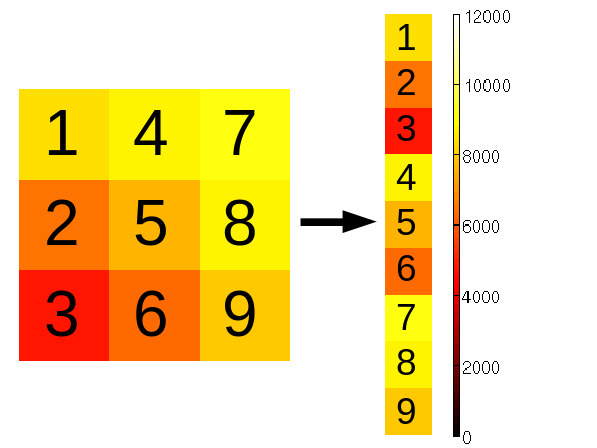
Figure 1: An example patch from the edge of a sunspot in a continuum image and its column representation.

In this paper, we carry out a patch analysis of a set of sunspots and active region magnetogram images that span the four main Mount Wilson classes. We estimate the intrinsic dimension of the local patches, and show how it relates to the Mount Wilson classification. We also study patterns of local correlation using partial correlation and canonical correlation analysis, which reveal some characteristics of simple and more complex active regions. Such analysis also serves as a preparation to an unsupervised clustering of active region using patch-based dictionary learning which will be presented in a companion paper (Moon et al., 2015).

Section 2 describes our data set. Unlike previous works, our approach combines information from two modalities: photospheric continuum images and magnetograms, both obtained by the Michelson Doppler Imager (MDI) on board the Solar and Heliospheric Observatory (SOHO) spacecraft. We consider 424 active regions spanning the four main Mount Wilson classes. We use SMART masks (Higgins et al., 2011) to delineate the boundaries of magnetic active regions, and the STARA algorithm (Watson et al., 2011) which provides masks for umbrae and penumbrae from the continuum images. These two masks enable us to differentiate between pixels belonging to the actual sunspots and pixels featuring the region surrounding the sunspots.

In Section 3, the intrinsic dimension of the image patches extracted from the two modalities is estimated using both linear and non-linear methods. The linear method relies on Principal Component Analysis (PCA) (Jolliffe, 2002), while the non-linear method relies on a $k$-Nearest Neighbor graph approach (Costa and Hero III, 2006; Carter et al., 2010). The latter method also estimates the local intrinsic dimension, which has several advantages over a global estimate. We show that the intrinsic dimension is related to the complexity of the sunspot groups.

Section 4 identifies the spatial and modal interactions of the patches at different scales by estimating the partial correlation and by using canonical correlation analysis (CCA) (Muller, 1982; Nimon et al., 2010). This gives insight about relationships that may exist between active region complexity and the correlation patterns.

This paper expands and refines some of the work in Moon et al. (2014). Whereas Moon et al. (2014) used fixed size square pixel regions centered on the sunspot group as input to the analyses, in this paper SMART detection masks are used. A larger set of images is considered in all methods which enables us to analyze the relationships of intrinsic dimension and correlation with AR complexity. We also explore the partial correlation of patches which was not included in Moon et al. (2014).

2 Data

The data used in this study are taken from the Michelson Doppler Imager (MDI) instrument (Scherrer et al., 1995) on board the SOHO Spacecraft.

Within the time range of 1996-2010, we select a set of 424 ARs as follows. Using the information from the Solar Region Summary reports compiled by the Space Weather Prediction Center of NOAA http://www.swpc.noaa.gov/ftpdir/forecasts/SRS/, we consider ARs located within $30^{\circ}$ of the solar meridian. We looked at a maximum of two-hundred instances per Mount Wilson types $\alpha,\beta,\beta\gamma,$ and $\beta\gamma\delta$. Out of this first selection, we removed AR with a longitudinal extent smaller than four degrees, and finally we checked if MDI continuum and magnetogram data were available. This provides us with a number of ARs in each Mount Wilson class as given by Table 1. In our analysis, we also divide the ARs into two groups: simple ARs ($\alpha$ and $\beta$) and complex ARs ($\beta\gamma$ and $\beta\gamma\delta$).

Table 1: Number of each AR per Mt. Wilson class. Simple ARs include $\alpha$ and $\beta$ groups while complex ARs are $\beta\gamma$ and $\beta\gamma\delta$ groups.

	$\alpha$	$\beta$	$\beta\gamma$	$\beta\gamma\delta$	Simple	Complex	Total
Number of AR	50	192	130	52	242	182	424

AR are observed using two modalities: photospheric continuum images and magnetogram. SOHO-MDI provides almost continuous observations of the Sun in the white-light continuum, in the vicinity of the Ni i 676.78 nm photospheric absorption line. These photospheric intensity images are primarily used for sunspot observations. MDI data are available in several processed “levels”. We use level-1.8 images, and rotate them with North up. SOHO provides two to four MDI photospheric intensity images per day with continuous coverage since 1995. We also use the level-1.8 line-of-sight (LOS) MDI magnetograms, recorded with a nominal cadence of 96 minutes. The magnetograms show the magnetic fields of the solar photosphere, with negative (represented as black) and positive (as white) areas indicating opposite LOS magnetic-field orientations.

As stated in Section 1, SMART masks (Higgins et al., 2011) are used to determine the boundaries of magnetic active regions from MDI magnetograms. Those masks are applied also on continuum images to determine the surrounding part of the sunspot that is affected by magnetic fragments as seen in magnetogram images. Similarly, the STARA algorithm (Watson et al., 2011) provides masks for sunspots (umbrae and penumbrae) from MDI continuum and those masks are applied on magnetogram images to determine the AR cores corresponding to the sunspots. Combining these two types of masks provides thus two sets of pixels within each AR: those belonging to the sunspots themselves as found by STARA and those belonging to the magnetic fragments (or background) within an AR as found by the difference set between the SMART and STARA masks.

As in Moon et al. (2014) we use image patch features to account for spatial dependencies using square patches of pixels. Thus if a SMART mask of an image has $n$ pixels and we use a $m\times m$ patch, the corresponding continuum data matrix $\mathbf{X}$ is $m^{2}\times n$ where the $i$th column contains the pixels in the patch centered at the $i$th pixel. The magnetogram data matrix $\mathbf{Y}$ is formed in the same way and the full data matrix is $\mathbf{Z}=\left(\begin{array}[]{c}\mathbf{X}\\ \mathbf{Y}\end{array}\right)$ with size $2m^{2}\times n$. We let $\mathbf{z}_{i}$ denote the $i$th column of $\mathbf{Z}$. The images from both modalities are also normalized prior to analyzing them.

In image patch analysis, the size of the patch should be no larger than the smallest feature that is to be captured. Otherwise, the relevant feature may be suppressed. Additionally, large patches lead to high-dimensional estimates which suffer in accuracy from "the curse of dimensionality," which refers to the fact that the number of observations must increase at least linearly in the number of parameters for accurate estimates to be possible in statistical inference (Bühlmann and Van De Geer, 2011). Since some sunspot and active region features can be quite small and to limit the effects of high dimensionality on our analysis, we primarily use $3\times 3$ patches in each modality although larger patches are used in Section 4 when analyzing spatial correlations in the images.

3 Intrinsic Dimension Estimation

The goal of this section is to determine the number of intrinsic parameters or degrees of freedom required to describe the spatial and modal dependencies using image patches. We consider $3\times 3$ patches within both the continuum and magnetogram images giving an extrinsic dimension of 18. The intrinsic dimension will determine how redundant these 18 dimensions are. In addition, intrinsic dimension provides an indicator of complexity which we compare against the Mount Wilson classification, similarly to what McAteer et al. (2005) and Ireland et al. (2008) did using fractal dimension and gradient strength along polarity separating lines, respectively. More details on the concept of intrinsic dimension on manifolds are included in Appendix A.1.

It is also important to know whether linear analyses can be accurately applied to the data or whether non-linear techniques are required. Linear methods have been applied successfully to solar images before such as in Dudok de Wit et al. (2013). However, it is not guaranteed that natural images are best represented using linear methods as there are cases where non-linear models have superior performance (Dobigeon et al., 2014). Thus this is important to investigate both for further analysis of the data as in Moon et al. (2015) and for the correlation analysis in Section 4. If the data lie on a nonlinear subspace and we perform a linear analysis of the data (e.g. partial correlation, canonical correlation analysis, or principal component analysis), then the results will be only a linear approximation of the true relationships and dependencies of the data. Nonlinear methods of analysis would be necessary to obtain higher accuracy in this case. To answer this question, we estimate the local intrinsic dimension using a method appropriate for linear subspaces and a method appropriate for any (linear or non-linear) smooth subspace and then compare the results.

3.1 PCA: A Linear Estimator

Principal Component Analysis (PCA) (Jolliffe, 2002) finds a set of linearly uncorrelated vectors (principal components) that can be used to represent the data. PCA has been used previously for various purposes in solar-physics and space-weather literature, e.g. to study the background and sunspot magnetic fields (Lawrence et al., 2004; Cadavid et al., 2008; Zharkova et al., 2012), for analysis of solar wind data (Holappa et al., 2014), or to reduce dimensionality (Dudok DeWit and Auchère, 2007).

In PCA, the principal components are the eigenvectors of the covariance matrix $\Sigma$:

$$\Sigma=\left(\begin{array}[]{cc}\Sigma_{\mathbf{xx}}&\Sigma_{\mathbf{xy}}\\ \Sigma_{\mathbf{yx}}&\Sigma_{\mathbf{yy}}\end{array}\right),$$

where $\mathbf{x}$ and $\mathbf{y}$ are random vectors of dimension $9$, $\mathbf{x}$ being a patch from the continuum image, and $\mathbf{y}$ the corresponding patch from the magnetogram image. The eigenvalues indicate the amount of variance accounted for by the corresponding principal component. A linear estimate of intrinsic dimension is the number of principal components that are required to explain a certain percentage of the variance.

By nature, PCA is a global operation and so it provides a global estimate of the intrinsic dimension. We can obtain more local estimates by performing PCA separately on the areas within the sunspots and on the magnetic fragments. These areas are separated using the STARA and SMART masks.

3.2 $k$-NN: A General Estimator

The general method we use is a $k$-Nearest-Neighbor ($k$-NN) graph approach with neighborhood smoothing (Costa and Hero III, 2006; Carter et al., 2010). The intuition behind the method is that we grow the $k$-NN graph from a point $\mathbf{z}_{i}$ by adding an edge from $\mathbf{z}_{i}$ to $\mathbf{z}_{j}$ if $\mathbf{z}_{j}$ is within the $k$ nearest neighbors of $\mathbf{z}_{i}$. The growth rate of the total edge length of the graph is related to the intrinsic dimension of the data in a way that enables us to estimate it.

One advantage of the $k$-NN method, in contrast to global methods such as Levina and Bickel (2004), is it provides an estimate of the local intrinsic dimension by limiting the growth of the graph to a smaller neighborhood. This provides an estimate of intrinsic dimension at each pixel location in the image which allows us to more easily visualize the intrinsic dimension estimates. Additionally, when the number of samples within a region of interest is small (such as within a small sunspot), this local method provides more accurate estimates of intrinsic dimension than applying a global method (such as PCA) since the inclusion of the neighboring pixels results in a higher number of samples. Technical explanation of the $k$-NN method and more details on local intrinsic dimension are given in Appendix A.1.

3.3 General Results

We estimate the intrinsic dimension of the image patches within the sunspots and magnetic fragments for all 424 ARs using both the $k$-NN approach and PCA, where the extrinsic dimension of the joint patches is 18. Figure 2 shows two examples of the estimated local intrinsic dimension using the $k$-NN method and the corresponding continuum and magnetogram images. One set of images corresponds to an $\alpha$ group while the other set is a $\beta\gamma\delta$ group. In these examples, areas with more spatial structure, such as within the sunspots, have lower intrinsic dimension. Fewer parameters are required to accurately represent structured data than noise and so the intrinsic dimension is lower.

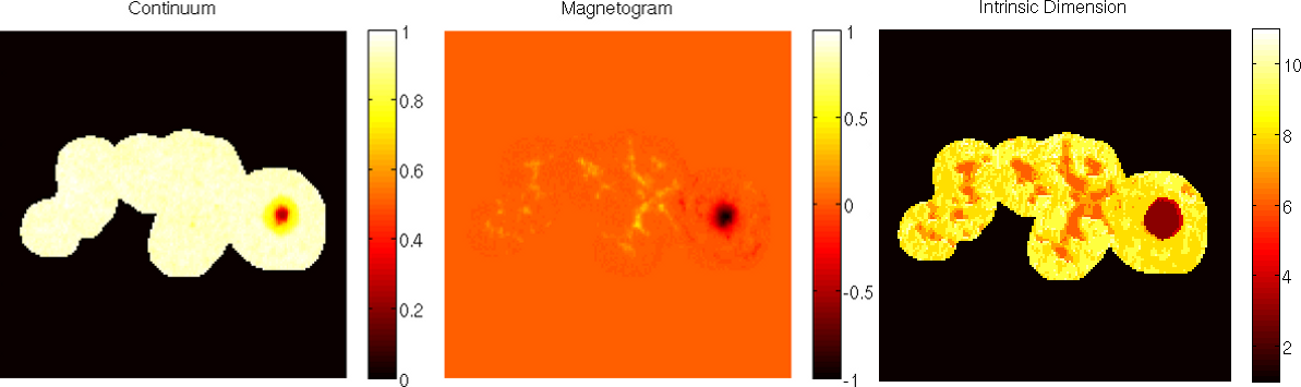
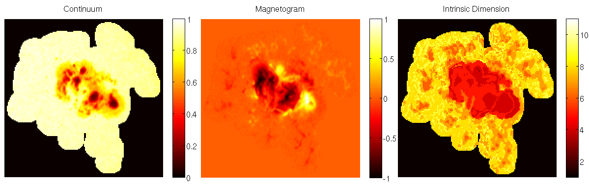
Figure 2: Examples of the estimated local intrinsic dimension using the $k$-NN method for an $\alpha$ group (top) and a $\beta\gamma\delta$ group (bottom). Regions with more spatial structure have lower intrinsic dimension.

Table 2 provides the mean and standard deviation of the intrinsic dimension estimates within the sunspots and magnetic fragments. These statistics are also provided for ARs within the main Mount Wilson classes ($\alpha$, $\beta$, $\beta\gamma$, and $\beta\gamma\delta$). We provide PCA results for the cases where we estimate the intrinsic dimension as the number of components required to explain $97\%$ and $98\%$ of the variance, respectively. For the $k$-NN method, we provide the results in two ways. For one, we take the mean of local intrinsic dimensions within each image (separating the ‘sunspot’ from the ‘magnetic fragments’) and then calculate the mean and standard deviation of these means. The statistics in this category correspond to the mean and standard deviation of the average intrinsic dimension of each image and are more directly comparable to the PCA results. However these results may be affected slightly by small sunspot groups. For the other approach, we pool all of the local estimates (again separating sunspots from magnetic fragments) and then calculate the mean and standard deviation. These results correspond to the mean and standard deviation of the pixels within each region and category and are less affected by small sunspot groups.

Table 2: Estimated intrinsic dimension results for different groups of ARs in the form of mean$\pm$standard deviation. The complex ARs have higher intrinsic dimension within the sunspots than the simple ARs but lower intrinsic dimension within the magnetic fragments.

	$\alpha$	$\beta$	$\beta\gamma$	$\beta\gamma\delta$	All
Sunspots $k$-NN, pooled	$3.9\pm 1.2$	$4.4\pm 1.0$	$4.4\pm 0.9$	$4.5\pm 0.7$	$4.3\pm 1.0$
Sunspots $k$-NN, means	$4.0\pm 1.0$	$4.8\pm 1.2$	$4.4\pm 0.6$	$4.4\pm 0.4$	$4.5\pm 1.0$
Sunspots PCA $97\%$	$3.7\pm 0.8$	$4.4\pm 0.9$	$4.3\pm 0.6$	$4.2\pm 0.5$	$4.3\pm 0.8$
Sunspots PCA $98\%$	$4.5\pm 0.9$	$5.2\pm 1.0$	$5.1\pm 0.8$	$5.0\pm 0.5$	$5.0\pm 0.9$
Fragments $k$-NN, pooled	$8.0\pm 1.1$	$8.0\pm 1.2$	$7.7\pm 1.2$	$7.6\pm 1.2$	$8.0\pm 1.2$
Fragments $k$-NN, means	$8.0\pm 0.4$	$7.9\pm 0.5$	$7.6\pm 0.5$	$7.6\pm 0.5$	$7.8\pm 0.5$
Fragments PCA $97\%$	$7.7\pm 1.6$	$7.1\pm 1.2$	$6.2\pm 1.2$	$6.2\pm 1.3$	$6.8\pm 1.4$
Fragments PCA $98\%$	$9.1\pm 1.6$	$8.5\pm 1.3$	$7.5\pm 1.2$	$7.4\pm 1.3$	$8.1\pm 1.4$

From Table 2, it is clear that the intrinsic dimension is lower within the sunspots than in the magnetic fragments for all methods. This is expected as there is more spatial structure within the images inside the sunspots than in the magnetic fragments, especially in the continuum image.

The average PCA estimate with a 97% threshold and the average mean $k$-NN estimate give similar results inside the sunspot while the average 98% PCA estimate is closest to the average mean $k$-NN estimate within the magnetic fragments. If linear methods were not sufficient to represent the spatial and modal dependencies, we would expect the PCA results to be much higher than the $k$-NN results when using comparable thresholds as more linear than nonlinear components would be required to accurately represent the data. However, this close agreement between the general and linear results suggests that linear methods are sufficient and that linear dictionary methods would be appropriate for these data.

3.4 Patterns Within the Mount Wilson Groups

For both the PCA and $k$-NN methods, the average estimated intrinsic dimension is lower within the sunspots in $\alpha$ groups than in the more complex groups such as $\beta\gamma\delta$. This is consistent with Figure 2 and may be related to the lower complexity of $\alpha$ groups. These exhibit more spatially coherent images, which can be described using a lower number of basis elements, and hence have a lower intrinsic dimension.

Within the magnetic fragments, the opposite trend occurs where the less complex groups have higher intrinsic dimension. This suggests that the magnetic fragments are fewer, weaker, and less structured outside of the $\alpha$ and $\beta$ groups compared to the more complex regions, leading to a more noise-like background in their magnetic fragments. This hypothesis is supported by the normalized histograms of the mean $k$-NN estimates of intrinsic dimension and the normalized histograms of the pooled $k$-NN estimates in Figures 3 and 4. The histograms of mean intrinsic dimension show that within the magnetic fragments, $\alpha$ groups generally have higher mean intrinsic dimension than $\beta\gamma\delta$ groups. In fact, no $\alpha$ groups have a mean intrinsic dimension less than 7.5 within the magnetic fragments. However, the normalized histograms of the individual patch estimates show a significant number of patches with intrinsic dimension less than 7.5 within the fragments. This suggests that for each $\alpha$ group, the majority of the patches have higher intrinsic dimension in the magnetic fragments and are thus more noise-like. In contrast, there are some $\beta\gamma\delta$ groups where the mean intrinsic dimension of the magnetic fragments is lower (less than 7.5) and so these magnetic fragments are dominated by patches with more structure.

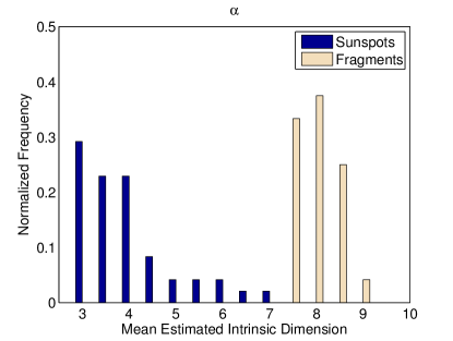
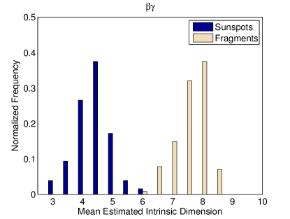
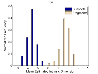
Figure 3: Normalized histograms of mean estimated intrinsic dimension of $\alpha$, $\beta,$ $\beta\gamma$, and $\beta\gamma\delta$ groups using the $k$-NN method. The distributions of intrinsic dimension differ by complexity with simpler AR groups having higher (resp. lower) intrinsic dimension within the sunspot (resp. magnetic fragments).

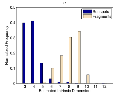
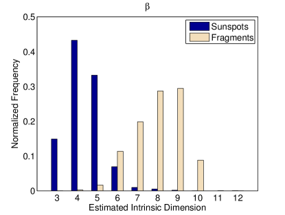
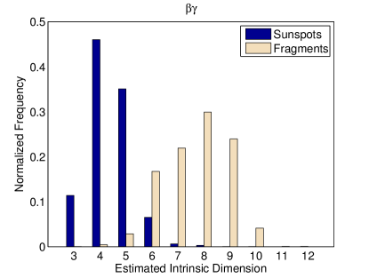
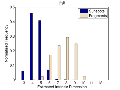
Figure 4: Normalized histograms of pooled local estimates of intrinsic dimension of $\alpha$, $\beta,$ $\beta\gamma$, and $\beta\gamma\delta$ groups using the $k$-NN method. The distributions of intrinsic dimension differ by complexity with simpler AR groups having higher (resp. lower) intrinsic dimension within the sunspot (resp. magnetic fragments).

Table 2 also shows that the standard deviation of the estimates within the sunspots decreases as the complexity increases as measured by the Mount Wilson classification scheme. The histograms in Figures 3 and 4 can be used to determine the cause. From the histograms, it is clear that within the sunspots the intrinsic dimension of $\alpha$ groups does not have a Gaussian distribution. In this case, most of the estimates are between 3 and 5. However, there are a significant number of outliers with intrinsic dimension greater than 5. The presence of these outliers contributes to the high standard deviation. This is in contrast to the intrinsic dimension of $\beta\gamma$ and $\beta\gamma\delta$ groups inside the sunspot which have fewer outliers and thus smaller standard deviations.

The outliers in the $\alpha$ groups correspond to small sunspots. The number of pixels within the $\alpha$ sunspots with average intrinsic dimension $\geq 6$ range between 10 and 53 with a median of 16. In these cases, the spatial structure of the sunspots may be more similar to the magnetic fragments than the spatial structure of larger sunspots. Thus the intrinsic dimension is higher in the small sunspots.

A similar phenomenon occurs within the $\beta$ groups. Note that in Table 2, the average and standard deviation of the mean intrinsic dimension of the $\beta$ groups within the sunspots is higher than for all other groups. This is also caused by a few outliers that have high average intrinsic dimension due to the small size of the sunspots. When individual local intrinsic dimension estimates of the patches from these small sunspots are pooled with the estimates from all other $\beta$ patches, the average intrinsic dimension is more aligned with that of the other Mount Wilson types. Additionally, ignoring the biggest outliers in the mean intrinsic dimension (defined as having mean intrinsic dimension $>6.25$) gives an average mean intrinsic dimension of 4.6 for the $\beta$ groups which is more aligned with the other groups.

The distribution of intrinsic dimension within the magnetic fragments also differs by complexity based on Figures 3 and 4. The complex ARs have more patches and images with lower intrinsic dimension than the simple sunspots which is consistent with Table 2.

In summary, based on the estimated intrinsic dimension of the image patches, relatively few parameters are required to accurately represent the data. We have found that the distribution of local intrinsic dimension varies based on the complexity of the sunspot group with the more complex sunspots having higher (resp. lower) intrinsic dimension within the sunspot (resp. magnetic fragments). Additionally, the standard deviation of the intrinsic dimension is higher within the sunspot in the simpler sunspots than the complex ARs. This is due to the presence of small sunspots among the simpler ARs that tend to have less spatial structure and thus a higher intrinsic dimension than typical sunspots. We have also shown that linear methods should be sufficient to accurately analyze the data.

4 Spatial and Modal Correlations

The results in the previous section indicate that linear methods are likely sufficient to represent the spatial and modal dependencies within a sunspot. We therefore analyze the linear correlation over patches using partial correlation and canonical correlation analysis (CCA).

The partial correlation is proportional to the inverse of the correlation matrix and analyzes the pixel-to-pixel correlation when the influence of all other pixels has been removed. It provides insight into how large a patch should be used to sufficiently capture the spatial and modal correlations in future analysis.

CCA on the other hand is determined by finding the most correlated linear combinations of pixels from each image, solved as a generalized eigenvalue problem, which is useful for determining the degree of mutual correlation between two modalities. If the two modalities are independent, there is no benefit in processing them together, while if the two modalities are strongly dependent, processing only one of the modalities is sufficient since the other modality would not contain any additional information.

4.1 Partial Correlation: Methodology

The partial correlation measures the correlation between two random variables while conditioning on the remaining random variables. The intuition behind partial correlation can be best explained with the linear regression concept. Suppose you want to compute the partial correlation between two variables $X_{1}$ and $X_{2}$ given a set of variables $\mathcal{X}$. First, compute the linear regression using variables in $\mathcal{X}$ to explain $X_{1}$ and obtain the associated residuals $r_{X_{1}}$. Proceed similarly for $X_{2}$ and get residuals $r_{X_{2}}$. The partial correlation between $X_{1}$ and $X_{2}$ is then equal to the (usual) correlation between $r_{X_{1}}$ and $r_{X_{2}}$, for which the effect of variables $\mathcal{X}$ have been removed.

In our context, let $\mathbf{x}$ be a patch from the continuum image, and $\mathbf{|y}|$ be the magnitude (entry-wise absolute value) of the corresponding patch from the magnetogram. The partial correlation matrix $\mathbf{P}=\left(\begin{array}[]{cc}\mathbf{P}_{\mathbf{xx}}&\mathbf{P}_{\mathbf{x|y|}}\\ \mathbf{P}_{\mathbf{|y|x}}&\mathbf{P}_{\mathbf{|y||y|}}\end{array}\right)$ and its off-diagonal elements can be derived from the inverse correlation matrix (see Appendix A.2). We use the magnitude of the magnetogram data since both positive and negative polarities affect the continuum image in similar ways.

4.2 Partial Correlation: Results

Figure 5 gives the estimated partial correlation matrices when using $3\times 3$ and $5\times 5$ patches. The patches are extracted from all of the active regions and divided using the STARA and SMART masks into sunspots and magnetic fragments as before. The partial correlation of $3\times 3$ patches is quite strong within both modalities. Based on a false alarm rate of $0.05$, the theoretical thresholds for significance for the partial correlation (Hero and Rajaratnam, 2011) of the $3\times 3$ patches are approximately $0.0070$ and $0.0014$ for within the sunspots and magnetic fragments, respectively. For the $5\times 5$ patches, the thresholds are $0.0080$ and $0.0016$, respectively. Given these thresholds, the partial correlation is statistically significant for nearly all values within the modalities ($\mathbf{P}_{\mathbf{xx}}$ and $\mathbf{P}_{\mathbf{|y||y|}}$) using the $3\times 3$ patches.

The cross-partial correlation when using the signed magnetic field (i.e. $\mathbf{P}_{\mathbf{xy}}$ and $\mathbf{P}_{\mathbf{yx}}$) is very near zero in both regions (not shown). However, when we take the absolute value of the magnetogram patches, then the magnitude of the cross-partial correlation ($\mathbf{P}_{\mathbf{x|y}|}$ and $\mathbf{P}_{|\mathbf{y|x}}$) is much higher in both regions suggesting that the correlation between the modalities is significant. The partial correlation is also stronger in magnitude in all cases within the sunspots than within the magnetic fragments.

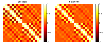
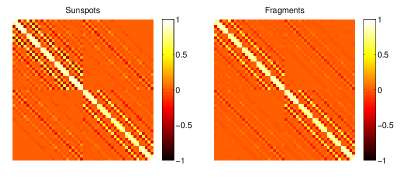
Figure 5: Estimated partial correlation matrices of patch data from within the sunspots and the magnetic fragments using $3\times 3$ (left) and $5\times 5$ (right) patches. The theoretical thresholds (Hero and Rajaratnam, 2011) for significance to attain a $0.05$ false alarm rate are $0.0070$ and $0.0014$ for within the sunspots and magnetic fragments, respectively when using a $3\times 3$ patch. For the $5\times 5$ patch, the thresholds are $0.0080$ and $0.0016$, respectively. Statistically insignificant values are set to zero.

The partial correlation matrices are very structured. In both sunspots and magnetic fragments, the pentadiagonal-like structure within the modalities suggests that the image is generally stationary with approximately a third order nearest neighbor Markov structure in the pixels. Such structure is clearly seen in the matrices for $5\times 5$ patches. The cross-partial correlation also has a pentadiagonal-like structure although the correlation is not as strong as within the modalities.

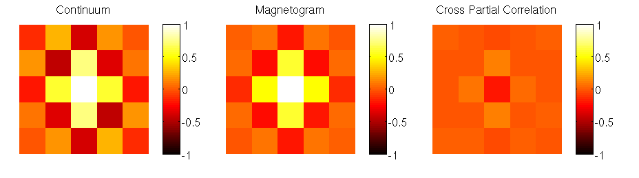
Figure 6: Partial correlation patches extracted from the columns in the sunspot partial correlation matrix corresponding to the center pixels. The partial correlation is stronger within the continuum.

To better see the spatial correlations, in Figure 6 we plot the partial correlation patches taken from the columns of the sunspot partial correlation matrix corresponding to the center pixels when using $5\times 5$ patches. Figure 6 shows clearly the greater partial correlation within the continuum. It also highlights that correlation is slightly higher in magnitude in the vertical direction than the horizontal direction. Nearly all sunspots in this study are located within $(-30^{\circ},+30^{\circ})$ from both the central meridian and the equator, and so projection effect are unlikely to cause this difference. The difference in correlation may be a feature of the sunspots themselves, but this may be difficult to determine since the difference in partial correlation is small.

Some slight differences exist in the partial correlation matrices restricted to certain Mount Wilson classes. As an example, Figure 7 contains the partial correlation matrices within the sunspots after restricting the data to $\alpha$ and $\beta$ groups as well as the difference between the absolute value of the two matrices. The $\alpha$ partial correlation matrix is higher in magnitude within the modalities than the $\beta$ matrix but lower between the modalities. Within modalities, the strongest differences (a maximum of 0.056 and 0.067 within the continuum and magnetogram, respectively) are in the entries that correspond to pixels that are farther away from each other. In contrast, within the cross-partial correlation, the strongest differences (a maximum of 0.072) between the two AR types are in the entries that correspond to pixels that are close to each other. A similar pattern holds when comparing the $\alpha$ matrix to the matrices of the more complex groups.

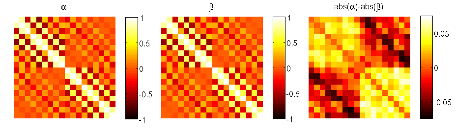
Figure 7: Partial correlation matrices within the sunspots using the data from $\alpha$ (left) and $\beta$ ARs (center). Statistically insignificant values are again set to zero. (Right) difference between the absolute value of the $\alpha$ and $\beta$ matrices. The $\alpha$ sunspots are more (resp. less) strongly correlated within (resp. between) the modalities than the $\beta$ groups.

Overall, the partial correlation matrices indicate that no larger than a $5\times 5$ patch is necessary to capture the local spatial dependencies. A $5\times 5$ patch of pixels corresponds roughly to the size of a mesogranule (Rast, 2003; Rieutord et al., 2000). This suggests that within the magnetic fragments, it is likely that the granules and mesogranules within the photosphere contribute to the local spatial dependencies. Within the sunspots, a $5\times 5$ patch corresponds to the size of the characteristic length of the largest penumbral filaments (Tiwari et al., 2013) which suggests that on average the local spatial dependencies are minimal beyond this scale. This analysis, however, does not rule out long-range spatial dependencies, which are more difficult to assess due to the large dimensionality. Future work will focus on this.

In the remainder of our analysis, we choose a $3\times 3$ patch for the reasons mentioned in Section 2: to ensure that we capture the features of small sunspots and to limit the effects high dimension on the accuracy of the analysis. Given these concerns, we see that $3\times 3$ patches capture most of the spatial correlation. This is evident from Figure 5 where the partial correlation between pixels on opposite corners of a $3\times 3$ patch is near zero and other pixels that are similarly far away from each other have low partial correlation. Thus a $3\times 3$ patch strikes a good balance between scale, extrinsic dimension, and capturing the spatial correlation.

4.3 Canonical Correlation Analysis: Methodology

To further investigate the correlation between the modalities, we use canonical correlation analysis (CCA) on the continuum patch $\mathbf{x}$ and the magnitude of the magnetogram patch $\mathbf{y}$. CCA finds patterns and correlations between two multivariate data sets (Muller, 1982; Nimon et al., 2010) and was used previously in the context of space weather e.g. for the combined analysis of solar wind and geomagnetic index data sets (Borovsky, 2014).

In our application, CCA provides linear combinations of continuum patches $\mathbf{x}$ that are most correlated with linear combinations of magnetogram patches $\mathbf{y}$. In other words, all correlations between the continuum and magnetogram patches are channeled through the canonical variables. Formally, CCA finds vectors $\mathbf{a}_{i}$ and $\mathbf{b}_{i}$ for $i=1,\dots,m^{2}$ such that the correlation $\rho_{i}=\text{corr}(\mathbf{a}_{i}^{T}\mathbf{x},\mathbf{b}_{i}^{T}|\mathbf{y}|)$ is maximized and the pair of random variables $u_{i}=\mathbf{a}_{i}^{T}\mathbf{x}$ and $v_{i}=\mathbf{b}_{i}^{T}|\mathbf{y}|$ are uncorrelated with all other pairs $u_{j}$ and $v_{j}$, $j\neq i$. The variables $u_{i}$ and $v_{i}$ are called the $i$th pair of canonical variables while the vectors $\mathbf{a}_{i}$ and $\mathbf{b}_{i}$ are the canonical vectors. The solution $\mathbf{a}_{i}$ is the $i$th eigenvector of the matrix $\Sigma_{\mathbf{xx}}^{-1}\Sigma_{\mathbf{x|y}|}\Sigma_{|\mathbf{y||y|}}^{-1}\Sigma_{|\mathbf{y|x}}$ which are taken from the covariance matrix. The vector $\mathbf{b}_{i}$ is found similarly (Härdle and Simar, 2007).

4.4 Canonical Correlation Analysis: Results

Here we focus on $3\times 3$ patches and apply CCA to all 424 image pairs using the magnitude of the magnetogram patches. Figure 8 (left and center) shows histograms of the estimated values of $\rho_{1}$. Within the sunspots, there are many groups with a near perfect correlation between the modalities and none of the groups have an estimated value below $0.41$. The right plot in Figure 8 plots the estimated values of $\rho_{1}$ vs. the number of samples used within the sunspots. Based on this plot, there are many ARs with high correlation and few patch samples suggesting that the correlation may be spurious. However, all of the estimated values are statistically significant as defined by the threshold given by Hero and Rajaratnam (2011) using a false alarm rate of 0.05 (shown as the magenta line in Figure 8).

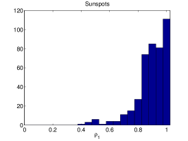
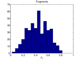
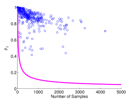
Figure 8: Histograms of estimated $\rho_{1}$ using CCA for within the sunspots (left) and the magnetic fragments (center) using $3\times 3$ patches. Right: Scatter plot of $\rho_{1}$ values and the number of samples available for within the sunspots. All points are above the magenta line which gives the threshold for statistical significance at a false alarm rate of 0.05 (Hero and Rajaratnam, 2011).

The histogram of $\rho_{1}$ within the magnetic fragments (Fig. 8, center) is quite different from the sunspot histogram (Fig. 8, left). $\rho_{1}$ is generally lower within the magnetic fragments than within the sunspots which is consistent with the results in Figure 5. All of the $\rho_{1}$ values are statistically significant.

The distributions of $\rho_{1}$ differ slightly when comparing simple sunspot groups ($\alpha$ and $\beta$) with complex groups ($\beta\gamma$ and $\beta\gamma\delta$). Figure 9 shows that complex groups generally have lower correlation between the modalities within the sunspots than the simpler groups. The estimated Hellinger distance (see Appendix A.3) between the distributions using the divergence estimator in Moon and Hero III (2014a, b) is 0.22. Based on the central limit theorem of the estimator (Moon and Hero III, 2014b), this value is statistically significant with a $p$-value of $1.6\times 10^{-12}$. At least some of this difference is likely due to the smaller size of the simpler groups (and thus smaller sample size). However, it is unlikely to fully explain the difference given that there are many simple sunspot groups with high correlation and sufficient sample size.

Within the magnetic fragments, there are many more simple regions than complex regions with $\rho_{1}<0.4$ (see the histogram in Figure 9, right). This could be related to the same phenomena that causes the intrinsic dimension to be higher within the magnetic fragments of simple sunspot groups observed in Section 3.3. However, the estimated Hellinger distance between these distributions is 0.016. Using the same statistical test, this estimate is not statistically significant with a $p$-value of $0.31$. Thus the distributions are not statistically different from each other.

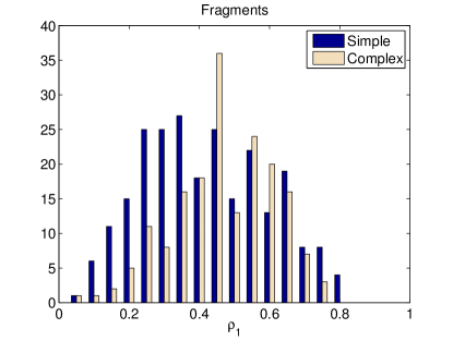
Figure 9: $\rho_{1}$ histograms of complex ($\beta\gamma$ and $\beta\gamma\delta$) and simple ($\alpha$ and $\beta$) regions within the sunspots (left) and the magnetic fragments (right). The simple ARs are generally more correlated within the sunspots but less correlated within the magnetic fragments. The difference between the sunspot distributions, as measured by the Hellinger distance, is statistically significant.

To analyze the spatial patterns that produce the highest correlation between modalities, we apply CCA to the entire data set. Figure 10 plots $\rho_{i}$ for $i=1,\dots,9$ for within the sunspots and within the magnetic fragments. The $\rho_{i}$ are all statistically significant. Notice that the $\rho_{i}$ are higher within the sunspots than the magnetic fragments which is consistent with the results in Figures 5 and 8.

Figure 10 shows the canonical patches $\mathbf{a}_{i}$ and $\mathbf{b}_{i}$ for $i=1,\dots,6$ when using all the data from within the sunspots. These are the spatial patterns within the two modalities that are most correlated with each other. The canonical patches have a “saddle-like” appearance where the gradient is positive in some directions and negative in others. For example, in $\mathbf{a}_{4}$, the pixels to the left and right of the center are very negative but the pixels in the corners are all very positive. Note that these vectors correspond to centered values with respect to the mean patches.

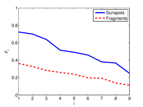
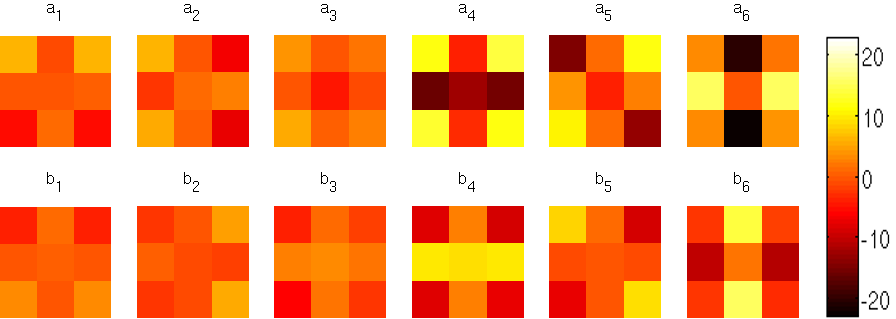
Figure 10: (Left) Plot of the estimated $\rho_{i}$ using CCA on the entire data set for $i=1,\dots,9$. All values are statistically significant (Hero and Rajaratnam, 2011). (Right) Canonical patches $\mathbf{a}_{i}$ (top) and $\mathbf{b}_{i}$ (bottom) for $i=1,\dots,6$ when using the entire data set from within the sunspots. The $\mathbf{b}_{i}$s are approximately equal to the negative of the $\mathbf{a}_{i}$s.

Comparing the $\mathbf{a}_{i}$s to the $\mathbf{b}_{i}$s shows that the $\mathbf{b}_{i}$s are approximately equal to the negative of the $\mathbf{a}_{i}$s. This makes sense as sunspots within the continuum images correspond to a decrease in value relative to the background while ARs within the magnitude of the magnetogram images correspond to an increase in value relative to the background.

We also performed CCA separately on the data from the Mount Wilson classes. Figure 11 plots the $\rho_{i}$ values for each class and the first canonical patches $\mathbf{a}_{1}$ and $\mathbf{b}_{1}$. For $\rho_{1}$ and $\rho_{2}$, the values for each class decrease in order of complexity ($\alpha,$ $\beta$, $\beta\gamma,$ $\beta\gamma\delta$). This is consistent with our comparison of the partial correlation matrices in Figure 7 where the partial correlation was generally higher (in magnitude) for the $\alpha$ groups than the others. This is also consistent with the intrinsic dimension analysis in Section 3 where the intrinsic dimension generally increases with complexity. This is because if the correlation between and within modalities is higher, then fewer parameters are required to accurately describe the data which results in a lower intrinsic dimension.

The canonical patches $\mathbf{a}_{1}$ and $\mathbf{b}_{1}$ have similar patterns across the different classes although the patches for the $\beta\gamma$ class are flipped compared to the others. The magnitude of the values in the $\beta\gamma\delta$ patches are also smaller than the those of the other patches.

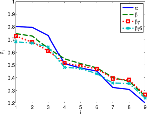
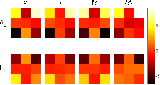
Figure 11: (Left) Plot of the estimated $\rho_{i}$ using CCA on data segregated by Mount Wilson classes for $i=1,\dots,9$ within the sunspots $\alpha$ groups start out with the highest correlation. (Right) Canonical patches $\mathbf{a}_{1}$ (top) and $\mathbf{b}_{1}$ (bottom) for the Mount Wilson classes within the sunspots. Again, the $\mathbf{b}_{1}$s are approximately equal to the negative of the $\mathbf{a}_{1}$s as in Figure 10 but the patches differ slightly from class to class.

Overall, the results of this section suggest that the two modalities are correlated in both the sunspots and the magnetic fragments and are therefore not independent. The correlation is stronger within the sunspots compared to the magnetic fragments and stronger within the sunspots in simple ARs compared to complex ARs. However, the correlation is not perfect and so there may be an advantage to including both modalities in the classification of sunspots and flare prediction.

5 Conclusion

Existing AR categorical classification systems such as the Mount Wilson and McIntosh schemes describe geometrical arrangements of the magnetic field at the largest length scale. In this work, we have focused on the properties of the ARs at fine length scale. We showed that when we analyze the global statistics or attributes of these local properties, we find differences between the simple and complex ARs as defined using the large scale characteristics. So by this approach, we are analyzing both the large and fine scale properties of the images. Such results might be due to the multi-scale properties of the magnetic fields, as evidenced previously in Ireland et al. (2008).

The local intrinsic dimension based on the $k$-NN approach combines both continuum and magnetogram observations and provides some measure of local regularity for those images. Further differences between the Mount Wilson classes may be found by comparing the histograms or distributions of local intrinsic dimension of each individual AR instead of only comparing the means or pooled estimates as we did in this paper. There are several options to perform such comparisons. Each histogram could be treated as a vector, or we could consider the underlying probability density function within the framework of functional analysis. Supervised (using Mount Wilson classes) or unsupervised classification could be performed. Another option would be to view the set of histograms belonging to a specific class as samples from a distribution of vectors (or a distribution of probability density functions). Different classes could then be compared using divergence measures such as the Hellinger distance described in Appendix A.3.

This work also highlighted specific behaviors of the core of active regions (that corresponds to the sunspot masks in continuum) and magnetic fragments (the surrounding part of AR), as well as the difference of these two regions as a function of the Mount Wilson classification. We found that within the sunspots, the spatial and modal correlations are stronger than within the magnetic fragments. Additionally, simpler ARs were found to have higher correlation between the modalities within the sunspots than the complex ARs.

This study paves the way for further analysis based on dictionary learning. Knowledge of the intrinsic dimension allows us to choose the dictionary size. Moreover the results of Section 3 showed that linear dictionary learning methods are sufficient. The spatial and modal correlation analysis in Section 4 justifies a choice of a patch size of $3\times 3$ and confirms that both modalities (continuum and magnetogram) should be used in dictionary learning.

Appendix A Method Details

A.1 Intrinsic Dimension Estimation of Manifolds

Consider data that are described in an extrinsic Euclidean space of $d$ dimensions. However, suppose the data actually lie on a lower dimensional manifold $\mathcal{M}$. Thus the intrinsic dimension $m$ of the data corresponds to the dimension of $\mathcal{M}$. For example, data may be given to us in a 3 dimensional space but lie on the surface of a sphere. Thus the intrinsic dimension of the data would be 2.

In some cases, data points from the same data set may lie on different manifolds. For example, part of the data with an extrinsic dimension of 3 could lie on the surface of a sphere ($m=2$) while another part may lie on a circle ($m=1$). We then say that data points from these different manifolds have a different local intrinsic dimension. The local intrinsic dimension gives some measure of the local complexity of the image. Additionally, the local intrinsic dimension is useful for dictionary learning because we can use it to determine whether different-sized dictionaries should be used for different regions, e.g. within the sunspots and outside of the sunspots.

We now describe the $k$-NN estimator of intrinsic dimension in more detail. For a set of independently identically distributed random vectors $\mathbf{Z}_{n}=\{\mathbf{z}_{1},\dots,\mathbf{z}_{n}\}$ with values in a compact subset of $\mathbb{R}^{d}$, the $k$-nearest neighbors of $\mathbf{z}_{i}$ in $\mathbf{Z}_{n}$ are the $k$ points in $\mathbf{Z}_{n}\backslash\{\mathbf{z}_{i}\}$ closest to $\mathbf{z}_{i}$ as measured by the Euclidean distance $||\cdot||$. The $k$-NN graph is then formed by assigning edges between a point in $\mathbf{Z}_{n}$ and its $k$-nearest neighbors. The intrinsic dimension is related to the total edge length of the $k$-NN graph and can be estimated based on this relationship. The $k$-NN graph is then formed by assigning edges between a point in $\mathbf{Z}_{n}$ and its $k$-nearest neighbors and has total edge length defined as

$$L_{\gamma,k}(\mathbf{Z}_{n})=\sum_{i=1}^{n}\sum_{\mathbf{z}\in\mathcal{N}_{k,i}}||\mathbf{z}-\mathbf{z}_{i}||^{\gamma},$$

where $\gamma>0$ is a power weighting constant and $\mathcal{N}_{k,i}$ is the set of $k$ nearest neighbors of $\mathbf{z}_{i}.$ It has been shown that for large $n$,

$$L_{\gamma,k}(\mathbf{Z}_{n})=n^{\alpha(m)}c+\epsilon_{n},$$

where $\alpha=(m-\gamma)/m$, $c$ is a constant with respect to $\alpha(m)$, and $\epsilon_{n}$ is an error term that decreases to zero a.s. as $n\rightarrow\infty$ (Costa and Hero III, 2006). A global intrinsic dimension estimate $\hat{m}$ is found based on this relationship using non-linear least squares over different values of $n$ (Carter et al., 2010).

A local estimate of intrinsic dimension at a point $\mathbf{z}_{i}$ can be found by running the algorithm over a smaller neighborhood about $\mathbf{z}_{i}.$ The variance of this local estimate is then reduced by smoothing via majority voting in a neighborhood of $\mathbf{z}_{i}$ (Carter et al., 2010).

A.2 Partial Correlation

Let $\mathbf{z}$ be a random vector with size $m$. Let $\Sigma$ be the covariance matrix of $\mathbf{z}$, that is $\Sigma_{ij}=\text{Cov}(z_{i},z_{j})$, and let $\mathbf{K}=\Sigma^{-1}$ be the inverse of the covariance matrix, also called the precision matrix.

The partial correlation between $z_{i}$ and $z_{j}$ given all the other variables $\mathbf{z}\backslash\{z_{i},z_{j}\}$ measure the degree of correlation between these two variables after removing the effect of the remaining ones. Let $\mathbf{P}_{ij}$ denote the partial correlation between $z_{i}$ and $z_{j}$. It has been shown (Lauritzen, 1996) that $\mathbf{P}_{ij}$ can be related to the elements of the precision matrix $\mathbf{K}$ as follows:

$$\begin{array}[]{cc}\mathbf{P}_{ij}=-\frac{K_{ij}}{\sqrt{K_{ii}K_{jj}}},&i\neq j.\end{array}$$

A.3 Estimating the Hellinger Distance

Information divergences are a class of functionals that measure the difference between two probability distributions. The most popular divergence measure is the Kullback-Leibler divergence (Kullback and Leibler, 1951). The Hellinger distance is another divergence measure and is defined as

$$H(f,g)=\sqrt{1-\int\sqrt{f(x)g(x)}dx},$$

where $f$ and $g$ are the two probability densities being compared. The Hellinger distance is a metric which is not true of divergences in general. we use the nonparametric divergence estimator derived in Moon and Hero III (2014a, b). In Moon and Hero III (2014a), it was shown that this estimator converges to the true divergence with mean squared error convergence rate $O(1/T)$ where $T$ is the number of samples from each probability distribution. In Moon and Hero III (2014b), it was shown that the distribution of the normalized version of this estimator converges to the standard normal distribution. We can use this fact combined with a bootstrap estimate (Efron and Tibshirani, 1994) of the variance of the estimator to test the hypothesis that the divergence is zero (and hence the distributions are equal).

References

- Abramenko (2005) Abramenko, V. I. Multifractal Analysis Of Solar Magnetograms. Solar Physics, 228, 29–42, 2005. 10.1007/s11207-005-3525-9.
- Bloomfield et al. (2012) Bloomfield, D. S., P. A. Higgins, R. T. J. McAteer, and P. T. Gallagher. Toward Reliable Benchmarking of Solar Flare Forecasting Methods. Astrophysical Journal, Letters, 747, L41, 2012. 10.1088/2041-8205/747/2/L41.
- Bornmann and Shaw (1994) Bornmann, P. L., and D. Shaw. Flare rates and the McIntosh active-region classifications. Solar Physics, 150, 127–146, 1994. 10.1007/BF00712882.
- Borovsky (2014) Borovsky, J. E. Canonical correlation analysis of the combined solar wind and geomagnetic index data sets. Journal of Geophysical Research (Space Physics), 119, 5364–5381, 2014. 10.1002/2013JA019607.
- Bühlmann and Van De Geer (2011) Bühlmann, P., and S. Van De Geer. Statistics for high-dimensional data: methods, theory and applications. Springer Science & Business Media, 2011.
- Cadavid et al. (2008) Cadavid, A. C., J. K. Lawrence, and A. Ruzmaikin. Principal Components and Independent Component Analysis of Solar and Space Data. Solar Physics, 248, 247–261, 2008. 10.1007/s11207-007-9026-2.
- Carter et al. (2010) Carter, K. M., R. Raich, and A. O. Hero. On local intrinsic dimension estimation and its applications. Signal Processing, IEEE Transactions on, 58(2), 650–663, 2010.
- Colak and Qahwaji (2008) Colak, T., and R. Qahwaji. Automated McIntosh-Based Classification of Sunspot Groups Using MDI Images. Solar Physics, 248, 277–296, 2008. 10.1007/s11207-007-9094-3.
- Colak and Qahwaji (2009) Colak, T., and R. Qahwaji. Automated Solar Activity Prediction: A hybrid computer platform using machine learning and solar imaging for automated prediction of solar flares. Space Weather, 7, S06001, 2009. 10.1029/2008SW000401.
- Conlon et al. (2008) Conlon, P. A., P. T. Gallagher, R. T. J. McAteer, J. Ireland, C. A. Young, P. Kestener, R. J. Hewett, and K. Maguire. Multifractal Properties of Evolving Active Regions. Solar Physics, 248, 297–309, 2008. 10.1007/s11207-007-9074-7.
- Conlon et al. (2010) Conlon, P. A., R. T. J. McAteer, P. T. Gallagher, and L. Fennell. Quantifying the Evolving Magnetic Structure of Active Regions. Astrophysical Journal, 722, 577–585, 2010. 10.1088/0004-637X/722/1/577.
- Costa and Hero III (2006) Costa, J. A., and A. O. Hero III. Determining intrinsic dimension and entropy of high-dimensional shape spaces. In Statistics and Analysis of Shapes, 231–252. Springer, 2006.
- Dobigeon et al. (2014) Dobigeon, N., J.-Y. Tourneret, C. Richard, J. Bermudez, S. Mclaughlin, and A. O. Hero. Nonlinear unmixing of hyperspectral images: Models and algorithms. Signal Processing Magazine, IEEE, 31(1), 82–94, 2014.
- Dudok de Wit et al. (2013) Dudok de Wit, T., S. Moussaoui, C. Guennou, F. Auchère, G. Cessateur, M. Kretzschmar, L. A. Vieira, and F. F. Goryaev. Coronal Temperature Maps from Solar EUV Images: A Blind Source Separation Approach. Solar Physics, 283, 31–47, 2013. 10.1007/s11207-012-0142-2.
- Dudok DeWit and Auchère (2007) Dudok DeWit, T., and F. Auchère. Multispectral analysis of solar EUV images: linking temperature to morphology. Astronomy and Astrophysics, 466, 347–355, 2007. 10.1051/0004-6361:20066764.
- Efron and Tibshirani (1994) Efron, B., and R. Tibshirani. An Introduction to the Bootstrap. Chapman and Hall, 1994.
- Elad and Aharon (2006) Elad, M., and M. Aharon. Image Denoising Via Sparse and Redundant Representations Over Learned Dictionaries. Image Processing, IEEE Transactions on, 15(12), 3736–3745, 2006. 10.1109/TIP.2006.881969.
- Gallagher et al. (2002) Gallagher, P. T., Y.-J. Moon, and H. Wang. Active-Region Monitoring and Flare Forecasting I. Data Processing and First Results. Solar Physics, 209, 171–183, 2002. 10.1023/A:1020950221179.
- Georgoulis (2005) Georgoulis, M. K. Turbulence In The Solar Atmosphere: Manifestations And Diagnostics Via Solar Image Processing. Solar Physics, 228, 5–27, 2005. 10.1007/s11207-005-2513-4.
- Hale et al. (1919) Hale, G. E., F. Ellerman, S. B. Nicholson, and A. H. Joy. The Magnetic Polarity of Sun-Spots. Astrophysical Journal, 49, 153, 1919. 10.1086/142452.
- Härdle and Simar (2007) Härdle, W., and L. Simar. Applied multivariate statistical analysis. Springer, 2007.
- Hero and Rajaratnam (2011) Hero, A., and B. Rajaratnam. Large-scale correlation screening. Journal of the American Statistical Association, 106(496), 1540–1552, 2011.
- Hewett et al. (2008) Hewett, R. J., P. T. Gallagher, R. T. J. McAteer, C. A. Young, J. Ireland, P. A. Conlon, and K. Maguire. Multiscale Analysis of Active Region Evolution. Solar Physics, 248, 311–322, 2008. 10.1007/s11207-007-9028-0.
- Higgins et al. (2011) Higgins, P. A., P. T. Gallagher, R. McAteer, and D. S. Bloomfield. Solar magnetic feature detection and tracking for space weather monitoring. Advances in Space Research, 47(12), 2105–2117, 2011.
- Holappa et al. (2014) Holappa, L., K. Mursula, T. Asikainen, and I. G. Richardson. Annual fractions of high-speed streams from principal component analysis of local geomagnetic activity. Journal of Geophysical Research (Space Physics), 119, 4544–4555, 2014. 10.1002/2014JA019958.
- Ireland et al. (2008) Ireland, J., C. A. Young, R. T. J. McAteer, C. Whelan, R. J. Hewett, and P. T. Gallagher. Multiresolution Analysis of Active Region Magnetic Structure and its Correlation with the Mount Wilson Classification and Flaring Activity. Solar Physics, 252, 121–137, 2008. 10.1007/s11207-008-9233-5.
- Jolliffe (2002) Jolliffe, I. T. Principal Component Analysis, 2nd edition. Springer-Verlag New York, Inc., New York, 2002.
- Kestener et al. (2010) Kestener, P., P. A. Conlon, A. Khalil, L. Fennell, R. T. J. McAteer, P. T. Gallagher, and A. Arneodo. Characterizing Complexity in Solar Magnetogram Data Using a Wavelet-based Segmentation Method. Astrophysical Journal, 717, 995–1005, 2010. 10.1088/0004-637X/717/2/995.
- Kullback and Leibler (1951) Kullback, S., and R. A. Leibler. On information and sufficiency. The Annals of Mathematical Statistics, 79–86, 1951.
- Lauritzen (1996) Lauritzen, S. Graphical Models. Clarendon Press, 1996. ISBN 9780191591228.
- Lawrence et al. (2004) Lawrence, J. K., A. Cadavid, and A. Ruzmaikin. Principal Component Analysis of the Solar Magnetic Field I: The Axisymmetric Field at the Photosphere. Solar Physics, 225, 1–19, 2004. 10.1007/s11207-004-3257-2.
- Levina and Bickel (2004) Levina, E., and P. J. Bickel. Maximum likelihood estimation of intrinsic dimension. In Advances in Neural Information Processing Systems, vol. 17, 777–784, 2004.
- Mallat and Zhang (1993) Mallat, S., and Z. Zhang. Matching pursuits with time-frequency dictionaries. Signal Processing, IEEE Transactions on, 41(12), 3397–3415, 1993. 10.1109/78.258082.
- Mayfield and Lawrence (1985) Mayfield, E. B., and J. K. Lawrence. The correlation of solar flare production with magnetic energy in active regions. Solar Physics, 96, 293–305, 1985. 10.1007/BF00149685.
- McAteer et al. (2010) McAteer, R. T. J., P. T. Gallagher, and P. A. Conlon. Turbulence, complexity, and solar flares. Advances in Space Research, 45, 1067–1074, 2010. 10.1016/j.asr.2009.08.026.
- McAteer et al. (2005) McAteer, R. T. J., P. T. Gallagher, and J. Ireland. Statistics of Active Region Complexity: A Large-Scale Fractal Dimension Survey. Astrophysical Journal, 631, 628–635, 2005. 10.1086/432412.
- McIntosh (1990) McIntosh, P. S. The classification of sunspot groups. Solar Physics, 125, 251–267, 1990. 10.1007/BF00158405.
- Moon et al. (2015) Moon, K. R., V. Delouille, J. J. Li, R. De Visscher, F. Watson, and A. O. Hero III. Image patch analysis of sunspots and active regions. II. Clustering via matrix factorization. Journal of Space Weather and Space Climate, 2015.
- Moon and Hero III (2014a) Moon, K. R., and A. O. Hero III. Ensemble estimation of multivariate f-divergence. In Information Theory (ISIT), 2014 IEEE International Symposium on, 356–360. IEEE, 2014a.
- Moon and Hero III (2014b) Moon, K. R., and A. O. Hero III. Multivariate f-Divergence Estimation With Confidence. In Advances in Neural Information Processing Systems, vol. 27, 2420–2428, 2014b.
- Moon et al. (2014) Moon, K. R., J. J. Li, V. Delouille, F. Watson, and A. O. Hero III. Image patch analysis and clustering of sunspots: A dimensionality reduction approach. In IEEE International Conference on Image Processing (ICIP), 1623–1627. IEEE, 2014.
- Muller (1982) Muller, K. E. Understanding canonical correlation through the general linear model and principal components. American Statistics, 36, 342–354, 1982.
- Nimon et al. (2010) Nimon, K., R. Henson, and M. Gates. Revisiting interpretation of canonical correlation analysis: A tutorial and demonstration of canonical commonality analysis. Multivar. Behav., 45, 702?724, 2010.
- Phillips (1991) Phillips, K. J. H. Solar flares - A review. Vistas in Astronomy, 34, 353–365, 1991. 10.1016/0083-6656(91)90014-J.
- Rast (2003) Rast, M. P. The scales of granulation, mesogranulation, and supergranulation. The Astrophysical Journal, 597(2), 1200, 2003.
- Rieutord et al. (2000) Rieutord, M., T. Roudier, J. Malherbe, and F. Rincon. On mesogranulation, network formation and supergranulation. Astronomy and Astrophysics, 357, 1063–1072, 2000.
- Sammis et al. (2000) Sammis, I., F. Tang, and H. Zirin. The Dependence of Large Flare Occurrence on the Magnetic Structure of Sunspots. Astrophysical Journal, 540, 583–587, 2000. 10.1086/309303.
- Scherrer et al. (1995) Scherrer, P. H., R. S. Bogart, R. I. Bush, J. T. Hoeksema, A. G. Kosovichev, et al. The Solar Oscillations Investigation - Michelson Doppler Imager. Solar Physics, 162, 129–188, 1995. 10.1007/BF00733429.
- Stenning et al. (2013) Stenning, D. C., T. C. M. Lee, D. A. van Dyk, V. Kashyap, J. Sandell, and C. A. Young. Morphological feature extraction for statistical learning with applications to solar image data. Statistical Analysis and Data Mining, 6(4), 329–345, 2013. 10.1002/sam.11200.
- Tiwari et al. (2013) Tiwari, S. K., M. van Noort, A. Lagg, and S. K. Solanki. Structure of sunspot penumbral filaments: a remarkable uniformity of properties. Astronomy & Astrophysics, 557, A25, 2013.
- Watson et al. (2011) Watson, F. T., L. Fletcher, and S. Marshall. Evolution of sunspot properties during solar cycle 23. Astronomy & Astrophysics, 533, A14, 2011. 10.1051/0004-6361/201116655.
- Zharkova et al. (2012) Zharkova, V. V., S. J. Shepherd, and S. I. Zharkov. Principal component analysis of background and sunspot magnetic field variations during solar cycles 21-23. Monthly Notices of the RAS, 424, 2943–2953, 2012. 10.1111/j.1365-2966.2012.21436.x.