Phantom behavior via cosmological creation of particles

Abstract

Recent determinations of the equation of state of dark energy hint that this may well be of the phantom type, i.e., $w_{de}<-1$. If confirmed by future experiments, this would strongly point to the existence of fields that violate the dominant energy condition, which are known to present serious theoretical difficulties. This paper presents an alternative to this possibility, namely, that the measured equation of state, $w_{de}$, is in reality an effective one, the equation of state of the quantum vacuum, $w_{\Lambda}=-1$, plus the negative equation of state, $w_{c}$, associated to the production of particles by the gravitational field acting on the vacuum. To illustrate this, three phenomenological models are proposed and constrained with recent observational data.

I Introduction

Recently, the analysis of a well of data provided by the Planck satellite ade strengthened still further our confidence in the, so-called, Lambda cold dark matter ($\Lambda$CDM) model. Thus far, it constitutes the most promising cosmological model in the market because, notwithstanding its simplicity, it fits rather well most observational data. By assuming a spatially flat, homogeneous, and isotropic universe, of which the main sources of gravity at present are pressureless matter (baryonic plus dark) and the energy of the quantum vacuum (the vacuum pressure is related to the latter by $p_{\Lambda}=-\rho_{\Lambda}$), it successfully describes, with just six free parameters, the evolution of our Universe up to the present era of accelerated expansion.

A crucial quantity in models based on Einstein gravity aimed at accounting for the current accelerated phase of expansion is the equation of state (EoS) of dark energy (DE), the ratio $w_{de}=p_{de}/\rho_{de}$ of the pressure to the density of dark energy. The latter drives the acceleration thanks to its highly negative pressure, $p_{de}<-\rho_{de}/3$. In the case of the $\Lambda$CDM model, this agent is nothing but the energy of the vacuum whence the corresponding EoS parameter is just $w_{\Lambda}=-1$. In spite of the success of this model, recent model-independent measurements of $w_{de}$ seem to favor a slightly more negative EoS (see, e.g., Refs. Rest , Xia , Cheng , and Shafer ), which, if confirmed, would invalidate the model. In particular, the Planck mission yields $w_{de}=-1.13^{+0.13}_{-0.10}$ ade .

Rest et al., using supernovae type Ia (SN Ia) data from the Pan-STARRS1 Medium Deep Survey in the redshift interval $0.03<z<0.65$ found $w_{de}=-1.166_{-0.069}^{+0.072}$, i.e., $w_{de}<-1$ at $2.3\sigma$ confidence level Rest . However, they caution that it is unclear whether the tension with the $\Lambda$CDM value arises from new physics or a conjunction of chance and hidden systematics. Similarly, Cheng et al. obtained $\,w_{de}=-1.16\pm 0.06$ ($w_{de}<-1$ at $2.6\sigma$) Cheng . Likewise, the authors of Ref. Shafer , using geometrical data from SN Ia, baryon acoustic oscillations (BAOs), and the cosmic microwave background (CMB) radiation, determined $w_{de}<-1$ at $\sim 1.9\sigma$ level. They conclude that, at $2\sigma$, either the Supernova Legacy Survey Conley and Panoramic Telescope and Rapid Response System data Scolnic contain unknown systematics or the Hubble constant is lower than $71$ km/s/Mpc, or else, $w_{de}<w_{\Lambda}$.

The simplest way to achieve $w_{de}<-1$ in a manner consistent with general relativity is to assume that the dark energy corresponds to some or other scalar field, called a “phantom field,” that violates the dominant energy condition by allowing its kinetic term to have the “wrong” sign Caldwell . Thus, its energy density and pressure are given by $\rho_{ph}=-\textstyle{1\over{2}}\,\dot{\phi}^{2}+V(\phi)$ and $p_{ph}=-\textstyle{1\over{2}}\,\dot{\phi}^{2}-V^{2}(\phi)$, respectively; thereby, its EoS obeys $\,w_{ph}=\rho_{ph}/p_{ph}<-1$.

While this kind of fields shows compatibility with observational data -see, e.g., Ref. ade - and constitutes a serious contender of the $\Lambda$CDM model, its blatant violation of the said energy condition entails serious problems on the theoretical side. Since their energy density is not bounded from below these fields suffer from instabilities at the classical and quantum levels Carroll ; Cline and other maladies Hsu ; Sbisa ; Dabrowski that cast doubts about their very existence. Nevertheless, observationally, they cannot be discarded. Then, it is natural to wonder whether an effective EoS less than $-1$ can be accomplished without resorting to phantom fields. The target of this paper is to explore whether the combined effect of the pressure of the quantum vacuum, $p_{\Lambda}=-\rho_{\Lambda}$, and the negative creation pressure of particles from the gravitational field of the expanding Universe acting on the vacuum can achieve this. In this new scenario, the effective EoS comes to be $w_{eff}=w_{\Lambda}+w_{c}<-1$, where $w_{c}$ is the EoS related to the creation pressure. If the answer is in the affirmative, then the need to recourse to phantom fields will weaken.

This paper is organized as follows. The next section briefly sums up the phenomenological basis of particle creation in expanding homogeneous and isotropic, spatially flat, universes. Section III proposes three different phenomenological expressions for the particle production rate. Section IV specifies the various sets of data and the statistical analysis employed to constrain the models. The corresponding results are presented in Sec. V. Section VI briefly explores whether coupled models of DE may give rise to effective EoS of phantom type. The concluding section summarizes and gives comments on our findings. As usual, a subindex zero attached to any quantity means that it must be evaluated at present time.

II Cosmological models with particle creation

As investigated by Parker and collaborators Parker , the material content of the Universe may have had its origin in the continuous creation of radiation and matter from the gravitational field of the expanding cosmos acting on the quantum vacuum, regardless of the relativistic theory of gravity assumed. In this picture, the produced particles draw their mass, momentum and energy from the time-evolving gravitational background which acts as a “pump” converting curvature into particles.

Prigogine Prigogine studied how to insert the creation of matter consistently in Einstein’s field equations. This was achieved by introducing in the usual balance equation for the number density of particles, $(n\,u^{\alpha})_{;\alpha}=0$, a source term on the right-hand side to account for production of particles, namely,

$$(n\,u^{\alpha})_{;\alpha}=n\Gamma\,,$$ (1)

where $u^{\alpha}$ is the matter fluid 4-velocity normalized so that $u^{\alpha}\,u_{\alpha}=1$ and $\Gamma$ denotes the particle production rate. The latter quantity essentially vanishes in the radiation-dominated era (not to be considered in this paper) since, according to Parker’s theorem, the production of particles is strongly suppressed in that era Parker-Toms . The above equation, when combined with the second law of thermodynamics naturally leads to the appearance of a negative pressure directly associated to the rate $\Gamma$, the creation pressure $p_{c}$, which adds to the other pressures (i.e., of radiation, baryons, dark matter, and vacuum pressure) in the total stress-energy tensor. These results were subsequently discussed and generalized in Refs. Lima1 , mnras-winfried , and Zimdahl by means of a covariant formalism and further confirmed using relativistic kinetic theory cqg-triginer ; Lima-baranov .

Since the entropy flux vector of matter, $n\sigma u^{\alpha}$, where $\sigma$ denotes the entropy per particle, must fulfill the second law of thermodynamics $(n\sigma u^{\alpha})_{;\alpha}\geq 0$, the constraint $\Gamma\geq 0$ readily follows.

For a homogeneous and isotropic universe, with scale factor $a$, in which there is an adiabatic process of particle production from the quantum vacuum, it is easily found that Lima1 ; Zimdahl

$$p_{c}=-\frac{\rho\,+\,p}{3H}\,\Gamma\,.$$ (2)

Therefore, being $p_{c}$ negative it can help drive the era of accelerated cosmic expansion we are witnessing today. Here $\rho$ and $p$ denote the energy density and pressure, respectively, of the corresponding fluid; $H=\dot{a}/a$ is the Hubble factor; and, as usual, an overdot denotes differentiation with respect to cosmic time. Since the production of ordinary particles is much limited by the tight constraints imposed by local gravity measurements plb_ellis ; peebles2003 ; hagiwara2002 , and radiation has a negligible impact on the recent cosmic dynamics, for the sake of simplicity, we will assume that the produced particles are just dark matter particles.

III Cosmic scenario

Let us consider a spatially flat Friedmann-Robertson-Walker universe dominated by pressureless matter, baryonic plus dark matter (DM), and the energy of the quantum vacuum (the latter with EoS $p_{\Lambda}=-\rho_{\Lambda}$) in which a process of DM creation from the gravitational field, governed by

$$\dot{\rho}_{dm}\,+\,3H\rho_{dm}=\rho_{dm}\,\Gamma$$ (3)

is taking place. In writing the last equation, we used Eq. (1) specialized to DM particles and the fact that $\rho_{dm}=n_{dm}\,m$, where $m$ stands for the rest mass of a typical DM particle. Since baryons are neither created nor destroyed, their corresponding energy density obeys $\dot{\rho}_{b}\,+\,3H\rho_{b}=0$. On their part, the energy of the vacuum does not vary with expansion, hence $\,\rho_{\Lambda}={\rm constant}$.

In this scenario, the total pressure is $\,p_{\Lambda}\,+\,p_{c}$, and thereby the effective EoS is just the sum of the EoS of vacuum plus that due to the creation pressure,

$$w_{eff}=\frac{p_{\Lambda}}{\rho_{\Lambda}}\,+\,\frac{p_{c}}{\rho_{dm}}=-1\,-\frac{\Gamma}{3H}\,.$$ (4)

Since, by the second law, $\Gamma$ is positive semidefinite, we have that the effective EoS can be less than $-1$ without the need of invoking scalar fields with the wrong sign for the kinetic term. Therefore, thanks to the combined effect of the vacuum and creation pressures one can hope to get rid of phantom fields and of the severe drawbacks inherent to them.

The Friedmann equation for this scenario is

$$H^{2}=\frac{8\pi G}{3}(\rho_{b}\,+\,\rho_{dm}\,+\,\rho_{\Lambda}).$$ (5)

To go ahead, an expression for the rate $\Gamma$ is needed. However, the latter cannot be ascertained before the nature of dark matter particles be discovered. Thus, in the meantime, we must make ourselves content with phenomenological expressions of $\Gamma$. Here, on grounds of simplicity, we assume three phenomenological Ansätze, namely,

$$\qquad\qquad\Gamma=3\beta H\qquad\qquad\qquad\;\;\;{\rm(Model\,I)},$$ (6)

$$\Gamma=3\beta\,H\,[5-5\tanh(10-12a)]\qquad{\rm(Model\,II)},$$ (7)

and

$$\Gamma=3\beta\,H\,[5-5\tanh(12a-10)]\qquad{\rm(Model\,III)},$$ (8)

where $\beta$ is a constant parameter satisfying $\,0\leq\beta$. As indicated, models I, II, and III correspond to Ansätze (6), (7), and (8), respectively.

The ratio $\Gamma/3H$ is a constant in model I. Figure 1 shows the said ratio in terms of the scale factor for models II and III assuming $\beta=0.1$. It should be noted that for $\beta$ larger than $0.1$ one is led to $w_{eff}<-2$, which lies much away from the reported $w_{de}$ values. In all three cases, $\Gamma/3H\leq 1$ at any scale factor.

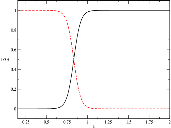
Figure 1: Evolution of ratio $\Gamma/3H$ as a function of the scale factor for the model II (solid, black line) and model III (dashed, red line). In drawing the graphs we have taken $\beta=0.1$.

Inserting Eqs. (6), (7), (8), in (3), and integrating, we have

$$\rho_{dm}=\rho_{dm0}\,a^{-3(1-\beta)}$$ (9)

for model I and

$$\rho_{dm}=\rho_{dm0}\,a^{-3}\,\exp\Big{(}3\beta\int_{1}^{a}\frac{g(\tilde{a})}{\tilde{a}}d\tilde{a}\Big{)}$$ (10)

for the two other models, with $g(a)=5\,-\,5\tanh(10-12a)$ and $g(a)=5\,-\,5\tanh(12a-10)$ for models II and III, respectively. In both cases, $g(a)/a\rightarrow 0$ as $a\rightarrow\infty$, whence the integral stays finite in that limit.

In terms of the redshift, $z=a^{-1}-1$, the Hubble expansion rate reads

$$\frac{H^{2}(z)}{H^{2}_{0}}=\Omega_{b0}\,(1+z)^{3}\,+\,\Omega_{dm0}\,(1+z)^{3(1-\beta)}\,+\,\Omega_{\Lambda 0}$$ (11)

for the model I and

$$\frac{H^{2}(z)}{H^{2}_{0}}=\Omega_{b0}\,(1+z)^{3}\,+\,\Omega_{dm0}\,(1+z)^{3}\,\exp\Big{(}-3\beta\int_{0}^{z}\frac{g(\tilde{z})}{(1+\tilde{z})}d\tilde{z}\Big{)}\,+\,\Omega_{\Lambda 0},$$ (12)

for models II and III, where the $\Omega_{i0}$ denote the current fractional densities of baryons, dark matter, and vacuum, and we have taken into account that the baryon energy density scales as $\,(1+z)^{3}$. Here and throughout the scale factor is normalized so that $\,a_{0}=1$.

IV Observational Constraints

To constrain the free parameters $\theta_{i}=(\beta,\Omega_{dm0})$ of the models above, we use 580 Supernova type Ia data points in the redshift interval $0.015\leq z\leq 1.41$ of the Union 2.1 compilation SNIa , 9 gamma-ray bursts in the redshift interval $1.54<z<3.5$ GRB2 , 6 points of baryon acoustic oscillations in the redshift interval $0.106\leq z\leq 0.730$ BAO , and 28 data points of the Hubble rate in the redshift interval $0.09<z<1.75$ Hz . Their best fit values, with their corresponding $1\sigma$ uncertainties, are presented in SEct. V. These follow from minimizing the likelihood function $L\propto\exp(-\chi_{total}^{2}/2)$ with $\chi^{2}_{total}=\chi^{2}_{SNIa}+\chi^{2}_{GRB}+\chi^{2}_{BAO}+\chi^{2}_{H}$, where each $\chi_{i}^{2}$ (specified below) quantifies the discrepancy between theory and observation. We not use the popular CMB shift parameter due to its comparative heavy dependence on the standard cold matter and $\Lambda$CDM models.

IV.1 Supernovae type Ia

Data from SN Ia are an important tool for understanding the recent evolution of the Universe. Here, we use the Union 2.1 compilation SNIa , available at http://supernova.lbl.gov/Union, that contains 580 SN Ia data in the redshift range $0.015\leq z\leq 1.41$. The distance modulus predicted for a given supernova of redshift $z$ can be expressed as

$$\mu_{th}(z)=5\log_{10}\left(\frac{D_{L}}{10{\rm pc}}\right)\,+\,\mu_{0}\,,$$ (13)

where $D_{L}=(1+z)\int_{0}^{z}{dz^{\prime}\,\frac{H_{0}}{H(z^{\prime})}}$ is the Hubble-free luminosity distance and $\mu_{0}=42.384-5\log_{10}h$, with $\,h=H_{0}/(100{\rm Km/s/Mpc})$, the reduced Hubble constant.

Assuming the SN Ia data follow a Gaussian distribution, we have

$$\chi^{2}_{SNIa}(\theta_{i},\mu_{0})=\sum_{i=1}^{580}\frac{[\mu^{obs}(z_{i})-\mu^{th}(z_{i},\theta_{i},\mu_{0})]^{2}}{\sigma^{2}(z_{i})},$$ (14)

where $\mu^{obs}$ denote the observed value, $\mu^{th}$ denote the value predicted by the model, $\theta_{i}=(\beta,\Omega_{dm0})$, and $\sigma_{i}$ stands for the 1$\sigma$ uncertainty associated to the $i$th data point. To eliminate the effect of the nuisance parameter $\mu_{0}$, which is independent of the data points and the data set, we minimize the right-hand side of the last equation with respect to $\mu_{0}$ following the procedure of Ref. prd_nesseris . We first expand $\chi^{2}$ in terms of $\mu_{0}$ as

$$\chi^{2}(\theta_{i})=A\,-\,\mu_{0}\,B\,+\,\mu_{0}^{2}\,C\,,$$ (15)

where

$$A(\theta_{i})=\sum_{i=1}^{580}\frac{[\mu^{obs}(z_{i})-\mu^{th}(z_{i},\theta_{i},\mu_{0}=0)]^{2}}{\sigma^{2}(z_{i})},$$ (16)

$$B(\theta_{i})=\sum_{i=1}^{580}\frac{[\mu^{obs}(z_{i})-\mu^{th}(z_{i},\theta_{i},\mu_{0}=0)]}{\sigma^{2}(z_{i})},$$ (17)

and

$$C=\sum_{i=1}^{580}\frac{1}{\sigma^{2}(z_{i})}.$$ (18)

Equation (15) presents a minimum for $\mu_{0}=B/C$ at

$$\tilde{\chi}^{2}(\theta_{i})=A(\theta_{i})\,-\,\frac{B^{2}(\theta_{i})}{C}.$$ (19)

Thus, rather than minimizing $\chi^{2}(\mu_{0},\theta_{i})$ we minimize $\tilde{\chi}^{2}(\theta_{i})$ that is independent of $\mu_{0}$. Clearly, $\chi^{2}_{{\rm min}}=\tilde{\chi}^{2}_{{\rm min}}$. Thus the Hubble constant, $H_{0}$, does not enter the calculation of the cosmological parameters when using SN Ia data.

In our analysis we have not taken into account the small correlations between the SN Ia data points. As seen in the paper by Conley et al. Conley , the correlations induced by systematic errors have a very minor impact (see, e.g., Fig. 11 in that paper). This was also found by Ruiz et al., prd_Ruiz (see, e.g., Fig. 11 there). We feel therefore confident that they will not significantly alter the overall result of our analysis (i.e., that, as argued below, models I and II may well explain the value of less than -1 reported in Refs. [2-5] for the EoS of dark energy.)

IV.2 Gamma-ray bursts

Gamma-ray bursts (GRBs) are very energetic astrophysical outbursts usually at higher redshifts than SN Ia events. Unfortunately, very often, GRBs are not standard candles as is the case of SN Ia. Therefore, it becomes necessary to calibrate them if they are to be employed as useful distance indicators. The uncertainties in the observable quantities of GRBs are much higher than in SNs Ia, since so far there is not a good understanding of their source mechanism. These issues favor a controversy over the use of GRBs for cosmological applications GRB1 .

Recently, in Ref. GRB2 , a set of 9 long gamma-ray bursts (LGRBs) in the redshift interval $1.54<z<3.5$ was calibrated through the type I fundamental plane. This is defined by the correlation between the spectral peak energy $E_{p}$, the peak luminosity $L_{p}$, and the luminosity time $T_{L}\equiv E_{iso}/L_{p}$, where $E_{iso}$ is the isotropic energy. This calibration is one of the different proposals to calibrate GRBs in an model cosmological-independent way. The fact that a control of systematic errors has been carried out to calibrate these 9 LGRBs GRB2 makes this compilation compelling.

The $\chi^{2}$ function for the GRB data reads

$$\chi^{2}_{GRB}(\theta_{i},\mu_{0})=\sum_{i=1}^{9}\frac{[\mu^{obs}(z_{i})-\mu^{th}(z_{i},\theta_{i},\mu_{0})]^{2}}{\sigma^{2}(z_{i})}.$$ (20)

Here, we perform the same procedure described in the previous section.

IV.3 Baryon acoustic oscillations

These can be traced to pressure waves at the recombination epoch generated by cosmological perturbations in the primeval baryon-photon plasma and appear as distinct peaks in the large-scale correlation function.

For the BAO measurements, we use the six estimates of the BAO parameter

$$A(z)=\sqrt{\Omega_{b}\,+\,\Omega_{dm}}\Big{[}\frac{r^{2}(z)}{z^{2}E(z)}\Big{]}^{1/3}$$ (21)

given in Table 3 of Ref. BAO , that are in the redshift range $0.106\leq z\leq 0.730$, which is the $H_{0}$ independent. In this expression, $r$ is the comoving distance.

The $\chi^{2}$ function for the BAO data is

$$\chi^{2}_{BAO}(z,\theta_{i})=\sum_{i=1}^{6}\frac{[A^{obs}(z_{i})-A^{th}(z_{i},\theta_{i})]^{2}}{\sigma^{2}_{BAO}(z_{i})}.$$ (22)

Again, we neglect the correlations in the BAO data as their impact in the final results is expected to be rather small (see, e.g., Fig 11 in Ref. prd_Ruiz ).

IV.4 History of the Hubble parameter

The differential evolution of early type passive galaxies provides direct information about the Hubble parameter, $H(z)$. An updated compilation of 28 data points $H(z)$ lying in the redshift interval $0.09<z<1.75$ can be found in Ref. Hz . Here, we use these data to constrain the cosmological free parameters $\theta_{i}$ of the three models under consideration.

We compute the $\chi^{2}_{H}$ function defined as

$$\chi^{2}_{H}(\theta_{i},H_{0})=\sum_{i=1}^{28}\frac{[H^{obs}(z_{i})-H^{th}(z_{i},H_{0},\theta_{i})]^{2}}{\sigma^{2}_{H}(z_{i})},$$ (23)

where $H_{th}(z_{i},H_{0},\theta_{i})$ is the model-predicted value of the Hubble parameter at the redshift $z_{i}$. This equation can be recast as

$$\chi^{2}_{H}(\theta_{i},H_{0})=H^{2}_{0}\sum_{i=1}^{28}\frac{E^{2}(z_{i},\theta)}{\sigma^{2}_{i}}-2H_{0}\sum_{i=1}^{28}\frac{H_{obs}(z_{i})E(z_{i},\theta)}{\sigma^{2}_{i}}+\frac{H^{2}_{obs}(z_{i})}{\sigma^{2}_{i}}.$$ (24)

The $\chi^{2}_{H}$ function depends on the model parameters $\theta_{i}$ as well as on the nuisance parameter $H_{0}$, the value of which is not very well known. To marginalize over the latter, we assume that the distribution of $H_{0}$ is Gaussian with standard deviation width $\sigma_{H_{0}}$ and mean ${\bar{H}_{0}}$. Then, we build the posterior likelihood function $L_{H}(\theta)$ that depends just on the free parameters $\theta_{i}$,

$$L_{H}=\int\pi_{H}(H_{0})e^{-\chi^{2}_{H}(H_{0},\theta_{i})}dH_{0},$$ (25)

where

$$\pi_{H}(H_{0})=\frac{1}{\sqrt{2\pi}\sigma_{H_{0}}}e^{-(H_{0}-\bar{H}_{0})^{2}/2\sigma^{2}_{H_{0}}}\,,$$ (26)

is a prior probability function widely used in the literature. For ${\bar{H}_{0}}$, we take the best-fit value provided by Riess et al. Riess . Finally, we minimize $\chi^{2}_{H}(\theta_{i})=-2\ln L_{H}(\theta_{i})$ with respect to the free parameters $\theta_{i}$ to obtain the best-fit parameter values.

V Results

Tables 1 and 2 summarize the main results of the statistical analysis carried out using the set of data, SNIa+GRB+BAO and SNIa+GRB+BAO+$H(z)$, respectively.

Figure 2 shows the $68\%$ and $95\%$ confidence contours in the plane $\beta-\Omega_{dm0}$ for model I considering the sets of data SNIa+GRB+BAO (left panel), and SNIa+GRB+BAO+$H(z)$ (right panel). Although the best fit for $\beta$ is small for the two cases, the possibility of a small creation rate ($\beta>0$ $\Rightarrow$ $\Gamma>0$) is not ruled out. In fact, $0\leq\beta\leq 0.093$ and $0\leq\beta\leq 0.136$ at 1$\sigma$ and 2$\sigma$ confidence levels, respectively, for SNIa+GRB+BAO, and $0.039\leq\beta\leq 0.108$ ($0.017\leq\beta\leq 0.130$) in 1$\sigma$ (2$\sigma$) when we considered SNIa+GRB+BAO+$H(z)$. We see that a nonzero creation rate ($\Gamma>0$) is consistent with the set data SNIa+GRB+BAO+$H(z)$ in $1\sigma$ and $2\sigma$, and from this analysis, we obtained $w_{eff}(z=0)=-1.073^{+0.034}_{-0.035}$ in $1\sigma$ of statistical confidence. For the joint analysis SNIa+GRB+BAO, we have an effective EoS, $w_{eff}(z=0)=-1.0249^{+0.0249}_{-0.0691}$. This hints that the combined effect of the quantum vacuum and the particle creation rate may indeed result in an effective EoS lower than $-1$. The associated uncertainty of $w_{eff}$ was determined by using the standard error propagation method.

	$\beta$	$\Omega_{dm0}$	$\chi^{2}_{min}/dof$
Model I, Eq. (6),	$0.025^{+0.068}_{-0.065}$	$\;\,0.237^{+0.016}_{-0.015}$	$\;0.9589$
Model II, Eq. (7),	$0.03^{+0.081}_{-0.069}$	$\;\,0.251^{+0.016}_{-0.016}$	$\;0.9587$
Model III, Eq. (8),	$0.003^{+0.007}_{-0.006}$	$\;\,0.251^{+0.017}_{-0.016}$	$\;0.9590$

Table 1: Best-fit values with their $1\sigma$ errors of the free parameters, $\beta$ and $\Omega_{dm0}$, for the three models considered in this work obtained from joint analysis SNIa+GRB+BAO.

	$\beta$	$\Omega_{dm0}$	$\chi^{2}_{min}/dof$
Model I, Eq. (6),	$0.0729^{+0.035}_{-0.034}$	$\;\,0.232^{+0.016}_{-0.015}$	$\;0.9549$
Model II, Eq. (7),	$0.0158^{+0.0082}_{-0.0077}$	$\;\,0.233^{+0.015}_{-0.014}$	$\>0.9774$
Model III, Eq. (8),	$0.0127^{+0.0049}_{-0.0050}$	$\;\,0.240^{+0.016}_{-0.015}$	$\;0.9705$

Table 2: Best-fit values with their $1\sigma$ errors of the free parameters, $\beta$ and $\Omega_{dm0}$, for the three models considered in this work obtained from the joint analysis SNIa+GRB+BAO+$H(z)$.

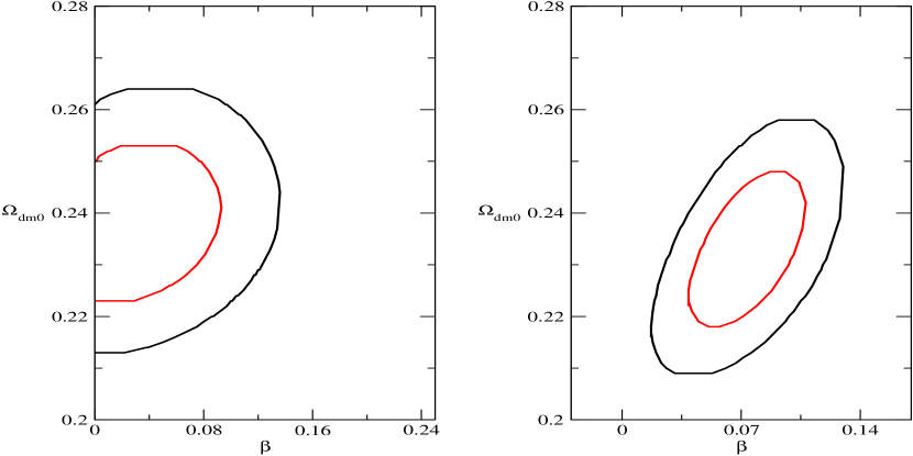
Figure 2: Left panel: 1$\sigma$ and 2$\sigma$ confidence contours for model I obtained from joint analysis SNIa+GRB+BAO. Right panel: The same but using the set of data SNIa+GRB+BAO+$H(z)$.

Figures 3 and 4 show the $68\%$ and $95\%$ confidence contours in the $\beta-\Omega_{dm0}$ plan for models II (left panel), and the evolution of $w_{eff}$ in 1$\sigma$ (right panel) for the respective data sets, SNIa+GRB+BAO, and SNIa+GRB+BAO+$H(z)$. As can be observed, the inclusion of the data set, $H(z)$, significantly reduces the constraints on the parameter $\beta$, since it, changed from $0\leq\beta\leq 0.111$ to $0.0081\leq\beta\leq 0.024$ in 1$\sigma$, for example. This scenario, presents as effective EoS, $w_{eff}(z=0)=-1.2944^{+0.2944}_{-0.8049}$ for the analysis with SNIa+GRB+BAO, and $w_{eff}(z=0)=-1.555^{+0.076}_{-0.080}$ for SNIa+GRB+BAO+$H(z)$, both in 1$\sigma$. This model, which is characterized by a production rate of particles that grow throughout cosmic history, today presents a significant effective EoS phantom. Figures 5 and 6 show the $68\%$ and $95\%$ confidence contours in the $\beta-\Omega_{dm0}$ plan for models III (left panel) and the evolution of $w_{eff}$ in 1$\sigma$ (right panel) for the respective data sets, SNIa+GRB+BAO and SNIa+GRB+BAO+$H(z)$. Here, we have that the model presents a small effective EoS in the present moment, being $w_{eff}(z=0)=-1^{+0}_{-0.0018}$ for SNIa+GRB+BAO and
$w_{eff}(z=0)=-1.002^{+0.001}_{-0.001}$ for SNIa+GRB+BAO+$H(z)$.

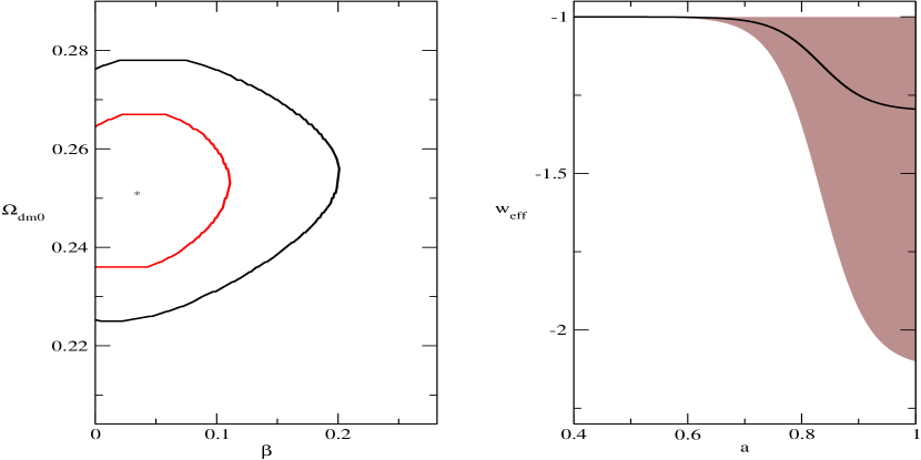
Figure 3: Left panel: 1$\sigma$ and 2$\sigma$ confidence contours for model II obtained from the joint analysis SNIa+GRB+BAO. Right panel: Evolution of the effective EoS in terms of the scale factor; the solid (black) line indicates the best-fit values, and the shaded region indicates the $1\sigma$ uncertainty.

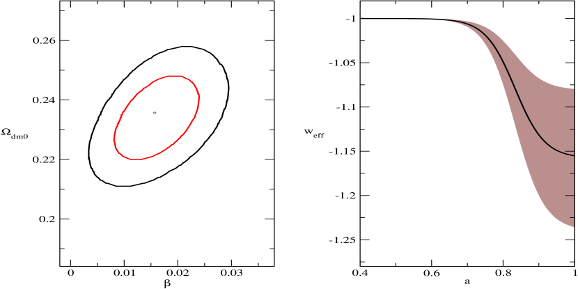
Figure 4: Same as Fig. 3 but using the set of data SNIa+GRB+BAO+$H(z)$.

Figure 5: Left panel: 1$\sigma$ and 2$\sigma$ confidence contours for model III obtained from joint analysis SNIa+GRB+BAO. Right panel: Evolution of the effective EoS in terms of the scale factor; the solid (black) line indicates the best-fit values, and the shaded region indicates the $1\sigma$ uncertainty.

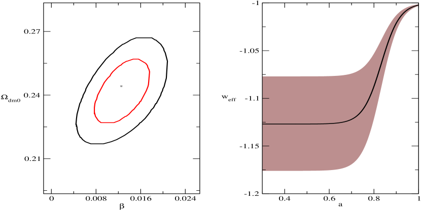
Figure 6: Same as Fig. 5 but using the set of data SNIa+GRB+BAO+$H(z)$.

To sum up, after constraining the three models proposed in this work with the set of observational data specified in Sec. IV it is seen first that, as a result of the joint effect of the vacuum and the particle creation rate, effective equations of state of phantom type can be obtained at present time and in the past.

VI Comparison with models of coupled dark energy

At this point one may wonder whether models of DE featuring a nongravitational coupling with dark matter may also lead to an effective EoS of phantom type. As we will see, the answer is they very likely will not.

The said models were proposed to lower the value of the cosmological constant aa-wetterich and to solve or, at least, alleviate the coincidence problem (“why are the densities of dark energy and dark matter of the same order precisely today?”); see, e.g., Ref. coupled . In any case, a coupling between the dark components seems natural, though it must be small as it is severely constrained by observations -see signpost for a review.

For a spatially flat, homogeneous, and isotropic universe, these models are characterized by the set of equations

$$\dot{\rho}_{b}\, + \,3H\rho_{b}=0\,,$$ (27)

$$\dot{\rho}_{dm}\, + \,3H\rho_{dm}=Q\,,$$ (28)

$$\dot{\rho}_{de}\, + \,3H(1+w)\rho_{de}=-Q\,,$$ (29)

$$3H^{2} = 8\pi G(\rho_{b}\,+\,\rho_{dm}\,+\,\rho_{de})\,,$$ (30)

where $Q$ stands for the energy transfer rate per unit of volume between the dark components and the EoS of DE is bounded by $-1\leq w<-1/3$. This class of models implicitly assumes that the creation pressure either vanishes or is negligible. Because of the interaction, the energy density of DM, $\rho_{dm}=n\,m$, differs from the usual conservation expression, $\rho_{dm}=\rho_{dm0}\,a^{-3}$, either because $\,m\,$ varies with expansion or because the number density of DM particles does not obey the expression $n=n_{0}\,a^{-3}$.

Two distinct possibilities arise: (i) $Q>0$, which means a continuous transfer of energy from DE to DM, and (ii) $Q<0$ in this case, the transfer of energy would proceed in the opposite sense. For $Q>0$, the effective EoS, $w_{eff}=w+Q/(3H\rho_{dm})$, results less negative than $w$, and thereby no phantom behavior can be reproduced (this holds irrespective of whether it is the number or mass of DM particles that varies).

For $Q<0$, one follows that $w_{eff}$ can be less than $-1$. However this kind of model can be readily told apart from the ones discussed in the above sections. In particle creation models, DM particles are continuously added to this pressureless component, and thereby the amount of DM in the past is necessarily less, at any $z>0$, than (at the same redshift) in the $\Lambda$CDM model that shares the same $\Omega_{b0}$ and $\Omega_{dm0}$ than the matter creation model. Likewise, in coupled models with $Q<0$ the amount of DM in the past was certainly larger, at any $z>0$, than (at the same redshift) in the $\Lambda$CDM model with identical $\Omega_{b0}$ and $\Omega_{dm0}$. Consequently, the growth function, $f_{g}\equiv{\rm d}\ln D_{+}/{\rm d}\ln a$, in matter creation models is greater than in the $\Lambda$CDM and $f_{g}$ is also greater in the $\Lambda$CDM than in the said kind of coupled models.

Further, as is well known, the transfer of energy from DM to DE worsens the coincidence problem and violates the second law of thermodynamics grg-db , and the conservation of quantum numbers could be transgressed, especially if DE is the quantum vacuum.

In summary, models of coupled dark energy clearly differentiate observationally from creation models, and it is very unlikely that they can reproduce the EoS of phantom models.

VII Concluding remarks

Current observational data seem to favor an EoS for DE less than $-1$ (for a quick summary of the state of art, see Fig. 1 in Ref. Shafer ). If confirmed by future experiments, like Euclide euclide , we will confront the puzzling situation that the current expansion stage of the Universe is likely driven by a phantom field, in spite of the fact that these fields are known to come with theoretical drawbacks of no easy fixing.

In this paper we explored the possibility that the $\,w_{de}$ determined by recent experiments is in reality an effective EoS that results from adding the negative EoS, $w_{c}=-\Gamma/3H$ (associated to the particle production pressure from the gravitational field acting on the vacuum, Parker , Lima1 ), to the EoS of the vacuum itself, $w_{\Lambda}=-1$. Since the rate of particle production, $\Gamma$, is not known, we have assumed three different phenomenological Ansätze for the latter on grounds of simplicity, Eqs. (6)-(8), and constrained their free parameters ($\beta$ and $\Omega_{dm0}$) of the corresponding cosmological models with the combinations SN Ia + GRBs + BAO and SN Ia + GRBs + BAO + H(z) of observational data sets. Here we wish to stress that we did not fix the value of the Hubble constant, $H_{0}$, at any point in the statistical analysis. As it turns out, models I and II suggest that the pressure of the vacuum combined with the particle creation pressure helps explain that the EoS measured by recent experiments (see, e.g., Refs. Rest -Shafer ) is less than $-1$. Model III lies far away from explaining it.

To sum up, the recently reported values of lower than $-1$ for the equation of state of dark energy may arise from the joint effect of the quantum vacuum and the process of particle production. This offers a viable alternative to the embarrassing possibility of fields that, among other things, violate the dominant energy condition, give rise to classical and quantum instabilities, and do not respect the second law of thermodynamics.

Obviously, phenomenological models of particle production different from the ones essayed here are also worth exploring. More important, however, is to determine the rate $\Gamma$ using quantum field theory but, as said above, this does not seem feasible until the nature of DM particles is found.

- (1) P.A.R. Ade et al. (Planck Collaboration), “Planck 2013 results. XVI. Cosmological parameters”, Astron. Astrophys 571, A16 (2014).
- (2) A. Rest et al., “Cosmological constraints from measurements of type Ia supernovae discovered during the first years of the Pan-STARRS1 Survey”, Astrophys. J. 795,, no 1, 44 (2014).
- (3) J.-Q. Xia, H. Li, and X. Zhang, Phys. Rev. D 88, 063501 (2013).
- (4) C. Cheng, and Q.-G Huang, Phys. Rev. D 89, 043003 (2014).
- (5) D.L. Shafer and D. Huterer, Phys. Rev. D 89, 063510 (2014).
- (6) A. Conley et al., Astrophys. J. Suppl. Ser. 192, 1 (2011).
- (7) D. Scolnic et al., “Systematic uncertainties associated with the cosmological analysis of the first Pan-STARRS1 type Ia supernova sample”, Astrophys. J. 795, no 1, 45 (2014).
- (8) R.R. Caldwell, Phys. Lett. B 545, 23 (2002).
- (9) S.M. Carroll, M. Hoffman and M. Trodden, Phys. Rev. D 68, 023509 (2003).
- (10) J.M. Cline, S. Jeon and G. D. Moore, Phys. Rev. D 70, 86 043543 (2004).
- (11) S.D.H. Hsu, A. Jenkins, and M.B. Wise, Phys. Lett. B 597, 270 (2004).
- (12) F. Sbisa, Eur. J. Phys. 36, 015009 (2015).
- (13) M. Dabrowski, arXiv:1411.2827.
- (14) L. Parker, Fund. Cosm. Phys. 7, 201 (1982); L. Parker, Phys. Rev. Lett., 21, 562 (1968); L. Parker, Phys. Rev. Lett. 183, 1057 (1966); S.A. Fulling, L. Parker, and B.L. Hu, Phys. Rev. D, 10, 3905 (1974); L. Parker, Phys. Rev. D 17, 933 (1978); N.J. Paspatamatiou, and L. Parker, Phys. Rev. D 19, 2283 (1979).
- (15) I. Prigogine, J. Geheniau, E. Gunzig, and P. Nardone, General. Relativ. Gravit. 21, 767 (1989).
- (16) L.E. Parker and D.J. Toms, Quantum Field Theory in Curved Spacetime: Quantized Fields and Gravity (Cambridge University Press, England, 2009).
- (17) J.A.S. Lima, M.O. Calvão, and I. Waga, Cosmology, Thermodynamics and Matter Creation, Frontier Physics, Essays in Honor of Jayme Tiomno (World Scientific, Singapore, 1990); M.O. Calvão, J.A.S. Lima, and I. Waga, Phys. Lett. A 162, 223 (1992); J.A.S. Lima, A.S.M. Germano, and L.R.W. Abramo, Phys. Rev. D 53, 4287 (1996).
- (18) W. Zimdahl and D. Pavón, Mon. Not. R. Astron. Soc. 266, 872 (1994).
- (19) W. Zimdahl, D.J. Schwarz, A.B. Balakin, and D. Pavón, Phys. Rev. D 64, 063501, (2001).
- (20) J. Triginer, W. Zimdahl, and D. Pavón, Class. Quantum Grav. 13, 403 (1996).
- (21) J.A.S. Lima and I. Baranov, Phys. Rev. D 90, 043515 (2014).
- (22) J. Ellis, S. Kalara, K.A. Olive, C. Wetterich, Phys. Lett. B 228, 264 (1989).
- (23) P.J.E. Peebles and B. Ratra, Rev. Mod. Phys. 75, 559 (2003).
- (24) K. Hagiwara et al. [Particle Data Group], Phys. Rev. D. 66, 010001(R) (2002).
- (25) N. Suzuki et al. [The Supernova Cosmology Project], Astrophys. J. 746, 85 (2012); http://supernova.lbl.gov/Union/.
- (26) H.J. Mosquera Cuesta, H. Dumet, and C. Furlanetto, JCAP 07(2008)004; N. Liang, P. Wu, and S.N. Zhang, Phys. Rev. D 81, 083518 (2010); C. Graziani, New Astron. 16, 57 (2011); A. Shahmoradi and R. Nemiroff, Mon. Not. R. Astron. Soc. 411 1843 (2011); N.R. Butler, J.S. Bloom, D. Poznanski, Astrophys. J. 711, 495 (2010).
- (27) R. Tsutsui et al., arXiv:1205.2954.
- (28) C. Blake et al., Mon. Not. R. Astron. Soc. 418, 1707 (2011).
- (29) K. Liao, Z. Li, J. Ming, and Z.-H. Zhu, Phys. Lett. B 718, 1166 (2013).
- (30) S. Nesseris and L. Perivolaropoulos, Phys. Rev. D 72, 123519 (2005).
- (31) E.J. Ruiz, D.L. Shafer, D. Huterer, and A Conley, Phys. Rev. D 86, 103004 (2012).
- (32) A. G. Riess et al., Astrophys. J. 730, 119 (2011).
- (33) C. Wetterich, Astron. Astrophysics 301, 321 (1995).
- (34) L. Amendola, Phys. Rev. D 62, 043511 (2000); L.P. Chimento, A. Jakubi, D. Pavón, and W. Zimdahl, Phys. Rev. D 67, 083513 (2003); A.A. Costa et al., Phys. Rev. D 89, 103531 (2014); E. Abdalla, E.G.M. Ferreira, J. Quintin, and B. Wang, arXiv:1412.2777.
- (35) F. Atrio-Barandela and D. Pavón, “Interacting dark energy”, in Dark Energy -Current Advances and Ideas, ed. J.R. Choi (Research Signpost, Trivandrum, India, 2009).
- (36) D. Pavón and B. Wang, General Relativ. Gravit. 41, 1 (2009).
- (37) http://www.euclid-ec.org.