Algorithms and complexity for
Turaev-Viro invariants

Abstract

The Turaev-Viro invariants are a powerful family of topological invariants for distinguishing between different 3-manifolds. They are invaluable for mathematical software, but current algorithms to compute them require exponential time.

The invariants are parameterised by an integer $r\geq 3$. We resolve the question of complexity for $r=3$ and $r=4$, giving simple proofs that computing Turaev-Viro invariants for $r=3$ is polynomial time, but for $r=4$ is #P-hard. Moreover, we give an explicit fixed-parameter tractable algorithm for arbitrary $r$, and show through concrete implementation and experimentation that this algorithm is practical—and indeed preferable—to the prior state of the art for real computation.

Keywords: Computational topology, 3-manifolds, invariants, #P-hardness, parameterised complexity

1 Introduction

In geometric topology, testing homeomorphism (topological equivalence) is a fundamental algorithmic problem. However, beyond dimension two it is remarkably difficult. In dimension three—the focus of this paper—an algorithm follows from Perelman’s proof of the geometrisation conjecture [12], but it is extremely intricate, its complexity is unknown and it has never been implemented.

As a result, practitioners in computational topology rely on simpler topological invariants—computable properties of a topological space that can be used to tell different spaces apart. One of the best known invariants is homology, but for 3-manifolds (the 3-dimensional generalisation of surfaces) this is weak: there are many topologically different 3-manifolds that homology cannot distinguish. Therefore major software packages in 3-manifold topology rely on invariants that are stronger but more difficult to compute.

In the discrete setting, among the most useful invariants for 3-manifolds are the Turaev-Viro invariants [19]. These are analogous to the Jones polynomial for knots: they derive from quantum field theory, but offer a much simpler combinatorial interpretation that lends itself well to algorithms and exact computation. They are implemented in the major software packages Regina [5] and the Manifold Recogniser [14, 15], and they play a key role in developing census databases, which are analogous to the well-known dictionaries of knots [3, 14]. Their main difficulty is that they are slow to compute: current implementations [5, 15] are based on backtracking searches, and require exponential time.

The purpose of this paper is threefold: (i) to introduce the Turaev-Viro invariants to the wider computational topology community; (ii) to understand the complexity of computing these invariants; and (iii) to develop new algorithms that are suitable for practical software.

The Turaev-Viro invariants are parameterised by two integers $r$ and $q$, with $r\geq 3$; we denote these invariants by $\mathrm{TV}_{r,q}$. A typical algorithm for computing $\mathrm{TV}_{r,q}$ will take as input a triangulated 3-manifold, composed of $n$ tetrahedra attached along their triangular faces; we use $n$ to indicate the input size. For all known algorithms, the difficulty of computing $\mathrm{TV}_{r,q}$ grows significantly as $r$ increases (but in contrast, the difficulty is essentially independent of $q$).

Our main results are as follows.

• Kauffman and Lins [9] state that for $r=3,4$ one can compute $\mathrm{TV}_{r,q}$ via “simple and efficient methods of linear algebra”, but they give no details on either the algorithms or the complexity. We show here that in fact the situations for $r=3$ and $r=4$ are markedly different: computing $\mathrm{TV}_{r,q}$ for orientable manifolds and $r=3$ is polynomial time, but for $r=4$ is #P-hard.

• We give an explicit algorithm for computing $\mathrm{TV}_{r,q}$ for general $r$ that is fixed-parameter tractable (FPT). Specifically, for any fixed $r$ and any class of input triangulations whose dual graphs have bounded treewidth, the algorithm has running time linear in $n$. Furthermore, we show through comprehensive experimentation that this algorithm is practical—we implement it in the open-source software package Regina [5], run it through exhaustive census databases, and find that this new FPT algorithm is comparable to—and often significantly faster than—the prior backtracking algorithm.

• We give a new geometric interpretation of the formula for $\mathrm{TV}_{r,q}$, based on systems of “normal arcs” in triangles. This generalises earlier observations of Kauffman and Lins for $r=3$ based on embedded surfaces [9], and offers an interesting potential for future algorithms based on Hilbert bases.

The #P-hardness result for $r=4$ is the first classical hardness result for the Turaev-Viro invariants. However, the proofs for this and the polynomial-time $r=3$ result are simple: the algorithm for $r=3$ derives from a known homological formulation [14], and the result for $r=4$ adapts Kirby and Melvin’s NP-hardness proof for the more complex Witten-Reshetikhin-Turaev invariants [10].

The FPT algorithm for general $r$ is significant in that it is not just theoretical, but also practical—and indeed preferable—for real software. It was previously known that computing $\mathrm{TV}_{r,q}$ is FPT [6], but that prior result was purely existential, and would lead to infeasibly large constants in the running time if translated to a concrete algorithm. More generally, FPT algorithms do not always translate well into practical software tools, and this paper is significant in giving the first demonstrably practical FPT algorithm in 3-manifold topology.

2 Preliminaries

Let $M$ be a closed 3-manifold. A generalised triangulation of $M$ is a collection of $n$ abstract tetrahedra $\Delta_{1},\ldots,\Delta_{n}$ equipped with affine maps that identify (or “glue together”) their $4n$ triangular faces in pairs, so that the underlying topological space is homeomorphic to $M$.

In particular, as a consequence of the face identifications, it is possible that several vertices of the same tetrahedron may be identified together (and likewise for edges and triangles). Indeed, it is common in practical applications to have a one-vertex triangulation, in which all vertices of all tetrahedra are identified to a common point. In general, the $4n$ tetrahedron vertices are partitioned into equivalence classes according to how they are identified together; we refer to each such equivalence class as a single vertex of the triangulation, and likewise for edges and triangles.

Generalised triangulations are widely used across major 3-manifold software packages. They are (as the name suggests) more general than simplicial complexes, which allows them to express a rich variety of different 3-manifolds using very few tetrahedra. For instance, with just $n\leq 11$ tetrahedra one can create 13 400 distinct prime orientable 3-manifolds [4, 14].

2.1 The Turaev-Viro invariants

Let $\mathfrak{T}$ be a generalised triangulation of a closed 3-manifold $M$, and let $r$ and $q$ be integers with $r\geq 3$, $0<q<2r$, and $\gcd(r,q)=1$. We define the Turaev-Viro invariant $\mathrm{TV}_{r,q}(\mathfrak{T})$ as follows.

Let $V$, $E$, $F$ and $T$ denote the set of vertices, edges, triangles and tetrahedra respectively of the triangulation $\mathfrak{T}$. Let $I=\{0,1/2,1,3/2,\ldots,(r-2)/2\}$; note that $|I|=r-1$. We define a colouring of $\mathfrak{T}$ to be a map $\theta\colon\thinspace E\to I$; that is, $\theta$ “colours” each edge of $\mathfrak{T}$ with an element of $I$. A colouring $\theta$ is admissible if, for each triangle of $\mathfrak{T}$, the three edges $e_{1}$, $e_{2}$, and $e_{3}$ bounding the triangle satisfy:

• the parity condition $\theta(e_{1})+\theta(e_{2})+\theta(e_{3})\in\mathbb{Z}$;

• the triangle inequalities $\theta(e_{1})\leq\theta(e_{2})+\theta(e_{3})$, $\theta(e_{2})\leq\theta(e_{1})+\theta(e_{3})$, and $\theta(e_{3})\leq\theta(e_{1})+\theta(e_{2})$; and

• the upper bound constraint $\theta(e_{1})+\theta(e_{2})+\theta(e_{3})\leq r-2$.

More generally, we refer to any triple $(i,j,k)\in I\times I\times I$ satisfying these three conditions as an admissible triple of colours.

For each admissible colouring $\theta$ and for each vertex $v\in V$, edge $e\in E$, triangle $f\in F$ or tetrahedron $t\in T$, we define weights $|v|_{\theta},|e|_{\theta},|f|_{\theta},|t|_{\theta}\in\mathbb{C}$.

Our notation differs slightly from Turaev and Viro [19]; most notably, Turaev and Viro do not consider triangle weights $|f|_{\theta}$, but instead incorporate an additional factor of $|f|_{\theta}^{1/2}$ into each tetrahedron weight $|t|_{\theta}$ and $|t^{\prime}|_{\theta}$ for the two tetrahedra $t$ and $t^{\prime}$ containing $f$. This choice of notation simplifies the notation and avoids unnecessary (but harmless) ambiguities when taking square roots.

Let $\zeta=e^{i\pi q/r}\in\mathbb{C}$. Note that our conditions imply that $\zeta$ is a $(2r)$th root of unity, and that $\zeta^{2}$ is a primitive $r$th root of unity; that is, $(\zeta^{2})^{k}\neq 1$ for $k=1,\ldots,r-1$. For each positive integer $i$, we define $[i]=(\zeta^{i}-\zeta^{-i})/(\zeta-\zeta^{-1})$ and, as a special case, $[0]=1$. We next define the “bracket factorial” $[i]!=[i]\,[i-1]\ldots[0]$. Note that $[r]=0$, and thus $[i]!=0$ for all $i\geq r$.

We give every vertex constant weight

$$|v|_{\theta}=\frac{\left|\zeta-\zeta^{-1}\right|^{2}}{2r},$$

and to each edge $e$ of colour $i\in I$ (i.e., for which $\theta(e)=i$) we give the weight

$$|e|_{\theta}=(-1)^{2i}\cdot[2i+1].$$

A triangle $f$ whose three edges have colours $i,j,k\in I$ is assigned the weight

$$|f|_{\theta}=(-1)^{i+j+k}\cdot\frac{[i+j-k]!\cdot[i+k-j]!\cdot[j+k-i]!}{[i+j+k+1]!}.$$

Note that the parity condition and triangle inequalities ensure that the argument inside each bracket factorial is a non-negative integer.

Figure 1: Edge colours of a tetrahedron.

Finally, let $t$ be a tetrahedron with edge colours $i_{0},i_{1},i_{2},i_{3},i_{4},i_{5}$ as indicated in Figure 1. In particular, the four triangles surrounding $t$ have colours $(i_{0},i_{1},i_{3})$, $(i_{0},i_{2},i_{4})$, $(i_{1},i_{2},i_{5})$ and $(i_{3},i_{4},i_{5})$, and the three pairs of opposite edges have colours $(i_{0},i_{5})$, $(i_{1},i_{4})$ and $(i_{2},i_{3})$. We define

$$\tau_{\phi}(t,z) =[z-i_{0}-i_{1}-i_{3}]!\cdot[z-i_{0}-i_{2}-i_{4}]!\cdot[z-i_{1}-i_{2}-i_{5}]!\cdot[z-i_{3}-i_{4}-i_{5}]!\,,$$

$$\kappa_{\phi}(t,z) =[i_{0}+i_{1}+i_{4}+i_{5}-z]!\cdot[i_{0}+i_{2}+i_{3}+i_{5}-z]!\cdot[i_{1}+i_{2}+i_{3}+i_{4}-z]!$$

for all integers $z$ such that the bracket factorials above all have non-negative arguments; equivalently, for all integers $z$ in the range $z^{-}\leq z\leq z^{+}$ with

$$z^{-} =\max\{i_{0}+i_{1}+i_{3},\ i_{0}+i_{2}+i_{4},\ i_{1}+i_{2}+i_{5},\ i_{3}+i_{4}+i_{5}\}\,;$$

$$z^{+} =\min\{i_{0}+i_{1}+i_{4}+i_{5},\ i_{0}+i_{2}+i_{3}+i_{5},\ i_{1}+i_{2}+i_{3}+i_{4}\}.$$

Note that, as before, the parity condition ensures that the argument inside each bracket factorial above is an integer. We then declare the weight of tetrahedron $t$ to be

$$|t|_{\phi}=\sum_{z^{-}\leq z\leq z^{+}}\frac{(-1)^{z}\cdot[z+1]!}{\tau_{\phi}(t,z)\cdot\kappa_{\phi}(t,z)},$$

Note that all weights are polynomials on $\zeta$ with rational coefficients, where $\zeta=e^{i\pi q/r}$.

Using these weights, we define the weight of the colouring to be

$$|\mathfrak{T}|_{\theta}=\prod_{v\in V}|v|_{\theta}\times\prod_{e\in E}|e|_{\theta}\times\prod_{f\in F}|f|_{\theta}\times\prod_{t\in T}|t|_{\theta},$$ (1)

and the Turaev-Viro invariant to be the sum over all admissible colourings

$$\mathrm{TV}_{r,q}(\mathfrak{T})=\sum_{\theta\ \mathrm{admissible}}|\mathfrak{T}|_{\theta}.$$

In [19], Turaev and Viro show that $\mathrm{TV}_{r,q}(\mathfrak{T})$ is indeed an invariant of the manifold; that is, if $\mathfrak{T}$ and $\mathfrak{T}^{\prime}$ are generalised triangulations of the same closed 3-manifold $M$, then $\mathrm{TV}_{r,q}(\mathfrak{T})=\mathrm{TV}_{r,q}(\mathfrak{T}^{\prime})$ for all $r,q$. Although $\mathrm{TV}_{r,q}(\mathfrak{T})$ is defined on the complex numbers $\mathbb{C}$, it always takes a real value (more precisely, it is the square of the modulus of a Witten-Reshetikhin-Turaev invariant) [22].

2.2 Treewidth and parameterised complexity

Throughout this paper we always refer to nodes and arcs of graphs, to clearly distinguish these from the vertices and edges of triangulations.

Robertson and Seymour introduced the concept of the treewidth of a graph [17], which now plays a major role in parameterised complexity. Here, we adapt this concept to triangulations in a straightforward way.

Definition.

Let $\mathfrak{T}$ be a generalised triangulation of a 3-manifold, and let $T$ be the set of tetrahedra in $\mathfrak{T}$. A tree decomposition $(X,\{B_{\tau}\})$ of $\mathfrak{T}$ consists of a tree $X$ and bags $B_{\tau}\subseteq T$ for each node $\tau$ of $X$, for which:

• each tetrahedron $t\in T$ belongs to some bag $B_{\tau}$;

• if a face of some tetrahedron $t_{1}\in T$ is identified with a face of some other tetrahedron $t_{2}\in T$, then there exists a bag $B_{\tau}$ with $t_{1},t_{2}\in B_{\tau}$;

• for each tetrahedron $t\in T$, the bags containing $t$ correspond to a connected subtree of $X$.

The width of this tree decomposition is defined as $\max|B_{\tau}|-1$. The treewidth of $\mathfrak{T}$, denoted $\mathrm{tw}(\mathfrak{T})$, is the smallest width of any tree decomposition of $\mathfrak{T}$.

The relationship between this definition and the classical graph-theoretical notion of treewidth is simple: $\mathrm{tw}(\mathfrak{T})$ is the treewidth of the dual graph of $\mathfrak{T}$, the $4$-valent multigraph whose nodes correspond to tetrahedra of $\mathfrak{T}$ and whose arcs represent pairs of tetrahedron faces that are identified together.

Figure 2 shows the dual graph of a $9$-tetrahedra triangulation of a $3$-manifold, along with a possible tree decomposition. The largest bags have size three, and so the width of this tree decomposition is $3-1=2$.

Figure 2: The dual graph and a tree decomposition of a $3$-manifold triangulation

Definition.

A nice tree decomposition of a generalised triangulation $\mathfrak{T}$ is a tree decomposition $(X,\{B_{\tau}\})$ of $\mathfrak{T}$ whose underlying tree $X$ is rooted, and where:

• The bag $B_{\rho}$ at the root of the tree is empty ($B_{\rho}$ is called the root bag);

• If a bag $B_{\tau}$ has no children, then $|B_{\tau}|=1$ (such a $B_{\tau}$ is called a leaf bag);

• If a bag $B_{\tau}$ has two children $B_{\sigma}$ and $B_{\mu}$, then $B_{\tau}=B_{\sigma}=B_{\mu}$ (such a $B_{\tau}$ is called a join bag);

• Every other bag $B_{\tau}$ has precisely one child $B_{\sigma}$, and either:

  • $|B_{\tau}|=|B_{\sigma}|+1$ and $B_{\tau}\supset B_{\sigma}$ (such a $B_{\tau}$ is called an introduce bag), or

  • $|B_{\tau}|=|B_{\sigma}|-1$ and $B_{\tau}\subset B_{\sigma}$ (such a $B_{\tau}$ is called a forget bag).

Given a tree decomposition of a triangulation $\mathfrak{T}$ of width $k$ and $O(n)$ bags, we can convert this in $O(n)$ time into a nice tree decomposition of $\mathfrak{T}$ that also has width $w$ and $O(n)$ bags [13].

3 Algorithms for computing Turaev-Viro invariants

All of the algorithms in this paper use exact arithmetic. This is crucial if we wish to avoid floating-point numerical instability, since computing $\mathrm{TV}_{r,q}$ may involve exponentially many arithmetic operations.

We briefly describe how this exact arithmetic works. Since all weights in the definition of $\mathrm{TV}_{r,q}$ are rational polynomials in $\zeta=e^{i\pi q/r}$, all arithmetic operations remain within the rational field extension $\mathbb{Q}(\zeta)$. If $\zeta$ is a primitive $n$th root of unity then this field extension is called the $n$th cyclotomic field. This in turn is isomorphic to the polynomial field $\mathbb{Q}[X]/\Phi_{n}(X)$, where $\Phi_{n}(X)$ is the $n$th cyclotomic polynomial with degree $\varphi(n)$ (Euler’s totient function). Therefore we can implement exact arithmetic using degree $\varphi(n)$ polynomials over $\mathbb{Q}$.

If $r$ is odd and $q$ is even, then $\zeta$ is a primitive $r$th root of unity, and $\mathbb{Q}(\zeta)\cong\mathbb{Q}[X]/\Phi_{r}(X)$. Otherwise $\zeta$ is a primitive $(2r)$th root of unity, and $\mathbb{Q}(\zeta)\cong\mathbb{Q}[X]/\Phi_{2r}(X)$. In this paper we give our complexity results in terms of arithmetic operations in $\mathbb{Q}(\zeta)$.

Let $\zeta$ be an $n$th root of unity and $\mathbb{Q}(\zeta)$ be the $n$th cyclotomic field. We represent elements of $\mathbb{Q}(\zeta)$ by polynomials of degree at most $\varphi(n)$, with rational coefficients, using the isomorphism $\mathbb{Q}(\zeta)\cong\mathbb{Q}[X]/\Phi_{n}(X)$. Asymptotically, the Euler totient function satisfies $\varphi(n)=\Theta(n)$. Additions of two polynomials of degree at most $n$ are performed in $O(n)$ operations in $\mathbb{Q}$, and multiplications and divisions are performed in $O(M(n))$ operations in $\mathbb{Q}$, with $M(n)=O(n\log n\log\log n)$ [7].

Hence, for fixed $r$, Turaev-Viro invariants can be computed in $O(N(r)\cdot r\log r\log\log r)$ operations in $\mathbb{Q}$ using exact arithmetic over cyclotomic fields, where $N(r)$ denotes the number of arithmetic operations needed to compute $\mathrm{TV}_{r,q}$.

3.1 The backtracking algorithm for computing $\mathrm{TV}_{r,q}$

There is a straightforward but slow algorithm to compute $\mathrm{TV}_{r,q}$ for arbitrary $r,q$. The core idea is to use a backtracking algorithm to enumerate all admissible colourings of edges, and compute and sum their weights. Both major software packages that compute Turaev-Viro invariants—the Manifold Recogniser [15] and Regina [5]—currently employ optimised variants of this.

Let $\mathfrak{T}$ be a $3$-manifold triangulation, with $\ell$ edges $e_{1},\ldots,e_{\ell}$. A simple Euler characteristic argument gives $\ell=n+v$ where $n$ is the number of tetrahedra and $v$ is the number of vertices in $\mathfrak{T}$. Therefore $\ell\in\Theta(n)$.

To enumerate colourings, since each edge admits $r-1$ possible colours, the backtracking algorithm traverses a search tree of $O((r-1)^{\ell})$ nodes: a node at depth $i$ corresponds to a partial colouring of the edges $e_{1},\ldots,e_{i}$, and each non-leaf node has $r-1$ children (one edge per colour). Each leaf of the tree represents a (possibly not admissible) colouring of all the edges. At each node we maintain the weight of the current partial colouring, and update this weight as we traverse the tree. If we reach a leaf whose colouring is admissible, we add this weight to our total.

Lemma 1.

If we sort the edges $e_{1},\ldots,e_{\ell}$ by decreasing degree, the backtracking algorithm terminates in $O((r-1)^{\ell})$ arithmetic operations in $\mathbb{Q}(\zeta)$.

Proof.

The proof is simple. The main complication is to ensure that updating the weight of the current partial colouring takes amortised constant time. For this we use Chebyshev’s inequality, plus the observation that the average edge degree is $\leq 6$.

In more detail, suppose that the edges $e_{1},\ldots,e_{\ell}$ are ordered by decreasing degree. Let $\deg(e_{i})$ be the degree of edge $e_{i}$. Changing the colour of $e_{i}$ affects the colours of the $\deg(e_{i})$ triangles and $\deg(e_{i})$ tetrahedra containing $e_{i}$. Hence the update of the current partial colouring weight is performed in $O(\deg(e_{i}))$ arithmetic operations in $\mathbb{Q}(\zeta)$. The total number of arithmetic operations performed by the algorithm is consequently $O(\sum_{i}(r-1)^{i}\deg(e_{i}))$. Following an Euler characteristic argument, a triangulation of a closed $3$-manifold with $\ell$ edges and $v$ vertices has $n=\ell-v$ tetrahedra and, consequently, the average degree of an edge is $6(\ell-v)/\ell$ and thus constant. Considering that the sequence $((r-1)^{i})_{i}$ is increasing and $\deg e_{i}$ is decreasing, we conclude using Chebyshev’s sum inequality that

$$O\left(\sum_{i}(r-1)^{i}\deg(e_{i})\right)=O\left(\sum_{i}(r-1)^{i}\right)=O\left((r-1)^{\ell}\right)$$

∎

To obtain a bound in the number of tetrahedra $n$, we note that a closed and connected 3-manifold triangulation with $n>2$ tetrahedra must have $v\leq n+1$ vertices. Combined with $n=\ell-v$ above, we have a worst-case running time of $O((r-1)^{2n+1})$ arithmetic operations in $\mathbb{Q}(\zeta)$.

3.2 A polynomial-time algorithm for $r=3$

Throughout this section, $\mathfrak{T}$ will denote an $n$-tetrahedra triangulation of an orientable $3$-manifold $M$.

We introduce homology with coefficients in the field $\mathbb{Z}_{2}$. A generalised triangulation $\mathfrak{T}$, after gluing, contains a set of vertices (dimension $0$), edges (dimension $1$), triangles (dimension $2$) and tetrahedra (dimension $3$) with incidence relations. The group of $d$-chains of $\mathfrak{T}$, $d\in\{0,\ldots,3\}$, denoted by $\mathbf{C}_{d}(\mathfrak{T},\mathbb{Z}_{2})$ is the group of formal sums of $d$-simplices with $\mathbb{Z}_{2}$ coefficients. The $d$th boundary operator is a linear operator $\partial_{d}:\mathbf{C}_{d}(\mathfrak{T},\mathbb{Z}_{2})\rightarrow\mathbf{C}_{d-1}(\mathfrak{T},\mathbb{Z}_{2})$ that assigns to a $d$-face the alternate sum of its boundary faces. The kernel of $\partial_{d}$, denoted by $\mathbf{Z}_{d}(\mathfrak{T},\mathbb{Z}_{2})$, is the group of $d$-cycles and the image of $\partial_{d}$, denoted by $\mathbf{B}_{d-1}(\mathfrak{T},\mathbb{Z}_{2})$, is the group of $(d-1)$-boundaries. The fundamental property of homology is that $\partial_{d}\circ\partial_{d+1}=0$, and we define the $d$th homology group $\mathbf{H}_{d}(\mathfrak{T},\mathbb{Z}_{2})$ of $\mathfrak{T}$ to be the quotient $\mathbf{H}_{d}(\mathfrak{T},\mathbb{Z}_{2})=\mathbf{Z}_{d}(\mathfrak{T},\mathbb{Z}_{2})/\mathbf{B}_{d}(\mathfrak{T},\mathbb{Z}_{2})$. It is a finite dimensional $\mathbb{Z}_{2}$-vector space and we denote its dimension by $\beta_{d}(\mathfrak{T},\mathbb{Z}_{2})$. For a more thorough introduction into homology theory, see [16].

The value of $\mathrm{TV}_{3,q}(\mathfrak{T})$, $q\in\{1,2\}$, is closely related to $\mathbf{H}_{2}(M,\mathbb{Z}_{2})$, the $2$-dimensional homology group of $M$ with $\mathbb{Z}_{2}$ coefficients. $\mathbf{H}_{2}(M,\mathbb{Z}_{2})$ is a $\mathbb{Z}_{2}$-vector space whose dimension is the second Betti number $\beta_{2}(M,\mathbb{Z}_{2})$. Its elements are (for our purposes) equivalence classes of $2$-cycles, called homology classes, which can be represented by $2$-dimensional triangulated surfaces $S$ embedded in $\mathfrak{T}$.

The Euler characteristic of a triangulated surface $S$, denoted by $\chi(S)$, is $\chi(S)=v-e+f$, where $v$, $e$ and $f$ denote the number of vertices, edges and triangles of $S$ respectively. We define the Euler characteristic $\chi(c)$ of a $2$-cycle $c$ to be the Euler characteristic of the embedded surface it represents. Given $\mathfrak{T}$, the dimension $\beta_{2}(M,\mathbb{Z}_{2})$ of $\mathbf{H}_{2}(M,\mathbb{Z}_{2})$ may be computed in $O(\text{poly}(n))$ operations.

The following result is well known [14]:

Proposition 2 (Proposition 8.1.7 in [14]).

Let $M$ be a closed orientable $3$-manifold. Then $\mathrm{TV}_{3,2}(M)$ is equal to the order of $\mathbf{H}_{2}(M,\mathbb{Z}_{2})$. Moreover, if $M$ contains a $2$-cycle with odd Euler characteristic then $\mathrm{TV}_{3,1}(M)=0$, and otherwise $\mathrm{TV}_{3,1}(M)=\mathrm{TV}_{3,2}(M)$.

Since $\mathbf{H}_{2}(M,\mathbb{Z}_{2})$ is a $\mathbb{Z}_{2}$-vector space of dimension $\beta_{2}(M,\mathbb{Z}_{2})$, we have $\mathrm{TV}_{3,2}(M)=2^{\beta_{2}(M,\mathbb{Z}_{2})}$, and one can compute $\mathrm{TV}_{3,2}(M)$ in polynomial time. The parity of the Euler characteristic of $2$-cycles does not change within a homology class; moreover, if $M$ is orientable, the map $\mathbf{H}_{2}(M,\mathbb{Z}_{2})\to\mathbb{Z}_{2}$, taking homology classes to the parity of their Euler characteristic, is a homomorphism. Consequently, one can check whether $\mathrm{TV}_{3,1}(M)=0$ or $\mathrm{TV}_{3,1}(M)=\mathrm{TV}_{3,2}(M)$ by computing the Euler characteristic of a cycle in each of the $\beta_{2}(M,\mathbb{Z}_{2})$ homology classes that generate $\mathbf{H}_{2}(M,\mathbb{Z}_{2})$. Because $\beta_{2}(M,\mathbb{Z}_{2})=O(n)$, this leads to a polynomial time algorithm also.

3.3 $\#P$-hardness of $\mathrm{TV}_{4,1}$

The complexity class $\#P$ is a function class that counts accepting paths of a non-deterministic Turing machine [20]. Informally, given an NP decision problem $C$ asking for the existence of a solution, its $\#P$ analogue $\#C$ is a counting problem asking for the number of such solutions. A problem is $\#P$-hard if every problem in $\#P$ polynomially reduces to it. For example, the problem $\#3SAT$, which asks for the number of satisfying assignments of a $3CNF$ formula, is $\#P$-hard.

Naturally, counting problems are “harder” than their decision counterpart, and so $\#P$-hard problems are at least as hard as $NP$-complete problems—specifically, $\#P$ complete problems are as hard as any problem in the polynomial hierarchy[18]. Hence proving $\#$P hardness is a strong complexity statement.

Kirby and Melvin [11] prove that computing the Witten-Reshetikhin-Turaev invariant $\tau_{r}$ is $\#P$ hard for $r=4$. This invariant $\tau_{r}$ is a more complex $3$-manifold invariant which is closely linked to the Turaev-Viro invariant $\mathrm{TV}_{r,1}$ by the formula $\mathrm{TV}_{r,1}(M)=|\tau_{r}(M)|^{2}$. Although computing $\mathrm{TV}_{r,1}$ is “easier” than computing $\tau_{r}$, the we can adapt the Kirby-Melvin hardness proof to fit our purposes.

To prove their result, Kirby and Melvin reduce the problem of counting the zeros of a cubic form to the computation of $\tau_{4}$. Given a cubic form

$$c(x_{1},\ldots,x_{n})=\sum_{i}c_{i}\ x_{i}+\sum_{i,j}c_{ij}\ x_{i}x_{j}+\sum_{i,j,k}c_{ijk}\ x_{i}x_{j}x_{k}$$

in $n$ variables over $\mathbb{Z}/2\mathbb{Z}$ and with $\#c$ zeros, they define a triangulation of a $3$-manifold $M_{c}$ with $O(\mathrm{poly}(n))$ tetrahedra satisfying $\tau_{4}(M_{c})=2\#c-2^{n}$ and hence $\mathrm{TV}_{r,1}=(2\#c-2^{n})^{2}$.

Consequently, counting the zeros of $c(x_{1},\ldots,x_{n})$ reduces to computing $\tau_{4}(M_{c})$, and so computing $\mathrm{TV}_{4,1}$ determines $\#c$ up to a $\pm$ sign ambiguity (depending on whether or not $c$ admits more than half of the input as zeros).

Establishing the existence of a zero for a cubic form is an NP-complete problem, which implies that counting the number of zeros is $\#P$ complete. Consequently, computing $\tau_{4}$ is $\#P$ hard. Kirby and Melvin prove this claim explicitly by reducing $\#3SAT$ to the problem of counting the zeros of a cubic form; moreover, we observe that their construction ensures that this cubic form admits more than half of its inputs as zeros.

We recall the reduction of $\#3SAT$ to the problem of counting the number of zeros of a cubic form over $\mathbb{Z}/2\mathbb{Z}$ found in [11]. Given a $3CNF$ formula over variables $x_{1},\ldots,x_{n}$:

$$C=C_{1}\wedge\ldots\wedge C_{m}\ \ \ \text{with}\ \ \ C_{j}=\bar{x}_{j_{1}}\vee\bar{x}_{j_{2}}\vee\bar{x}_{j_{3}}$$

and $\bar{x}_{i}$ is either $x_{i}$ or its negation $\lnot x_{i}$ the problem $\#3SAT$ consists in counting the number of assignments of ”true” and ”false” to the variables $x_{1},\ldots,x_{n}$ satisfying the formula.

To each form $C_{j}=\bar{x}_{j_{1}}\vee\bar{x}_{j_{2}}\vee\bar{x}_{j_{3}}$ we assign a cubic equation $q_{j}$ over $\mathbb{Z}/2\mathbb{Z}$ by setting $"\text{true}"=0$ and $"\text{false}"=1$, and replacing $x_{i}$ by the variable $x_{i}$ and $\lnot x_{i}$ by $(1-x_{i})$. For example, a form $(\lnot x_{i}\wedge\lnot x_{j}\wedge x_{k})$ leads to the equation $(1-x_{i})(1-x_{j})x_{k}=0$. An assignment satisfies $C_{j}$ if and only if it cancels $q_{j}$, hence the number of solutions to the system of equations $\{q_{1}(x_{1},\ldots,x_{n})=0,\ldots,q_{m}(x_{1},\ldots,x_{n})=0\}$ is equal to $\#c$, the number of satisfying assignments for $C$.

We turn each cubic equation into two quadratic equations by introducing a new variable $x_{ij}$ for each monomial $x_{i}x_{j}x_{k}$ of degree $3$ and a new quadratic equation $x_{ij}-x_{i}x_{j}=0$, and by replacing the product $x_{i}x_{j}x_{k}$ by $x_{ij}x_{k}$. We obtain a set of $m^{\prime}$ equations $\{\bar{q_{1}}(x_{1},\ldots,x_{n})=0,\ldots,\bar{q_{m^{\prime}}}(x_{1},\ldots,x_{n^{\prime}})=0\}$ in $n^{\prime}$ variables over $\mathbb{Z}/2\mathbb{Z}$, with $m<m^{\prime}\leq 2m$ and $n<n^{\prime}\leq 2n$. The number of solutions of this system remains $\#c$.

Finally, we define the following cubic form $c$ by introducing $m^{\prime}$ extra variables $z_{1},\ldots,z_{m^{\prime}}$:

$$Q=\sum_{i=1}^{m^{\prime}}z_{i}\bar{q_{i}}(x_{1},\ldots,x_{n^{\prime}})$$

The number of zeros of $Q$ is equal to $2^{m^{\prime}}\#c+2^{m^{\prime}-1}(2^{n^{\prime}}-\#c)\geq\frac{1}{2}2^{n^{\prime}+m^{\prime}}$. Because $Q$ is defined on $n^{\prime}+m^{\prime}$ variables it admits more than half of its input as zeros. Finally, $\#3SAT$ reduces to counting the number of zeros of a cubic form which admits at least half of its input as zeros.

Thus the same reduction process as for $\tau_{4}$ applies for $\mathrm{TV}_{4,1}$, and so:

Corollary 3.

Computing $\mathrm{TV}_{4,1}$ is $\#P$ hard.

4 A fixed-parameter tractable algorithm

Here, we present an explicit fixed-parameter algorithm for computing Turaev-Viro invariants $\mathrm{TV}_{r,q}$ for fixed $r$. As is common for treewidth-based methods, the algorithm involves dynamic programming over a tree decomposition $(X,\{B_{\tau}\})$. We first describe the data that we compute and store at each bag $B_{\tau}$, and then give the algorithm itself.

Our first step is to reorganise the formula for $\mathrm{TV}_{r,q}(\mathfrak{T})$ to be a product over tetrahedra only. This makes it easier to work with “partial colourings” corresponding to triangulation edges.

Definition.

Let $\mathfrak{T}$ be a generalised triangulation of a 3-manifold, and let $V$, $E$, $F$ and $T$ denote the vertices, edges, triangles and tetrahedra of $\mathfrak{T}$ respectively. For each vertex $x\in V$, each edge $x\in E$ and each triangle $x\in F$, we arbitrarily choose some tetrahedron $\Delta(x)$ that contains $x$.

Now consider the definition of $\mathrm{TV}_{r,q}(\mathfrak{T})$. For each admissible colouring $\theta\colon\thinspace E\to I$ and each tetrahedron $t\in T$, we define the adjusted tetrahedron weight $|t|^{\prime}_{\theta}$:

$$|t|^{\prime}_{\theta}=|t|_{\theta}\times\prod_{\stackrel{{\scriptstyle v\in V}}{{\Delta(v)=t}}}|v|_{\theta}\times\prod_{\stackrel{{\scriptstyle e\in E}}{{\Delta(e)=t}}}|e|_{\theta}\times\prod_{\stackrel{{\scriptstyle f\in F}}{{\Delta(f)=t}}}|f|_{\theta}.$$

It follows from equation (1) that the full weight of the colouring $\theta$ is just

$$|\mathfrak{T}|_{\theta}=\prod_{t\in T}|t|^{\prime}_{\theta}.$$

Notation.

Let $X$ be a rooted tree. For any non-root node $\tau$ of $X$, we denote the parent node of $\tau$ by $\hat{\tau}$. For any two nodes $\sigma,\tau$ of $X$, we write $\sigma\prec\tau$ if $\sigma$ is a descendant node of $\tau$.

Definition.

Let $\mathfrak{T}$ be a generalised triangulation of a 3-manifold, and let $V$, $E$, $F$ and $T$ denote the vertices, edges, triangles and tetrahedra of $\mathfrak{T}$ respectively. Let $(X,\{B_{\tau}\})$ be a nice tree decomposition of $\mathfrak{T}$. For each node $\tau$ of the rooted tree $X$, we define the following sets:

• $T_{\tau}\subseteq T$ is the set of all tetrahedra that appear in bags beneath $\tau$ but not in the bag $B_{\tau}$ itself. More formally: $T_{\tau}=(\bigcup_{\sigma\prec\tau}B_{\sigma})\backslash B_{\tau}$.

• $F_{\tau}\subseteq F$ is the set of all triangles that appear in some tetrahedron $t\in T_{\tau}$.

• $E_{\tau}\subseteq E$ is the set of all edges that appear in some tetrahedron $t\in T_{\tau}$.

• $E^{\ast}_{\tau}\subseteq E_{\tau}$ is the set of all edges that appear in some tetrahedron $t\in T_{\tau}$ and also some other tetrahedron $t^{\prime}\notin T_{\tau}$; we refer to these as the current edges at node $\tau$.

We can make the following immediate observations:

Lemma 4.

If $\tau$ is a leaf of the tree $X$, then we have $T_{\tau}=F_{\tau}=E_{\tau}=E^{\ast}_{\tau}=\emptyset$. If $\tau$ is the root of the tree $X$, then we have $T_{\tau}=T$, $F_{\tau}=F$, $E_{\tau}=E$, and $E^{\ast}_{\tau}=\emptyset$.

The key idea is, at each node $\tau$ of the tree, to store explicit colours on the “current” edges $e\in E^{\ast}_{\tau}$ and to aggregate over all colours on the “finished” edges $e\in E_{\tau}\backslash E^{\ast}_{\tau}$. For this we need some further definitions and notation.

Definition.

Again let $\mathfrak{T}$ be a generalised triangulation of a 3-manifold, and let $(X,\{B_{\tau}\})$ be a nice tree decomposition of $\mathfrak{T}$. Fix some integer $r\geq 3$, and consider the set of colours $I=\{0,1/2,1,3/2,\ldots,(r-2)/2\}$ as used in defining the Turaev-Viro invariants $\mathrm{TV}_{r,q}$.

Let $\tau$ be any node of $X$. We examine “partial colourings” that only assign colours to the edges in $E_{\tau}$ or $E^{\ast}_{\tau}$:

• Consider any colouring $\theta\colon\thinspace E_{\tau}\to I$. We call $\theta$ admissible if, for each triangle in $F_{\tau}$, the three edges $e,f,g$ bounding the triangle yield an admissible triple $(\theta(e),\theta(f),\theta(g))$.

• Define $\Psi_{\tau}$ to be the set of all colourings $\psi\colon\thinspace E^{\ast}_{\tau}\to I$ that can be extended to any admissible colouring $\theta\colon\thinspace E_{\tau}\to I$.

• Consider any colouring $\psi\in\Psi_{\tau}$ (so $\psi\colon\thinspace E^{\ast}_{\tau}\to I$). We define the “partial invariant”

  $$\mathrm{TV}_{r,q}(\mathfrak{T},\tau,\psi)=\sum_{\begin{subarray}{c}\theta\ \mathrm{admissible}\\ \theta=\psi\ \mathrm{on}\ E^{\ast}_{\tau}\end{subarray}}\ \prod_{t\in T_{\tau}}|t|^{\prime}_{\theta}.$$

Essentially, the partial invariant $\mathrm{TV}_{r,q}(\mathfrak{T},\tau,\psi)$ considers all admissible ways $\theta$ of extending the colouring $\psi$ from the current edges $E^{\ast}_{\tau}$ to also include the “finished” edges in $E_{\tau}$, and then sums the partial weights $|t|^{\prime}_{\theta}$ for all such extensions $\theta$ using only the tetrahedra in $T_{\tau}$.

We can now give our full fixed-parameter tractable algorithm for $\mathrm{TV}_{r,q}$.

Algorithm 5.

Let $\mathfrak{T}$ be a generalised triangulation of a 3-manifold. We compute $\mathrm{TV}_{r,q}(\mathfrak{T})$ for given values of $r$ and $q$ as follows.

Build a nice tree decomposition $(X,\{B_{\tau}\})$ of $\mathfrak{T}$. Then work through each node $\tau$ of $X$ from the leaves of $X$ to the root, and compute $\Psi_{\tau}$ and $\mathrm{TV}_{r,q}(\mathfrak{T},\tau,\psi)$ for each $\psi\in\Psi_{\tau}$ as follows.

1. If $\tau$ is a leaf bag, then $E^{\ast}_{\tau}=E_{\tau}=\emptyset$, $\Psi_{\tau}$ contains just the trivial colouring $\psi$ on $\emptyset$, and $\mathrm{TV}_{r,q}(\mathfrak{T},\tau,\psi)=1$.

2. If $\tau$ is some other introduce bag with child node $\sigma$, then $T_{\tau}=T_{\sigma}$. This means that $\Psi_{\tau}=\Psi_{\sigma}$, and for each $\psi\in\Psi_{\tau}$ we have $\mathrm{TV}_{r,q}(\mathfrak{T},\tau,\psi)=\mathrm{TV}_{r,q}(\mathfrak{T},\sigma,\psi)$.

3. If $\tau$ is a forget bag with child node $\sigma$, then $T_{\tau}=T_{\sigma}\cup\{t\}$ for the unique “forgotten” tetrahedron $t\in B_{\tau}\backslash B_{\sigma}$. Moreover, $E^{\ast}_{\tau}$ extends $E^{\ast}_{\sigma}$ by including the six edges of $t$ (if they were not already present).

   For each colouring $\psi\in\Psi_{\sigma}$, enumerate all possible ways of colouring the six edges of $t$ that are consistent with $\psi$ on any edges of $t$ that already appear in $E^{\ast}_{\sigma}$, and are admissible on the four triangular faces of $t$. Each such colouring on $t$ yields an extension $\psi^{\prime}\colon\thinspace E^{\ast}_{\tau}\to I$ of $\psi\colon\thinspace E^{\ast}_{\sigma}\to I$. We include $\psi^{\prime}$ in $\Psi_{\tau}$, and record the partial invariant $\mathrm{TV}_{r,q}(\mathfrak{T},\tau,\psi^{\prime})=\mathrm{TV}_{r,q}(\mathfrak{T},\sigma,\psi)$.

4. If $\tau$ is a join bag with child nodes $\sigma_{1},\sigma_{2}$, then $T_{\tau}$ is the disjoint union $T_{\sigma_{1}}\mathbin{\dot{\cup}}T_{\sigma_{2}}$. Here $E^{\ast}_{\tau}$ is a subset of $E^{\ast}_{\sigma_{1}}\cup E^{\ast}_{\sigma_{2}}$.

   For each pair of colourings $\psi_{1}\in\Psi_{\sigma_{1}}$ and $\psi_{2}\in\Psi_{\sigma_{2}}$, if $\psi_{1}$ and $\psi_{2}$ agree on the common edges in $E^{\ast}_{\sigma_{1}}\cap E^{\ast}_{\sigma_{2}}$ then record the pair $(\psi_{1},\psi_{2})$.

   Each such pair yields a “combined colouring” in $\Psi_{\tau}$, which we denote by $\psi_{1}\cdot\psi_{2}\colon\thinspace E^{\ast}_{\tau}\to I$; note that different pairs $(\psi_{1},\psi_{2})$ might yield the same colouring $\psi_{1}\cdot\psi_{2}$ since some edges from $E^{\ast}_{\sigma_{1}}\cup E^{\ast}_{\sigma_{2}}$ might not appear in $E^{\ast}_{\tau}$. Then $\Psi_{\tau}$ consists of all such combined colourings $\psi_{1}\cdot\psi_{2}$ from recorded pairs $(\psi_{1},\psi_{2})$. Moreover, for each combined colouring $\psi\in\Psi_{\tau}$ we compute the partial invariant $\mathrm{TV}_{r,q}(\mathfrak{T},\tau,\psi)$ by aggregating over all duplicates:

   $$\mathrm{TV}_{r,q}(\mathfrak{T},\tau,\psi)=\sum_{\begin{subarray}{c}(\psi_{1},\psi_{2})\ \mathrm{recorded}\\ \psi_{1}\cdot\psi_{2}=\psi\end{subarray}}\mathrm{TV}_{r,q}(\mathfrak{T},\sigma_{1},\psi_{1})\cdot\mathrm{TV}_{r,q}(\mathfrak{T},\sigma_{2},\psi_{2}).$$

Once we have processed the entire tree, the root node $\rho$ of $X$ will have $E^{\ast}_{\rho}=\emptyset$, $\Psi_{\rho}$ will contain just the trivial colouring $\psi$ on $\emptyset$, and $\mathrm{TV}_{r,q}(\mathfrak{T},\rho,\psi)$ for this trivial colouring will be equal to the Turaev-Viro invariant $\mathrm{TV}_{r,q}(\mathfrak{T})$.

The analysis of the time complexity of this algorithm is straightforward. Each leaf bag or introduce bag can be processed in $O(1)$ time (of course for the introduce bag we must avoid a deep copy of the data at the child node). Each forget bag produces $|\Psi_{\tau}|\leq(r-1)^{|E^{\ast}_{\tau}|}$ colourings, each of which takes $O(|E^{\ast}_{\tau}|)$ time to analyse.

Naïvely, each join bag requires us to process $|\Psi_{\sigma_{1}}|\cdot|\Psi_{\sigma_{2}}|\leq(r-1)^{|E^{\ast}_{\sigma_{1}}|+|E^{\ast}_{\sigma_{2}}|}$ pairs of colourings $(\psi_{1},\psi_{2})$. However, we can optimise this. Since we are only interested in colourings that agree on $E^{\ast}_{\sigma_{1}}\cap E^{\ast}_{\sigma_{2}}$, we can first partition $\Psi_{\sigma_{1}}$ and $\Psi_{\sigma_{2}}$ into buckets according to the colours on $E^{\ast}_{\sigma_{1}}\cap E^{\ast}_{\sigma_{2}}$, and then combine pairs from each bucket individually. This reduces our work to processing at most $(r-1)^{|E^{\ast}_{\sigma_{1}}\cup E^{\ast}_{\sigma_{2}}|}$ pairs overall. Each pair takes $O(|E^{\ast}_{\tau}|)$ time to process, and the preprocessing cost for partitioning $\Psi_{\sigma_{i}}$ is $O\left(|\Psi_{\sigma_{i}}|\cdot\log|\Psi_{\sigma_{i}}|\cdot|E^{\ast}_{\sigma_{i}}|\right)=O\left((r-1)^{|E^{\ast}_{\sigma_{i}}|}\cdot|E^{\ast}_{\sigma_{i}}|^{2}\log r\right)$.

Suppose that our tree decomposition has width $k$. At each tree node $\tau$, every edge in $E^{\ast}_{\tau}$ must belong to some tetrahedron in the bag $B_{\tau}$, and so $|E^{\ast}_{\tau}|\leq 6(k+1)$. Likewise, at each join bag described above, every edge in $E^{\ast}_{\sigma_{1}}$ or $E^{\ast}_{\sigma_{2}}$ must belong to some tetrahedron in the bag $B_{\sigma_{i}}$ and therefore also the parent bag $B_{\tau}$, and so $|E^{\ast}_{\sigma_{1}}\cup E^{\ast}_{\sigma_{2}}|\leq 6(k+1)$. From the discussion above, it follows that every bag can be processed in time $O\left((r-1)^{6(k+1)}\cdot k^{2}\log r\right)$, and so:

Theorem 6.

Given a generalised triangulation $\mathfrak{T}$ of a 3-manifold with $n$ tetrahedra, and a nice tree decomposition of $\mathfrak{T}$ with width $k$ and $O(n)$ bags, Algorithm 5 computes $\mathrm{TV}_{r,q}(\mathfrak{T})$ in $O\left(n\cdot(r-1)^{6(k+1)}\cdot k^{2}\log r\right)$ arithmetic operations in $\mathbb{Q}(\zeta)$.

Theorem 6 shows that, for fixed $r$, if we can keep the treewidth small then computing $\mathrm{TV}_{r,q}$ becomes linear time, even for large inputs. This of course is the main benefit of fixed-parameter tractability. In our setting, however, we have an added advantage: $\mathrm{TV}_{r,q}$ is a topological invariant, and does not depend on our particular choice of triangulation.

Therefore, if we are faced with a large treewidth triangulation, we can retriangulate the manifold (for instance, using bistellar flips and related local moves), in an attempt to make the treewidth smaller. This is extremely effective in practice, as seen in Section 5.

Even if the treewidth is large, every tree node $\tau$ satisfies $|E^{\ast}_{\tau}|\leq\ell$, where $\ell$ is the number of edges in the triangulation. Therefore the time complexity of Algorithm 5 reduces to $O\left(n\cdot(r-1)^{\ell}\cdot\ell^{2}\log r\right)$, which is only a little slower than the backtracking algorithm (Lemma 1). This is in sharp contrast to many FPT algorithms from the literature, which—although fast for small parameters—suffer from extremely poor performance when the parameter becomes large.

5 Implementation and experimentation

Here we implement Algorithm 5 (the fixed-parameter tractable algorithm), and subject both it and the backtracking algorithm to exhaustive experimentation.

The FPT algorithm is implemented in the open-source software package Regina [5]: the source code is available from Regina’s public git repository, and will be included in the next release. For consistency we compare it to Regina’s long-standing implementation of the backtracking algorithm.

In our implementation, we do not compute treewidths precisely (an NP-complete problem)—instead, we implement the quadratic-time GreedyFillIn heuristic [2], which is reported to produce small widths in practice [21]. This way, costs of building tree decompositions are insignificant (but included in the running times). For both algorithms, we use relatively naïve implementations of arithmetic in cyclotomic fields—these are asymptotically slower than described in Section 3, but have very small constants.

We use two data sets for our experiments, both taken from large “census databases” of 3-manifolds to ensure that the experiments are comprehensive and not cherry-picked.

The first census contains all $13\,400$ closed prime orientable manifolds that can be formed from $n\leq 11$ tetrahedra [4, 14]. This simulates “real-world” computation—the Turaev-Viro invariants were used to build this census. Since the census includes all minimal triangulations of these manifolds, we choose the representative whose heuristic tree decomposition has smallest width (since we are allowed to retriangulate).

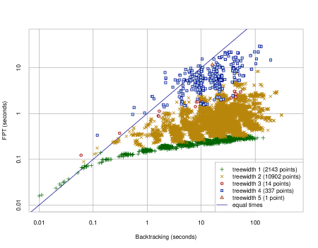
Figure 3: Running times for the 13 400 closed census manifolds

The second data set contains the first $500$ (much larger) triangulations from the Hodgson-Weeks census of closed hyperbolic manifolds [8]. This shows performance on larger triangulations, with $n$ ranging from $9$ to $20$.

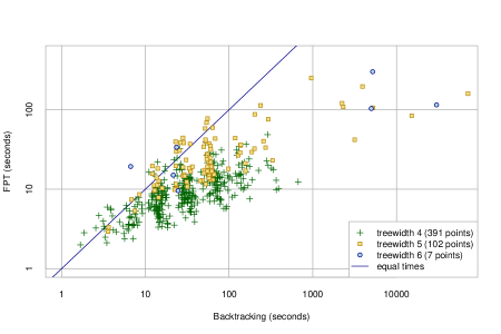
Figure 4: Running times for the first 500 Hodgson-Weeks census manifolds

Figures 3 and 4 compare the performance of both algorithms for each data set. All running times are for $\mathrm{TV}_{7,1}$ (the largest $r$ for which the experiments were feasible), and are measured on a single 3 GHz Intel Core i7 CPU. Both plots use a log-log scale with one data point per input triangulation. The results are striking: the FPT algorithm runs faster in over $99\%$ of cases, including most of the cases with largest treewidth. In the worst example the FPT algorithm runs $3.7\,\times$ slower than the backtracking, but both data sets have examples that run $>440\,\times$ faster. It is also pleasing to see a clear impact of the treewidth on the performance of the FPT algorithm, as one would expect.

6 An alternate geometric interpretation

In this section, we give a geometric interpretation of admissible colourings on a triangulation of a $3$-manifold $\mathfrak{T}$ in terms of normal arcs, i.e., straight lines in the interior of a triangle which are pairwise disjoint and meet the edges of a triangle, but not its vertices (see Figure 5). More precisely, we have the following

Theorem 7.

Given a $3$-manifold triangulation $\mathfrak{T}$, and $r\geq 3$, an admissible colouring of the edges of $\mathfrak{T}$ with $r-1$ colours corresponds to a system of normal arcs in the 2-skeleton with $\leq r-2$ arcs per triangle forming a collection of cycles on the boundary of each tetrahedron of $\mathfrak{T}$.

Proof.

Following the definition of an admissible colouring from Section 2.1, the colours of the edges $e_{1}$, $e_{2}$, $e_{3}$ of a triangle $f$ of $\mathfrak{T}$ must satisfy the parity condition, the triangle inequalities, and the upper bound constraint.

For a colouring $\theta(e)$ of an edge $e$, we define $\phi(e)=2\theta(e)$ which is an integer; we also use the term ”colouring” for $\phi$. We interpret the colourings $\phi(e_{1}),\phi(e_{2}),\phi(e_{3})\in\{0,1,\ldots,r-2\}$ as the number of intersections of normal arcs with the respective edges of the triangulation (see Figure 5). Without loss of generality, let $\phi(e_{1})\geq\phi(e_{2})\geq\phi(e_{3})$. We construct a system of normal arcs by first drawing $\phi(e_{2})$ arcs between edge $e_{1}$ and $e_{3}$ and $\phi(e_{1})-\phi(e_{2})$ arcs between edge $e_{1}$ and $e_{3}$. This is always possible since $\phi(e_{1})\leq\phi(e_{2})+\phi(e_{3})$ by the triangle inequality. Furthermore, the parity condition ensures that an even number of unmatched intersections remains which, by construction, all have to be on edge $e_{3}$. If this number is zero we are done. Otherwise we start replacing normal arcs between $e_{1}$ and $e_{2}$ by pairs of normal arcs, one between $e_{1}$ and $e_{3}$ and one between $e_{2}$ and $e_{3}$ (see Figure 5). In each step, the number of unmatched intersection points decreases by two. By the assumption $\phi(e_{2})\geq\phi(e_{3})$, this yields a system of normal arcs in $f$ which leaves no intersection on the boundary edges unmatched. This system of normal arcs is unique for each admissible triple of colours. By the upper bound constraint, we get at most $r-2$ normal arcs on $f$.

Looking at the boundary of a tetrahedron $t$ of $\mathfrak{T}$ these normal arcs form a collection of closed cycles. To see this, note that each intersection point of a normal arc in a triangle with an edge is part of exactly one normal arc in that triangle and that there are exactly two triangles sharing a given edge. ∎

Figure 5: Constructing a system of normal arcs from edge colourings.

Now, let $\mathfrak{T}$ be a closed $n$-tetrahedron $3$-manifold triangulation, $t$ a tetrahedron of $\mathfrak{T}$, $f_{1}$ and $f_{2}$ two triangles of $t$ with common edge $e$ of colour $\phi(e)$, and $a_{i}$ and $b_{i}$ the respective non-negative numbers of the two normal arc types in $f_{i}$ meeting $e$, $i\in\{1,2\}$. Since the system of normal arcs on $t$ forms a collection of cycles on the boundary of $t$, we must have $a_{1}+b_{1}=a_{2}+b_{2}\leq r-2$, giving rise to a total of $6n$ linear equations and $12n$ linear inequalities on $6n$ variables which all admissible colourings on $\mathfrak{T}$ must satisfy. Thus, finding admissible colourings on $\mathfrak{T}$ translates to the enumeration of integer lattice points within the polytope defined by the above equalities and inequalities.

Now, if we drop the upper bound constraint above, we get a cone. Computing the Hilbert basis of integer lattice points of this cone yields a finite description of all admissible colourings for any $r\geq 3$ and, thus, the essential information to compute $\mathrm{TV}_{r,q}(\mathfrak{T})$ for arbitrary $r$. Transforming this approach into a practical algorithm is work in progress.

7 Acknowledgement

This work is supported by the Australian Research Council (projects DP1094516, DP140104246).

References

- [1] Gorjan Alagic, Stephan P. Jordan, Robert König, and Ben W. Reichardt. Estimating Turaev-Viro three-manifold invariants is universal for quantum computation. Physical Review A, 82(4):040302(R), 2010.
- [2] Hans L. Bodlaender and Arie M. C. A. Koster. Treewidth computations. I. Upper bounds. Inform. and Comput., 208(3):259–275, 2010.
- [3] Benjamin A. Burton. Structures of small closed non-orientable 3-manifold triangulations. J. Knot Theory Ramifications, 16(5):545–574, 2007.
- [4] Benjamin A. Burton. Detecting genus in vertex links for the fast enumeration of 3-manifold triangulations. In ISSAC 2011: Proceedings of the 36th International Symposium on Symbolic and Algebraic Computation, pages 59–66. ACM, 2011.
- [5] Benjamin A. Burton, Ryan Budney, William Pettersson, et al. Regina: Software for 3-manifold topology and normal surface theory. http://regina.sourceforge.net/, 1999–2014.
- [6] Benjamin A. Burton and Rodney G. Downey. Courcelle’s theorem for triangulations. Preprint, arXiv:1403.2926, March 2014.
- [7] David G. Cantor and Erich Kaltofen. On fast multiplication of polynomials over arbitrary algebras. Acta Inf., 28(7):693–701, 1991.
- [8] Craig D. Hodgson and Jeffrey R. Weeks. Symmetries, isometries and length spectra of closed hyperbolic three-manifolds. Experiment. Math., 3(4):261–274, 1994.
- [9] Louis H. Kauffman and Sóstenes Lins. Computing Turaev-Viro invariants for -manifolds. Manuscripta Math., 72(1):81–94, 1991.
- [10] Robion Kirby and Paul Melvin. The -manifold invariants of Witten and Reshetikhin-Turaev for . Invent. Math., 105(3):473–545, 1991.
- [11] Robion Kirby and Paul Melvin. Local surgery formulas for quantum invariants and the Arf invariant. In Proceedings of the Casson Fest, volume 7 of Geom. Topol. Monogr., pages 213–233. Geom. Topol. Publ., Coventry, 2004.
- [12] Bruce Kleiner and John Lott. Notes on Perelman’s papers. Geom. Topol., 12(5):2587–2855, 2008.
- [13] T. Kloks. Treewidth: Computations and Approximations, volume 842. Springer, 1994.
- [14] Sergei Matveev. Algorithmic Topology and Classification of 3-Manifolds. Number 9 in Algorithms and Computation in Mathematics. Springer, Berlin, 2003.
- [15] Sergei Matveev et al. Manifold recognizer. http://www.matlas.math.csu.ru/?page=recognizer, accessed August 2012.
- [16] James R. Munkres. Elements of algebraic topology. Addison-Wesley, 1984.
- [17] Neil Robertson and P. D. Seymour. Graph minors. II. Algorithmic aspects of tree-width. J. Algorithms, 7(3):309–322, 1986.
- [18] Seinosuke Toda. PP is as hard as the polynomial-time hierarchy. SIAM J. Comput., 20(5):865–877, 1991.
- [19] Vladimir G. Turaev and Oleg Y. Viro. State sum invariants of -manifolds and quantum -symbols. Topology, 31(4):865–902, 1992.
- [20] Leslie G. Valiant. The complexity of computing the permanent. Theor. Comput. Sci., 8:189–201, 1979.
- [21] Thomas van Dijk, Jan-Pieter van den Heuvel, and Wouter Slob. Computing treewidth with LibTW. Available from www.treewidth.com, 2006.
- [22] Kevin Walker. On Witten’s 3-manifold invariants. http://canyon23.net/math/, 1991.