An introduction to some imperfections of CCD sensors

Abstract

CCD sensors do not deliver a perfect image of the light they receive. Beyond the well known linear image smearing due to diffusion of charges during their drift towards the pixel wells, non-linear effects are at play in these sensors. We now have ample evidence for both a flux-dependent and static image distortions, especially but not only, on deep-depleted CCDs. For large surveys relying on CCD sensors, these effects should now be taken into account when reducing data. We present here a summary of current results on sensor characterization and mitigation methods.

1 Introduction

The first workshop on “ Precision Astronomy with Fully Depleted CCDs” was held at Brookhaven National Laboratory in November 2013. Most of the contributions discussed sensor effects affecting astronomical measurements using CCDs. We will here mostly summarize the findings reported then, and for some aspects, reported since then in the literature. A second iteration of the same workshop took place in December 2014 in the same place. New results where presented there, and we refer interested readers to the program and proceedings.

CCD do not map the incoming light along a perfect rectilinear and periodic grid. The departures of CCD images from this ideal mapping can be broadly split into two classes: static effects that do not depend on the charge stored in the device, and dynamic effects that increase as charge accumulates in the device. A striking example of static distortions are the so-called tree rings which are visible as concentric variations of the sensor response to a uniform illumination. These variations mimic annual growth rings of trees, and qualify as static because the pattern scales with illumination. We will discuss shortly the source of these patterns which were observed only recently on deep-depleted devices. On the contrary, dynamic distortions in CCDs vary with illumination, and a typical example is the variation of the size of Point Spread Function (PSF, i.e. the response to point sources) with intensity. Although a sizable PSF variation was only recently observed (again on deep-depleted CCDs), there are much earlier reports of phenomena belonging to this class: for example a small PSF size variation was predicted more than 40 years ago in [1]. About 10 years ago, it was reported that the variance in flat-fields does not scale with their average [2], at odds with Poisson statistics. This can also be attributed to dynamic distortions.

The plan of this contribution goes as follows: We first discuss static distortions, then dynamic ones, and finally provide some outlook.

2 Static distortions

By definition static distortions are independent of the illumination level. For example a position dependent displacement of astronomical objects is a static distortion. A historical cause of static distortions of the images is due to a column or row having a physical size different from the average. This kind of defect might cause detectable astrometric shifts (see e.g [3], Appendix B of [4]) and is not specific to some kind of CCD. We do not know of such defects reported on recent CCDs (in particular the deep-depleted devices discussed at this workshop), perhaps because manufacturers have eliminated the causes. On the contrary, the defects we discuss in this section seem to be largely specific to deep-depleted CCDs, or at least they significantly increase with the device thickness.

2.1 Tree rings

The tree ring patterns of flat-field images are observed on most of the deep-depleted devices. They consist of concentric variations of the flat-field response to a uniform illumination. The center of the circles coincides with the center of the ingot from which the sensor was manufactured, as discussed in [5]. On DECam, these variations amount to about 0.2% (y band) to 0.4% (g band) peak to peak [6], and the patterns look alike in different bands. If the flat-field image (with these rings) is used to actually flat-field the science images, one observes photometry offsets spatially correlated with the flat-field variations [6]. This suggests that these flatfield variations do not originate from conversion efficiency inhomogenities but rather from pixel size variations. Indeed, applying to science images flatfield variations due to pixel size inhomogeneities degrades photometric uniformity. This hypothesis that the tree rings are due to pixel size variations is strongly supported by the spatial correlation of astrometry residuals and the gradient of flat-field variations [6].

The physical picture one can draw is the following: during the growth of the silicon boule, there are time-dependent variations of silicon purity, which translate into small static distortions of the drift field in the sensor[5, 6]. Those distortions in turn displace the image in a position-dependent way and the divergence of the displacement field is observed as pixel size variations imprinted on flat-field images. Since the tree rings have periods above tens of pixels, one can represent the displacement field as continuous. Calling $\overrightarrow{\delta}$ this displacement field, (i.e. the average shift in the image plane from the conversion point to the collection point), and expressing charge conservation, the observed flatfield image $F^{\prime}$ reads

$$F^{\prime}(\overrightarrow{x}+\overrightarrow{\delta})=F(\overrightarrow{x})\left|{\mathrm{d}et}\frac{\partial\overrightarrow{x}}{\partial(\overrightarrow{x}+\overrightarrow{\delta})}\right|=F(\overrightarrow{x})\left(1-div\overrightarrow{\delta}+o(\overrightarrow{\delta}^{2})\right)$$

where F is the illumination pattern at the conversion point. The stronger effect at bluer wavelengths is naturally attributed to their average longer drift path than red wavelengths (for back-illuminated CCDs), and hence larger transverse shifts. This displacement field ansatz (due to drift field distortions) also explains the size of the observed correlations of photometric and astrometric offsets with the flat-field pattern [6]. Incidentally, the quality of these correlations observed on DECam leaves little room (i.e. less that about one part in a thousand) for flat-field variations due to genuine variations of sensor efficiency, at least over spatial scales below $\sim$ 50 pixels.

2.2 Distorted drift fields on sensor edges

On a CCD device, one might expect distortions of the drift electric field at a distance from the sensor edges of the order of the sensor thickness. For thick devices, this can amount to more than ten pixels. Thick deep-depleted CCDs generically exhibit distortions of the flat-field on the sensor edges, either a flux deficit (a roll-off, e.g. [7]), or a flux increase (“glowing edges” on DECam, [6]), depending on the CCD type. We will generically call roll-off the effect in what follows, but what is discussed here applies as well to brighter edge stripes.

One can prove that this response roll-off is due to the electric field being not perpendicular to the sensor surface, again by relating astrometric displacements to the flatfield changes. This is done for the e2v LSST candidates in [7]. So, the response roll-off is another manifestation of a displacement field, as tree rings, and techniques to map tree rings will also capture these distortions on the sensor edges.

A possible handling of these defects consists of just ignoring the edges. One can note that tree rings call for a general framework to handle sensor-induced static astrometric distortions, which could handle as well the response roll-off on sensor edges, in order to salvage both astrometric and shape measurements. How much of the affected edge will be recovered remains unknown today.

The response roll-off on the edges causes spatial charge gradients in the image. The dynamic distortions we will discuss in next section tend to smear contrasts, more specifically to cause larger smearing to larger contrasts. As a consequence the shape of the roll-off does not exactly scale with illumination, as was observed on two LSST sensor candidates [8]. For science observations, this means that the handling of the edge roll-off should in principle depend on the sky background collected in the image. However, if one implements the correction of dynamic distortions at the pixel level (as suggested in [9, 10]), the dependence on the sky background of the response roll-off is accounted for in this correction. The bulk of the effect still remains to be corrected for, using some mapping of the displacement field.

2.3 Static distortions and flat fielding

When reducing CCD data, it is fairly common to divide every image by some average of flat-field frames in order to compensate for efficiency variations. When the spatial variations of flat-field are dominated by pixel size variations, this is likely to degrade the photometric uniformity [11]. Assuming the contribution of pixel size variations to the flat-field can be evaluated, one might be tempted to take those out of the flat-field. This would leave spatial variations of the sky background in science images which would make the sky subtraction inaccurate if not unpractical. So, over spatial scales smaller than the ones used for sky background evaluation, the pixel size variations have to be left into the flat-field frame and their effect on photometry should be corrected for in image catalogs.

3 Dynamic distortions

Dynamic distortions are characterized by departures from a linear response: the relation between the image and the illumination (slightly) depends on the illumination level, even well below the saturation level of the sensor, and independently of possible non-linearity of the electronic chain.

3.1 Fat PSF or the brighter-fatter effect

The growth of the PSF width with flux (e.g. [9]) is a striking example of dynamic response distortion. The increase in size reaches $\sim$ 2% from zero flux to saturation on one of LSST candidate sensors (the CCD 250 from e2v, 100 $\mu$ thick, 10$\mu$m pitch). The size increase is smaller ($\sim$ 1%) on the DECam sensors (LBNL CCDs, 250 $\mu$m thickness, 13.5 $\mu$m pitch). We do not know of any failed attempt to observe this effect, even on thinned CCDs ([4]), where is at only a few per mil level. We do not know either of any reported evidence of chromaticity of the effect. All reports are compatible with a slightly steeper increase (by $\sim$ 20 %) of the PSF size along the columns than along the rows. This phenomenon qualifies as non-linear because the response does not exactly scale with illumination.

A relative increase of 1% of the PSF size should be properly addressed for at least two scientific applications of astronomical imaging : precision PSF photometry of faint vs bright sources (necessary for example for measuring luminosity distances to supernovae), and cosmic shear measurements via galaxy ellipticities (which involve comparing the second moments of faint galaxies and brighter stars). Qualitatively, the brighter-fatter effect is a smearing of the image increasing with illumination, and the next section deals with another behavior that could be described using the same expression.

3.2 Departure from Poisson fluctuations in uniform exposures

The non-linearity of the Photon Transfer Curve (PTC) (e.g. [2]) is some other unexpected behavior of CCDs. Namely one observes that the spatial variance of uniform illuminations does not scale with their average, but slightly falls off, at odds with expectations from Poisson statistics. Unsurprisingly, this “variance deficit” comes with (mostly) positive correlations between nearby pixels which decay with spatial separation. These correlations also scale with the average illumination [2, 9, 12].

The fact that the variance does not scale exactly with the average qualifies indeed as non-linearity, as the following sketch shows. Let us split a uniform long illumination into smaller time chunks. If the device is perfectly linear, the various chunks are independent and both their averages and variances just add up when assembling the long exposure. So, a non-linear PTC indicates a response non-linearity, and one can suspect that because of causality, when integrating an image, the late stages of charge accumulation are influenced by the outcome of earlier stages.

So, the bending of the PTC is non-linear, and corresponds, as the brighter-fatter effect, to a smearing of the response, increasing with the exposure level. Since we observe that the statistical correlations, up to sensor saturation, grow as the average $\mu$ of the flatfield, we get that the covariance of pixels separated by $i$ rows and $j$ lines vary like $Cov_{ij}\propto\mu V$, where $V$ is the variance of the flatfield. In a charge-conserving process, this evolution of covariances comes with a compensating evolution of the variance (which is hence not exactly Poissonian), because the integral of the correlation function is conserved by charge redistribution (see e.g. the appendices of [2, 13]). In both [2, 13], it is also checked that summing the correlations actually restores the linearity of the PTC.

With $Cov_{ij}\propto\mu V$, i.e. $Cov_{ij}\propto\mu^{2}$ to first order of perturbations, one expects that the variance of uniform exposures is a quadratic function of their average, as observed (e.g. [2, 9, 13]). Note that the quadratic correction to Poisson statistics is not dominant: the variance deficit is typically of the order of 10 % at saturation. The correlations between nearest neighbors are in the percent range at saturation and rapidly decay to typically $10^{-4}$ at a few pixel separation.

3.3 Relating correlations and the brighter-fatter effect

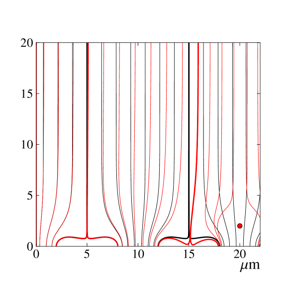
Figure 1: Electrostatic computation of field lines in a 100 $\mu$m thick, 10 $\mu$m pitch CCD. The clock lines are perpendicular to the picture plane, the picture only displays the 20 $\mu$m part that contains the clock stripes, and the buried channel has not been implemented in the setup . One set of field lines applies to the empty device, and the other applies to the device with 50 000 ke in one of the potential wells (red spot). In both instances, the thick field lines are the effective pixel boundaries. Note that adding this charge actually shrinks the pixel in which it resides, and also to a lesser extend its neighbors. Note that the effect of the distortions is concentrated in the last microns of the drift and hence essentially do not depend on the conversion point of the photons. The dynamic distortions are then mostly achromatic, as observed. This figure is borrowed from [13].

In [9] it is proposed that correlations in uniform exposures and the brighter-fatter effect share the same origin, namely the distortions of the electric field sourced by the charges stored in the potential wells of the sensor, as illustrated by an electrostatic computation in Fig. 1. This assumption is supported by crude electrostatic calculations, which show that adjusting the size of field distortions induced by some arbitrary charge, one can reproduce (to significantly better than a factor of 2) both the flatfield correlations and how rapidly spot widths increase with flux. Establishing how stored charges distort the field lines in the vicinity of the charge buckets requires a precise knowledge of the geometry and nature of the clock stripes and channel stops. This is usually not provided together with sensors, and some of this information is even regarded as proprietary by sensor vendors. It is thus tempting to derive how stored charges affect drift paths from measured correlations in uniform exposures, in order to infer the brighter-fatter effect. Note that this simple physical model of distortions also explains why the observed effects are mostly achromatic: stored charges affect the electric field mostly in the vicinity of the pixel wells (see Fig. 1), and hence affect all wavelengths equally. We might however expect some manifestations of chromaticity of correlations at large distances. The reduction of the drift electric field by charges stored in the potential wells increases lateral diffusion (see e.g. [14] and references therein), and this increase is generally a small contribution to the brighter-fatter effect [13], but it is chromatic as well.

If the brighter-fatter effect manifests itself as a mostly linear increase of the PSF as a function of flux (or peak flux), one cannot exclude that the effect is more than just a scaling of size. Identifying the physical mechanism that causes this apparent increase is the way to safely model the average evolution of the shape of point-like objects as a function of their flux. Once this is done, bright stars can safely be used to e.g. unfold the finite PSF size from measurements of faint galaxy shapes, as required by cosmic shear measurements.

Ref. [9] proposes a first order empirical parametrization of pixel boundary shifts induced by stored charges. This simple model describes the correlations in uniform exposures linearly rising with the average content, the quadratic behavior of the PTC, and the essentially linear rise of the PSF size with peak flux. The critical test of the model (in fact of any model relating correlations and the brighter-fatter effect) consists in extracting the model parameters from flat-fields, and then quantitatively compare the predicted PSF width evolution with flux with the measured one.

The model proposed in [9] has about twice more parameters than available correlations to measure. Ref. [9], [13], and [10] follow similar strategies in order to overcome this limitation: they assume that the electrostatic forces sourced by stored charges decay smoothly with distance. The details of how smoothness is imposed do not seem to alter significantly the result. These three works provide evidence that the brighter-fatter slope can be predicted from correlations in uniform exposures. Ref. [13] find a 5% mismatch compatible with the statistics in use.

4 Further work and outlook

We seem to have now physical explanations for both static and dynamic distortions: the former are due to the drift electric field (in the bulk of the device) not being orthogonal to the surface, either because of inhomogeneities of the bulk properties, or to the electric field being distorted on the edges. The dynamic distortions are due to the electric field being affected by the charges stored in the potential wells. Because the dynamic distortions mostly happen near the charge buckets, and the static ones along the whole drift path, static distortions are chromatic while the dynamic ones are mostly achromatic. Note that although the edge roll-off is both static and dynamic, the separation we are proposing remains pertinent.

Static distortions are important to map out because they affect both flux and shape measurements. A detailed study of the static distortions in DECam is presented in [6] and proposes a simple recipe to handle the tree rings: it determines the displacement field from flat-field inhomogenities, assuming that these perturbations are entirely due to displacements, and that displacements follow a radial pattern. This last conditions allows one to turn a scalar field (the flatfield inhomogenities) into a 2-d vector displacement field in the image plane. Whether this simple method can be applied in general is questionable, and a practical method to separate quantum efficiency variations from a displacement field is still to be demonstrated. Since the 2-d displacements are due to transverse drift fields, one can argue that this 2-d displacement field has a null rotational, which turns it back into a scalar field. However, one would probably keep this property for a sanity check rather than reducing the solution space to fields deriving from a potential. Incidentally, cosmic shear fields (which are as well irrotational) are usually not evaluated under this constraint (see e.g. [15]), but it is rather used as a check.

In order to separate pixel size effects for genuine sensor efficiency variations, we do not know of a simple method so far. We can think of two avenues. In the laboratory, one can illuminate devices with spatially varying patterns, and with enough rotations and shifts of the same pattern, one can solve for the displacement field, sensor efficiency, and, if needed, the illumination pattern itself. Several enterprises along these lines are being developed but the proof of concept is still to be delivered. On the sky, one can measure the displacement field from astrometry (e.g. [6]), evaluate the effect on flat-fields and attribute what is left in flat fields to sensor efficiency variations. Reasonably, projects now assembling their hardware (like LSST) should follow both avenues.

Reference [10] constitutes arguably the first large scale attempt to infer the brighter-fatter effect from pixel correlations, and the results are encouraging. One might then regard electrostatic modelling as a useless complication, especially since this work detects correlations slopes that change from sensor to sensor, which are difficult to reduce to variation between sensor batches. In our opinion, it is still pertinent to develop full realistic electrostatic models, because we cannot exclude that the sensor parameters required for these simulations might be constrained from measurements of correlations. Furthermore, since we expect that some level of chromatism of correlations is eventually detected, this might further constrain the simulated electrostatic configurations.

- [1] W. H. Kent, Charge distribution in buried-channel charge-coupled devices, The Bell System Technical Journal 52 (Jan., 1973).
- [2] M. Downing, B. Baade, P. Sinclaire, S. Deiries, and F. Christen, CCD riddle: a) signal vs time: linear; b) signal vs variance: non-linear, Proc SPIE (2006) 6276–09.
- [3] J. Anderson and I. R. King, Astrometric and Photometric Corrections for the 34th Row Error in HST’s WFPC2 Camera, PASP 111 (Sept., 1999) 1095–1098.
- [4] P. Astier, P. El Hage, J. Guy, D. Hardin, M. Betoule, S. Fabbro, N. Fourmanoit, R. Pain, and N. Regnault, Photometry of supernovae in an image series: methods and application to the SuperNova Legacy Survey (SNLS), A&A 557 (Sept., 2013) A55, [\hrefhttp://xxx.lanl.gov/abs/1306.5153arXiv:1306.5153].
- [5] L. Altmannshofer, M. Grundner, J. Virbulis, and J. Hage, A material innovation for the electronic industry: float zone single crystal silicon with 200mm diameter, in Power Semiconductor Devices and ICs, 2003. Proceedings. ISPSD ’03. 2003 IEEE 15th International Symposium on, pp. 325–328, April, 2003.
- [6] A. A. Plazas, G. M. Bernstein, and E. S. Sheldon, Transverse electric fields’ effects in the dark energy camera ccds, Journal of Instrumentation 9 (2014), no. 04 C04001.
- [7] P. O’Connor, Spot scan probe of lateral field effects in a thick fully-depleted ccd, Journal of Instrumentation 9 (2014), no. 03 C03033.
- [8] A. Guyonnet and A. Tyson. Private communications, 2014.
- [9] P. Antilogus, P. Astier, P. Doherty, A. Guyonnet, and N. Regnault, The brighter-fatter effect and pixel correlations in CCD sensors, Journal of Instrumentation 9 (Mar., 2014) C3048, [\hrefhttp://xxx.lanl.gov/abs/1402.0725arXiv:1402.0725].
- [10] D. Gruen, G. M. Bernstein, M. Jarvis, B. Rowe, V. Vikram, A. A. Plazas, and S. Seitz, Characterization and correction of charge-induced pixel shifts in DECam, ArXiv e-prints (Jan., 2015) [\hrefhttp://xxx.lanl.gov/abs/1501.0280arXiv:1501.0280].
- [11] C. W. Stubbs, Precision astronomy with imperfect fully depleted CCDs - an introduction and a suggested lexicon, Journal of Instrumentation 9 (Mar., 2014) C3032, [\hrefhttp://xxx.lanl.gov/abs/1312.2313arXiv:1312.2313].
- [12] R. H. Lupton, Consequences of thick ccds on image processing, Journal of Instrumentation 9 (2014), no. 04 C04023.
- [13] A. Guyonnet, P. Astier, P. Antilogus, N. Regnault, and P. Doherty, Evidence for self-interaction of charge distribution in charge-coupled devices, A&A, in press (2015).
- [14] S. E. Holland, C. J. Bebek, W. F. Kolbe, and J. S. Lee, Physics of fully depleted ccds, Journal of Instrumentation 9 (2014), no. 03 C03057.
- [15] L. Fu, E. Semboloni, H. Hoekstra, M. Kilbinger, L. van Waerbeke, I. Tereno, Y. Mellier, C. Heymans, J. Coupon, K. Benabed, J. Benjamin, E. Bertin, O. Doré, M. J. Hudson, O. Ilbert, R. Maoli, C. Marmo, H. J. McCracken, and B. Ménard, Very weak lensing in the CFHTLS wide: cosmology from cosmic shear in the linear regime, A&A 479 (Feb., 2008) 9–25, [\hrefhttp://xxx.lanl.gov/abs/0712.0884arXiv:0712.0884].