Hypergeometric analytic continuation of the strong-coupling perturbation series for the 2d Bose-Hubbard model

Abstract

We develop a scheme for analytic continuation of the strong-coupling perturbation series of the pure Bose-Hubbard model beyond the Mott insulator-to-superfluid transition at zero temperature, based on hypergeometric functions and their generalizations. We then apply this scheme for computing the critical exponent of the order parameter of this quantum phase transition for the two-dimensional case, which falls into the universality class of the three-dimensional $XY$ model. This leads to a nontrivial test of the universality hypothesis.

I Introduction

In many branches of theoretical physics one encounters the necessity to reconstruct an observable from a diverging perturbation series. This is possible because a divergent series, by itself, is not a bad thing, but still carries profound mathematical meaning Euler60 ; Hardy49 . Take, for example, the geometric series

$$\frac{1}{1-z}=\sum_{n=0}^{\infty}z^{n}\;,$$ (1)

where the sum on the right-hand side (r.h.s.) converges only for $|z|<1$. Nonetheless, if one regards the left-hand side (l.h.s.) as a definition of the formal sum, as already done by Euler Euler60 , that sum obtains a well-defined meaning even for $|z|>1$, giving, for instance, $1+2+4+8+\ldots=-1$. Similarly, quantum-mechanical perturbation theory may yield a formal series

$$A(\lambda)\sim\sum_{n=0}^{\infty}\alpha_{n}\lambda^{n}$$ (2)

for some quantity $A(\lambda)$, where $\lambda$ is a small parameter. The coefficients $\alpha_{n}$ may be such that the series is asymptotic, having zero radius of convergence, as it happens, e.g., when computing the ground-state energy of an anharmonic oscillator with a quartic perturbation of a quadratic potential BenderWu69 . The task then again is to identify the unknown true observable on the l.h.s. from the given formal sum on the r.h.s.

The concept that naturally comes into play here is analytic continuation. Still, for applying this concept in practice, when merely a few leading coefficients $\alpha_{n}$ are available, one needs to invoke some sort of a priori hypothesis about $A(\lambda)$, either explicitly or implicitly. For instance, if one possesses explicit knowledge of $A(\lambda)$ for large values of $\lambda$, one can exploit this for designing rapidly converging strong-coupling expansions from divergent weak-coupling perturbation series JankeKleinert95 ; KleinertEtAl97 ; JaschKleinert01 . When resorting instead to the more familiar Padé approximation technique BakerMorris96 ; CalicetiEtAl07 , one introduces rational approximants of the form

$$A_{L/M}(\lambda)=\frac{\sum_{n=0}^{L}p_{n}\lambda^{n}}{1+\sum_{n=1}^{M}q_{n}\lambda^{n}}$$ (3)

and equates the coefficients obtained from a Taylor series expansion of $A_{L/M}$ up to the order ${\mathcal{O}}(\lambda^{M+N})$ to those of the perturbation series (2). While the resulting Padé table then may yield good numerical values of the desired quantity, one is implictly imposing the asymptotic behavior $A_{L/M}(\lambda)\sim p_{L}\lambda^{L-M}/q_{M}$ for large $\lambda$, which may not be physically correct.

Recently, Mera, Pedersen, and Nikolić MeraEtAl14 have suggested to replace the rational Padé approximants (3) by hypergeometric functions, which represent another form of an implicit a priori hypothesis. The examples from elementary single-particle quantum mechanics studied by these authors suggest that the corresponding analytic continuation technique can dramatically outperform Padé and Borel-Padé approaches. Hence, it was conjectured that the hypergeometric-function scheme might also be useful for many-body problems of condensed-matter physicsMeraEtAl14 .

In the present letter we provide first evidence which strongly supports this conjecture. We consider the two-dimensional (2d) Bose-Hubbard model on a square lattice, which constitutes a system of paradigmatic importance for quantum many-body theory FisherEtAl89 ; FreericksMonien96 ; CapogrossoEtAl08 ; SantosPelster09 ; FreericksEtAl09 , and develop a “hypergeometric” technique for obtaining the critical exponents of its Mott insulator-to-superfluid transition.

We proceed as follows: We first briefly introduce the Bose-Hubbard model, and the strong-coupling perturbation series derived from it, which serves as input for the subsequent analysis. Next, we show how Gaussian hypergeometric functions ${}_{2}F_{1}$, and their generalizations ${}_{q+1}F_{q}$, emerge quite naturally when studying the quantum phase transition. We then apply our scheme for computing the phase diagram and the critical exponent of the order parameter. This is of some conceptual interest, since these exponents are supposed to be universal, but there is still a slight discrepancy Vicari07 between experimentally measured LipaEtAl03 and theoretically calculated CampostriniEtAl01 values. Our scheme opens up a fresh approach to this subtle issue.

II The model

We consider the pure Bose-Hubbard model for interacting Bose particles FisherEtAl89 ; FreericksMonien96 ; CapogrossoEtAl08 ; SantosPelster09 ; FreericksEtAl09 on a two-dimensional square lattice at zero temperature. In its grand-canonical version this model is characterized by three parameters: The hopping matrix element $J$, which quantifies the strength of the tunneling contact between neighboring lattice sites, the repulsion energy $U$ provided by each pair of particles occupying the same lattice site, and the chemical potential $\mu$. For a given value of $\mu$ the competition between particle delocalization due to tunneling and localization caused by repulsion leads to the well-known quantum phase transition from a Mott insulator to a superfluid when the ratio $J/U$ is gradually increased, starting from zero FisherEtAl89 . We employ the Fock-space operators $\hat{b}^{\dagger}_{i}$ and $\hat{b}^{\phantom{{\dagger}}}_{i}$ which create or annihilate a Boson at the $i$th site, so that

$$\hat{n}^{\phantom{{\dagger}}}_{i}=\hat{b}^{\dagger}_{i}\hat{b}^{\phantom{{\dagger}}}_{i}$$ (4)

counts the number of particles at that site, and use $U$ as the energy scale of reference. The non-dimensionalized Hamiltonian then is written as

$$\hat{H}_{\text{BH}}=\hat{H}_{0}+\hat{H}_{\text{tun}}\;,$$ (5)

where the site-diagonal part

$$\hat{H}_{0}=\frac{1}{2}\sum_{i}\hat{n}^{\phantom{{\dagger}}}_{i}(\hat{n}^{\phantom{{\dagger}}}_{i}-1)-{\mu}\big{/}{U}\sum_{i}\hat{n}^{\phantom{{\dagger}}}_{i}$$ (6)

models the on-site repulsion and incorporates the chemical potential to fix the particle number; this operator (6) serves as the starting point for perturbative expansions FreericksMonien96 . The further term

$$\hat{H}_{\text{tun}}=-{J}\big{/}{U}\sum_{\langle i,j\rangle}\hat{b}^{\dagger}_{i}\hat{b}^{\phantom{{\dagger}}}_{j}$$ (7)

accounts for the tunneling effect, with the sum ranging over all pairs of neighboring sites $i$ and $j$. Following Ref. SantosPelster09 , we then break the particle-number conservation implied by this Bose-Hubbard model (5) by adding spatially uniform sources and drains,

$$\hat{H}=\hat{H}_{\text{BH}}+\sum_{i}\eta(\hat{b}^{\dagger}_{i}+\hat{b}^{\phantom{{\dagger}}}_{i})\;,$$ (8)

where, without loss of generality, we have taken the dimensionless source strength $\eta$ to be real. The quantity of interest now is the intensive ground-state energy

$${\mathcal{E}}\!\left({J}\big{/}{U},{\mu}\big{/}{U},\eta\right)=\langle\hat{H}\rangle/M\;,$$ (9)

where the expectation value is taken with respect to the ground state of the extended model (8), and $M$ denotes the number of sites, assumed to be so large that finite-size effects do not matter. From this we obtain the susceptibility

$$2\psi=\frac{\partial{\mathcal{E}}}{\partial\eta}=2\langle\hat{b}^{\phantom{{\dagger}}}_{i}\rangle\;,$$ (10)

where the first identity constitutes the definition of $\psi$, and the second is provided by the Hellmann-Feynman theorem. When taken at $\eta=0$, this derivative describes the response of the original Bose-Hubbard model (5) to the sources and drains: The expectation value $\langle\hat{b}^{\phantom{{\dagger}}}_{i}\rangle=\psi$ is zero in the Mott-insulating phase, but takes on nonzero values in the superfluid phase, and thus serves as order parameter.

Assuming now that the ground-state energy per site can be expanded in a power series of $\eta$, we write

$${\mathcal{E}}\!\left({J}\big{/}{U},{\mu}\big{/}{U},\eta\right)\\ =e_{0}\!\left({J}\big{/}{U},{\mu}\big{/}{U}\right)+\sum_{k=1}^{\infty}c_{2k}\!\left({J}\big{/}{U},{\mu}\big{/}{U}\right)\eta^{2k}\;.$$ (11)

For each ${\mu}\big{/}{U}$ the coefficients $c_{2k}$, known as $k$-particle correlation functions, are then expanded in powers of ${J}\big{/}{U}$:

$$c_{2k}\!\left({J}\big{/}{U},{\mu}\big{/}{U}\right)=\sum_{\nu=0}^{\infty}\alpha_{2k}^{(\nu)}\!\left({\mu}\big{/}{U}\right)\left({J}\big{/}{U}\right)^{\nu}\;.$$ (12)

In order to make contact with the Landau theory of phase transitions Landau37 ; Landau69 ; LaLifV , the key idea now is to employ $\psi$ instead of $\eta$ as independent variable. This is achieved by means of a Legendre transformation, which leads to the effective potential SantosPelster09 ; BradlynEtAl09

$$\Gamma = {\mathcal{E}}-2\psi\eta$$ (13)

$$= e_{0}+a_{2}\psi^{2}+a_{4}\psi^{4}+a_{6}\psi^{6}+\mathcal{O}(\psi^{8})$$

with the one-particle-irreducible vertices

$$a_{2}=-\frac{1}{c_{2}}\;,\;a_{4}=\frac{c_{4}}{c_{2}^{4}}\;,\;a_{6}=\frac{c_{6}}{c_{2}^{6}}-\frac{4c_{4}^{2}}{c_{2}^{7}}\;,$$ (14)

having suppressed their dependence on $J/U$ and $\mu/U$. Since $\eta$ and $\psi$ constitute a Legendre-conjugated pair, this construction implies

$$\frac{\partial\Gamma}{\partial\psi}=-2\eta\;,$$ (15)

leading to the physical interpretation of the formalism: Since the actual Bose-Hubbard system (5) is recovered by setting $\eta=0$, the physical solutions correspond to the stable stationary points of $\Gamma$ SantosPelster09 ; BradlynEtAl09 .

Now one can invoke a standard argument: Assuming $a_{4}$ and $a_{6}$ to be positive, and neglecting higher order terms of the expansion (13), a single minimum of $\Gamma$ is found at $\psi_{\min}=0$ as long as $a_{2}>0$, indicating the Mott insulator phase. In contrast, if $a_{2}<0$ the minimum is found at $\psi_{\min}\neq 0$, thus signaling the presence of the superfluid phase. Therefore, for given chemical potential $\mu/U$ the transition occurs when $a_{2}=-1/c_{2}=0$, that is, at that value $(J/U)_{\rm c}$ at which the series

$$c_{2}\!\left({J}\big{/}{U},{\mu}\big{/}{U}\right)=\sum_{\nu=0}^{\infty}\alpha_{2}^{(\nu)}\!\left({\mu}\big{/}{U}\right)\,\left({J}\big{/}{U}\right)^{\nu}$$ (16)

starts to diverge TeichmannEtAl09a ; TeichmannEtAl09b . Moreover, from the usual Landau form $\Gamma\approx e_{0}+a_{2}\psi^{2}+a_{4}\psi^{4}$ one obtains

$$\psi_{\rm min}^{2}=\frac{-a_{2}}{2a_{4}}$$ (17)

for $J/U>(J/U)_{\rm c}$. Assuming $a_{4}$ to be positive and smooth at the transition, the exponent $\beta$ which characterizes the emergence of the order parameter according to

$$\psi_{\rm min}^{2}\sim\left[J/U-(J/U)_{\rm c}\right]^{2\beta}$$ (18)

is thus solely determined by $a_{2}=-1/c_{2}$. This sets the stage for the present work: Its starting point is the perturbation series (16) for the coefficient $c_{2}$. Although this series requires a small parameter $J/U$ it is referred to as a strong-coupling expansion FreericksMonien96 , since it should converge in the strongly correlated Mott regime. We have evaluated its coefficients $\alpha_{2}^{(\nu)}$ numerically up to the order $\nu_{\rm max}=10$ in $J/U$ TeichmannEtAl09a ; TeichmannEtAl09b ; HinrichsEtAl13 , making use of the process-chain approach as devised in general form by Eckardt Eckardt09 . This technique, which has been recognized as an extremely powerful method HeilVonderLinden12 , is based on Kato’s non-recursive formulation of the Rayleigh-Schrödinger perturbation series Messiah99 . Here we take these coefficients as input for determining optimal hypergeometric approximants to the Landau parameter $a_{2}$, as detailed in the following section, from which the respective exponents $\beta$ can then be read off directly.

III The Method

Given the coefficients $\alpha_{2}^{(\nu)}({\mu}\big{/}{U})$ for $\nu=0$, $1$, $2$, …, $\nu_{\rm max}$, the first task is to deduce the radius of convergence of the series (16). This can be accomplished only if some a priori knowledge concerning the unknown higher-order coefficients is invested. To this end, useful guidance is provided by the case of high dimensionality $d$: As explained in Ref. TeichmannEtAl09b , for $d\to\infty$ the expansion (16) becomes a geometric series,

$$c_{2}=\alpha_{2}^{(0)}\sum_{\nu=0}^{\infty}\left(-2d\,\alpha_{2}^{(0)}\right)^{\nu}\left({J}\big{/}{U}\right)^{\nu}\;,$$ (19)

from which one can immediately read off its radius of convergence

$$(J/U)_{\rm c}=\frac{-1}{2d\,\alpha_{2}^{(0)}}\;;$$ (20)

after working out $\alpha_{2}^{(0)}$, this leads precisely to the mean-field phase boundary FisherEtAl89 ; TeichmannEtAl09b

$$(J/U)_{\rm c}=\frac{({\mu}\big{/}{U}+1-g)(g-{\mu}\big{/}{U})}{2d\,({\mu}\big{/}{U}+1)}\;,$$ (21)

where the integer filling factor $g$ satisfies ${\mu}\big{/}{U}+1\geq g\geq{\mu}\big{/}{U}$. Consequently, in this limiting case the Landau coefficient $a_{2}=-1/c_{2}$ takes the simple form

$$a_{2}=\frac{-1}{\alpha_{2}^{(0)}}\left(1-\frac{J/U}{(J/U)_{\rm c}}\right)\;,$$ (22)

exhibiting the mean-field exponent $2\beta=1$.

Figure 1: Ratios ${\alpha_{2}^{(\nu)}}\big{/}{\alpha_{2}^{(\nu-1)}}$ of subsequent coefficients of the series (16) for $d=2$ and ${\mu}\big{/}{U}=0.3769$, as corresponding to the tip of the lowest Mott lobe shown in Fig. 3. The solid horizontal line indicates the limit $1/(J/U)_{\rm c}^{\rm QMC}=1/0.05974(3)$ expected from QMC calculations CapogrossoEtAl08 . Observe that all coefficients $\alpha_{2}^{(\nu)}$ have the same sign, which impedes the Borel summability of the series (16).

For finite dimension $d$, however, the ratio ${\alpha_{2}^{(\nu)}}\big{/}{\alpha_{2}^{(\nu-1)}}$ of subsequent coefficients is not constant. For $d=2$ this is shown exemplarily in Fig. 1 for $\mu/U=0.3769$, corresponding to the tip of the lowest Mott lobe of the phase diagram depicted later in Fig. 3. Thus, the corresponding series (16) is no longer geometric, so that it is tempting to assume a Landau coefficient of the form

$$a_{2}=\frac{-1}{\alpha_{2}^{(0)}}\left(1-\frac{J/U}{(J/U)_{\rm c}}\right)^{2\beta}\;,$$ (23)

thereby admitting nontrivial exponents $2\beta$. According to this educated guess, the expansion (16) should have the form of a binomial series,

$$c_{2}=\alpha_{2}^{(0)}\sum_{\nu=0}^{\infty}\frac{(2\beta)_{\nu}}{\nu!}\left(\frac{J/U}{(J/U)_{\rm c}}\right)^{\nu}\;,$$ (24)

where $(a)_{\nu}=a(a+1)\cdots(a+\nu-1)$ is the usual Pochhammer symbol AbramowitzStegun72 . From an optimal fit of the given coefficients $\alpha_{2}^{(\nu)}$ to this hypothesis one could then determine approximate values of the two parameters $2\beta$ and $(J/U)_{\rm c}$.

But this guess can still be improved: Realizing that the binomial series coincides with the function ${}_{1}F_{0}$, employing the nomenclature used for generalized hypergeometric functions EMOT55 , one may generalize the a priori ansatz (24) further and require

$$c_{2} = \alpha_{2}^{(0)}{{}_{2}F_{1}}\!\left(a,b;c;\frac{J/U}{(J/U)_{\rm c}}\right)$$ (25)

$$= \alpha_{2}^{(0)}\sum_{\nu=0}^{\infty}\frac{(a)_{\nu}\,(b)_{\nu}}{\nu!\,(c)_{\nu}}\left(\frac{J/U}{(J/U)_{\rm c}}\right)^{\nu},$$

where now ${}_{2}F_{1}(a,b;c;z)$ denotes the well-known Gaussian hypergeometric function AbramowitzStegun72 ; EMOT55 , giving us four degrees of freedom for a least-square fit to the $\nu_{\rm max}$ perturbative data. The strength of its singularity at the point of divergence is given by

$${{}_{2}F_{1}}(a,b;c;z)\propto\frac{1}{(1-z)^{a+b-c}}\qquad\text{for }z\to 1\;,$$ (26)

from which one finds the exponents

$$2\beta=a+b-c\;.$$ (27)

Going still one step further, one may replace ${}_{2}F_{1}$ by a generalized hypergeometric function ${}_{q+1}F_{q}$ providing $2q+2$ degrees of freedom, requiring the evaluation of the perturbation series at least to the corresponding order. This possibility to perform analytic continuation of a perturbation series by means of an analytic function which itself is a member of a general familiy of “higher order” functions is the core of the proposal made in Ref. MeraEtAl14 . The hypergeometric functions, just as the binomial series, can adopt complex values beyond their radius of convergence. In view of its physical meaning we require $c_{2}$, as well as $a_{2}$, to be a real quantity, so that we take the real part of ${{}_{q+1}F_{q}}$. Technically, this is achieved by computing $\lim_{\varepsilon\to 0}\big{(}{{}_{q+1}F_{q}}(x+{\rm i}\varepsilon)+{{}_{q+1}F_{q}}(x-{\rm i}\varepsilon)\big{)}/2$.

Thus, from the expectation of a nontrivial exponent we infer that $c_{2}$ has to have an essential singularity at $(J/U)_{\rm c}$ with a strength determining the respective exponent. This is why ${}_{q+1}F_{q}$ are suitable approximants: As exemplified by Eq. (26), the strength of their singularities can be tuned by adjusting their parameters.

IV Results

We have applied this strategy to the series (16) for the two-dimensional Bose-Hubbard model with $0\leq\mu/U\leq 4$, having at disposal its coefficients $\alpha_{2}^{(\nu)}$ up to $\nu_{\max}=10$ TeichmannEtAl09a ; TeichmannEtAl09b ; HinrichsEtAl13 . Figure 2 again displays the ratios ${\alpha_{2}^{(\nu)}}\big{/}{\alpha_{2}^{(\nu-1)}}$ of subsequent coefficients for $\mu/U=0.3769$, now plotted vs. the reciprocal order $1/\nu$. In addition, we also indicate by continuous lines the ratios resulting from the best fit

$$\alpha_{2}^{(\nu)}=\alpha_{2}^{(0)}\cdot\frac{\big{(}1.405\big{)}_{\nu}}{\nu!}\cdot 16.51^{\nu}$$ (28)

to the binomial series hypothesis (24), and from the best fit

$$\alpha_{2}^{(\nu)}=\alpha_{2}^{(0)}\cdot\frac{\big{(}1.398\big{)}_{\nu}\,\big{(}-0.7684\big{)}_{\nu}}{\nu!\,\big{(}-0.7606\big{)}_{\nu}}\cdot 16.61^{\nu}$$ (29)

to the Gaussian hypergeometric hypothesis (25). Evidently, the quality of these fits is excellent. This allows us to perform reliable extrapolations to $\nu\to\infty$, where the ratios should approach the expected value $1/(J/U)_{\rm c}^{\rm QMC}=1/0.05974(3)$ known from quantum Monte Carlo (QMC) simulations CapogrossoEtAl08 . In addition, we have also fitted the exact coefficients to those of generalized hypergeometric functions ${}_{3}F_{2}$ and ${}_{4}F_{3}$.

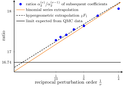
Figure 2: Ratios ${\alpha_{2}^{(\nu)}}\big{/}{\alpha_{2}^{(\nu-1)}}$ of subsequent coefficients of the series (16) for $d=2$ and $\mu/U=0.3769$, plotted vs. the reciprocal order $1/\nu$, together with the corresponding ratios obtained from the fit (28) to the binomial series, and from the fit (29) to the Gaussian hypergeometric function. Again, the horizontal line indicates the limit $1/(J/U)_{\rm c}^{\rm QMC}=1/0.05974(3)$ expected from QMC calculations CapogrossoEtAl08 .

Performing these procedures for all values of the chemical potential that are of interest, and reading off the respective values of $(J/U)_{\rm c}$, we obtain the system’s phase diagram. In Fig. 3 we show this diagram for $0\leq\mu/U\leq 4$, as resulting from the binomial and from the Gaussian hypergeometric fit, respectively. The relative deviation between both curves stays below 4%. It is largest halfway between the position of a tip of a Mott lobe and the nearest integer values of $\mu/U$; at the tips these deviations are smaller than $1\%$.

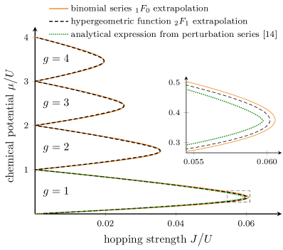
Figure 3: Zero-temperature phase diagram of the 2d Bose-Hubbard model as obtained from the binomial series hypothesis, and from the Gaussian hypergeometric hypothesis. Inside the lobes the system is in a Mott insulator state with $g$ particles per site, outside these lobes in a superfluid state. Also shown is the expression for the lowest Mott lobe stated in Ref. FreericksEtAl09 .

The tips of the Mott lobes represent multicritical points with particle-hole symmetry; here the system falls into the universality class of the $(d+1)$-dimensional $XY$ model FisherEtAl89 . The critical scaled hopping strength $(J/U)_{\rm c}$ at the tip of the lowest lobe for $d=2$, as provided by the respective fit, figures as

$${{}_{1}F_{0}} \;:\;(J/U)_{\rm c}\;=\;0.06056$$ (30)

$${{}_{2}F_{1}} \;:\;(J/U)_{\rm c}\;=\;0.06021$$

$${{}_{3}F_{2}} \;:\;(J/U)_{\rm c}\;=\;0.06003$$

$${{}_{4}F_{3}} \;:\;(J/U)_{\rm c}\;=\;0.06004\;,$$

which matches the QMC value $(J/U)_{\rm c}^{\rm QMC}=0.05974(3)$ quite well. If we assume this value to be exact, and take the result provided by ${}_{2}F_{1}$ as sound compromise between the number of coefficients available and the number of fit parameters, the error of that result is less than $1\%$.

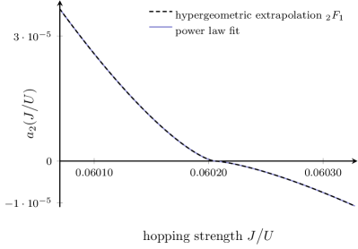
Figure 4: Behavior of the Landau coefficient $a_{2}$ for $\mu/U=0.3769$, as obtained by Gaussian hypergeometric continuation; for $J/U>(J/U)_{\rm c}$ the real part is shown. Also shown is the power-law fit (31).

So far, we have used hypergeometric continuation merely to reproduce existing knowledge, thus confirming its reliability. However, with the determinantion of the order parameter’s exponent we now move to a ground which is technically far more demanding RanconDupuis11 . In Fig. 4 we show the Gaussian hypergeometric description of the Landau coefficient $a_{2}$, and its analytic continuation beyond the transition point, again at the tip of the lowest Mott lobe. The data are well described by the power-law fit

$$8.679\big{(}(J/U)_{\rm c}-J/U\big{)}^{1.390} J/U<(J/U)_{\rm c}$$ for (31)

$$-2.945\big{(}J/U-(J/U)_{\rm c}\big{)}^{1.390} J/U>(J/U)_{\rm c}.$$ for

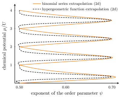
Figure 5: Exponents $\beta$ of the order parameter $\psi$ for the Mott insulator-to-superfluid transition, as obtained by binomial and Gaussian hypergeometric continuation, respectively. The “critical” value $\beta_{c}\approx 0.69$ is adopted at the tips of the Mott lobes.

Performing this procedure within the interval $0\leq\mu/U\leq 4.0$ for both the binomial and the Gaussian hypergeometric ansatz, we obtain the exponents displayed in Fig. 5. While both variants lead to notably different results for general $\mu/U$, they agree quite well at the tip of the lobes, i.e., at the critical points. This observation is quite significant, since one expects nontrivial critical exponents only at the tips of the lobes, while the system should be mean-field like for all other ${\mu}\big{/}{U}$. Our approximate scheme can only yield continuous lines, and it is an open question whether these would reduce to $\delta$-like spikes with higher orders. However, the relative stability of the data at the lobes’ tips indicates that one can actually determine the true critical exponent $\beta_{\rm c}$ of the Mott insulator-to-superfluid transition with good accuracy by hypergeometric continuation. In particular, at the tip of the lowest lobe we obtain the following values:

$${{}_{1}F_{0}} \;:\;\beta_{\rm c}\;=\;0.7023$$ (32)

$${{}_{2}F_{1}} \;:\;\beta_{\rm c}\;=\;0.6949$$

$${{}_{3}F_{2}} \;:\;\beta_{\rm c}\;=\;0.6881$$

$${{}_{4}F_{3}} \;:\;\beta_{\rm c}\;=\;0.6904\;.$$

This gives rise to a nontrivial test of the universality hypothesis for critical phenomena. Using the scaling relation $\beta_{c}=(1+\eta)\nu$, and inserting the best known estimates for the critical exponents $\eta=0.0380(4)$ and $\nu=0.67155(27)$, as derived from the three-dimensional $XY$ model by combining Monte Carlo simulations based on finite-size scaling methods and high-temperature expansions CampostriniEtAl01 , the assumption of universality yields the expectation $\beta_{\rm c}=0.6971(6)$. Indeed, this coincides within less than 1% with our ${}_{2}F_{1}$-estimate extracted from the 2d Bose-Hubbard model. It remains to be seen whether further refinement of our approach will result in an even better confirmation of the universality hypothesis.

V Conclusions

In summary, we haven taken up an idea put forward by Mera, Pedersen, and Nikolić, who have suggested to utilize hypergeometric functions for the analytic continuation of divergent perturbation series MeraEtAl14 ; here we have adapted this concept to the strong-coupling perturbation series (16) of the Bose-Hubbard model. After evaluating this series to the maximum accessible order in the scaled hopping strength $J/U$, which is $\nu_{\rm max}=10$ in the present case, we are in a position to determine the parameters of its hypergeometic approximants from a least-square fit with high accuracy. This has enabled us to assess the critical exponent of the order parameter of the Mott insulator-to-superfluid transition. Compared to a previous attempt to deduce critical exponents from diverging perturbation series HinrichsEtAl13 , the present approach is conceptually simpler, and more easy to handle in practice. The success of this approach indicates that hypergeometric functions, and their generalizations, indeed embody the proper a priori knowledge required by this quantum phase transition. Aside from further refinements, the next steps to be taken with hypergeometric analytic continuation will involve the investigation of the superfluid density, and the corresponding analysis of the 3d Bose-Hubbard model.

- (1) L. Euler, De seriebus divergentibus, Novi comm. acad. sci. Petrop. 5 (1760) 205 - 237 (A German translation is available from arXiv:1202.1506).
- (2) G. H. Hardy, Divergent Series, Oxford University Press, Oxford, 1949.
- (3) C. M. Bender and T. T. Wu, Phys. Rev. 184 (1969) 1231.
- (4) W. Janke and H. Kleinert, Phys. Rev. Lett. 75 (1995) 2787.
- (5) H. Kleinert, S. Thoms, and W. Janke, Phys. Rev. A 55 (1997) 915.
- (6) F. Jasch and H. Kleinert, J. Math. Phys. 42 (2001) 52.
- (7) G. A. Baker and P. R. Graves-Morris, Padé Approximants, Cambridge University Press, Cambridge, 1996.
- (8) E. Caliceti, M. Meyer-Hermann, P. Ribeca, A. Surzhykov, and U. D. Jentschura, Phys. Rep. 446 (2007) 1.
- (9) H. Mera, T. G. Pedersen, and B. K. Nikolić, arXiv:1405.7956v2.
- (10) M. P. A. Fisher, P. B. Weichmann, G. Grinstein, and D. S. Fisher, Phys. Rev. B 40 (1989) 546.
- (11) J. K. Freericks and H. Monien, Phys. Rev. B 53 (1996) 2691.
- (12) B. Capogrosso-Sansone, S. G. Söyler, N. Prokof’ev, and B. Svistunov, Phys. Rev. A 77 (2008) 015602.
- (13) F. E. A. dos Santos and A. Pelster, Phys. Rev. A 79 (2009) 013614.
- (14) J. K. Freericks, H. R. Krishnamurthy, Y. Kato, N. Kawashima, and N. Trivedi, Phys. Rev. A 79 (2009) 053631.
- (15) E. Vicari, PoSLAT2007:023 (2007); arXiv:0709:1014v2.
- (16) J. A. Lipa, J. A. Nissen, D. A. Stricker, D. R. Swanson, and T. C. P. Chui, Phys. Rev. B 68 (2003) 174518.
- (17) M. Campostrini, M. Hasenbusch, A. Pelissetto, P. Rossi, and E. Vicari, Phys. Rev. B 63 (2001) 214503.
- (18) L. D. Landau, Zh. Eksp. Teor. Fiz. 7 (1937) 19.
- (19) L. D. Landau, Collected Papers, Nauka, Moskow, 1969.
- (20) L. D. Landau and E. M. Lifshitz, Course of Theoretical Physics, Volume 5: Statistical Physics, Part 1, Butterworth-Heinemann, Oxford, 1980.
- (21) B. Bradlyn, F. E. A. dos Santos, and A. Pelster, Phys. Rev. A 79 (2009) 013615.
- (22) N. Teichmann, D. Hinrichs, M. Holthaus, and A. Eckardt, Phys. Rev. B 79 (2009) 100503(R).
- (23) N. Teichmann, D. Hinrichs, M. Holthaus, and A. Eckardt, Phys. Rev. B 79 (2009) 224515.
- (24) D. Hinrichs, A. Pelster and M. Holthaus, Appl. Phys. B 113 (2013) 57.
- (25) A. Eckardt, Phys. Rev. B 79 (2009) 195131.
- (26) C. Heil and W. von der Linden, J. Phys.: Condens. Matter 24 (2012) 295601.
- (27) A. Messiah, Quantum Mechanics: Volume II, Elsevier, Amsterdam, 1999, pp. 712-721.
- (28) M. Abramowitz and I. A. Stegun, Handbook of Mathematical Functions, Dover, New York, 1972.
- (29) A. Erdélyi, W. Magnus, F. Oberhettinger, and F. G. Tricomi, Higher transcendental functions. Vol. I, McGraw-Hill, New York, 1953.
- (30) A. Ranco̧n and N. Dupuis, Phys. Rev. B 84 (2011) 174513.