Lévy Processes For Finance:
An Introduction in R

Abstract

This brief manuscript provides an introduction to Lévy processes and their applications in finance as the random process that drives asset models. Characteristic functions and random variable generators of popular Lévy processes are presented in R.

1 Introduction

Over the past few decades analysis has shown that market data is inconsistent with some of the underlying assumptions of the Black-Scholes model. For example, if asset price changes remain large while time periods shrink, one cannot assume that prices are continuous. Under this observation, Cox and Ross assume prices follow a pure jump process so that at any timestep the asset price results in a positive jump or negative drift [7]. Expanding on this theory, Merton introduced jumps superimposed on a continuous price process, whose parameters can be chosen to account for fat-tail returns observed in real markets [22]. Additionally, practitioners require models with accurate implied volatility surfaces for risk management. While the surface can be explained without a jump model, the smile becomes augmented for short maturity options, which is better described by the presence of jumps [31]. Moreover, distributions of returns exhibit skewness and leptokurtosis. Clearly, as more information about market structure is understood, improvements to parametric forms of asset prices are neccessary. For the class of finite jump models, Kou extends Merton’s model by allowing jump sizes to follow an asymmetric double exponential distribution [16]. The model accounts for both the volatility smile and asymmetric leptokurtic returns. Most financial models fall into the class of infinite jump models, where many developments have been made. In 1987, Madan and Seneta suggest that increments of log-prices follow a (symmetric) variance gamma (VG) distribution, while providing statistical evidence using Australian stock market data [18, 21]. The VG distribution is a special case of the generalized hyperbolic (GH) distribution, which was initially proposed by Barndorff-Nielson to model the grain-size distribution of sand as it travels from a source to a deposit [2]. Other cases of the GH distribution have been considered for asset price modelling; Eberlein and Keller suggest that increments of log-prices follow a hyperbolic distribution [8]. Alternatively, Barndorff-Nielson propose the normal inverse Gaussian (NIG) distribution for log-prices in [3]. Finally, Eberlein and Prause extend their focus to the entire class of GH distributions, providing a thorough statistical treatment as well as applications to stochastic volatility [9, 26]. Carr, Geman, Madan, and Yor proposed the (generalized) tempered stable process. [5]. Coined the CGMY process, it coincides with the Lévy measure of a non-normal $\alpha$-stable Lévy process ($\alpha\in(0,2)$) multiplied by an exponential factor. Another infinite jump model, which arose from the theory of orthogonal polynomials, is given by the Meixner process [29, 30]. All of the processes mentioned thus far share a common trait; they are Lévy processes. It is obvious that by modelling the asset dynamics with a general Lévy process, a large range of special cases are accessible for consideration. Not only does this general class of process sufficiently mimic the implied volatility surface of real data, but as mentioned they can be parametrized to exhibit skewness, kurtosis, an absence of autocorrelation in price increments, finite variance, aggregational normality, and have an ability to change discontinuously [25, 24, 28].

2 Lévy Processes

Definition 1 (Stochastic Process).

A stochastic process $X$ on a probability space $(\Omega,\mathcal{F},\mathbb{P})$ is a collection of random variables $(X_{t})_{0\leq t<\infty}$.

If $X_{t}\in\mathcal{F}_{t}$, the process $X$ is said to be adapted to the filtration $\mathcal{F}$, or equivalently, $\mathcal{F}_{t}-measurable$ ([27]). Stochastic processes have been studied in economic, financial, actuarial, physical, biological, and chemical applications ([27], [17], [11], [12], [13]). In finance, their primary use is to represent the price component of some asset. Arguably, the most well-known stochastic process is Brownian motion, which describes the movement of particles suspended in a fluid ([10],[13]).

Definition 2 (Brownian Motion).

Standard Brownian motion $W=(W_{t})_{0\leq t<\infty}$ satisfies the following three properties:
(i) $W_{0}=0$
(ii) $W$ has independent increments: $W_{t}-W_{s}$ is independent of $\mathcal{F}_{s},$ $0\leq s<t<\infty$
(iii) $W_{t}-W_{s}$ is a Gaussian random variable: $W_{t}-W_{s}\sim N(0,t-s)$ $\forall$ $0\leq s<t<\infty$

Property $(ii)$ implies the Markov property (i.e. conditional probability distribution of future states depend only on the present state). Property $(iii)$ indicates that knowing the distribution of $W_{t}$ for $t\leq\tau$ provides no predictive information about the process when $t>\tau$. Another well-known stochastic process is ([13]),

Definition 3 (Poisson Process).

A Poisson process $N=(N_{t})_{0\leq t<\infty}$ satisfies the following three properties:
(i) $N_{0}=0$
(ii) $N$ has independent increments: $N_{t}-N_{s}$ is independent of $\mathcal{F}_{s},$ $0\leq s<t<\infty$
(iii) $N$ has stationary increments: $P(N_{t}-N_{s}\leq x)=P(N_{t-s}\leq x),$ $0\leq s<t<\infty$

In reality, stochastic differential equations formulated with only Brownian motion or the Poisson process may be ineffective in describing the complex dynamics of an evolving system. Although their path structures appear different in simulation, note the similarity in their definitions. By combining their common properties, a general process can be established.

Definition 4 (Lévy Process).

Let $L$ be a stochastic process. Then $L_{t}$ is a Lévy process if the following conditions are satisfied:
(i) $L_{0}=0$
(ii) $L$ has independent increments: $L_{t}-L_{s}$ is independent of $\mathcal{F}_{s},$ $0\leq s<t<\infty$
(iii) $L$ has stationary increments: $\mathbb{P}(L_{t}-L_{s}\leq x)=\mathbb{P}(L_{t-s}\leq x),$ $0\leq s<t<\infty$
(iii) $L_{t}$ is continuous in probability: $\lim_{t\to s}L_{t}=L_{s}$

Remark 1.

Keller shows that condition (iii) follows from (i) and (ii), and thus can be omitted ([15]).

A random variable $L$ is said to have an infinitely divisible distribution if there exists a sequence of i.i.d random variables such that $L\overset{d}{=}L_{1,n}+...+L_{n,n}$ for each $n\in{\mathbb{Z}}^{+}$. It follows that if $L$ is a Lévy process, it has an infinitely divisible distribution for each $t>0$ ([17]). An expression exists which fully characterizes the properties stated, giving a parametric structure to this process’ seemingly qualitative definition.

Theorem 1 (Lévy-Khintchine formula).

Suppose that $\mu\in\mathbb{R}$, $\sigma\geq 0$, and $\nu$ is a measure concentrated on $\mathbb{R}/\{0\}$ such that $\int_{\mathbb{R}}\min(1,x^{2})\nu(dx)<\infty$. A probability law $\eta$ of a real-valued random variable $L$ has characteristic exponent $\Psi(u):=-\frac{1}{t}\log\mathbb{E}[e^{iuL_{t}}]$ given by,

$$\Phi(u;t)=\displaystyle\int_{\mathbb{R}}e^{iux}\eta(dx)=e^{-t\Psi(u)}\hskip 14.22636pt\text{for}\hskip 14.22636ptu\in\mathbb{R},$$ (2.1)

iff there exists a triple $(\mu,\sigma,\nu)$ such that,

$$\Psi(u)=i\mu u+\frac{1}{2}\sigma^{2}u^{2}+\displaystyle\int_{\mathbb{R}}(1-e^{iux}+iux\mathds{1}_{(|x|<1)})\nu(dx)$$ (2.2)

for every $u\in\mathbb{R}$.

Furthermore, it follows from the above theorem that there exists a probability space where $L=L^{(1)}+L^{(2)}+L^{(3)}$; $L^{(1)}$ is standard Brownian motion with drift, $L^{(2)}$ is a compound Poisson process, and $L^{(3)}$ is a square integrable martingale with countable number of jumps of magnitude less than 1 (almost surely). The characteristic exponent of the process is the same as in the Lévy-Khintchine formula. This result is more formally known as the Lévy-Itô decomposition ([27]). In canonical form,

$$L_{t}=\mu t+\sigma W_{t}+\int\limits_{0}^{t}\int\limits_{|x|\geq 1}x\eta^{L}(ds,dx)+\int\limits_{0}^{t}\int\limits_{|x|<1}x(\eta^{L}-\nu^{L})(ds,dx).$$ (2.3)

3 Simulating Assets with Lévy Processes

The path structure of any Lévy process is uniquely defined by its triplet $(\mu,\sigma,\nu)$. Many popular asset pricing models and their associated driving processes have known triplets ([23], [17]). This section discusses examples of Lévy processes that are used in finance to model assets. In the cases which follow we assume the price process takes the form,

$$S=\exp(L_{t})$$

where $L_{t}$ is a Lévy process. In this paper, we do not discuss details regarding the risk-neutrality of the asset. However, we note that the asset must be mean-corrected for it to be risk-neutral. One way this can be achieved is by multiplying the above expression by an exponential damping factor which can be solved by knowing the distribution of the asset (i.e. the choice Lévy process) ([28]). In the code that presents the characteristic functions of Lévy processes below, risk-neutrality is applied. The ”fAsianOptions” and ”Bessel” R packages should be installed and loaded prior to running the scripts in this section.

Brownian Motion: Suppose we have mean $\mu$ and variance $\sigma^{2}$ with $L_{1}\sim\operatorname{Normal}(\mu,\sigma^{2})$, then the triplet is given by $(\mu,\sigma^{2},0)$. The density $\eta_{L_{1}}$ is given by,

$$\eta_{L_{1}}(x)=\frac{1}{\sqrt{2\pi}\sigma}e^{-(x-\mu)^{2}/2\sigma^{2}}.$$ (3.1)

The canonical decomposition is given by,

$$L_{t}=\mu t+\sigma W_{t}$$ (3.2)

which has a characteristic exponent of the form,

$$\Psi(u)=\frac{1}{2}\sigma^{2}u^{2}-iu\mu.$$ (3.3)

which can be obtained via:

BS_CF=function(u,sigma,r,time){
drift=r-0.5*sigma^2
phi=exp(1i*drift*time*u-0.5*sigma*sigma*u*u*time)
return(phi)
}

Random variables can be obtained to simulate the path of assets by calling:

BM=function(mu,sigma, T, N) {
h=T/N
t=(0:T)/N
X=rep(0, N+1)
X[1]=0
for(i in 1:N) { X[i+1]=X[i] +mu*h+sigma*sqrt(h)*rnorm(1)}
return(X)
}

Figure 1: Sample paths of an asset driven by Brownian motion with $\mu=0.5$ and $\sigma=0.5$.

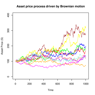
Log-returns are normally distributed in the BSM model; the log-price process follows a standard Brownian motion with drift ([4]). Setting $\mu=0$ eliminates the drift component.
Poisson Process: Let $\lambda>0$ and $\delta_{1}$ be the Dirac measure for $x=1$. Suppose $L_{1}\sim\operatorname{Poisson}(\lambda)$, then the triplet is given by $(0,0,\lambda\delta_{1})$. The density $\eta_{L_{1}}$ is given by,

$$\eta_{L_{1}}(x)=\lambda e^{-\lambda x}.$$ (3.4)

The decomposition is the cumulative sum of jumps up to time $t$, which has a characteristic exponent of the form,

$$\Psi(u)=\lambda(1-e^{iu}).$$ (3.5)

Random variables can be obtained to simulate the path of assets by calling:

#Poisson generator
PPgen=function(lambda){
X=0
Sum=0
flag=0
while (flag==0){
E=-log(runif(1))
Sum=Sum+E
if (Sum < lambda) { X=X+1} else { flag=1}
}
return(X)
}

#Poisson process
PP=function(lambda, N, T){
h=T/N
t=(0:T)/N
X=rep(0, N+1)
I=rep(0,N)
X[1]=0
for(i in 1:N) {
I[i]=PPgen(h*lambda)
X[i+1]=X[i] + I[i]}
return(X)
}

Figure 2: Sample paths of a Poisson process with $\lambda=100$.

Compound Poisson Process: Let $\lambda>0$ be the intensity of a Poisson random variable $N$ and let $\xi_{i}$ be random variables with law $F$ for $i\geq 1$ (independent of N). Suppose $L_{1}$ follows a compound Poisson distribution. Then the triplet is given by $(-\lambda\int_{0<|x|<1}xF(dx),0,\lambda F(dx))$. The density $\eta_{L_{1}}$ is not analytically tractable. The canonical decomposition is given by,

$$L_{t}=\displaystyle\sum_{i=1}^{N_{t}}\xi_{i}$$ (3.6)

which has a characteristic exponent of the form,

$$\Psi(u)=\lambda\int\limits_{\mathbb{R}}(1-e^{iux})F(dx).$$ (3.7)

Random variables can be obtained to simulate the path of assets by calling:

CPP=function(lambda, T, N) {
h=T/N
t=(0:T)/N
X=rep(0, N+1)
F=rep(0, N+1)
I=rep(0,N)
X[1]=0
for(i in 1:N) {
I[i]=PPgen(h*lambda)
if (I[i]==0){F[i]=0} else {F[i]=rnorm(1)}
X[i+1]=X[i] + F[i]}
return(X)
}

Figure 3: Sample paths of a compound Poisson process with $\lambda=100$ and a standard normal jump distribution.

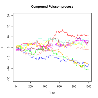
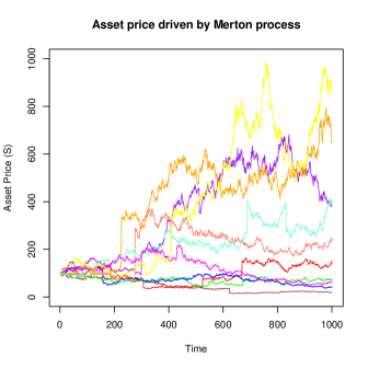
Merton model: Suppose that log-returns $L_{1}$ are determined by the Merton model; the sum of standard Brownian motion (with drift) and a compound Poisson process whose jumps are normally distributed ([22]). Then $\xi_{i}\sim\operatorname{Normal}(\mu_{\xi},\sigma_{\xi})$ for $i\geq 1$ and the triplet is $(\mu,\sigma^{2},\lambda\times\eta_{\xi})$. As expected, the density $\eta_{L_{1}}$ is not analytically tractable. The density $\eta_{\xi}$ is given by,

$$\eta_{\xi}(x)=\frac{1}{\sqrt{2\pi}\sigma_{\xi}}e^{-(x-\mu_{\xi})^{2}/2\sigma_{\xi}^{2}}.$$ (3.8)

The canonical decomposition is given by,

$$L_{t}=\mu t+\sigma W_{t}+\displaystyle\sum_{i=1}^{N_{t}}\xi_{i}$$ (3.9)

which has a characteristic exponent of the form,

$$\Psi(u)=\frac{1}{2}\sigma^{2}u^{2}-iu\mu+\lambda(1-e^{iu\mu_{\xi}-\sigma^{2}_{\xi}u^{2}/2}).$$ (3.10)

which can be obtained via:

Merton_CF=function(u,sigma,a,b,lambda, time){
jump=lambda*time*(-a*u*1i+(exp(u*1i*log(1+a)+0.5*b*b*u*1i*(u*1i-1))-1))
phi=BS_CF(u,sigma,r,time)+exp(jump)
return(phi)
}

Random variables can be obtained to simulate the path of assets by calling:

Merton=function(mu,sigma,lambda,mu_xi,sigma_xi, N, T) {
h=T/N
t=(0:T)/N
X=rep(0, N+1)
F=rep(0, N+1)
I=rep(0,N)
X[1]=0
for(i in 1:N) {
I[i]=PPgen(h*lambda)
if (I[i]==0){F[i]=0} else {F[i]=mu_xi*I[i]+ sqrt(sigma_xi)*sqrt(I[i])*rnorm(1)}
X[i+1]=X[i] + mu*h+sigma*sqrt(h)*rnorm(1)+F[i]}
return(X)
}

Figure 4: Sample paths of an asset driven by a Merton process with $\mu=0.5$, $\sigma=0.75$, and $\lambda=1.5$.

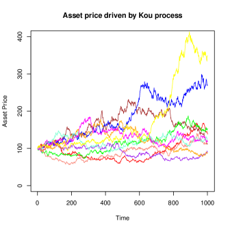
Kou model: Suppose that log-returns $L_{1}$ are determined by the Kou model; the sum of standard Brownian motion (with drift) and a compound Poisson process whose jumps are double-exponentially distributed ([16]). Then $\xi_{i}\sim\operatorname{DExp}(p,\theta_{1},\theta_{2})$ for $i\geq 1$ and the triplet is $(\mu,\sigma^{2},\lambda\times\eta_{\xi})$. Once again, the density $\eta_{L_{1}}$ is not analytically tractable. The density $\eta_{\xi}$ is given by,

$$\eta_{\xi}(x)=p\theta_{1}e^{-\theta_{1}x}\mathds{1}_{\{x<0\}}+(1-p)\theta_{2}e^{\theta_{2}x}\mathds{1}_{\{x>0\}}.$$ (3.11)

The canonical decomposition is given by,

$$L_{t}=\mu t+\sigma W_{t}+\displaystyle\sum_{i=1}^{N_{t}}\xi_{i}$$ (3.12)

which has a characteristic exponent of the form,

$$\Psi(u)=\frac{1}{2}\sigma^{2}u^{2}-iu\mu+\lambda\bigg{(}1+\frac{(1-p)\theta_{2}}{\theta_{2}+iu}-\frac{p\theta_{1}}{\theta_{1}-iu}\bigg{)}.$$ (3.13)

which can be obtained via:

Kou_CF=function(u,sigma, lambda, p, theta_1, theta_2, r, time){
drift=r-0.5*sigma^2 -lambda*(((p*theta_1)/(theta_2+1))+((1-p)*theta_2/(theta_2+1))-1)
phi=exp(1i*u*drift*time-0.5*sigma^2*u*u*time+time*lambda*((p*theta_1)/(theta_1+u*1i)+((1-p)*theta_2)/(theta_2+u*1i)-1))
return(phi)
}

Random variables can be obtained to simulate the path of assets by calling:

Kou=function(mu,sigma,lambda,p,theta_1,theta_2, T, N) {
h=T/N
t=(0:T)/N
X=rep(0, N+1)
F=rep(0, N+1)
I=rep(0,N)
X[1]=0
for(i in 1:N) {
I[i]=PPgen(h*lambda)
if (I[i]==0){F[i]=0}
else {
K=rbinom(1,I[i],p)
R1=rgamma(1,K*theta_1,theta_2)
R2=rgamma(1,(I[i]-K)*theta_1,theta_2)
F[i]=R1-R2}
X[i+1]=X[i] + mu*h+sigma*sqrt(h)*rnorm(1)+F[i]}
return(X)
}

Figure 5: Sample paths of an asset driven by a Kou process with $\mu=0.5$, $\sigma=0.75$, $\lambda=1.5$, $p=0.5$, $\theta_{1}=0.25$, and $\theta_{2}=0.25$.

Jump-diffusion models are generated by processes with a non-zero diffusion component and finite jumps. The above examples are all of this type since $\sigma>0$ and $\nu(dx)<\infty$. If instead $\sigma=0$ and $\nu(dy)=\infty$, we obtain the class of infinite activity pure jump models. The majority of asset pricing models proposed in recent years are of this type.

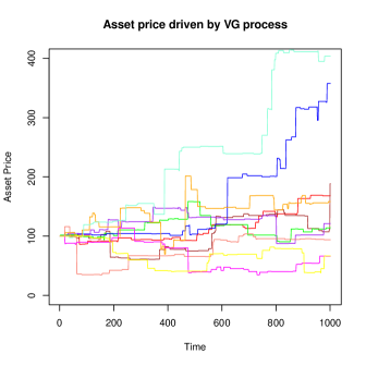
Variance Gamma Process: Suppose that log-returns $L_{1}$ are determined by a variance gamma price process ([18], [21]). The variance gamma process can be obtained by evaluating standard Brownian motion with drift, subordinated by a gamma process in the time variable. Let $\mu,\sigma,v>0$

$$C =\frac{1}{v}>0$$ (3.14)

$$G =\bigg{(}\sqrt{\frac{1}{4}\mu^{2}v^{2}+\frac{1}{2}\sigma^{2}v}-\frac{1}{2}\mu v\bigg{)}^{-1}>0$$ (3.15)

$$M =\bigg{(}\sqrt{\frac{1}{4}\mu^{2}v^{2}+\frac{1}{2}\sigma^{2}v}+\frac{1}{2}\mu v\bigg{)}^{-1}>0.$$ (3.16)

By defining $\gamma=\frac{C}{MG}\big{[}M(e^{-G}-1)-G(e^{-M}-1)\big{]}$ and,

$$\nu^{VG}(dx)=Ce^{G|x|}|x|^{-1}\mathds{1}_{x<0}dx+Ce^{-Mx}x^{-1}\mathds{1}_{x>0}dx$$ (3.17)

the triplet becomes $(\gamma,0,\nu^{VG})$. The density $\eta_{L_{1}}$ is not analytically tractable (page 4, rathgeber, stadler, stockl). The canonical decomposition is given by,

$$L_{t}=t\mathbb{E}[L_{1}]+\int\limits_{0}^{t}\int\limits_{\mathbb{R}}x(\eta^{L}-\nu^{VG})(ds,dx)$$ (3.18)

which has a characteristic exponent of the form,

$$\Psi(u)=\frac{1}{v}\ln\big{[}1-iu\mu v+\frac{1}{2}\sigma^{2}vu^{2}\big{]}.$$ (3.19)

which can be obtained via:

VG_CF=function(u,sigma, theta, nu, r, time){
drift=r+log(1-theta*nu -0.5*sigma*sigma*nu)/nu
phi=exp(1i*drift*time*u) *((1-1i*nu*theta*u+0.5*nu*sigma*sigma*u*u)^(-time/nu))
return(phi)
}

Alternatively, (3.18) can be expressed as the difference between two gamma processes i.e. $L_{t}=G_{t}^{1}-G_{t}^{2}$. The density of a gamma process is given by,

$$\eta_{L_{1}}(x)=\frac{b^{a}}{\Gamma(a)}x^{a-1}e^{-xb}$$ (3.20)

where $a,b,x>0$. By setting $a=C$ and $b=M$ for $G_{t}^{1}$ and $a=C$ and $b=G$ for $G_{t}^{2}$, one can simulate the VG process in this way.

VG=function(sigma, nu, mu, T, N) {
a=1/nu
b=1/nu
h=T/N
t=(0:T)/N
X=rep(0, N+1)
I=rep(0,N)
X[1]=0
for(i in 1:N) {
I[i]=rgamma(1,a*h,b)
X[i+1]=X[i] + mu*I[i]+sigma*sqrt(I[i])*rnorm(1)
}
return(X)
}

Figure 6: Sample paths of an asset driven by a VG process with $\sigma=0.75$, $v=0.5$, and $\mu=0.1$.

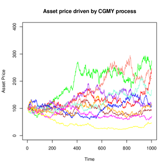
CGMY Process: Suppose that log-returns $L_{1}\sim\operatorname{CGMY}(C,G,M,Y)$ where $C,G,M$ are adopted from (3.14)-(3.16) and $Y<2$ ([6]). This process has infinite activity iff $Y\in[0,2)$. The first moment does not have an explicit form. Let,

$$\nu^{TS}(dx)=\frac{Ce^{-Mx}}{x^{1+Y}}\mathds{1}_{x>0}dx+\frac{Ce^{-G|x|}}{|x|^{1+Y}}\mathds{1}_{x<0}dx$$ (3.21)

then the triplet is given by $(\mathbb{E}[L_{1}],0,\nu^{TS}(dx))$. The density $\eta_{L_{1}}$ is not analytically tractable. The canonical decomposition is given by,

$$L_{t}=t\mathbb{E}[L_{1}]+\int\limits_{0}^{t}\int\limits_{\mathbb{R}}x(\eta^{L}-\nu^{TS})(ds,dx)$$ (3.22)

which has a characteristic exponent of the form,

$$\Psi(u)=C\Gamma(-Y)[G^{Y}+M^{Y}-(M-iu)^{Y}-(G+iu)^{Y}].$$ (3.23)

which can be obtained via:

CGMY_CF=function(u,T,r,C,G,M,Y){
omega=-C*cgamma(-Y)*((M-1)^Y-M^Y+(G+1i*u)^Y-G^Y)
tmp=C*T*cgamma(-Y)*((M-1i*u)^Y-M^Y+(G+1i*u)^Y-G^Y)
phi=exp(1i*u*((r+omega)*T)+tmp)
return(phi)
}

Similar to the VG process, the CGMY process can be simulated using Brownian subordination [19]. Let,

$$A=\frac{G-M}{2}\hskip 14.22636pt{\text{and}}\hskip 14.22636ptB=\frac{G+M}{2}.$$ (3.24)

Then the process defined by $L_{t}=AY_{t}+W(Y_{t})$ is equivalent to (3.22) where $Y_{t}$ is the process with density,

$$\eta_{L_{1}}(x)=\exp\bigg{(}\frac{-(B^{2}-A^{2})y}{2}\bigg{)}\frac{\Gamma(Y)h_{Y}(B\sqrt{y})}{\Gamma(Y/2)2^{Y/2-1}}$$ (3.25)

and for $Y>0$,

$$h_{Y}(z)=\frac{1}{\Gamma(Y)}\int_{0}^{\infty}e^{-y^{2}/2-yz}y^{Y-1}dy.$$ (3.26)

Random variables can be obtained to simulate the path of assets by calling:

CGMY=function(C,G,M,Y, T,N) {
h=T/N
t=(0:T)/N
A=(G-M)/2
B=(G+M)/2
f=function(y){exp(-(B^2-A^2)*y/2)*cgamma(Y)*CGMY_f(y,Y,B)/(cgamma(Y/2)*2^(Y/2-1))}
X=rep(0, N+1)
I=rep(0,N)
probJ=rep(0,N)
J=(0:(N-1))*h + h
for (j in 1:N) {probJ[[j]]<-f(J[[j]])}
randf=sample(J,N,probJ,replace=TRUE)
X[1]=0
for(i in 1:N) {
I[i]=randf[[i]]
X[i+1]=X[i] + A*I[i]+sqrt(I[i])*rnorm(1)
}
return(X)
}

Figure 7: Sample paths of an asset driven by a CGMY process with $C=5$, $G=25$, $M=25$, and $Y=1$.

Generalized Hyperbolic Process: Suppose that log-returns $L_{1}\sim\operatorname{GH}(\alpha,\beta,\delta,\mu,\lambda)$ ([9], [26], [2]). The parameter $\alpha>0$ determines the shape, $0\leq|\beta|<\alpha$ determines the skewness, $\mu\in\mathbb{R}$ gives the location, $\delta>0$ is the scaling parameter, and $\lambda\in\mathbb{R}$ determines the heaviness of the tails. The first moment is given by,

$$\mathbb{E}[L_{1}] =\mu+\frac{\beta\delta^{2}K_{\lambda+1}(\zeta)}{\zeta K_{\lambda}(\zeta)}$$ (3.27)

where $\zeta=\delta\sqrt{\alpha^{2}-\beta^{2}}$. By defining

$$\nu^{GH}(dx) =\frac{e^{\beta x}}{|x|}\Bigg{(}\int\limits_{0}^{\infty}\frac{e^{-\sqrt{2y+\alpha^{2}}|x|}}{\pi^{2}y(J_{|\lambda|}^{2}(\delta\sqrt{2y})+Y_{|\lambda|}^{2}(\delta\sqrt{2y})}dy+\lambda e^{-\alpha|x|}\mathds{1}_{\{\lambda\geq 0\}}\Bigg{)}$$ (3.28)

the triplet is given by $(\mathbb{E}[L_{1}],0,\nu^{GH}(dx))$. The density $\eta_{L_{1}}$ is known:

$$\eta_{L_{1}}(x)=c(\alpha,\beta,\delta,\lambda)[\delta^{2}+(x-\mu)^{2}]^{(\lambda-\frac{1}{2})/2}K_{\lambda-\frac{1}{2}}(\alpha\sqrt{\delta^{2}+(x-\mu)^{2}})e^{\beta(x-\mu)}$$ (3.29)

where

$$c(\alpha,\beta,\delta,\lambda)=\frac{(\alpha^{2}-\beta^{2})^{\frac{\lambda}{2}}}{\sqrt{2\pi}\alpha^{\lambda-\frac{1}{2}}K_{\lambda}(\delta\sqrt{\alpha^{2}-\beta^{2}})}.$$ (3.30)

The canonical decomposition is given by,

$$L_{t}=t\mathbb{E}[L_{1}]+\int\limits_{0}^{t}\int\limits_{\mathbb{R}}x(\eta^{L}-\nu^{GH})(ds,dx)$$ (3.31)

which has a characteristic exponent of the form,

$$\Psi(u)=-\ln\bigg{[}\bigg{(}\frac{\alpha^{2}-\beta^{2}}{\alpha^{2}-(\beta+iu)^{2}}\bigg{)}^{\frac{\lambda}{2}}\frac{K_{\lambda}(\delta\sqrt{\alpha^{2}-(\beta+iu)^{2}})}{K_{\lambda}(\delta\sqrt{\alpha^{2}-\beta^{2}})}\bigg{]}-iu\mu.$$ (3.32)

which can be obtained via:

GH_CF=function(u,T,r,alpha, beta, delta, nu){
arg1=alpha*alpha-beta*beta
arg2=arg1-2*1i*u*beta+u*u
argm=arg1-2*beta-1
omega= - log((arg1/argm)^(0.5*nu)*BesselK(delta*sqrt(argm),nu)/BesselK(delta*sqrt(arg1), nu))
tmp=(arg1/arg2)^(0.5*nu)*BesselK(delta*sqrt(arg2), nu)/BesselK(delta*sqrt(arg1), nu)
phi=exp(1i*u*((r+omega)*T)+log(tmp)*T)
return(phi)
}

A natural way to simulate the GH process is to directly compute,

$$L_{t}=\mu+\beta Y_{t}+W(Y_{t}).$$ (3.33)

where $Y_{t}$ is a random variable from a generalized inverse Gaussian (GIG) distribution. The density of the GIG distribution is given by,

$$\eta_{L_{1}}(x)=\frac{(a/b)^{p/2}}{2K_{p}(\sqrt{ab})}x^{p-1}e^{-(ax+b/x)/2}$$ (3.34)

where $a,b,x>0$, $p\in\mathbb{R}$, and $K_{p}$ is a modified Bessel function of the second kind. By setting $a=\alpha^{2}-\beta^{2}$, $b=\delta^{2}$, and $p=\lambda$ we obtain the density of $Y$. Random variables can be obtained to simulate the path of assets by calling:

GH=function(alpha,beta,delta,lambda,mu, T, N){
h=T/N
t=(0:T)/N
I=rep(0, N)
X=rep(0, N+1)
for (i in 1:N) {
I[i] = rgig(1, lambda,  h*sqrt(alpha*alpha-beta*beta),delta)
X[i+1]=X[i]+mu/N+beta*I[i]+ sqrt(I[i])*rnorm(1)
}
return(X)
}

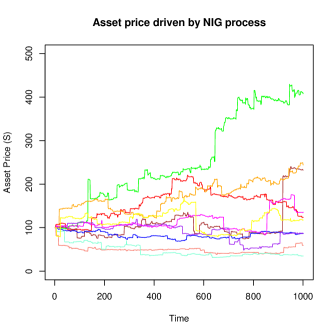
Normal Inverse Gaussian Process: By setting $\lambda=-\frac{1}{2}$ for the GH process, we obtain the NIG ([3]). The Lévy triplet is inherited from before as $(\mathbb{E}[L_{1}],0,\nu^{NIG}(dx))$ where the first moment is given by,

$$\mathbb{E}[L_{1}]=\mu+\frac{\beta\delta}{\sqrt{\alpha^{2}-\beta^{2}}}$$ (3.35)

and the measure is defined as,

$$\nu^{NIG}(dx)=e^{\beta x}\frac{\delta\alpha}{\pi|x|}K_{1}(\alpha|x|)dx.$$ (3.36)

Furthermore, the canonical decomposition is given similarly by,

$$L_{t}=t\mathbb{E}[L_{1}]+\int\limits_{0}^{t}\int\limits_{\mathbb{R}}x(\eta^{L}-\nu^{NIG})(ds,dx)$$ (3.37)

which has a characteristic exponent of the form,

$$\Psi(u)=\delta\big{[}\sqrt{\alpha^{2}-(\beta^{2}+iu)^{2}}-\sqrt{\alpha^{2}-\beta^{2}}\big{]}-iu\mu.$$ (3.38)

NIG_CF=function(u,time, r,alpha,beta,delta,mu){
omega=delta*(sqrt(alpha*alpha-(beta+1)^2)-sqrt(alpha*alpha-beta*beta))
tmp=1i*u*mu*time-delta*time*(sqrt(alpha*alpha-(beta+1i*u)^2)-sqrt(alpha*alpha-beta*beta))
phi=exp(1i*u*((r+omega)*T)+tmp)
return(phi)
}

Random variables can be obtained to simulate the path of assets by calling:

#NIG process
NIG=function(alpha,beta,delta,mu, T, N){
a=1
b=delta*sqrt(alpha*alpha-beta*beta)
h=T/N
t=(0:T)/N
I=rep(0, N)
X=rep(0, N+1)
X[1]=0
for (i in 1:N) {
I[i] = IG2(a*h, b)
X[i+1]=X[i]+mu/N+beta*delta*delta*I[i]+ delta*sqrt(I[i])*rnorm(1)
}
return(X)
}

Figure 8: Sample paths of an asset driven by a NIG process with $\alpha=2$, $\beta=1$, $\delta=1.5$, and $\mu=0$.

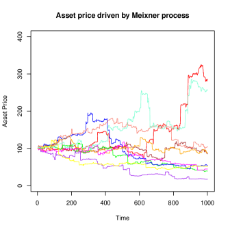
Meixner Process: Let $\alpha,\delta>0$ and $-\pi<\beta<\pi$ so that $L_{1}\sim\operatorname{MX}(\alpha,\beta,\delta)$ ([30], [29]). Define,

$$\nu^{MX}(dx)=\frac{\delta e^{\frac{\beta x}{\alpha}}}{x\sinh(\frac{\pi x}{\alpha})}$$ (3.39)

then similar to the other pure jumps models, the triplet is given by $(\mathbb{E}[L_{1}],0,\nu^{MX})$. The density $\eta_{L_{1}}$ is,

$$\eta_{L_{1}}(x)=\frac{\big{(}2\cos\big{(}\frac{\beta}{2}\big{)}\big{)}^{2\delta}}{2\alpha\pi\Gamma(2\delta)}\big{|}\Gamma\big{(}\delta+\frac{ix}{\alpha}\big{)}\big{|}e^{\frac{\beta x}{\alpha}}.$$ (3.40)

The canonical decomposition is given by,

$$L_{t}=t\mathbb{E}[L_{1}]+\int\limits_{0}^{t}\int\limits_{\mathbb{R}}x(\eta^{L}-\nu^{MX})(ds,dx)$$ (3.41)

which has a characteristic exponent of the form,

$$\Psi(u)=\bigg{(}\frac{\cos(\frac{\beta}{2})}{\cosh(\frac{\pi x}{\alpha})}\bigg{)}^{2\delta}.$$ (3.42)

MX_CF=function(u,T,r,alpha, beta, delta){
omega=-2*delta*(log(cos(0.5*beta))-log(cos((alpha+beta)/2)))
tmp=(cos(0.5*beta)/cosh(0.5*(alpha*u-1i*beta)))^(2*T*delta)
phi=exp(1i*u*((r+omega)*T)+log(tmp))
return(phi)
}

For simulation of the process via Brownian subordination, see [19]. Alternatively, for a simulation method based on acceptance-rejection sampling, see [14]. Random variables can be obtained to simulate the path of assets by calling:

MX=function(alpha, delta, T, N) {
h=T/N
X=rep(0,N+1)
for (i in 1:N){X[[i+1]]=X[[i]]+rmeixner(h,alpha,0,delta)}
return(X)
}

#Meixner Increment Generator
rmeixner = function(t,a,m,r) {
b=0
  r=t*r
  m=t*m
  repeat {
    Q = runif(1,min=-1,max=1)/runif(1,min=-1,max=1)
    V = a/2*max(sqrt(2*r),2*r)*Q
    U = runif(1)
    if (abs(Q) < 1) {
      if (gamma(r)^2*U < abs(cgamma(r+1i*V/a))^2) {
        break
      }
    }
    else {
      if (!is.na(cgamma(r+1i*V/a)))
        if (max(1,2*r)*a^2*gamma(r+1)^2*U/(2*r) < abs(cgamma(r+1i*V/a))^2 *V^2){
             break
           }
    }
  }
  return(V+m)
}

Figure 9: Sample paths of an asset driven by a MX process with $\alpha=0.5$, $\beta=0$, and $\delta=4$.

For a more detailed discussion on Lévy processes, including their applications in finance, see [17], [27], [24], [28], [23], [1].

Should there be errors in this draft, please check with published references for the correct formulations.

References

- [1] D. Applebaum. Lévy Processes and Stochastic Calculus. Cambridge Studies in Advanced Mathematics. Cambridge University Press, 2004.
- [2] O. Barndorff-Nielsen. Exponentially decreasing distributions for the logarithm of particle size. Proceedings of the Royal Society of London. A. Mathematical and Physical Sciences, 353(1674):401–419, 1977.
- [3] O.E. Barndorff-Nielsen. Normal/inverse Gaussian Processes and the Modelling of Stock Returns. Research Reports - Department of Theoretical Statistics, Institute of Mathematics. University of Aarhus. Department, Inst., Univ., 1995.
- [4] Fischer Black and Myron Scholes. The pricing of options and corporate liabilities. Journal of Political Economy, 81(3):637, 1973.
- [5] Peter Carr, Hélyette Geman, Dilip B. Madan, and Marc Yor. The fine structure of asset returns: An empirical investigation, 2000.
- [6] Peter Carr, Hélyette Geman, Dilip B. Madan, and Marc Yor. Stochastic volatility for lévy processes, 2001.
- [7] John C. Cox and Stephen A. Ross. The valuation of options for alternative stochastic processes. Journal of Financial Economics, 3(1-2):145–166, 1976.
- [8] Ernst Eberlein and Ulrich Keller. Hyperbolic distributions in finance. Bernoulli, 1:281–299, 1995.
- [9] Ernst Eberlein and Karsten Prause. The generalized hyperbolic model: Financial derivatives and risk measures. In Mathematical Finance – Bachelier Congress 2000, Geman, pages 245–267. Springer, 1998.
- [10] A. Einstein. Über die von der molekularkinetischen theorie der wärme geforderte bewegung von in ruhenden flüssigkeiten suspendierten teilchen. Annalen der Physik, 322(8):549–560, 1905.
- [11] J.I. Gichman, A.V. Skorochod, and K. Wickwire. Stochastic Differential Equations. 1972.
- [12] I.I Gihman and A.V. Skorokhod. Controlled Stochastic Processes. Springer-Verlag, New York, 1979.
- [13] Ioannis Karatzas and Steven E. Shreve. Brownian Motion and Stochastic Calculus (Graduate Texts in Mathematics). Springer, 2nd edition, August 1991.
- [14] Reiichiro Kawai. Likelihood ratio gradient estimation for Meixner distribution and Lévy processes. Computational Statistics, 27(4):739–755, 2012.
- [15] U. Keller. Realistic Modelling of Financial Derivatives. University of Freiburg/Breisgau, 1997.
- [16] S. G. Kou. A jump-diffusion model for option pricing. Manage. Sci., 48(8):1086–1101, August 2002.
- [17] A.E. Kyprianou. Introductory Lectures on Fluctuations of Lévy Processes with Applications. Universitext (En ligne). Springer-Verlag Berlin Heidelberg, 2006.
- [18] D. Madan, E. Seneta, and University of Sydney. Dept. of Econometrics. Chebyshev Polynomial Approximations and Characteristic Function Estimation. Econometrics discussion papers. Department of Econometrics, University of Sydney, 1986.
- [19] Dilip Madan and Marc Yor. Representing the CGMY and Meixner Lévy processes as time changed Brownian motions. Journal of Computational Finance, 12:1.
- [20] Dilip B. Madan, Peter Carr, and Eric C. Chang. The variance gamma process and option pricing. European Finance Review, 2:79–105, 1998.
- [21] Dilip B. Madan and Eugene Seneta. The variance gamma model for share market returns. The Journal of Business, 63(4):pp. 511–524, 1990.
- [22] Robert C. Merton. Option pricing when underlying stock returns are discontinuous. Journal of Financial Economics, 3:125–144, 1976.
- [23] Antonis Papapantoleaon. An introduction to Lévy processes with applications in finance. Probability Surveys, pages 1–55, 2008.
- [24] A. Papapantoleon. Applications of Semimartingales and Lévy Processes in Finance: Duality and Valuation. 2006.
- [25] A. Papapantoleon. An introduction to Lévy processes with applications in finance. ArXiv e-prints, April 2008.
- [26] K. Prause. The Generalized Hyperbolic Model: Estimation, Financial Derivatives and Risk Measures. 1999.
- [27] P. Protter. Stochastic Integration and Differential Equations: Version 2.1. Applications of Mathematics. Springer, 2004.
- [28] S. Raible. Lévy Processes in Finance: Theory, Numerics, and Empirical Facts. 2000.
- [29] W. Schoutens. The Meixner process: Theory and applications in finance. EURANDOM Report 2002-2004, 2002.
- [30] Wim Schoutens and Jozef L. Teugels. Lévy processes, polynomials and martingales. Communications in Statistics. Stochastic Models, 14(1-2):335–349, 1998.
- [31] P. Tankov. Financial Modelling with Jump Processes, Second Edition. Chapman & Hall/CRC Financial Mathematics Series. Taylor & Francis, 2003.