Heat Conductivity of the Heisenberg Spin-$1/2$ Ladder:
From Weak to Strong Breaking of Integrability

Abstract

We investigate the heat conductivity $\kappa$ of the Heisenberg spin-$1/2$ ladder at finite temperature covering the entire range of inter-chain coupling $J_{\perp}$, by using several numerical methods and perturbation theory within the framework of linear response. We unveil that a perturbative prediction $\kappa\propto J_{\perp}^{-2}$, based on simple golden-rule arguments and valid in the strict limit $J_{\perp}\to 0$, applies to a remarkably wide range of $J_{\perp}$, qualitatively and quantitatively. In the large $J_{\perp}$-limit, we show power-law scaling of opposite nature, namely, $\kappa\propto J_{\perp}^{2}$. Moreover, we demonstrate the weak and strong coupling regimes to be connected by a broad minimum, slightly below the isotropic point at $J_{\perp}=J_{\parallel}$. Reducing temperature $T$, starting from $T=\infty$, this minimum scales as $\kappa\propto T^{-2}$ down to $T$ on the order of the exchange coupling constant. These results provide for a comprehensive picture of $\kappa(J_{\perp},T)$ of spin ladders.

Introduction. Thermodynamic properties of quantum many-body systems are well understood, particularly in the vicinity of integrable points johnston2000 . In contrast, the vast majority of dynamical questions in these systems remain a challenge to theoretical and experimental physics as well, in the entire range from weak to strong breaking of integrability. These questions consist of several timely and important issues such as eigenstate thermalization deutsch1991 ; srednicki1994 ; rigol2008 in cold atomic gases and, as studied in this Letter, quantum transport and relaxation in condensed-matter materials. In this context, a fundamental system is the one-dimensional (1D) spin-$1/2$ Heisenberg model. It is relevant to the physics of quasi-1D quantum magnets johnston2000 , cold atoms in optical lattices trotzky2008 , nanostructures gambardella2006 , and to physical situations in a much broader context kruczenski2004 ; kim1996 .

As typical for integrable systems, the energy current in the spin-$1/2$ Heisenberg chain is a strictly conserved quantity zotos1997 ; kluemper2002 . This implies purely ballistic flow of heat at any temperature and provides the theoretical basis for explaining the colossal magnetic heat conduction observed experimentally in quasi-1D cuprates sologubenko2000 ; hess2001 ; hess2007 ; hlubek2010 . In contrast to heat flow, spin dynamics, including the existence of ballistic shastry1990 ; narozhny1998 ; zotos1999 ; benz2005 ; fujimoto2003 ; prosen2011 ; prosen2013 ; herbrych2011 ; karrasch2012 ; karrasch2013-1 ; steinigeweg2014-1 ; steinigeweg2014-2 ; carmelo2014 and diffusive transport channels sirker2009 ; sirker2011 ; grossjohann2010 ; znidaric2011 ; steinigeweg2011 ; karrasch2014 , is theoretically resolved only partially, and also under ongoing experimental scrutiny thurber2001 ; maeter2012 ; ronzheimer2013 ; hild2014 ; xiao2014 .

Figure 1: (Color online) Thermal conductivity $\kappa$ (per chain) versus $J_{\perp}/J_{\parallel}$ and $\beta$. PT: known perturbative regime. Issues clarified in this Letter: extent of power-law scaling (dashed line) close to PT and sum-rule (SR) regimes, nonperturbative numerical treatment for entire $J_{\perp}$-range, location of minimal conductivity, and temperature variation.

Because of strict energy-current conservation in this model, the heat conductivity $\kappa$ is highly susceptible to breaking of integrability by, e.g., spin-phonon coupling shimshoni2003 ; rozhkov2005 ; hlubek2012 , dimerization or disorder huang2013 ; karrasch2013-2 ; karahalios2009 , and interactions between further neighbors heidrichmeisner2003 ; steinigeweg2013 . One of the most important perturbations is inter-chain coupling, i.e. $J_{\perp}$, which is the key ingredient to spin-ladder compounds sologubenko2000 ; hess2001 . Since the discovery of the discontinuous transition from one to two dimensions in quantum magnets Elbio1996 , spin ladders are a cornerstone of correlated electron systems. They display quantum confinement Bella2010a , transforming gapless spinons of simple spin chains into new massive triplons Notbohm2007 ; Schmidiger2013 . They provide insights into fractionalization, quantum phase transitions Thielemann2009a , Bose-Einstein condensation Thielemann2009b , and disorder-induced magnetism George1997a . They are paradigmatic to high-T_C superconductors, undoped Tranquada2004 and doped Elbio1992 . They serve as models in other fields, e.g., cold atomic gases Garcia2004 , quantum information theory Ying2005 , and carbon nanotubes Deshpande2009 .

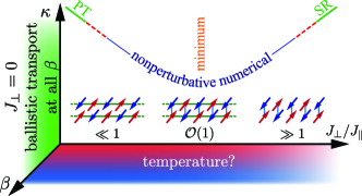
Early on, perturbation theory (PT) to lowest order, i.e., a simple golden-rule argument jung2006 ; jung2007 , has suggested dissipative heat flow with a scaling $\kappa\propto J_{\perp}^{-2}$, as illustrated on the l.h.s. of Fig. 1. However, the relevance of such scaling is unclear off the strict limit $J_{\perp}\to 0$, as is the radius of convergence of the PT. Understanding $\kappa$ over a wider $J_{\perp}$ range has been hampered by the lack of sufficiently accurate nonperturbative methods. In particular, state-of-the-art numerical methods have been restricted to the regime $J_{\perp}={\cal O}(1)$, where finite-size effects are moderate and spectral structures are broad, i.e., time scales are short zotos2004 ; note . Thus, heat transport in the transition from weakly coupled chains to strongly coupled ladders is understood only in few and narrow regions.

In this Letter, we lift these restrictions and study the heat conductivity $\kappa$ over the entire range of the inter-chain coupling $J_{\perp}$. Using several methods within linear response, we (a) quantitatively connect to PT in the small-$J_{\perp}$ limit and (b) unveil its validity for a remarkably wide range of $J_{\perp}$. In addition to the PT, scaling as $\kappa\propto J_{\perp}^{-2}$, we (c) demonstrate a qualitatively different power-law scaling $\kappa\propto J_{\perp}^{2}$ in the large $J_{\perp}$-limit. Consequently, we (d) find a broad minimum of $\kappa$ in the region $J_{\perp}\lesssim 1$. Reducing temperature $T$, starting from $T=\infty$, this minimum (e) scales as $\kappa\propto T^{-2}$ down to $T$ on the order of the exchange coupling. Thus, we provide a comprehensive picture of $\kappa(J_{\perp},T)$, beyond the known results sketched as part of Fig. 1.

Model. We study a Heisenberg spin-$1/2$ ladder of length $N/2$ with periodic boundary conditions. The Hamiltonian $H=H_{\parallel}+H_{\perp}$ consists of a leg part $H_{\parallel}$ and a rung part $H_{\perp}$,

$$H_{\parallel}=J_{\parallel}\!\sum_{k=1}^{z}\sum_{i=1}^{N/2}\mathbf{S}_{i,k}\cdot\mathbf{S}_{i+1,k}\,,\,\,H_{\perp}=J_{\perp}\!\sum_{i=1}^{N/2}\mathbf{S}_{i,1}\cdot\mathbf{S}_{i,2}\,,$$ (1)

where $\mathbf{S}_{i,k}$ are spin-1/2 operators at site $(i,k)$, $J_{\parallel}>0$ is the antiferromagnetic leg coupling, and $J_{\perp}>0$ is the rung interaction. $z=2$ is the number of legs. For $J_{\perp}=0$, the ladder splits into integrable chains, with a gapless ground state and spinon excitations. For $J_{\parallel}=0$, it simplifies to uncoupled dimers, with a gapped ground state and triplon excitations. For $J_{\perp},J_{\parallel}\neq 0$, the ladder is nonintegrable. Generally, the model in Eq. (1) preserves the total magnetization $S^{z}$ and is translationally invariant. We focus on the representative sector $S^{z}=0$ SM .

The energy current has the well-known form $j=j_{\parallel}+j_{\perp}$ zotos2004 ,

$$j_{\parallel}=J_{\parallel}^{2}\sum_{k=1}^{z}\sum_{i=1}^{N/2}\mathbf{S}_{i-1,k}\cdot(\mathbf{S}_{i,k}\times\mathbf{S}_{i+1,k})\,,$$ (2)

$$j_{\perp}=\frac{J_{\parallel}J_{\perp}}{2}\sum_{k=1}^{z}\sum_{i=1}^{N/2}(\mathbf{S}_{i-1,k}-\mathbf{S}_{i+1,k})\cdot(\mathbf{S}_{i,k}\times\mathbf{S}_{i,3-k})\,.$$

$j$ and $H$ commute only at the integrable point $J_{\perp}=0$. We investigate the autocorrelation function at inverse temperatures $\beta=1/T$,

$$C(t)=\text{Re}\frac{\langle j(t)\,j\rangle}{N}=\text{Re}\frac{\text{Tr}\{e^{-\beta H}j(t)\,j\}}{N\,\text{Tr}\{e^{-\beta H}\}}\,,$$ (3)

where the time argument of $j(t)$ refers to the Heisenberg picture, $j=j(0)$, and $C(0)=3(J_{\parallel}^{4}+J_{\parallel}^{2}J_{\perp}^{2}/2)/32$ for $\beta J_{\parallel}\to 0$.

From $C(t)$, we first determine the Fourier transform $C(\omega)$ and then the conductivity via the low-frequency limit $\kappa/z=\beta^{2}C(\omega\to 0)$. Additionally, we can extract the conductivity directly by $\kappa/z=\beta^{2}\int_{0}^{t_{1}}\text{d}t\,C(t)$. Here, the cut-off time $t_{1}$ has to be chosen much larger than the relaxation time $\tau$, where $C(\tau)/C(0)=1/e$ steinigeweg2014-3 .

Methods. We calculate $C$ by complementary numerical methods, with a particular focus on dynamical quantum typicality (DQT) elsayed2013 ; steinigeweg2014-1 ; steinigeweg2014-2 (see also Refs. gemmer2003, ; goldstein2006, ; popescu2006, ; reimann2007, ; white2009, ; bartsch2009, ; bartsch2011, ; sugiura2012, ; hams2000, ). DQT relies on the time-domain relation

$$C(t)=\text{Re}\frac{\langle\Phi_{\beta}(t)|j|\varphi_{\beta}(t)\rangle}{N\,\langle\Phi_{\beta}(0)|\Phi_{\beta}(0)\rangle}+\epsilon\,,$$ (4)

$|\Phi_{\beta}(t)\rangle=e^{-\imath Ht-\beta H/2}\,|\psi\rangle$, $|\varphi_{\beta}(t)\rangle=e^{-\imath Ht}\,j\,e^{-\beta H/2}\,|\psi\rangle$, where $|\psi\rangle$ is a single pure state drawn at random and $\epsilon$ scales inversely with the partition function, i.e., $\epsilon$ is exponentially small in the number of thermally occupied eigenstates elsayed2013 ; steinigeweg2014-1 ; steinigeweg2014-2 . The great advantage of Eq. (4) is that it can be calculated without any diagonalization by the use of forward-iterator algorithms. We use a fourth-order Runge-Kutta iterator with a discrete time step $\delta tJ_{\parallel}=0.01\ll 1$. Together with sparse-matrix representations of operators, we can reach systems sizes as large as $N=32$. For more details on the method and its accuracy, see Refs. steinigeweg2014-2, ; SM, .

Additionally, we confirm our DQT results with numerical methods based on Lanczos diagonalization in the frequency domain prelovsek2013 , with the frequency resolution $\delta\omega$ crucially depending on the number of Lanczos steps $M$, $\delta\omega\propto 1/M$. At low $T$, we choose the finite-$T$ Lanczos method (FTLM) with $M\sim 200$ SM . At high $T$, we also use the microcanonical Lanczos method (MCLM) with $M\sim 2000$, significantly improving $\delta\omega$.

Figure 2: (Color online) The (a) $t$ and (b) $\omega$ dependence of the autocorrelation $C$ for strong $J_{\perp}/J_{\parallel}\geq 1$, $\beta J_{\parallel}\to 0$, and $N\leq 32$, as obtained from DQT. Spectra in (b) are obtained by Fourier transforming finite-$t$ data $t\leq 10\tau\sim 20/J_{\parallel}$ (symbols); Inset: Low-$\omega$ limit for $J_{\perp}/J_{\parallel}=1$, the largest $N=32$, and $t\leq 5\tau$ (crosses), $10\tau$ (other symbols), $50\tau$ (curves); Main panel: Spectra from Lanczos methods ($N=28$ MCLM of Ref. zotos2004, , $N=22$ FTLM) are shown (curves). Note that method-related errors are negligibly small SM .

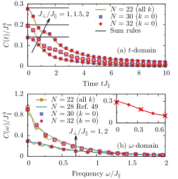
Results. We begin with $J_{\perp}/J_{\parallel}\geq 1$ and $\beta J_{\parallel}\to 0$. In Fig. 2 (a) we summarize our DQT results on $C(t)$ for different $J_{\perp}/J_{\parallel}=1$, $1.5$, $2$. Several comments are in order. First, the initial value $C(0)$ agrees with the high-$T$ sum rule and therefore increases with $J_{\perp}$. Second, all $C(t)$ depicted decay to zero on a time scale $5\tau\sim 10/J_{\parallel}$. Third, the $C(t)$ curves do not change when the number of sites is increased from $N=22$ to $32$. Thus, we observe very little finite-size effects, i.e., we can safely consider our results as results on $C(t)$ for $N\to\infty$. Note that for $N\geq 30$ we consider a single translation subspace $k$ since, for these $N$, $C(t)$ is $k$ independent at $\beta\to 0$ steinigeweg2014-1 ; steinigeweg2014-2 .

Next, we discuss the spectrum $C(\omega)$. To this end, we show in Fig. 2 (b) for $J_{\perp}/J_{\parallel}=1$, $2$ the Fourier transform of our DQT data for times $t\leq 10\tau\sim 20/J_{\parallel}$. These times correspond to a frequency resolution $\delta\omega\sim 0.15J_{\parallel}$. For this resolution, the Fourier transform is a smooth function of $\omega$ and displays a well-behaved limit for $\omega\to 0$, i.e., $C(\omega\to 0)=C(\omega=0)$. Moreover, this limit and $C(\omega)$ in general do not depend on system size for $N\geq 22$. The inset of Fig. 2 (b) clarifies the impact of the $\omega$ resolution by displaying additional Fourier transforms of DQT data, evaluated for shorter ($t\leq 5\tau$) and longer ($t\leq 50\tau$) times at $J_{\perp}/J_{\parallel}=1$ and for the largest $N=32$. Clearly, the low-$\omega$ limit is independent of the $\omega$ resolution resulting from the specific choice of $t$. This robustness, together with the $N$ independence, allows us to reliably extract a quantitative value for the dc conductivity at $J_{\perp}/J_{\parallel}=1$, $\kappa/z\beta^{2}J_{\parallel}^{3}=0.29$.

To additionally demonstrate the validity of our DQT approach, we compare to our FTLM results and to existing MCLM spectra from the literature zotos2004 in Fig. 2 (b). Obviously, the agreement is very good.

Figure 3: (Color online) (a) The $t$ dependence of $C$ for various small $J_{\perp}/J_{\parallel}=0.15$, …, $0.75$, obtained from DQT for $\beta J_{\parallel}\to 0$ and $N\leq 30$. (b) Spectrum for $J_{\perp}/J_{\parallel}=0.25$, obtained by Fourier transforming finite-$t$ data $t\leq 5\tau\sim 80/J_{\parallel}$ (symbols); Inset: Low-$\omega$ limit for the largest $N=32$ and $t\leq 5\tau$ (diamonds), $10\tau$ (crosses); Main panel: Spectrum from $N=22$ and $28$ MCLM and a Lorentzian fit are shown (curves).

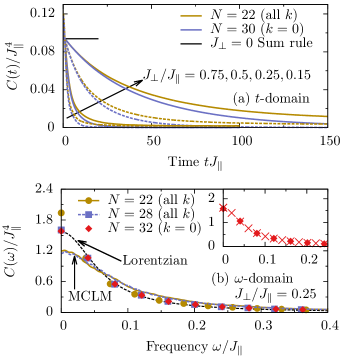
Now, we turn to small $J_{\perp}/J_{\parallel}<1$. In Fig. 3 (a) we depict our DQT results on $C(t)$ for various $J_{\perp}/J_{\parallel}=0.15,\ldots,0.75$. The initial value $C(0)$ approaches the $J_{\perp}=0$ sum rule when $J_{\perp}$ is reduced. Furthermore, the decay is slower for smaller $J_{\perp}$ and finite-size effects are naturally stronger in the vicinity of the integrable point $J_{\perp}=0$. For the smallest $J_{\perp}/J_{\parallel}=0.15$ depicted, these finite-size effects are still moderate when comparing $C(t)$ for $N=22,30$. In Fig. 3 (b) we show the Fourier transform of $C(t\leq 5\tau\sim 80J_{\parallel})$ for $J_{\perp}/J_{\parallel}=0.25$. For the largest $N=32$, this Fourier transform is well described by a Lorentzian line shape and, again, the low-$\omega$ limit does not depend on $t$. Since $C(\omega)$ has a narrow spectrum, MCLM with a high $\omega$ resolution ($M=2000$) is a better choice for comparison than FTLM ($M=200$) SM , and agrees well with DQT. Note that resolving narrow spectral features by DQT is a new concept of our Letter, which can be applied in a much broader context.

Figure 4: (Color online) (a) Scaling of the conductivity $\kappa$ with $J_{\perp}$, obtained from DQT and finite-$t$ data $t\leq 5\tau$ for $\beta J_{\parallel}\to 0$ and $N\leq 32$ (closed symbols). Results for the simplified operator $j^{\prime}=j_{\parallel}$ are also depicted at $J_{\perp}/J_{\parallel}\sim 1$ (open symbols). Additionally, power laws $0.097(J_{\perp}/J_{\parallel})^{-2}$ and $0.21(J_{\perp}/J_{\parallel})^{2}$ are shown (lines). (b) PT for the scattering rate $\gamma$, carried out using DQT. The PT of Ref. jung2006, is also depicted (bullet).

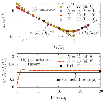
Next, we discuss the scaling of the conductivity $\kappa$ over the entire range of $J_{\perp}$. In Fig. 4 (a) we summarize $\kappa(J_{\perp})$ as inferred from DQT data for $C(t\leq 5\tau)$. Here, we observe a broad minimum of $\kappa(J_{\perp})$, centered between two regimes with power-law scaling at large and small $J_{\perp}$. The scaling $\propto J_{\perp}^{2}$ in the large $J_{\perp}$ limit is a direct consequence of the static sum rule $C(0)\propto J_{\perp}^{2}$, noted following Eq. (3). The scaling $\propto J_{\perp}^{-2}$ for small $J_{\perp}$, however, is not simply related to $C(0)$ since $C(0)\approx\text{const.}$ for such $J_{\perp}$. Particularly, we find this scaling to hold over a remarkably wide range of $0.07\leq J_{\perp}/J_{\parallel}\lesssim 0.35$. This finding is a central result of this Letter. Below $J_{\perp}/J_{\parallel}<0.07$, computational efforts for $5\tau$ data are very high and finite-size effects are too large, even for N accessible to DQT.

To gain further insight into the scaling at small $J_{\perp}$, we calculate the scattering rate $\gamma=1/\tau$ to lowest order in $J_{\perp}$, i.e., $J_{\perp}^{2}$, following the PTs in Refs. jung2006, ; jung2007, ; steinigeweg2010, ; steinigeweg2011-1, . This rate reads ($\beta J_{\parallel}\to 0$)

$$\gamma=\lim_{t_{1}\to\infty}\int_{0}^{t_{1}}\!\text{d}t_{\parallel}\frac{\text{Tr}\{\imath[j_{\parallel},H_{\perp}](t_{\parallel})\,\imath[j_{\parallel},H_{\perp}]\}}{\text{Tr}\{j_{\parallel}^{2}\}}\propto J_{\perp}^{2}\,,$$ (5)

where $t_{\parallel}$ refers to the Heisenberg picture of $H_{\parallel}$. Figure 4 (b) shows $\gamma$ evaluated by DQT applied to Eq. (5) for large $N\leq 30$. Note that this application of DQT is a new concept of our Letter SM . As shown in Fig. 4, we find good agreement with previous evaluation of $\gamma$ in Ref. jung2006, based on smaller systems. Most notably, however, $\gamma$ well agrees with the scattering rate $\gamma^{\prime}$ as extracted directly from $\kappa$ in Fig. 4 (a) via the relation $\gamma^{\prime}=z\beta^{2}C(0)/\kappa$. This agreement is another main result of our Letter. Note that PT holds up to $J_{\perp}/J_{\parallel}\sim 1$ for the simplified current $j=j_{\parallel}$, see Fig. 4 (a), which is the regime where the system behaves Markovian, i.e., has no memory. For the explicit calculation of the memory kernel, see Ref. SM, .

Figure 5: (Color online) (a) The $t$ dependence of $C$ for $\beta J_{\parallel}=0.5,\ldots,1.5$, obtained from DQT for $J_{\perp}/J_{\parallel}=1$ and $N=28$. (b) Spectrum for $\beta J_{\parallel}=1$, obtained by Fourier transforming finite-$t$ data $t\leq 5\tau\sim 12/J_{\parallel}$ for $N\leq 32$. Additionally, a spectrum from $N=22$ FTLM is depicted (curve). Inset: $T$ dependence of the conductivity $\kappa$, calculated by $N=32$ DQT (closed symbols, curve) and $N=22$ FTLM (open symbols).

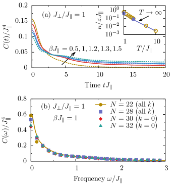
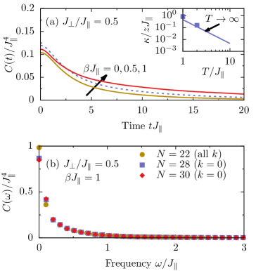
Now we turn to $\beta J_{\parallel}\neq 0$, focusing on $J_{\perp}/J_{\parallel}=1$. In Fig. 5 (a) we depict our DQT results for $C(t)$ for $\beta J_{\parallel}=0.5,\ldots,1.5$. While $C(0)$ decreases as $\beta$ is increased, the relaxation time shows the tendency to increase with $\beta$. However, significant finite-size effects appear as nondecaying Drude weights. Since these Drude weights exceed $20\%$ of $C(0)$ at $\beta J_{\parallel}\sim 1.5$, we restrict ourselves to $\beta J_{\parallel}\leq 1$. For such $\beta$, once again, FTLM agrees with the Fourier transform of our DQT data, which also shows a $N$ independent dc limit for large $N\sim 30$, see Fig. 5 (b). Finally, in the inset of Fig. 5 (a) we show the $T$ dependence of the conductivity $\kappa$. Remarkably, in the $T$ range accessible to our methods, we observe no significant deviations from the high-$T$ behavior $\kappa\propto\beta^{2}$. While these $T$ are low from a numerical point of view, they are still too high for a comparison to experiments on yet available materials, where the exchange coupling constant is large.

Conclusion. We studied the heat conductivity $\kappa$ of the Heisenberg spin-$1/2$ ladder at finite temperature and over the entire range of the rung interaction $J_{\perp}$, using several methods within linear response. We detailed the power-law scalings $\kappa\propto J_{\perp}^{-2}$ and $\kappa\propto J_{\perp}^{2}$ at weak and strong $J_{\perp}$, respectively. We found a broad minimum of $\kappa$ in the region $J_{\perp}\sim 1$, with a scaling of its temperature dependence as $\kappa\propto T^{-2}$ down to $T$ on the order of the exchange coupling. Thus, we provided a comprehensive picture of $\kappa(J_{\perp},T)$.

Acknowledgments. W. Brenig acknowledges support by the DFG through SFB 1143, the Lower Saxony PhD program SCNS, and the Platform for Superconductivity and Magnetism, Dresden.

X. Zotos acknowledges support by the Greek national funds through the Operational Program “Education and Lifelong Learning” of the NSRF under “Funding of proposals that have received a positive evaluation in the 3rd and 4th call of ERC Grant Schemes”; and together with J. Herbrych support by the EU program FP7-REGPOT-2012-2013-1 under Grant No. 316165.

I Supplemental Material

II Perturbation Theory

II.1 Leading-Order Scattering Rate in the Markov Limit

In this section we discuss the perturbation theory for the energy current $j=j_{\parallel}+j_{\perp}$ in detail. In the limit of small inter-chain coupling, $J_{\perp}\to 0$, the leg part $j_{\parallel}$ is the dominant contribution, i.e.,

$$j=j_{\parallel}+{\cal O}(J_{\perp})\,.$$ (S1)

Because the leg part $j_{\parallel}$ is strictly conserved for the leg Hamiltonian $H_{\parallel}$, $[j_{\parallel},H_{\parallel}]=0$, the rung Hamiltonian $H_{\perp}$ is the only origin of the scattering of $j_{\parallel}$. This scattering can be treated perturbatively if the inter-chain coupling $J_{\perp}$ is a sufficiently small parameter. In the time domain, we can formulate such a perturbation theory in terms of the integro-differential equation

$$\dot{C}(t)=-\int\limits_{0}^{t}\!\text{d}t^{\prime}\,K(t-t^{\prime})\,C(t)$$ (S2)

for the autocorrelation function $C(t)=\text{Re}\langle j_{\parallel}(t)j_{\parallel}\rangle/N$ of the leg part $j_{\parallel}$, where the memory kernel $K(t)$ occurs in the time convolution on the right side. To leading order of the perturbation $J_{\perp}$, $J_{\perp}^{2}$, and in the high-temperature limit, $\beta\to 0$, this memory kernel reads Ssteinigeweg2010 ; Ssteinigeweg2011-1

$$K(t)=\frac{\text{Tr}\{\imath[j_{\parallel},H_{\perp}](t_{\parallel})\,\imath[j_{\parallel},H_{\perp}]\}}{\text{Tr}\{j_{\parallel}^{2}\}}\propto J_{\perp}^{2}\,,$$ (S3)

where $t_{\parallel}$ indicates the Heisenberg picture with respect to $H_{\parallel}$, i.e.,

$$\imath[j_{\parallel},H_{\perp}](t_{\parallel})=e^{\imath H_{\parallel}t}\,\imath[j_{\parallel},H_{\perp}]\,e^{-\imath H_{\parallel}t}\,.$$ (S4)

Assuming that $K(t)$ fully decays on a finite time scale $\tau_{K}$, i.e., using the Markov approximation, Eq. (S2) simplifies for small $J_{\perp}$, where $C(t)$ decays on a very long time scale $\tau\gg\tau_{K}$. Thus, Eq. (S2) factorizes into

$$\dot{C}(t)=-\gamma\,C(t)\,,$$ (S5)

where $\gamma$ is the scattering rate

$$\gamma=\frac{1}{\tau}=\lim_{t\to\infty}\int_{0}^{t}\text{d}t^{\prime}\,K(t^{\prime})\propto J_{\perp}^{2}\,,$$ (S6)

cf. Eq. (5) of our Letter. Obviously, Eq. (S5) implies the exponential relaxation

$$C(t)=C(0)\,e^{-\gamma t}\,.$$ (S7)

Consequently, the heat conductivity becomes

$$\frac{\kappa}{z\,\beta^{2}}=\lim_{t\to\infty}\int_{0}^{t}\text{d}t^{\prime}\,C(t^{\prime})=\frac{C(0)}{\gamma}\propto\frac{1}{J_{\perp}^{2}}\,.$$ (S8)

Note that, in the Markov approximation, the qualitative scaling $\propto 1/J_{\perp}^{2}$ does not depend on details of the memory kernel $K(t)$ while the quantitative value of the scattering rate $\gamma$ clearly does.

II.2 Strong Perturbations

For strong inter-chain coupling $J_{\perp}$, the perturbation theory discussed above necessarily breaks down for two different reasons: (i) The memory kernel $K(t)$ in Eq. (S3) does not incorporate higher-order contributions. (ii) The current operator $j$ is approximated by the leg part $j_{\parallel}$. In fact,

$$j\approx j_{\perp}$$ (S9)

in the limit of large $J_{\perp}$. In this limit, $C(0)=\text{const.}$ turns into $C(0)\propto J_{\perp}^{2}$. This scaling with $J_{\perp}$ reflects that the dominant energy contribution is the bond energy in the rungs.

II.3 Dynamical Quantum Typicality

Verifying the Markov approximation and determining the quantitative value of the scattering rate $\gamma$ necessarily requires full knowledge about the time dependence of the memory kernel $K(t)$. Even though this time dependence is generated by the integrable Hamiltonian $H_{\parallel}$, cf. Eqs. (S3) and (S4), an exact calculation of $K(t)$ is unfeasible due to the complexity of $H_{\parallel}$. Therefore, in praxis, $K(t)$ has to be calculated numerically. The standard approach is the exact diagonalization of $H_{\parallel}$ Sjung2006 ; Sjung2007 . However, since $H_{\parallel}$ is a many-body Hamiltonian, this approach is only feasible for at most $N\sim 16$ sites and finite-size effects can be large for such $N$.

To overcome the limitation of exact diagonalization to small $N$, we first need to note that the memory kernel $K(t)$ for $\beta\to 0$ is just the autocorrelation function of the Hermitian operator

$$j^{\prime}=\frac{\imath[j_{\parallel},H_{\perp}]}{\sqrt{\text{Tr}\{j_{\parallel}^{2}\}}}\,,$$ (S10)

i.e., K(t) = $\text{Tr}\{j^{\prime}(t_{\parallel})j^{\prime}\}$. Hence, remarkably, we can use the concept of dynamical quantum typicality to calculate $K(t)$. Specifically, in analogy to Eq. (4) of our Letter, we get the relation for $\beta\to 0$

$$K(t)=\frac{\langle\Phi(t)|j^{\prime}|\varphi(t)\rangle}{\langle\Phi(0)|\Phi(0)\rangle}+\epsilon$$ (S11)

with the two auxiliary states

$$|\Phi(t)\rangle = e^{-\imath H_{\parallel}t}\,|\psi\rangle\,,$$ (S12)

$$|\varphi(t)\rangle = e^{-\imath H_{\parallel}t}\,j^{\prime}\,|\psi\rangle\,,$$ (S13)

where $|\psi\rangle$ is a single pure state drawn at random. Again, $\epsilon$ scales inversely with the partition function, i.e., $\epsilon$ is exponentially small in the number of thermally occupied eigenstates Selsayed2013 ; Ssteinigeweg2014-1 ; Ssteinigeweg2014-2 .

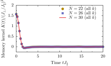
The typicality relation in Eqs. (S11), (S12), and (S13) can be calculated for as many sites as $N=30$, using a fourth-order Runge-Kutta iterator with a discrete time step $\delta tJ_{\parallel}=0.01\ll 1$ and sparse-matrix representations of the operators $H_{\parallel}$ and $j^{\prime}$ Ssteinigeweg2014-2 . In Fig. S1 we depict our results on the time dependence of $K(t)$ for $\beta\to 0$ and different $N$. Apparently, $K(t)$ does not depend on $N$ and fully decays on a rather short time scale $\tau_{K}\,J_{\parallel}\sim 2$. Thus, the Markov approximation is indeed justified. Note that the area under the $K(t)$ curve is the scattering rate $\gamma$ shown in Fig. 4 (b) of our Letter.

Figure S1: (Color online) Full time dependence of the memory kernel $K(t)$, according to the leading-order prediction in Eq. (S3), for high temperatures $\beta\to 0$ and different lattice sites $N=22$, $26$, $30$. The data depicted is numerically calculated using the typicality relation in Eqs. (S11), (S12), (S13) and a fourth-order Runge-Kutta iterator with a discrete time step $\delta t\,J_{\parallel}=0.01\ll 1$. Apparently, $K(t)$ does not depend on $N$ and fully decays on a rather short time scale $\tau_{K}\,J_{\parallel}\sim 2$. As compared to exact diagonalization of, say, $N=16$ sites, the Hilbert-space dimension accessible is larger by a factor of ca. $16,000$.

III Error Analysis

III.1 Specific Realization of the Initial State

Figure S2: (Color online) Error analysis: The time-dependent energy-current autocorrelation function $C(t)$ is numerically calculated according to the typicality relation in Eq. (4) of our Letter for two random initial states $|\psi\rangle_{1}\neq|\psi\rangle_{2}$, $N=30$ lattice sites, equal exchange couplings $J_{\perp}=J_{\parallel}$, and different temperatures (a) $\beta\,J_{\parallel}=0$, (b) $\beta\,J_{\parallel}=0.5$, (c) $\beta\,J_{\parallel}=1$. In addition, results for $N=32$ and a single initial state are shown. All results in (a)-(c) correspond to the sector $S^{z}=0$ and $k=0$. Insets: Relative deviation of the initial value $C(0)$, as obtained from $|\psi\rangle_{2}$ or $N=32$, from the $C(0)$ of $|\psi\rangle_{1}$. (Note that the $x$ axis is meaningless.) For the $\beta$ range depicted, the initial-state dependence is much below $1\%$ and smaller than the, also small, finite-size effects.

Our main numerical method used is essentially based on the typicality relation in Eq. (4) of our Letter, where the random error $\epsilon$ occurs. In this section we discuss this error in detail. The probability distribution $p(\epsilon)$, i.e., the probability to get an error of size $\epsilon$, has the mean

$$\bar{\epsilon}=0\,.$$ (S14)

Hence, if averaging is performed over sufficiently many random initial states $|\psi\rangle_{i}$, then any error vanishes. Note that we do not need to perform such averaging for reasons outlined below. The width of the probability distribution $p(\epsilon)$ is upper bounded by Selsayed2013 ; Ssteinigeweg2014-1 ; Ssteinigeweg2014-2

$$\sigma(\epsilon)\leq{\cal O}\left(\frac{\sqrt{\text{Re}\,\langle j(t)\,j\,j(t)\,j\rangle}}{N\,\sqrt{d_{\text{eff}}}}\right)\,,$$ (S15)

where the effective dimension

$$d_{\text{eff}}=\text{Tr}\{e^{-\beta(H-E_{0})}\}$$ (S16)

is the partition function and $E_{0}$ denotes the ground-state energy. Hence, the maximum error $\sigma(\epsilon)$ decreases faster with system size than $1/\sqrt{d_{\text{eff}}}$ does. In the limit of high temperatures, $\beta\to 0$, $d_{\text{eff}}=2^{N}$ is a huge number for $N\sim 30$ and the maximum error consequently is tiny. In fact, it has been shown in Ref. Ssteinigeweg2014-2, that significant errors only occur for effective dimensions below $d_{\text{eff}}\sim 10,000$, e.g., for rather small $N$. However, for large $N$, $d_{\text{eff}}$ can also become small for two reasons relevant to the study in our Letter.

(i) To reduce computational effort for large $N\geq 30$, we restrict our investigation to a single but representative symmetry subspace, i.e., to the quantum numbers $S^{z}=0$ and $k=0$. While this restriction does not have impact on the exact autocorrelation function $C(t)$, the dimension of the subspace

$$d_{0,0}\approx\frac{1}{N/2}\binom{N}{N/2}\ll 2^{N}$$ (S17)

is much smaller than the full Hilbert-space dimension. In the high-temperature limit, $\beta\to 0$, $d_{\text{eff}}=d_{0,0}$ is still a large number for $N\sim 30$.

(ii) If temperature is reduced from infinity at fixed $N$, $d_{\text{eff}}$ gradually deceases and eventually becomes $1$ at zero temperature. Therefore, $d_{\text{eff}}$ becomes a small number for sufficiently low temperatures and, as a consequence, the upper bound in Eq. (S15) does not imply a small $\epsilon$ any further. Note that $\epsilon$ can still be small since $\epsilon=0$ at zero temperature.

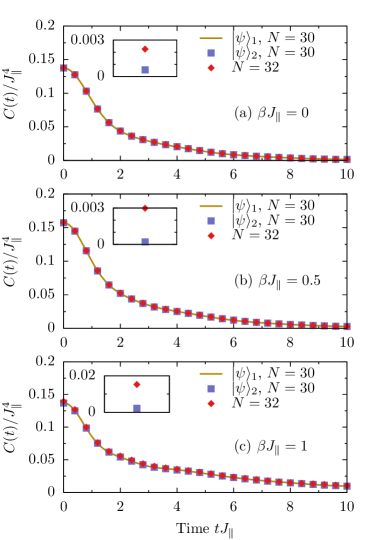
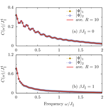
Due to (i) and (ii), it is important to verify in praxis that $\epsilon$ is indeed a negligibly small error. This verification is most conveniently done by repeating the calculation of the autocorrelation function $C(t)$ for a second random initial state $|\psi\rangle_{2}\neq|\psi\rangle_{1}$. In Fig. S2 we depict $C(t)$, as obtained from $|\psi\rangle_{1}$ and $|\psi\rangle_{2}$, for $N=30$ lattice sites, quantum numbers $S^{z}=0$ and $k=0$, equal couplings $J_{\perp}=J_{\parallel}$, and different temperatures $\beta\,J_{\parallel}\leq 1$. For this temperature range, we extract the heat conductivity in our Letter. Clearly, the $C(t)$ curves for $|\psi\rangle_{1}$ and $|\psi\rangle_{2}$ in Fig. S2 are very close to each other. This independence of the specific realization of the random initial state proves a small $\epsilon$ for temperatures $\beta\,J_{\parallel}=1$.

It is also instructive to quantify the size of errors. To this end, let us consider the relative error of the initial value given by

$$\epsilon_{r}(0)=\frac{|C(0,|\psi\rangle_{2})-C(0,|\psi\rangle_{1})|}{C(0,|\psi\rangle_{1})}\,.$$ (S18)

As shown in the insets of Fig. S2, $\epsilon_{r}(0)$ is much smaller than $1\%$ and particularly smaller than the, also small, finite-size effects.

Figure S3: (Color online) Error analysis: Real-time dependence of (a) energy-current autocorrelation function $C(t)$ and (b) norm $\sqrt{\langle\Phi_{\beta}(t)|\Phi_{\beta}(t)\rangle}$ of the pure state $|\Phi_{\beta}(t)\rangle$ in Eq. (4) of our Letter for small inter-chain coupling $J_{\perp}/J_{\parallel}=0.1$, $N=30$ lattice sites, sector $S^{z}=0$ and $k=0$, and high temperatures $\beta\to 0$. Although $C(t)$ decays on a long time scale, the norm $\sqrt{\langle\Phi_{\beta}(t)|\Phi_{\beta}(t)\rangle}$ does not deviate more than $0.25\%$ from $1$ on this time scale. Hence, our choice of the Runge-Kutta time step $\delta t\,J_{\parallel}=0.01\ll 1$ is reasonable.

III.2 Runge-Kutta Time Step

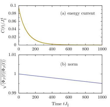
The typicality relation in Eq. (4) of our Letter requires to propagate pure states in real and imaginary time. We perform the propagation by a fourth-order Runge-Kutta iterator with a discrete time step $\delta t\,J_{\parallel}=0.01\ll 1$. This time step is a potential source for errors if the relaxation time of the energy current is very long, i.e., for very small inter-chain couplings $J_{\perp}/J_{\parallel}\ll 1$. To ensure sufficiently high accuracy, we verified for all $J_{\perp}$ that the norm of the two pure states $|\Phi_{\beta}(t)\rangle$ and $|\phi_{\beta}(t)\rangle$ propagated does not deviate significantly from $1$ on times up to the relaxation time of the energy current. In Fig. S2 we illustrate that, even for the demanding case $J_{\perp}/J_{\parallel}=0.1$, we find that deviations from $1$ are less than $1\%$. Note that reducing the time step for the large $N=30$ depicted is unfeasible for $J_{\perp}/J_{\parallel}\sim 0.1$.

Figure S4: (Color online) Error analysis: FTLM results for the frequency-dependent energy-current autocorrelation function $C(\omega)$ for different Lanczos steps $M=50$, $100$, $150$, $200$ and two temperatures (a) $\beta\,J_{\parallel}=0$ and (b) $\beta\,J_{\parallel}=1$. All results depicted correspond to strong coupling $J_{\perp}/J_{\parallel}=1$, $N=22$ lattice sites, and the sector $S^{z}=0$ (all $k$).

Figure S5: (Color online) Error analysis: FTLM results for the frequency-dependent energy-current autocorrelation function $C(\omega)$ for two different random states $|\Phi\rangle_{1}\neq|\Phi\rangle_{2}$ ($R=1$), an average over several $|\Phi\rangle_{i}$ ($R=10$), and two temperatures (a) $\beta\,J_{\parallel}=0$ and (b) $\beta\,J_{\parallel}=1$. All results depicted correspond to strong coupling $J_{\perp}/J_{\parallel}=1$, $N=22$ lattice sites, and the sector $S^{z}=0$ (all $k$).

III.3 Lanczos-Related Errors

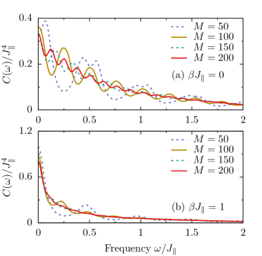
Within the Lanczos-diagonalization techniques used in our Letter, the origin of potential errors is twofold and related to Sprelovsek2013 : (i) spectral resolution $\delta\omega$ and (ii) number of effective terms in the thermodynamic sum $Z^{*}$.

(i) The spectral resolution is given by

$$\delta\omega=\frac{\Delta E}{M}\,,$$ (S19)

where $M$ is the number of Lanczos steps used. Note that we use $M=200$ for FTLM and $M=2000$ for MCLM in our Letter. $\Delta E=E_{\text{max}}-E_{\text{min}}$ is the full energy span of the Hamiltonian, i.e., $E_{\text{min}}$ and $E_{\text{max}}$ are the smallest and largest eigenenergy, respectively. This span depends only weakly on the inter-chain coupling $J_{\perp}$, e.g., for $N=22$ we find $\Delta E/J_{\parallel}\approx 30$ for the ladder case $J_{\perp}/J_{\parallel}=1$ and $\Delta E/J_{\parallel}\approx 20$ for the chain case $J_{\perp}/J_{\parallel}=0$. This span, together with $M=200$, yield $\delta\omega/J_{\parallel}\approx 0.15$. It is evident from Fig. 2 of our Letter that this spectral resolution is sufficient for large $J_{\perp}/J_{\parallel}={\cal O}(1)$. However, the spectrum $C(\omega)$ is narrow for small $J_{\perp}/J_{\parallel}=0.25$ and has a width of roughly $0.2\,J_{\parallel}$. Thus, we have to turn to MCLM and $M=2000$ for sufficiently high spectral resolution.

In Fig. S4 we show the $M$ dependence of the FTLM result for strong coupling $J_{\perp}/J_{\parallel}=1$, two temperatures $\beta\,J_{\parallel}=0$, $1$, and $N=22$ lattice sites. Obviously, finite $M$ are visible as quasi-periodic oscillations. But the overall structure of $C(\omega$) and the dc limit $C(\omega\to 0)$ are already well converged for $M=200$.

(b) Similar to the typicality approach discussed before, the statistical error of the Lanczos procedure is

$$\sigma(\epsilon)\leq{\cal O}\left(\frac{1}{\sqrt{RZ^{*}}}\right)\,,$$ (S20)

where $R$ is the number of random pure states used for sampling and $Z^{*}$ is the thermodynamic sum

$$Z^{*}=\sum_{n}e^{-\beta(E_{n}-E_{0})}\,,$$ (S21)

where $E_{0}$ is the ground-state energy. Note that, for $\beta=0$ and $\beta=\infty$, the thermodynamic sum $Z^{*}$ is equivalent to the effective dimension $d_{\text{eff}}$ in Eq. (S16). For any finite $\beta$, however, $Z^{*}\approx\text{d}_{\text{eff}}$ since energies $E_{n}$ located in the middle of the spectrum are approximately correct within the Lanczos technique. We find $Z^{*}\approx 450$ for $J_{\perp}/J_{\parallel}=1$, $N=22$, and $\beta\,J_{\parallel}=1$ and sample over $R=10$ random pure states for the $\beta\neq 0$ cases in Fig. 5 our Letter. For all $\beta=0$ cases, $R=1$.

In Fig. S5 we depict FTLM results for two different random states $|\Phi\rangle_{1}\neq|\Phi\rangle_{2}$ ($R=1$) and an average over several $|\Phi\rangle_{i}$ ($R=10$) for strong coupling $J_{\perp}/J_{\parallel}=1$, two temperatures $\beta\,J_{\parallel}=0$, $1$, and $N=22$ lattice sites. It is evident that the dependence on $R$ is negligibly small.

For a more detailed description of the implementation of FTLM and MCLM, we refer the interested reader to Refs. Sprelovsek2013, ; SJaklic1994, ; SLong2004, .

IV Equivalence of Ensembles

Figure S6: (Color online) The same as Fig. 2 (b) of our Letter but for the grand-canonical ensemble $\langle S^{z}\rangle=0$.

Figure S7: (Color online) (a) Real-time data underlying the $J_{\perp}/J_{\parallel}=1$ and $N=30$ DQT spectrum in Fig. S6. (b) The same as (a) but for $\beta J_{\parallel}=1\neq 0$. For comparison, in (a) and (b) the tDMRG data of Ref. Snote, is depicted.

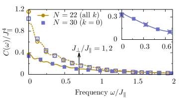
Finally, we also demonstrate that all results presented in our Letter do not depend on the restriction to the magnetization sector $S^{z}=0$ (canonical ensemble). To this end, we repeat the calculation in Fig. 2 (b) of our Letter for $\langle S^{z}\rangle=0$ (grand-canonical ensemble), taking into account all magnetization sectors. The result of this calculation is depicted in Fig. S6 and proves that $S^{z}=0$ and $\langle S^{z}\rangle=0$ yield the same physics.

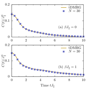
For the $J_{\parallel}/J_{\perp}=1$ and $N=30$ DQT spectrum shown in Fig. S6, we also depict in Fig. S7 (a) the underlying real-time data. Furthermore, we compare this real-time data to the tDMRG data of Ref. Snote, and find excellent agreement at $\beta J_{\parallel}=0$. As illustrated in Fig. S7 (b), the agreement between DQT and tDMRG data is also very good for $\beta J_{\parallel}=1$. Recall that the Fourier transforms in the inset of Fig. S6 rely on much longer times than those times depicted in Fig. S7.

Figure S8: (Color online) Real-time decay of the energy-current autocorrelation function $C(t)$ for $\beta J_{\parallel}=0,0.5,1$, obtained from DQT for $J_{\perp}/J_{\parallel}=0.5$ and $N=30$. (b) Spectrum for $\beta J_{\parallel}=1$, obtained by Fourier transforming data for finite times $t\leq 5\tau\sim 30/J_{\parallel}$. Inset: Temperature dependence of the conductivity $\kappa$, calculated by $N=30$ DQT. The overall figure is similar to Fig. 5 of our Letter, where $J_{\perp}/J_{\parallel}=1$.

V Temperature Dependence

To illustrate that the temperature dependence of the heat conductivity does not depend on the specific point $J_{\perp}/J_{\parallel}=1$ considered in our Letter, we also repeat the calculation in Fig. 5 for $J_{\perp}/J_{\parallel}=0.5$. The results of this calculation are shown in Fig. S8. Most importantly, we again find the scaling $\kappa\propto T^{-2}$ down to $T$ on the order of the exchange coupling, as shown in the inset of Fig. S8 (a).

References

- (1) D. C. Johnston et al., Phys. Rev. B 61, 9558 (2000).
- (2) J. M. Deutsch, Phys. Rev. A 43, 2046 (1991).
- (3) M. Srednicki, Phys. Rev. E 50, 888 (1994).
- (4) M. Rigol, V. Dunjko, and M. Olshanii, Nature 452, 854 (2008).
- (5) S. Trotzky et al., Science 319, 295 (2008).
- (6) P. Gambardella, Nature Mat. 5, 431 (2006).
- (7) M. Kruczenski, Phys. Rev. Lett. 93, 161602 (2004).
- (8) Y. B. Kim, Phys. Rev. B 53, 16420 (1996).
- (9) X. Zotos, F. Naef, and P. Prelovšek, Phys. Rev. B 55, 11029 (1997).
- (10) A. Klümper and K. Sakai, J. Phys. A: Math. Gen. 35, 2173 (2002).
- (11) A. V. Sologubenko et al., Phys. Rev. Lett. 84, 2714 (2000).
- (12) C. Hess et al., Phys. Rev. B 64, 184305 (2001).
- (13) C. Hess et al. Phys. Rev. Lett. 98, 027201 (2007).
- (14) N. Hlubek et al., Phys. Rev. B 81, 20405R (2010).
- (15) B. S. Shastry and B. Sutherland, Phys. Rev. Lett. 65, 243 (1990).
- (16) B. N. Narozhny, A. J. Millis, and N. Andrei, Phys. Rev. B 58, 2921R (1998).
- (17) X. Zotos, Phys. Rev. Lett. 82, 1764 (1999).
- (18) J. Benz et al., J. Phys. Soc. Jpn. 74, 181 (2005).
- (19) S. Fujimoto and N. Kawakami, Phys. Rev. Lett. 90, 197202 (2003).
- (20) T. Prosen, Phys. Rev. Lett. 106, 217206 (2011).
- (21) T. Prosen and E. Ilievski, Phys. Rev. Lett. 111, 057203 (2013).
- (22) J. Herbrych, P. Prelovšek, and X. Zotos, Phys. Rev. B 84, 155125 (2011).
- (23) C. Karrasch, J. H. Bardarson, and J. E. Moore, Phys. Rev. Lett. 108, 227206 (2012).
- (24) C. Karrasch et al., Phys. Rev. B 87, 245128 (2013).
- (25) R. Steinigeweg, J. Gemmer, and W. Brenig, Phys. Rev. Lett. 112, 120601 (2014).
- (26) R. Steinigeweg, J. Gemmer, and W. Brenig, Phys. Rev. B 91, 104404 (2015).
- (27) J. M. P. Carmelo, T. Prosen, and D. K. Campbell, preprint, arXiv:1407.0732 (2014).
- (28) J. Sirker, R. G. Pereira, and I. Affleck, Phys. Rev. Lett. 103, 216602 (2009).
- (29) J. Sirker, R. G. Pereira, and I. Affleck, Phys. Rev. B 83, 035115 (2011).
- (30) S. Grossjohann and W. Brenig, Phys. Rev. B 81, 012404 (2010).
- (31) M. Žnidarič, Phys. Rev. Lett. 106, 220601 (2011).
- (32) R. Steinigeweg and W. Brenig, Phys. Rev. Lett. 107, 250602 (2011).
- (33) C. Karrasch, J. E. Moore, and F. Heidrich-Meisner, Phys. Rev. B 89, 075139 (2014).
- (34) K. R. Thurber et al., Phys. Rev. Lett 87, 247202 (2001).
- (35) H. Maeter et al., J. Phys.: Condens. Matter 25, 365601 (2013).
- (36) J. P. Ronzheimer et al., Phys. Rev. Lett. 110, 205301 (2013).
- (37) S. Hild et al., Phys. Rev. Lett. 113, 147205 (2014).
- (38) F. Xiao et al., preprint, arXiv:1406.3202 (2014).
- (39) E. Shimshoni, N. Andrei, and A. Rosch, Phys. Rev. B 72, 059903 (2005).
- (40) A. V. Rozhkov and A. L. Chernyshev, Phys. Rev. Lett. 94, 087201 (2005).
- (41) N. Hlubek et al., J. Stat. Mech. 12, P03006 (2012).
- (42) Y. Huang, C. Karrasch, J. E. Moore, Phys. Rev. B 88, 115126 (2013).
- (43) C. Karrasch, R. Ilan, and J. E. Moore, Phys. Rev. B 88, 195129 (2013).
- (44) A. Karahalios et al., Phys. Rev. B 79, 024425 (2009).
- (45) F. Heidrich-Meisner et al., Phys. Rev. B 68, 134436 (2003).
- (46) R. Steinigeweg, J. Herbrych, P. Prelovšek, Phys. Rev. E 87, 012118 (2013).
- (47) E. Dagotto and T. M. Rice, Science 271, 618 (1996).
- (48) B. Lake et al., Nature Phys. 6, 50 (2010).
- (49) S. Notbohm et al., Phys. Rev. Lett. 98, 027403 (2007).
- (50) D. Schmidiger et al., Phys. Rev. B 88, 094411 (2013).
- (51) B. Thielemann et al., Phys. Rev. Lett. 102, 107204 (2009).
- (52) B. Thielemann et al., Phys. Rev. B 79, 020408 (2009).
- (53) G. B. Martins, M. Laukamp, J. Riera, and E. Dagotto, Phys. Rev. Lett. 78, 3563 (1997).
- (54) J. M. Tranquad et al., Nature 429, 534 (2004).
- (55) E. Dagotto, J. Riera, and D. Scalapino, Phys. Rev. B 45, 5744(R) (1992).
- (56) J. J. García-Ripoll, M. A. Martin-Delgado, and J. I. Cirac, Phys. Rev. Lett. 93, 250405 (2004).
- (57) Y. Li et al., Phys. Rev. A 71, 022301 (2005).
- (58) V. V. Deshpande et al., Science 323, 106 (2009).
- (59) P. Jung, R. W. Helmes, and A. Rosch, Phys. Rev. Lett. 96, 067202 (2006).
- (60) P. Jung and A. Rosch, Phys. Rev. B 76, 245108 (2007).
- (61) X. Zotos, Phys. Rev. Lett. 92, 067202 (2004).
- (62) C. Karrasch, D. M. Kennes, and F. Heidrich-Meisner, Phys. Rev. B 91, 115130 (2015).
- (63) R. Steinigeweg et al., Phys. Rev. B 90, 094417 (2014).
- (64) T. A. Elsayed and B. V. Fine, Phys. Rev. Lett. 110, 070404 (2013).
- (65) J. Gemmer and G. Mahler, Eur. Phys. J. B 31, 249 (2003).
- (66) S. Goldstein et al., Phys. Rev. Lett. 96, 050403 (2006).
- (67) S. Popescu, A. J. Short, and A. Winter, Nature Phys. 2, 754 (2006).
- (68) P. Reimann, Phys. Rev. Lett. 99, 160404 (2007).
- (69) S. R. White, Phys. Rev. Lett. 102, 190601 (2009).
- (70) C. Bartsch and J. Gemmer, Phys. Rev. Lett. 102, 110403 (2009).
- (71) C. Bartsch and J. Gemmer, EPL 96, 60008 (2011).
- (72) S. Sugiura and A. Shimizu, Phys. Rev. Lett. 108, 240401 (2012).
- (73) A. Hams and H. De Raedt, Phys. Rev. E 62, 4365 (2000).
- (74) R. Steinigeweg and R. Schnalle, Phys. Rev. E 82, 040103R (2010).
- (75) R. Steinigeweg, Phys. Rev. E 84, 011136 (2011).
- (76) A recent review is given in: P. Prelovšek and J. Bonča, Ground State and Finite Temperature Lanczos Methods in Strongly Correlated Systems, Solid-State Sciences 176 (Springer, Berlin, 2013).
- (77) See Supplemental Material.
- (1) P. Jung, R. W. Helmes, and A. Rosch, Phys. Rev. Lett. 96, 067202 (2006).
- (2) P. Jung and A. Rosch, Phys. Rev. B 76, 245108 (2007).
- (3) R. Steinigeweg and R. Schnalle, Phys. Rev. E 82, 040103R (2010).
- (4) R. Steinigeweg, Phys. Rev. E 84, 011136 (2011).
- (5) T. A. Elsayed and B. V. Fine, Phys. Rev. Lett. 110, 070404 (2013).
- (6) R. Steinigeweg, J. Gemmer, and W. Brenig, Phys. Rev. Lett. 112, 120601 (2014).
- (7) R. Steinigeweg, J. Gemmer, and W. Brenig, Phys. Rev. B 91, 104404 (2015).
- (8) P. Prelovšek and J. Bonča, Ground State and Finite Temperature Lanczos Methods in Strongly Correlated Systems, Solid-State Sciences 176 (Springer, Berlin, 2013).
- (9) J. Jaklič and P. Prelovšek, Phys. Rev. B 49, 5065(R) (1994).
- (10) M. W. Long, P. Prelovšek, S. El Shawish, J. Karadamoglou, and X. Zotos, Phys. Rev. B 70, 205129 (2004).
- (11) C. Karrasch, D. M. Kennes, and F. Heidrich-Meisner, Phys. Rev. B 91, 115130 (2015).