Heavy quark bound states in a quark-gluon plasma: dissociation and recombination

Jean-Paul Blaizot Institut de Physique Théorique (IPhT), CNRS/URA2306, CEA Saclay, F-91191 Gif-sur-Yvette, France Davide De Boni Department of Physics, Swansea University, Swansea SA2 8PP, Wales, United Kingdom Pietro Faccioli, Giovanni Garberoglio Dipartimento di Fisica Universitá degli Studi di Trento and
Trento Institute for Fundamental Physics and Applications (INFN-TIFPA),
Via Sommarive 14, Povo (Trento) 38123, Italy
Abstract

We present a comprehensive approach to the dynamics of heavy quarks in a quark gluon plasma, including the possibility of bound state formation and dissociation. In this exploratory paper, we restrict ourselves to the case of an Abelian plasma, but the extension of the techniques used to the non Abelian case is straightforward. A chain of well defined approximations leads eventually to a generalized Langevin equation, where the force and the noise terms are determined from a correlation function of the equilibrium plasma, and depend explicitly on the configuration of the heavy quarks. We solve the Langevin equation for various initial conditions, various numbers of heavy quark-antiquark pairs, and various temperatures of the plasma. Results of simulations illustrate various expected phenomena: dissociation of bound states as a result of combined effects of screening of the potential and collisions with the plasma constituent, formation of bound pairs (recombination) that occurs when enough heavy quarks are present in the system.

keywords:
Heavy Quarks, Quark-Gluon Plasma

1 Introduction

Heavy quarks produced in ultra-relativistic heavy ion collisions are interesting for a variety of reasons. They are created through hard processes taking place in small space time regions, at the very beginning of the collisions, and their abundances remain essentially frozen for the entire duration of the collisions. Thus heavy quarks can be used to diagnose the properties of the matter they cross before hadronizing. Heavy quarks can make bound states, such as the J/Ψ𝐽ΨJ/\Psi or the ΥΥ\Upsilon mesons, and the formation of such bound states can be strongly affected by the presence of a high temperature quark-gluon plasma. If the temperature of such a plasma is high enough, the binding forces can be screened at very short distance, hindering bound state formation, as was originally advocated in [1]. It was also argued that the presence of hot matter in the vicinity of a J/Ψ𝐽ΨJ/\Psi meson could produce an observable mass shift [2]. Note that other mechanisms, besides screening, involving in particular the collisions with the plasma constituents, can lead to bound state dissociation. This is so for instance of the analog of photo-dissociation, namely gluo-dissociation [3, 4, 5] (see also [6] for a recent study).

In situations where heavy quarks are abundantly produced, an excess of bound states could occur, due for instance to an enhanced recombination of cc¯𝑐¯𝑐c\bar{c} pairs into J/Ψ𝐽ΨJ/\Psi mesons at hadronization. Such a possibility was pointed out early on in Ref. [7] (see also[8]). Amusingly, the concern at that time was that the recombination mechanism could spoil the proposed signature of quark-gluon plasma, by hiding the expected J/Ψ𝐽ΨJ/\Psi suppression. Recombination was studied systematically using kinetic equations, viewing bound state formation and dissociation as a chemical reaction [9, 10]. A more extreme point of view is that bound states never truly form in a plasma (we shall come back to this important point shortly), but only when matter hadronizes, recombination being then treated as a statistical process [11] (see also [12] and [13]). Note that, in contrast to the initial worries, evidence for recombination would indicate that heavy quarks roam over long distances through the quark gluon plasma before recombining, thereby revealing a rather direct picture of a deconfined medium.

It turns out that the predicted phenomenon of J/Ψ𝐽ΨJ/\Psi suppression was observed experimentally in the first heavy ion collisions at the SPS, and later at RHIC (the reviews [14, 15] include a discussion of experimental results from SPS to RHIC). More recently, evidence was obtained at the LHC for sequential dissociation of the ΥΥ\Upsilon bound states, with the less bound states being more suppressed than the most tightly bound ones [16]. Some evidence for recombination was also presented by the ALICE experiment [17]. The interpretation of the data remains as of today uncertain for a variety of reasons, most of which having to do with the production mechanism of the heavy quark bound states (involving issues related to structure functions, shadowing, etc), the heavy ion reaction dynamics, etc, all aspects that are beyond the scope of the present paper. However, the quality of the recent data, and the potential of upcoming experiments, provide strong motivation for further theoretical efforts.

Many investigations concern the fate of the QQ¯𝑄¯𝑄Q\bar{Q} bound state immersed in a quark gluon plasma in equilibrium at some temperature T𝑇T. Such studies where initiated in [18] with the determination of the stationary states of a Schrödinger equation, with a temperature dependent potential that accounts for screening and the disappearance of the string tension at high temperature. There has been discussion on the ambiguity in the choice of the appropriate potential (free energy versus internal energy) and how to relate it to quantities calculable on the lattice. A review of such potential models can be found in [19]. A somewhat similar line of research concerns the calculation of the spectral functions of charmonium states on the lattice. While such calculations have the virtue of being first principle calculations within Quantum Chromodynamics (QCD), they suffer from a large uncertainty in the reconstruction of the spectral function through the maximum entropy technique (for a recent review of lattice calculation at finite temperature, including a discussion of this issue, see e.g. [20]). Going somewhat beyond the Schrödinger picture, the in-medium T-matrix approach [21] can encompass many effects beyond the screening of the potential; it can in principle deal with dissociation reactions, changes in thresholds related to shifts of masses, coupled channels, etc.

A recent progress in the direction of a more complete dynamical approach based on first principles was initiated in [22]. There one calculates a correlator that is directly related to an observable, the rate of dilepton production, and derive the Schrödinger equation obeyed by this correlator. A remarkable feature of this equation is that the potential that enters it has an imaginary part that reflects the effects of the collisions that the heavy quarks suffer with the plasma constituents. The origin of this complex potential was further studied in [23], and also in the context of the non relativistic heavy quark effective theory in [24, 25].

However, an important issue rarely addressed in the approaches that we have mentioned is that the process of the bound state formation is not instantaneous: heavy quarks start to interact with the plasma while the correlations that could eventually lead to a bound state build up (see e.g. [26] or [27] for early discussions of this issue). This is an important feature that should be taken into account when trying to get a complete dynamical picture. In short, it is clear that the heavy quarks will suffer collisions with the constituents of the surrounding plasma as soon as they are created, and the real issue is whether they will still form a bound state when the plasma has cooled down, not whether the bound state will “survive”.

The goal of the present paper is to address this and other issues, by developing a comprehensive approach of the entire dynamics of the heavy quarks, including the possibilities for bound state formation and dissociation. We shall do that trying to stay as close as possible to first principles, and using a chain of well defined (in some cases well controlled) approximations. The main objective is to get a global view of the dynamics of heavy quarks. As we proceed we shall recover some of the many pieces that have been addressed separately in some of the works mentioned above. The approach builds up, extends, and to some extent completes, previous works by some of the authors [23, 28]. It is similar in spirit to analogous recent efforts using the language of open quantum system [29, 30, 31] (see also [32, 33]). We shall be led eventually to formulate, at the end of our approximation chain, a generalized Langevin equation, and in that respect, our work bears similarities with previous studies using Langevin dynamics for heavy quarks [34, 35, 36]. The present work goes beyond such studies by taking into account the dependence of the noise term on the configuration of the heavy quarks at each time step. This is an important aspect of the dynamics, but it makes the Langevin equation more difficult to solve. In devising suitable techniques to handle it, we were inspired by similar problems in other fields of physics, in particular by techniques used in soft matter physics [37].

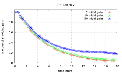
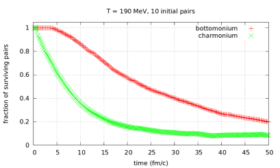
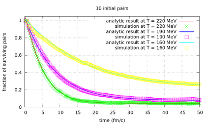
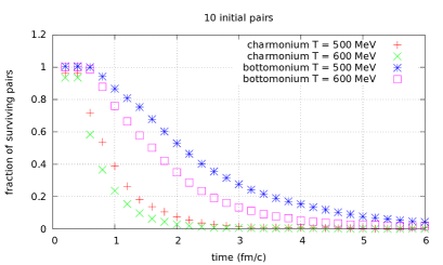
In this exploratory work we focus on the general issue of the formation of bound sates of heavy particles in a thermal bath of light particles. The paper is organized as follows. In the next section we summarize the general formalism that we are using. We treat the heavy particles as non relativistic, and the plasma particles as relativistic. We ignore the specifics of QCD interactions, and for instance the change of their nature (from attractive to repulsive) depending on the color state (singlet or octet) the quark-antiquark pairs are in. Only Coulomb interactions are retained. The goal of this section is to write the probability for a collection of quarks started at some positions at initial time to be found at a later time at some other positions. This is formulated in terms of a path integral from which we derive an effective theory for the heavy quarks, usually referred to in such a context as the “influence functional”. The main approximation in the elimination of the plasma degrees of freedom is a weak coupling ansatz that allows us to ignore non linear interactions among the gluons. With this approximation, the effective action for the heavy quarks takes the simple form of an action quadratic in the charge density of the heavy quarks. The whole information about the plasma is contained in a 2-point function. The content of the functional is analyzed in section 3 where we study the infinite mass limit of a related object, the correlator of a heavy quark-antiquark pair. In this case, the plasma 2-point function reduces to a complex potential whose real part describes the screening phenomenon, while the imaginary part takes into account the effects of the collisions. The infinite mass limit is the leading order of a systematic approximation, the low frequency approximation, that we use to calculate the influence functional in the following section. The low frequency approximation exploits the fact that the mass of the heavy quark is large, and can be viewed as an expansion in terms of the velocity of the heavy particles. The leading terms yield a generalized Langevin equation with a multiplicative (position dependent) noise. The ingredients of the Langevin equation are related to the real and imaginary part of the potential. In Sect. 5 we present results of a set of simulations that we have carried out for the case of 2, 10 or 50 pairs of particles. The various aspects of heavy quark propagation in a quark gluon plasma are illustrated, including the competing phenomena of dissociation and recombination. The last section contains a brief summary.

2 General setup

The general problem that we are addressing is that of the dynamics of a collection of heavy charged particles in a thermalized bath of light particles with which they interact. Although our ultimate goal is to treat QCD interactions, in this exploratory paper we focus on the case of Abelian interactions, that is, strictly speaking our picture applies directly to electromagnetic interactions. Still we shall use the language of QCD, and call the heavy charged particles quarks (with positive unit charge) or antiquarks (with negative unit charge). Similarly the plasma in which the heavy particles move will consist of massless charged particles, referred to as light quarks, and the photons they exchange will be called gluons. We hope this abuse of language will not cause confusion. It is motivated by the fact that the simulations that we shall present in this paper involve parameters that are adjusted so as to lead to orders of magnitude that are comparable to what we expect for heavy quarks in a quark-gluon plasma (in particular we use the strong coupling constant αs0.3subscript𝛼𝑠0.3\alpha_{s}\approx 0.3, not the electromagnetic one α1/137𝛼1137\alpha\approx 1/137). Most of the effects that we want to study would occur already in Abelian plasmas. Specific effects due to non Abelian color interactions will be discussed in forthcoming publications.

In this section we outline the general formalism that we use. The present approach builds on, and extends, that developed by some of us in Refs. [23, 28], and the notation used here is close to that of these papers. A related effort was undertaken recently in Refs. [29, 30, 31] which directly address the case of non Abelian plasmas. Our goal is to obtain an effective theory for the heavy quarks, by eliminating the plasma degrees of freedom. This will be achieved by exploiting the fact that the heavy quarks behave as non relativistic particles, whose number is conserved as they interact with the quark-gluon plasma, and whose mass is large compared to the scales that characterize the plasma dynamics. Ultimately, the plasma properties will enter the effective theory only through specific correlation functions that are, in leading order, simply related to the potential whose real part describes the screening phonemenon, and the imaginary part the effects of collisions.

The heavy quarks, as we just mentioned, are treated as massive non relativistic particles. When they thermalize, their typical wavelength, λ1/MTsimilar-to𝜆1𝑀𝑇\lambda\sim 1/\sqrt{MT} with M𝑀M is the mass and T𝑇T the temperature, is small compared to the inter particle distance of the plasma particles, 1/T1𝑇1/T. This suggests that the dynamics of the heavy particles is to a large extent classical, and indeed the approximation scheme that we shall present will lead us to a semi-classical description. The heavy particles interact among themselves, and with the charged plasma constituents via Coulomb interactions. We neglect magnetic interactions, which are suppressed by powers of the velocity, or the inverse mass of the heavy particles. Such restriction do not apply a priori to the light particles, but since heavy quarks will not excite magnetic modes, we ignore these altogether. Thus the plasma is modeled by massless quarks and antiquarks, interacting also with Coulomb interactions. As we shall see, the dynamics of the plasma is then characterized by a unique energy scale which is the screening mass mDsubscript𝑚𝐷m_{D}. In order to get sensible orders of magnitude later in our simulations, we choose this to be given by its perturbative value for a two flavor quark-gluon plasma, i.e., mD2=(4/3)g2T2superscriptsubscript𝑚𝐷243superscript𝑔2superscript𝑇2m_{D}^{2}=(4/3)g^{2}T^{2} where g𝑔g is the gauge coupling. We shall assume throughout this paper that mD<TMsubscript𝑚𝐷𝑇much-less-than𝑀m_{D}<T\ll M\,.

In Coulomb gauge 𝑨=0bold-∇𝑨0{\boldsymbol{\nabla}}\cdot{\boldsymbol{A}}=0, the Hamiltonian of the system reads

H𝐻\displaystyle H =\displaystyle= 12Mj=1N(𝐩j2+𝐩¯j2)+d𝒙ψ(𝒙)(𝜶i+mγ0)ψ(𝒙)+12𝑀superscriptsubscript𝑗1𝑁superscriptsubscript𝐩𝑗2superscriptsubscript¯𝐩𝑗2limit-fromdifferential-d𝒙superscript𝜓𝒙𝜶bold-∇𝑖𝑚subscript𝛾0𝜓𝒙\displaystyle\frac{1}{2M}\sum_{j=1}^{N}\left({\mathbf{p}}_{j}^{2}+\bar{\mathbf{p}}_{j}^{2}\right)+\int\mathop{}\!\mathrm{d}{{\boldsymbol{x}}}\leavevmode\nobreak\ {\psi}^{\dagger}({\boldsymbol{x}})\leavevmode\nobreak\ \left(\frac{{\boldsymbol{\alpha}}\cdot{\boldsymbol{\nabla}}}{i}+m\gamma_{0}\right)\leavevmode\nobreak\ \psi({\boldsymbol{x}})+ (2.1)
+\displaystyle+ 12d𝒙d𝒚ρtot(𝒙)K(𝒙𝒚)ρtot(𝒚),12differential-d𝒙differential-d𝒚subscript𝜌tot𝒙𝐾𝒙𝒚subscript𝜌tot𝒚\displaystyle\frac{1}{2}\int\!\!\!\!\>\int\mathop{}\!\mathrm{d}{{\boldsymbol{x}}}\mathop{}\!\mathrm{d}{{\boldsymbol{y}}}\leavevmode\nobreak\ \rho_{{}_{\scriptsize\mbox{tot}}}({\boldsymbol{x}})K({\boldsymbol{x}}-{\boldsymbol{y}})\rho_{{}_{\scriptsize\mbox{tot}}}({\boldsymbol{y}}),

where αi=γ0γisuperscript𝛼𝑖subscript𝛾0superscript𝛾𝑖\alpha^{i}=\gamma_{0}\gamma^{i} is a Dirac matrix, and ρtot=ρ+ρψsubscript𝜌tot𝜌subscript𝜌𝜓\rho_{{}_{\scriptsize\mbox{tot}}}=\rho+\rho_{\psi} is the total charge density, with

ρ(𝒙)=gj=1N[δ(𝒙𝒒j)δ(𝒙𝒒¯j)],𝜌𝒙𝑔superscriptsubscript𝑗1𝑁delimited-[]𝛿𝒙subscript𝒒𝑗𝛿𝒙subscript¯𝒒𝑗\displaystyle\rho({\boldsymbol{x}})=g\,\sum_{j=1}^{N}\left[\delta({\boldsymbol{x}}-{\bm{q}}_{j})-\delta({\boldsymbol{x}}-\bar{\bm{q}}_{j})\right], (2.2)

the charge density of the heavy quarks and antiquarks, and

ρψ(𝒙)=gψ(𝒙)ψ(𝒙)subscript𝜌𝜓𝒙𝑔superscript𝜓𝒙𝜓𝒙\displaystyle\rho_{\psi}({\boldsymbol{x}})=g\,\psi^{\dagger}({\boldsymbol{x}})\psi({\boldsymbol{x}}) (2.3)

the density of the charged plasma particles (here, charged light quarks and anitquarks). The plasma is supposed to be electrically neutral, that is, it contains the same number of light quarks and antiquarks. It is useful to rewrite the Hamiltonian (2.1) by separating its various contributions as follows

H=HQ+H1+Hpl,𝐻subscript𝐻𝑄subscript𝐻1subscript𝐻pl\displaystyle H=H_{Q}+H_{1}+H_{\rm pl}, (2.4)

with HQsubscript𝐻𝑄H_{Q} describing the dynamics of the heavy quarks in the absence of the plasma,

HQ=12Mj=1N(𝐩j2+𝐩¯j2)+12d𝒙d𝒚ρ(𝒙)K(𝒙𝒚)ρ(𝒚),subscript𝐻𝑄12𝑀superscriptsubscript𝑗1𝑁superscriptsubscript𝐩𝑗2superscriptsubscript¯𝐩𝑗212differential-d𝒙differential-d𝒚𝜌𝒙𝐾𝒙𝒚𝜌𝒚\displaystyle H_{Q}=\frac{1}{2M}\sum_{j=1}^{N}\left({\mathbf{p}}_{j}^{2}+\bar{\mathbf{p}}_{j}^{2}\right)+\frac{1}{2}\int\!\!\!\!\>\int\mathop{}\!\mathrm{d}{{\boldsymbol{x}}}\mathop{}\!\mathrm{d}{{\boldsymbol{y}}}\,\rho({\boldsymbol{x}})K({\boldsymbol{x}}-{\boldsymbol{y}})\rho({\boldsymbol{y}}), (2.5)

H1subscript𝐻1H_{1} the Hamiltonian coupling the heavy quarks to the plasma charged particles

H1=d𝒙d𝒚ρ(𝒙)K(𝒙𝒚)ρψ(𝒚),subscript𝐻1differential-d𝒙differential-d𝒚𝜌𝒙𝐾𝒙𝒚subscript𝜌𝜓𝒚\displaystyle H_{1}=\int\!\!\!\!\>\int\mathop{}\!\mathrm{d}{{\boldsymbol{x}}}\mathop{}\!\mathrm{d}{{\boldsymbol{y}}}\,\rho({\boldsymbol{x}})K({\boldsymbol{x}}-{\boldsymbol{y}})\rho_{\psi}({\boldsymbol{y}}), (2.6)

and Hplsubscript𝐻plH_{\rm pl} the Hamiltonian of the plasma in the absence of the heavy quarks

Hpl=d𝒙ψ(𝒙)(𝜶i+mγ0)ψ(𝒙)+12d𝒙d𝒚ρψ(𝒙)K(𝒙𝒚)ρψ(𝒚),subscript𝐻pldifferential-d𝒙superscript𝜓𝒙𝜶bold-∇𝑖𝑚subscript𝛾0𝜓𝒙12differential-d𝒙differential-d𝒚subscript𝜌𝜓𝒙𝐾𝒙𝒚subscript𝜌𝜓𝒚\displaystyle H_{\rm pl}=\int\mathop{}\!\mathrm{d}{{\boldsymbol{x}}}\,{\psi}^{\dagger}({\boldsymbol{x}})\left(\frac{{\boldsymbol{\alpha}}\cdot{\boldsymbol{\nabla}}}{i}+m\gamma_{0}\right)\psi({\boldsymbol{x}})+\frac{1}{2}\int\!\!\!\!\>\int\mathop{}\!\mathrm{d}{{\boldsymbol{x}}}\mathop{}\!\mathrm{d}{{\boldsymbol{y}}}\,\rho_{\psi}({\boldsymbol{x}})K({\boldsymbol{x}}-{\boldsymbol{y}})\rho_{\psi}({\boldsymbol{y}}), (2.7)

We represent the heavy particles in first quantization (they are non relativistic particles whose number is conserved), while the light particles are represented by the fermion fields ψ(𝒙)𝜓𝒙\psi({\boldsymbol{x}}) and ψ(𝒙)superscript𝜓𝒙\psi^{\dagger}({\boldsymbol{x}}). Note that the interaction term in Eq. (2.5) contains contributions of self interactions. Such terms will not contribute in the final equations that enter our simulations111They play a role in the real part of the potential to be discussed in Sect. 3.. We call 𝒒jsubscript𝒒𝑗{\bm{q}}_{j} and 𝒒¯jsubscript¯𝒒𝑗\bar{\bm{q}}_{j}, with j=1,,N𝑗1𝑁j=1,\cdots,N, the coordinates of, respectively, the heavy quarks and antiquarks, and 𝒑jsubscript𝒑𝑗{\bm{p}}_{j}, 𝒑¯jsubscript¯𝒑𝑗\bar{\bm{p}}_{j} the corresponding momenta. We denote collectively these coordinates by a 2N2𝑁2N dimensional vector 𝑸=(𝒒1,,𝒒N,𝒒¯1,,𝒒¯N)𝑸subscript𝒒1subscript𝒒𝑁subscript¯𝒒1subscript¯𝒒𝑁{\boldsymbol{Q}}=\left({\bm{q}}_{1},\cdots,{\bm{q}}_{N},\bar{\bm{q}}_{1},\cdots,\bar{\bm{q}}_{N}\right)\,, and often refer to 𝑸𝑸{\boldsymbol{Q}} as a configuration. The last term in Eq. (2.1) is the total Coulomb energy, with

K(𝒙𝒚)=14π|𝒙𝒚|,x2K(xy)=δ(xy).formulae-sequence𝐾𝒙𝒚14𝜋𝒙𝒚subscriptsuperscriptbold-∇2𝑥𝐾𝑥𝑦𝛿𝑥𝑦\displaystyle K({\boldsymbol{x}}-{\boldsymbol{y}})=\frac{1}{4\pi|{\boldsymbol{x}}-{\boldsymbol{y}}|},\qquad-{\boldsymbol{\nabla}}^{2}_{x}K(x-y)=\delta(x-y). (2.8)

We are interested in the probability P(𝑸f,tf|𝑸i,ti)𝑃subscript𝑸𝑓conditionalsubscript𝑡𝑓subscript𝑸𝑖subscript𝑡𝑖P({\boldsymbol{Q}}_{f},t_{f}|{\boldsymbol{Q}}_{i},t_{i}) to find the heavy particles in a configuration 𝑸fsubscript𝑸𝑓{\boldsymbol{Q}}_{f} at time tfsubscript𝑡𝑓t_{f}, given that they are in a configuration 𝑸isubscript𝑸𝑖{\boldsymbol{Q}}_{i} at time tisubscript𝑡𝑖t_{i}. This probability may be written in terms of the density matrix of the entire system (the plasma and the heavy particles). Let 𝒟𝒟{\cal D} be this density matrix. At time tisubscript𝑡𝑖t_{i} we assume that the heavy quarks have not yet interacted with the plasma, so that the density matrix takes the factorized form 𝒟(0)=𝒟Q(i)𝒟pl(i)𝒟0tensor-productsuperscriptsubscript𝒟𝑄𝑖superscriptsubscript𝒟pl𝑖{\cal D}(0)={\cal D}_{Q}^{(i)}\otimes{\cal D}_{\rm pl}^{(i)}, with 𝒟Q(i)=|𝑸i𝑸i|superscriptsubscript𝒟𝑄𝑖ketsubscript𝑸𝑖brasubscript𝑸𝑖{\cal D}_{Q}^{(i)}=|{\boldsymbol{Q}}_{i}\rangle\langle{\boldsymbol{Q}}_{i}|, a projector on the configuration 𝑸isubscript𝑸𝑖{\boldsymbol{Q}}_{i}, and 𝒟pl(i)=1ZpleβHplsuperscriptsubscript𝒟pl𝑖1subscript𝑍plsuperscripte𝛽subscript𝐻pl{\cal D}_{\rm pl}^{(i)}=\frac{1}{Z_{\rm pl}}{\rm e}^{-\beta H_{\rm pl}} is the density matrix of the plasma in thermal equilibrium at temperature T=1/β𝑇1𝛽T=1/\beta, with Zpl=exp(βFpl)subscript𝑍pl𝛽subscript𝐹plZ_{\rm pl}=\exp(\beta F_{\rm pl}) the partition function of the plasma and Fplsubscript𝐹plF_{\rm pl} its free energy. The density matrix at time t𝑡t is given by 𝒟(t)=eiHt𝒟(0)eiHt𝒟𝑡superscripte𝑖𝐻𝑡𝒟0superscripte𝑖𝐻𝑡{\cal D}(t)={\rm e}^{-iHt}{\cal D}(0){\rm e}^{iHt}, and the looked for probability can be written in the form

P(𝑸f,tf|𝑸i,ti)𝑃subscript𝑸𝑓conditionalsubscript𝑡𝑓subscript𝑸𝑖subscript𝑡𝑖\displaystyle P({\boldsymbol{Q}}_{f},t_{f}|{\boldsymbol{Q}}_{i},t_{i}) =\displaystyle= Tr{[|𝑸f𝑸f|𝕀]𝒟(t)}Trdelimited-[]tensor-productketsubscript𝑸𝑓brasubscript𝑸𝑓𝕀𝒟𝑡\displaystyle{\rm Tr}\left\{\left[|{\boldsymbol{Q}}_{f}\rangle\langle{\boldsymbol{Q}}_{f}|\otimes{\mathbb{I}}\right]{\cal D}(t)\right\} (2.9)
=\displaystyle= n,meβEmplZpl𝑸i,m|eiHt|𝑸f,n𝑸f,n|eiHt|𝑸i,msubscript𝑛𝑚superscripte𝛽subscriptsuperscript𝐸pl𝑚subscript𝑍plquantum-operator-productsubscript𝑸𝑖𝑚superscripte𝑖𝐻𝑡subscript𝑸𝑓𝑛quantum-operator-productsubscript𝑸𝑓𝑛superscripte𝑖𝐻𝑡subscript𝑸𝑖𝑚\displaystyle\sum_{n,m}\frac{{\rm e}^{-\beta E^{\rm pl}_{m}}}{Z_{\rm pl}}\langle{\boldsymbol{Q}}_{i},m|{\rm e}^{iHt}|{\boldsymbol{Q}}_{f},n\rangle\langle{\boldsymbol{Q}}_{f},n|{\rm e}^{-iHt}|{\boldsymbol{Q}}_{i},m\rangle
=\displaystyle= n,meβEmplZpl|𝑸f,n|eiHt|𝑸i,m|2,subscript𝑛𝑚superscripte𝛽subscriptsuperscript𝐸pl𝑚subscript𝑍plsuperscriptquantum-operator-productsubscript𝑸𝑓𝑛superscripte𝑖𝐻𝑡subscript𝑸𝑖𝑚2\displaystyle\sum_{n,m}\frac{{\rm e}^{-\beta E^{\rm pl}_{m}}}{Z_{\rm pl}}\left|\langle{\boldsymbol{Q}}_{f},n|{\rm e}^{-iHt}|{\boldsymbol{Q}}_{i},m\rangle\right|^{2},

where we have set ttfti𝑡subscript𝑡𝑓subscript𝑡𝑖t\equiv t_{f}-t_{i}. In order to trace out the degrees of freedom of the plasma, as implied by the formula above, it is convenient to rewrite this expression in terms of path integrals.

We shall do so in steps, in order to identify the main components of the formalism. Let us first consider the simple case where the heavy particles interact only with an external potential A0(𝒙)subscript𝐴0𝒙A_{0}({\boldsymbol{x}}), with a Hamiltonian H1=g𝒙ρ(𝒙)A0(𝒙)subscript𝐻1𝑔subscript𝒙𝜌𝒙subscript𝐴0𝒙H_{1}=g\int_{{\boldsymbol{x}}}\rho({\boldsymbol{x}})A_{0}({\boldsymbol{x}}). In this case222As we shall see shortly this case is relevant for the general discussion.

P(𝑸f,tf|𝑸i,ti)=|𝑸f,tf|𝑸i,ti|2.𝑃subscript𝑸𝑓conditionalsubscript𝑡𝑓subscript𝑸𝑖subscript𝑡𝑖superscriptinner-productsubscript𝑸𝑓subscript𝑡𝑓subscript𝑸𝑖subscript𝑡𝑖2\displaystyle P({\boldsymbol{Q}}_{f},t_{f}|{\boldsymbol{Q}}_{i},t_{i})=\left|\langle{\boldsymbol{Q}}_{f},t_{f}|{\boldsymbol{Q}}_{i},t_{i}\rangle\right|^{2}. (2.10)

and the probability amplitude 𝑸f,tf|𝑸i,tiinner-productsubscript𝑸𝑓subscript𝑡𝑓subscript𝑸𝑖subscript𝑡𝑖\langle{\boldsymbol{Q}}_{f},t_{f}|{\boldsymbol{Q}}_{i},t_{i}\rangle is given by a Feynman path integral

𝑸f,tf|𝑸i,tiinner-productsubscript𝑸𝑓subscript𝑡𝑓subscript𝑸𝑖subscript𝑡𝑖\displaystyle\langle{\boldsymbol{Q}}_{f},t_{f}|{\boldsymbol{Q}}_{i},t_{i}\rangle =\displaystyle= 𝑸i𝑸fD𝑸ei(S0[𝑸]+S1[𝑸,A0]),superscriptsubscriptsubscript𝑸𝑖subscript𝑸𝑓𝐷𝑸superscripte𝑖subscript𝑆0delimited-[]𝑸subscript𝑆1𝑸subscript𝐴0\displaystyle\int_{{\boldsymbol{Q}}_{i}}^{{\boldsymbol{Q}}_{f}}D{\boldsymbol{Q}}\;\mathrm{e}^{i(S_{0}[{\boldsymbol{Q}}]+S_{1}[{\boldsymbol{Q}},A_{0}])}, (2.11)

where the paths 𝑸(t)𝑸𝑡{\boldsymbol{Q}}(t) satisfy 𝑸(ti)=𝑸i𝑸subscript𝑡𝑖subscript𝑸𝑖{\boldsymbol{Q}}(t_{i})={\boldsymbol{Q}}_{i} and 𝑸(tf)=𝑸f𝑸subscript𝑡𝑓subscript𝑸𝑓{\boldsymbol{Q}}(t_{f})={\boldsymbol{Q}}_{f}. The actions S0subscript𝑆0S_{0} and S1subscript𝑆1S_{1} are given by

S0[𝑸]subscript𝑆0delimited-[]𝑸\displaystyle S_{0}[{\boldsymbol{Q}}] =\displaystyle= M2j=1Ntitfdt(𝒒˙j2+𝒒¯˙j2),𝑀2superscriptsubscript𝑗1𝑁superscriptsubscriptsubscript𝑡𝑖subscript𝑡𝑓differential-d𝑡subscriptsuperscript˙𝒒2𝑗subscriptsuperscript˙¯𝒒2𝑗\displaystyle\frac{M}{2}\sum_{j=1}^{N}\int_{t_{i}}^{t_{f}}{\rm d}t\left(\dot{\bm{q}}^{2}_{j}+\dot{\bar{\bm{q}}}^{2}_{j}\right), (2.12)
S1[𝑸,A0]subscript𝑆1𝑸subscript𝐴0\displaystyle S_{1}[{\boldsymbol{Q}},A_{0}] =\displaystyle= titfdtd3𝒙ρ(x)A0(x),superscriptsubscriptsubscript𝑡𝑖subscript𝑡𝑓differential-d𝑡superscriptd3𝒙𝜌𝑥subscript𝐴0𝑥\displaystyle-\int_{t_{i}}^{t_{f}}{\rm d}t\,\int{\rm d}^{3}{\boldsymbol{x}}\,\rho(x)A_{0}(x), (2.13)

where we have set x=(t,𝒙)𝑥𝑡𝒙x=(t,{\boldsymbol{x}}), and ρ(x)𝜌𝑥\rho(x) is the charge density of the heavy particles

ρ(x)=j=1Ng[δ(𝒙𝒒j(t)δ(𝒙𝒒¯j(t)],\displaystyle\rho(x)=\sum_{j=1}^{N}g\left[\delta({\boldsymbol{x}}-{\bm{q}}_{j}(t)-\delta({\boldsymbol{x}}-\bar{\bm{q}}_{j}(t)\right], (2.14)

so that S1subscript𝑆1S_{1} can also be written as

S1[𝑸,A0]=gj=1Ntitfdt[A0(𝒒j(t))A0(𝒒¯j(t))].subscript𝑆1𝑸subscript𝐴0𝑔superscriptsubscript𝑗1𝑁superscriptsubscriptsubscript𝑡𝑖subscript𝑡𝑓differential-d𝑡delimited-[]subscript𝐴0subscript𝒒𝑗𝑡subscript𝐴0subscript¯𝒒𝑗𝑡\displaystyle S_{1}[{\boldsymbol{Q}},A_{0}]=-g\sum_{j=1}^{N}\int_{t_{i}}^{t_{f}}\!\!\!{\rm d}t\,\left[A_{0}({\bm{q}}_{j}(t))-A_{0}(\bar{\bm{q}}_{j}(t))\right]. (2.15)

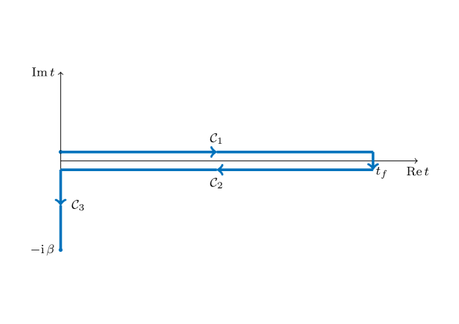
The probability (2.10) can be represented by a very similar formula, by using the closed-time path formalism. We introduce a contour in the complex time plane, as illustrated in Fig. 1, and consider the coordinates {𝒒i,𝒒¯i}subscript𝒒𝑖subscript¯𝒒𝑖\{{\bm{q}}_{i},\bar{\bm{q}}_{i}\} as functions of the complex time t𝒞subscript𝑡𝒞t_{\scriptsize{\cal C}} running along the contour. Alternatively, we may keep time real, but duplicate the coordinates, denoting by 𝑸1={𝒒i,1,𝒒¯i,1}subscript𝑸1subscript𝒒𝑖1subscript¯𝒒𝑖1{\boldsymbol{Q}}_{1}=\{{\bm{q}}_{i,1},\bar{\bm{q}}_{i,1}\} and 𝑸2={𝒒i,2,𝒒¯i,2}subscript𝑸2subscript𝒒𝑖2subscript¯𝒒𝑖2{\boldsymbol{Q}}_{2}=\{{\bm{q}}_{i,2},\bar{\bm{q}}_{i,2}\} the coordinates of the heavy particles living respectively on the upper branch (𝒞1subscript𝒞1{\cal C}_{1}, corresponding to the amplitude) and the lower branch (𝒞2subscript𝒞2{\cal C}_{2}, corresponding to the complex conjugate amplitude) of the contour. We can then write

P(𝑸f,tf|𝑸i,ti)=𝒞D𝑸ei(S0[𝑸]+S1[𝑸,A0]),𝑃subscript𝑸𝑓conditionalsubscript𝑡𝑓subscript𝑸𝑖subscript𝑡𝑖subscript𝒞𝐷𝑸superscripte𝑖subscript𝑆0delimited-[]𝑸subscript𝑆1𝑸subscript𝐴0\displaystyle P({\boldsymbol{Q}}_{f},t_{f}|{\boldsymbol{Q}}_{i},t_{i})=\int_{\cal C}D{\boldsymbol{Q}}\;\mathrm{e}^{i(S_{0}[{\boldsymbol{Q}}]+S_{1}[{\boldsymbol{Q}},A_{0}])}, (2.16)

where the actions S0subscript𝑆0S_{0} and S1subscript𝑆1S_{1} are given by the formulae (2.12,2.13) in which the time integrations are replaced by integrations along the Schwinger-Keldysh contour. Thus, for instance, S0subscript𝑆0S_{0} is given by

S0[𝑸]=M2j=1N𝒞dt𝒞(𝒒˙j2+𝒒¯˙j2),subscript𝑆0delimited-[]𝑸𝑀2superscriptsubscript𝑗1𝑁subscript𝒞differential-dsuperscript𝑡𝒞subscriptsuperscript˙𝒒2𝑗subscriptsuperscript˙¯𝒒2𝑗\displaystyle S_{0}[{\boldsymbol{Q}}]=\frac{M}{2}\sum_{j=1}^{N}\int_{\cal C}{\rm d}t^{{}_{\mathcal{C}}}\left(\dot{\bm{q}}^{2}_{j}+\dot{\bar{\bm{q}}}^{2}_{j}\right), (2.17)

where the time coordinate t𝒞superscript𝑡𝒞t^{{}_{\mathcal{C}}} runs along the contour 𝒞𝒞{\cal C}, that is, from tisubscript𝑡𝑖t_{i} to tfsubscript𝑡𝑓t_{f} slightly above the real time axis, and returns from tfsubscript𝑡𝑓t_{f} to tisubscript𝑡𝑖t_{i} slightly below it. Thus,

𝒞dt𝒞𝒒˙j2=ti+iηtf+iηdt𝒞𝒒˙j2+tfiηtiiηdt𝒞𝒒˙j2=titfdt(𝒒˙j,12𝒒˙j,22),subscript𝒞differential-dsuperscript𝑡𝒞subscriptsuperscript˙𝒒2𝑗superscriptsubscriptsubscript𝑡𝑖𝑖𝜂subscript𝑡𝑓𝑖𝜂differential-dsuperscript𝑡𝒞superscriptsubscript˙𝒒𝑗2superscriptsubscriptsubscript𝑡𝑓𝑖𝜂subscript𝑡𝑖𝑖𝜂differential-dsuperscript𝑡𝒞superscriptsubscript˙𝒒𝑗2superscriptsubscriptsubscript𝑡𝑖subscript𝑡𝑓differential-d𝑡superscriptsubscript˙𝒒𝑗12superscriptsubscript˙𝒒𝑗22\displaystyle\int_{\cal C}{\rm d}t^{{}_{\mathcal{C}}}\,\dot{\bm{q}}^{2}_{j}=\int_{t_{i}+i\eta}^{t_{f}+i\eta}{\rm d}t^{{}_{\mathcal{C}}}\,\dot{\bm{q}}_{j}^{2}+\int_{t_{f}-i\eta}^{t_{i}-i\eta}{\rm d}t^{{}_{\mathcal{C}}}\,\dot{\bm{q}}_{j}^{2}=\int_{t_{i}}^{t_{f}}{\rm d}t\,(\dot{\bm{q}}_{j,1}^{2}-\dot{\bm{q}}_{j,2}^{2}), (2.18)

where in the last step we have duplicated the coordinate 𝒒j(t)subscript𝒒𝑗𝑡{\bm{q}}_{j}(t) as discussed above. The last expression appears naturally in the action when one multiplies the probability amplitude by its complex conjugate in order to build the probability (2.16), with 𝒒j,1(t)subscript𝒒𝑗1𝑡{\bm{q}}_{j,1}(t) labelling the path in the amplitude and 𝒒j,2(t)subscript𝒒𝑗2𝑡{\bm{q}}_{j,2}(t) the path in the complex conjugate amplitude.

It is straightforward to extend the formula (2.16) to include the interactions among the heavy particles and with the light plasma constituents. We have (see e.g. [38] or [39])

P(𝑸f,tf|𝑸i,ti)=𝒞D𝑸𝒞D(ψ¯,ψ)eiS[𝑸,ψ,ψ¯],𝑃subscript𝑸𝑓conditionalsubscript𝑡𝑓subscript𝑸𝑖subscript𝑡𝑖subscript𝒞𝐷𝑸subscript𝒞𝐷¯𝜓𝜓superscriptei𝑆𝑸𝜓¯𝜓\displaystyle P({\boldsymbol{Q}}_{f},t_{f}|{\boldsymbol{Q}}_{i},t_{i})=\int_{\cal C}D{\boldsymbol{Q}}\int_{\cal C}D({\bar{\psi},\psi})\leavevmode\nobreak\ \mathrm{e}^{\mathrm{i}\,S[{\boldsymbol{Q}},\psi,\bar{\psi}]}\,, (2.19)

where the contour now includes a vertical piece, 𝒞3subscript𝒞3{\cal C}_{3} corresponding to the thermal average of the plasma degrees of freedom at the initial time (i.e., the trace over the equilibrium density matrix of the plasma). Accordingly, the fermionic fields in Eq. (2.19) obey anti-periodic boundary conditions on 𝒞3subscript𝒞3{\cal C}_{3}, ψ(0,𝒙)=ψ(iβ,𝒙)𝜓0𝒙𝜓i𝛽𝒙\psi(0,{\boldsymbol{x}})=-\psi(-\mathrm{i}\beta,{\boldsymbol{x}}), ψ¯(0,𝒙)=ψ¯(iβ,𝒙)¯𝜓0𝒙¯𝜓i𝛽𝒙\overline{\psi}(0,{\boldsymbol{x}})=-\overline{\psi}(-\mathrm{i}\beta,{\boldsymbol{x}}). The action S[𝑸,ψ,ψ¯]𝑆𝑸𝜓¯𝜓S[{\boldsymbol{Q}},\psi,\bar{\psi}] is given by

S[𝑸,ψ,ψ¯]=S0[𝑸]+𝒞d4xψ¯(x)(iγμμm)ψ(x)𝑆𝑸𝜓¯𝜓subscript𝑆0delimited-[]𝑸subscript𝒞superscriptd4𝑥¯𝜓𝑥isuperscript𝛾𝜇subscript𝜇𝑚𝜓𝑥\displaystyle S[{\boldsymbol{Q}},\psi,\bar{\psi}]=S_{0}[{\boldsymbol{Q}}]+\int_{\cal C}{\rm d}^{4}x\leavevmode\nobreak\ \bar{\psi}(x)(\leavevmode\nobreak\ \mathrm{i}\gamma^{\mu}\partial_{\mu}-m\leavevmode\nobreak\ )\psi(x)
12𝒞d4xd4yρtot(x)K(xy)ρtot(y),12subscript𝒞superscriptd4𝑥superscriptd4𝑦subscript𝜌tot𝑥𝐾𝑥𝑦subscript𝜌tot𝑦\displaystyle\qquad\qquad\qquad\qquad-\frac{1}{2}\leavevmode\nobreak\ \int\!\!\!\!\>\int_{\cal C}{\rm d}^{4}x\,{\rm d}^{4}y\leavevmode\nobreak\ \rho_{{}_{\scriptsize\mbox{tot}}}(x)K(x-y)\rho_{{}_{\scriptsize\mbox{tot}}}(y)\>, (2.20)

where K(xy)=δ(txty)K(𝒙𝒚)𝐾𝑥𝑦𝛿subscript𝑡𝑥subscript𝑡𝑦𝐾𝒙𝒚K(x-y)=\delta(t_{x}-t_{y})K({\boldsymbol{x}}-{\boldsymbol{y}}) represents the (instantaneous) Coulomb interaction, and ρtotsubscript𝜌tot\rho_{\rm tot} is the total charge density.

Refer to caption
Figure 1: The Keldysh contour 𝒞𝒞\mathcal{C}, with its different branches.

It is important to stress that the heavy particles do not take part in the thermal average, and consequently they do not propagate along the imaginary time sector of the Keldysh contour333Note that we use the notation 𝒞subscript𝒞\int_{\cal C} to denote either a path integrals where the paths are defined on the contour, as in 𝒞D𝑸subscript𝒞𝐷𝑸\int_{\cal C}D{\boldsymbol{Q}}, or an ordinary integral, as in 𝒞dt𝒞subscript𝒞differential-dsuperscript𝑡𝒞\int_{\cal C}{\rm d}t^{{}_{\mathcal{C}}} where the time variable t𝒞superscript𝑡𝒞t^{{}_{\mathcal{C}}} lives on the contour.. We may take ρ(t=iτ,𝒙)=0𝜌𝑡𝑖𝜏𝒙0\rho(t=-i\tau,{\boldsymbol{x}})=0, with 0<τβ0𝜏𝛽0<\tau\leq\beta.

The next step consists in eliminating the light fermion field in favor of a Coulomb potential A0subscript𝐴0A_{0}. To this end, we use the formal identity444We follow closely here the approximation scheme developed in Ref. [28]:

exp[i2ρtotKρtot]=𝒩𝒞DA0exp[i2A0K1A0iA0ρtot],i2subscript𝜌tot𝐾subscript𝜌tot𝒩subscript𝒞𝐷subscript𝐴0i2subscript𝐴0superscript𝐾1subscript𝐴0isubscript𝐴0subscript𝜌tot\displaystyle\exp\left[-\frac{\mathrm{i}}{2}\,\rho_{\rm tot}\cdot K\cdot\rho_{\rm tot}\right]=\mathcal{N}\int_{\cal C}DA_{0}\leavevmode\nobreak\ \exp\left[\frac{\mathrm{i}}{2}\,A_{0}\cdot K^{-1}\cdot A_{0}-\mathrm{i}\,A_{0}\cdot\rho_{\rm tot}\right],

where 𝒩(det[2])12similar-to𝒩superscriptdetdelimited-[]superscript212\mathcal{N}\sim\left(\mbox{det}\left[\nabla^{2}\right]\right)^{\frac{1}{2}} is a normalization constant, K1(𝒙𝒚)=δ(𝒙𝒚)𝒚2superscript𝐾1𝒙𝒚𝛿𝒙𝒚superscriptsubscriptbold-∇𝒚2K^{-1}({\boldsymbol{x}}-{\boldsymbol{y}})=-\delta({\boldsymbol{x}}-{\boldsymbol{y}}){\boldsymbol{\nabla}}_{{\boldsymbol{y}}}^{2}, and we use a matrix notation to simplify the formulae, e.g.,

ρKρ=𝒞d4xd4yρ(x)K(x,y)ρ(y).𝜌𝐾𝜌subscript𝒞superscriptd4𝑥superscriptd4𝑦𝜌𝑥𝐾𝑥𝑦𝜌𝑦\displaystyle\rho\cdot K\cdot\rho=\int\!\!\!\!\>\int_{\cal C}{\rm d}^{4}x\,{\rm d}^{4}y\,\rho(x)K(x,y)\rho(y). (2.22)

When using this identity, it is important to remember that part of the A0subscript𝐴0A_{0} potential is the Coulomb field created by the heavy particles. We shall call A0clsuperscriptsubscript𝐴0clA_{0}^{\rm cl} this contribution, and write accordingly A0=A0cl+A~0subscript𝐴0superscriptsubscript𝐴0clsubscript~𝐴0A_{0}=A_{0}^{\rm cl}+\tilde{A}_{0}. By definition, we have

2A0cl(𝒙)=ρ(𝒙),A0cl(𝒙)=d𝒚K(𝒙𝒚)ρ(𝒚).formulae-sequencesuperscriptbold-∇2superscriptsubscript𝐴0cl𝒙𝜌𝒙superscriptsubscript𝐴0cl𝒙differential-d𝒚𝐾𝒙𝒚𝜌𝒚\displaystyle-{\boldsymbol{\nabla}}^{2}A_{0}^{\rm cl}({\boldsymbol{x}})=\rho({\boldsymbol{x}}),\qquad A_{0}^{\rm cl}({\boldsymbol{x}})=\int{\rm d}{\boldsymbol{y}}\,K({\boldsymbol{x}}-{\boldsymbol{y}})\rho({\boldsymbol{y}}). (2.23)

The integration over A0subscript𝐴0A_{0} is then truly an integration over the field A~0subscript~𝐴0\tilde{A}_{0}, and this field satisfies the imaginary time (KMS) periodic boundary condition A~0(0,𝒙)=A~0(iβ,𝒙)subscript~𝐴00𝒙subscript~𝐴0i𝛽𝒙\tilde{A}_{0}(0,{\boldsymbol{x}})=\tilde{A}_{0}(-\mathrm{i}\,\beta,{\boldsymbol{x}}). We could take this explicitly into account by performing a shift of integration variables. It is more convenient not to do so, provided that we remember that A0clsuperscriptsubscript𝐴0clA_{0}^{\rm cl} plays the role of a constant in the functional integral, in particular the result of such integration will depend on A0clsuperscriptsubscript𝐴0clA_{0}^{\rm cl}.

Using the identity above, and remembering that ρtot=ρ+gψψsubscript𝜌tot𝜌𝑔superscript𝜓𝜓\rho_{\rm tot}=\rho+g\,\psi^{\dagger}\psi, we can perform the Gaussian integrals over the light fermion fields

D(ψ¯,ψ)exp[i𝒞dxψ¯(x)(iγμμmgγ0A0(x))ψ(x)]𝐷¯𝜓𝜓isubscript𝒞differential-d𝑥¯𝜓𝑥isuperscript𝛾𝜇subscript𝜇𝑚𝑔superscript𝛾0subscript𝐴0𝑥𝜓𝑥\displaystyle\int D(\bar{\psi},\psi)\leavevmode\nobreak\ \exp\left[\mathrm{i}\int_{{}_{\scriptsize\mathcal{C}}}\!\!\!\mathop{}\!\mathrm{d}{x}\leavevmode\nobreak\ \bar{\psi}(x)(\mathrm{i}\gamma^{\mu}\partial_{\mu}-m-g\gamma^{0}A_{0}(x))\psi(x)\right]
=exp[Trln[iγμμmgγ0A0]].absentTrisuperscript𝛾𝜇subscript𝜇𝑚𝑔superscript𝛾0subscript𝐴0\displaystyle\qquad\qquad\qquad\qquad\qquad=\exp\left[\mbox{Tr}\,\,\ln\left[\mathrm{i}\gamma^{\mu}\partial_{\mu}-m-g\gamma^{0}A_{0}\right]\right]. (2.24)

The probability (2.19) takes then the form

P(𝑸f,tf|𝑸i,ti)=𝒞D𝑸𝒞DA0ei(S0[𝑸]+S1[𝑸,A0]+S2[𝑸,A0]),𝑃subscript𝑸𝑓conditionalsubscript𝑡𝑓subscript𝑸𝑖subscript𝑡𝑖subscript𝒞𝐷𝑸subscript𝒞𝐷subscript𝐴0superscripteisubscript𝑆0delimited-[]𝑸subscript𝑆1𝑸subscript𝐴0subscript𝑆2𝑸subscript𝐴0\displaystyle P({\boldsymbol{Q}}_{f},t_{f}|{\boldsymbol{Q}}_{i},t_{i})=\int_{\cal C}D{\boldsymbol{Q}}\int_{\cal C}DA_{0}\leavevmode\nobreak\ {\rm e}^{\mathrm{i}\,\left(S_{0}[{\boldsymbol{Q}}]+S_{1}[{\boldsymbol{Q}},A_{0}]+S_{2}[{\boldsymbol{Q}},A_{0}]\right)}, (2.25)

where S1subscript𝑆1S_{1} is given by Eq. (2.13) and

S2[𝑸,A0]=12𝒞dx(A0(x)2A0(x))iTrln[iγμμmgγ0A0(x)].subscript𝑆2𝑸subscript𝐴012subscript𝒞differential-d𝑥subscript𝐴0𝑥superscript2subscript𝐴0𝑥iTrisuperscript𝛾𝜇subscript𝜇𝑚𝑔superscript𝛾0subscript𝐴0𝑥\displaystyle S_{2}[{\boldsymbol{Q}},A_{0}]=-\frac{1}{2}\int_{\cal C}\mathop{}\!\mathrm{d}{x}\left(\,A_{0}(x)\nabla^{2}A_{0}(x)\,\right)-\mathrm{i}\leavevmode\nobreak\ \mbox{Tr}\,\ln\left[\leavevmode\nobreak\ \mathrm{i}\gamma^{\mu}\partial_{\mu}-m-g\gamma^{0}A_{0}(x)\leavevmode\nobreak\ \right].

The dependence of S2subscript𝑆2S_{2} on 𝑸𝑸{\boldsymbol{Q}} arises from the dependence of A0clsuperscriptsubscript𝐴0clA_{0}^{\rm cl} on the positions of the heavy particles.

It is convenient to rewrite the integral over A0subscript𝐴0A_{0} as the exponential of an effective action, the so-called Feynman-Vernon (FV) influence functional [40]:

eiΦ[𝑸,A0cl]=𝑫A0ei𝒞d4xρ(x)A0(x)eiS2[A0].superscripteiΦ𝑸superscriptsubscript𝐴0cl𝑫subscript𝐴0superscripteisubscript𝒞superscriptd4𝑥𝜌𝑥subscript𝐴0𝑥superscripteisubscript𝑆2delimited-[]subscript𝐴0\displaystyle\mathrm{e}^{\mathrm{i}\Phi[{\boldsymbol{Q}},A_{0}^{\rm cl}]}=\int{\boldsymbol{D}}A_{0}\,\mathrm{e}^{-\mathrm{i}\int_{\cal C}{\rm d}^{4}x\,\rho(x)A_{0}(x)}\,\mathrm{e}^{\mathrm{i}S_{2}[A_{0}]}. (2.26)

The exponential of the FV functional is the thermal average over the A0subscript𝐴0A_{0} fluctuations of the exponential factor that contains the linear interaction ρA0𝜌subscript𝐴0\rho A_{0} between the heavy particles, with charge density ρ𝜌\rho, and the total Coulomb field A0subscript𝐴0A_{0}. This particular structure is a consequence of the fact that the heavy quark is linearly coupled to the total field A0subscript𝐴0A_{0}. So far, no approximation has been made (within the present Abelian context). We shall now introduce the main approximation of the whole approach, that consists in neglecting the non linear self-interactions of the A0subscript𝐴0A_{0} field.

The action S2subscript𝑆2S_{2} contains a non-local term describing the coupling between light quarks and gluons, as well as the classical Coulomb interaction between the heavy particles. Its expansion in powers of A0subscript𝐴0A_{0} gives rise to induced effective couplings to all orders in the coupling constant g𝑔g. In order to be able to compute the influence functional we need to introduce some approximations. We do so by retaining only the terms up to quadratic order in the coupling g𝑔g, or equivalently in the field A0subscript𝐴0A_{0}. This is certainly an excellent approximation at truly weak coupling, like in electromagnetic plasmas. In the case of QCD, the validity of this weak coupling approximation may require further investigation. The main virtue of this approximation is to make the path integral over A0subscript𝐴0A_{0} calculable, since it becomes Gaussian. The influence functional Φ[𝑸]Φdelimited-[]𝑸\Phi[{\boldsymbol{Q}}] becomes

Φ[𝑸]=12𝒞d4xd4yρ(x)Δ𝒞(xy)ρ(y),Φdelimited-[]𝑸12subscript𝒞superscriptd4𝑥superscriptd4𝑦𝜌𝑥subscriptΔ𝒞𝑥𝑦𝜌𝑦\displaystyle\Phi[{\boldsymbol{Q}}]=\frac{1}{2}\int\!\!\!\!\>\int_{\cal C}\,{\rm d}^{4}x{\rm d}^{4}y\leavevmode\nobreak\ \rho(x)\Delta_{{}_{\scriptsize\mathcal{C}}}(x-y)\rho(y)\>, (2.27)

where

Δ𝒞(xy)=iT𝒞[A0(x)A0(y)]subscriptΔ𝒞𝑥𝑦idelimited-⟨⟩subscript𝑇𝒞delimited-[]subscript𝐴0𝑥subscript𝐴0𝑦\displaystyle\Delta_{\cal C}(x-y)=\mathrm{i}\langle\,T_{\mathcal{C}}\left[A_{0}(x)A_{0}(y)\,\right]\rangle (2.28)

is the longitudinal gluon propagator (see next section for an explicit expression) defined on the contour, and obeying the KMS conditions. Its inverse involves the 111-loop longitudinal photon self-energy Π00𝒞superscriptsubscriptΠ00𝒞\Pi_{00}^{\mathcal{C}}, also defined on the contour,

Δ𝒞1(xy)=δ𝒞(tx𝒞ty𝒞)K1(𝒙𝒚)+Π00𝒞(xy),superscriptsubscriptΔ𝒞1𝑥𝑦subscript𝛿𝒞superscriptsubscript𝑡𝑥𝒞superscriptsubscript𝑡𝑦𝒞superscript𝐾1𝒙𝒚superscriptsubscriptΠ00𝒞𝑥𝑦\displaystyle-\Delta_{{}_{\scriptsize\mathcal{C}}}^{-1}(x-y)=\delta_{{}_{\scriptsize\mathcal{C}}}(t_{x}^{{}_{\mathcal{C}}}-t_{y}^{{}_{\mathcal{C}}})\leavevmode\nobreak\ K^{-1}({\boldsymbol{x}}-{\boldsymbol{y}})+\Pi_{00}^{\mathcal{C}}(x-y), (2.29)

where δ𝒞(xy)=δ𝒞(tx𝒞ty𝒞)δ(𝒙𝒚)subscript𝛿𝒞𝑥𝑦subscript𝛿𝒞superscriptsubscript𝑡𝑥𝒞superscriptsubscript𝑡𝑦𝒞𝛿𝒙𝒚\delta_{{}_{\scriptsize\mathcal{C}}}(x-y)=\delta_{{}_{\scriptsize\mathcal{C}}}(t_{x}^{{}_{\mathcal{C}}}-t_{y}^{{}_{\mathcal{C}}})\,\delta({\boldsymbol{x}}-{\boldsymbol{y}}).

It is convenient to write the influence functional using the duplicated fields, that is, we make the substitution

𝑸(t𝒞)𝑸superscript𝑡𝒞\displaystyle{\boldsymbol{Q}}(t^{{}_{\mathcal{C}}}) \displaystyle\to (𝑸1(t),𝑸2(t))subscript𝑸1𝑡subscript𝑸2𝑡\displaystyle({\boldsymbol{Q}}_{1}(t),{\boldsymbol{Q}}_{2}(t)) (2.30)
A0(t𝒞,𝒙)subscript𝐴0superscript𝑡𝒞𝒙\displaystyle A_{0}(t^{{}_{\mathcal{C}}},{\boldsymbol{x}}) \displaystyle\to (A0,1(t,𝒙),A0,2(t,𝒙)),subscript𝐴01𝑡𝒙subscript𝐴02𝑡𝒙\displaystyle(A_{0,1}(t,{\boldsymbol{x}}),A_{0,2}(t,{\boldsymbol{x}})),

where t𝒞superscript𝑡𝒞t^{{}_{\mathcal{C}}} denotes the curvilinear abscissa parametrizing the Keldysh contour, while t[ti,tf]𝑡subscript𝑡𝑖subscript𝑡𝑓t\in[t_{i},t_{f}] denotes the physical time. The integration over the physical time is always from tisubscript𝑡𝑖t_{i} to tfsubscript𝑡𝑓t_{f}\,. With this notation ΔΔ\Delta becomes a matrix,

Δab(txty)=Δ(tx𝒞ty𝒞)withtx𝒞𝒞a,ty𝒞𝒞b,a,b=1,2.formulae-sequencesubscriptΔ𝑎𝑏subscript𝑡𝑥subscript𝑡𝑦Δsuperscriptsubscript𝑡𝑥𝒞superscriptsubscript𝑡𝑦𝒞withformulae-sequencesuperscriptsubscript𝑡𝑥𝒞subscript𝒞𝑎formulae-sequencesuperscriptsubscript𝑡𝑦𝒞subscript𝒞𝑏𝑎𝑏12\displaystyle\Delta_{ab}(t_{x}-t_{y})=\Delta(t_{x}^{{}_{\mathcal{C}}}-t_{y}^{{}_{\mathcal{C}}})\quad\mbox{with}\quad t_{x}^{{}_{\mathcal{C}}}\in\mathcal{C}_{a}\,,\,t_{y}^{{}_{\mathcal{C}}}\in\mathcal{C}_{b}\>,\quad a,b=1,2. (2.31)

We have, explicitly,

Δ11(x,y)=iT𝒞[A0,1(x)A0,1(y)]=iT[A0(x)A0(y)]=Δ(x,y),subscriptΔ11𝑥𝑦idelimited-⟨⟩subscript𝑇𝒞delimited-[]subscript𝐴01𝑥subscript𝐴01𝑦idelimited-⟨⟩𝑇delimited-[]subscript𝐴0𝑥subscript𝐴0𝑦Δ𝑥𝑦\displaystyle\Delta_{11}(x,y)=\mathrm{i}\langle\,T_{{}_{\mathcal{C}}}\left[A_{0,1}(x)A_{0,1}(y)\,\right]\rangle=\mathrm{i}\langle\,T\left[A_{0}(x)A_{0}(y)\,\right]\rangle=\Delta(x,y),
Δ21(x,y)=iT𝒞[A0,2(x)A0,1(y)]=iA0(x)A0(y)=iΔ>(x,y),subscriptΔ21𝑥𝑦idelimited-⟨⟩subscript𝑇𝒞delimited-[]subscript𝐴02𝑥subscript𝐴01𝑦idelimited-⟨⟩subscript𝐴0𝑥subscript𝐴0𝑦isuperscriptΔ𝑥𝑦\displaystyle\Delta_{21}(x,y)=\mathrm{i}\langle\,T_{{}_{\mathcal{C}}}\left[A_{0,2}(x)A_{0,1}(y)\,\right]\rangle=\mathrm{i}\langle\,A_{0}(x)A_{0}(y)\,\rangle=\mathrm{i}\Delta^{>}(x,y),
Δ12(x,y)=iT𝒞[A0,1(x)A0,2(y)]=iA0(y)A0(x)=iΔ<(x,y),subscriptΔ12𝑥𝑦idelimited-⟨⟩subscript𝑇𝒞delimited-[]subscript𝐴01𝑥subscript𝐴02𝑦idelimited-⟨⟩subscript𝐴0𝑦subscript𝐴0𝑥isuperscriptΔ𝑥𝑦\displaystyle\Delta_{12}(x,y)=\mathrm{i}\langle\,T_{{}_{\mathcal{C}}}\left[A_{0,1}(x)A_{0,2}(y)\,\right]\rangle=\mathrm{i}\langle\,A_{0}(y)A_{0}(x)\,\rangle=\mathrm{i}\Delta^{<}(x,y),
Δ22(xy)=iT𝒞[A0,2(x)A0,2(y)]=iT~[A0(x)A0(y)]=Δ~(x,y).subscriptΔ22𝑥𝑦idelimited-⟨⟩subscript𝑇𝒞delimited-[]subscript𝐴02𝑥subscript𝐴02𝑦idelimited-⟨⟩~𝑇delimited-[]subscript𝐴0𝑥subscript𝐴0𝑦~Δ𝑥𝑦\displaystyle\Delta_{22}(x-y)=\mathrm{i}\langle\,T_{{}_{\mathcal{C}}}\left[A_{0,2}(x)A_{0,2}(y)\,\right]\rangle=\mathrm{i}\langle\,\tilde{T}\left[A_{0}(x)A_{0}(y)\,\right]\rangle=\tilde{\Delta}(x,y). (2.32)

where T𝑇T and T~~𝑇\widetilde{T} denote respectively the time ordering and anti ordering, and delimited-⟨⟩\langle\cdots\rangle is the thermal average. Using this notation, the phase in Eq. (2.27) becomes

Φ[𝑸]=12titfdtxtitfdtyd𝒙d𝒚(1)a+bρa(tx,𝒙)Δab(txty,𝒙𝒚)ρb(ty,𝒚).Φdelimited-[]𝑸12superscriptsubscriptsubscript𝑡𝑖subscript𝑡𝑓differential-dsubscript𝑡𝑥superscriptsubscriptsubscript𝑡𝑖subscript𝑡𝑓differential-dsubscript𝑡𝑦differential-d𝒙differential-d𝒚superscript1𝑎𝑏subscript𝜌𝑎subscript𝑡𝑥𝒙subscriptΔ𝑎𝑏subscript𝑡𝑥subscript𝑡𝑦𝒙𝒚subscript𝜌𝑏subscript𝑡𝑦𝒚\displaystyle\Phi[{\boldsymbol{Q}}]=\frac{1}{2}\int_{t_{i}}^{t_{f}}\mathop{}\!\mathrm{d}{t_{x}}\int_{t_{i}}^{t_{f}}\mathop{}\!\mathrm{d}{t_{y}}\int\mathop{}\!\mathrm{d}{{\boldsymbol{x}}}\mathop{}\!\mathrm{d}{{\boldsymbol{y}}}\leavevmode\nobreak\ (-1)^{a+b}\rho_{a}(t_{x},{\boldsymbol{x}})\leavevmode\nobreak\ \Delta_{ab}(t_{x}-t_{y},{\boldsymbol{x}}-{\boldsymbol{y}})\leavevmode\nobreak\ \rho_{b}(t_{y},{\boldsymbol{y}}).

Note that we integrate all times the same way, i.e., on the real time axis from tisubscript𝑡𝑖t_{i} to tfsubscript𝑡𝑓t_{f}, so that the off diagonal terms pick up a minus sign. Note also that in the right hand sides of Eqs. (2.32), we have introduced the notation ΔΔ\Delta (without subscripts) to denote the time-ordered real time propagator. Other useful relations are Δ=ΔR+iΔ<ΔsuperscriptΔ𝑅isuperscriptΔ\Delta=\Delta^{R}+\mathrm{i}\Delta^{<}, Δ~=ΔA+iΔ<~ΔsuperscriptΔ𝐴isuperscriptΔ\tilde{\Delta}=-\Delta^{A}+\mathrm{i}\Delta^{<}, where ΔRsuperscriptΔ𝑅\Delta^{R} and ΔAsuperscriptΔ𝐴\Delta^{A} denote respectively the retarded and the advanced propagators.

At this point the probability (2.16) is written as the following path integral

P(𝑸f,tf|𝑸i,ti)=𝒞D𝑸eiS0[𝑸]eiΦ[𝑸],𝑃subscript𝑸𝑓conditionalsubscript𝑡𝑓subscript𝑸𝑖subscript𝑡𝑖subscript𝒞𝐷𝑸superscripte𝑖subscript𝑆0delimited-[]𝑸superscripte𝑖Φdelimited-[]𝑸\displaystyle P({\boldsymbol{Q}}_{f},t_{f}|{\boldsymbol{Q}}_{i},t_{i})=\int_{\cal C}D{\boldsymbol{Q}}\;\mathrm{e}^{iS_{0}[{\boldsymbol{Q}}]}\,\mathrm{e}^{i\Phi[{\boldsymbol{Q}}]}, (2.34)

with Φ[𝑸]Φdelimited-[]𝑸\Phi[{\boldsymbol{Q}}] given by Eq. (2) above. The plasma degrees of freedom have been eliminated, the plasma properties entering the calculation of Φ[𝑸]Φdelimited-[]𝑸\Phi[{\boldsymbol{Q}}] solely through the contour propagator Δab(txty,𝒙𝒚)subscriptΔ𝑎𝑏subscript𝑡𝑥subscript𝑡𝑦𝒙𝒚\Delta_{ab}(t_{x}-t_{y},{\boldsymbol{x}}-{\boldsymbol{y}}) that plays the role of an effective interaction between the heavy quarks. The problem of calculating the probability P(𝑸f,tf|𝑸i,ti)𝑃subscript𝑸𝑓conditionalsubscript𝑡𝑓subscript𝑸𝑖subscript𝑡𝑖P({\boldsymbol{Q}}_{f},t_{f}|{\boldsymbol{Q}}_{i},t_{i}) has been reduced to that of calculating an “ordinary” Feynman path integral. This remains however a difficult task, in particular when many heavy QQ¯𝑄¯𝑄Q\bar{Q} pairs are present in the system, and we shall shortly proceed with further approximations. Before we do that, we shall consider in the next section a situation where the influence functional can be calculated exactly: this is the case where a single, infinitely massive, QQ¯𝑄¯𝑄Q\bar{Q} pair is present in the system.

3 The influence functional and the complex potential

We consider in this subsection the case of a single heavy QQ¯𝑄¯𝑄Q\bar{Q} pair. This will allow us to relate the influence functional to the complex potential that was first identified in this context in Ref. [22]. We denote here the coordinates of these heavy particles by 𝑸={𝒓,𝒓¯}𝑸𝒓¯𝒓{\boldsymbol{Q}}=\{{\boldsymbol{r}},\bar{\boldsymbol{r}}\}, and we consider the correlator:

G>(tf,𝑸f|ti,𝑸i)ψQ¯(tf,𝒓¯f)ψQ(tf,𝒓f)ψQ(ti,𝒓i)ψQ¯(ti,𝒓¯i),superscript𝐺subscript𝑡𝑓conditionalsubscript𝑸𝑓subscript𝑡𝑖subscript𝑸𝑖delimited-⟨⟩subscript𝜓¯𝑄subscript𝑡𝑓subscript¯𝒓𝑓subscript𝜓𝑄subscript𝑡𝑓subscript𝒓𝑓subscriptsuperscript𝜓𝑄subscript𝑡𝑖subscript𝒓𝑖subscriptsuperscript𝜓¯𝑄subscript𝑡𝑖subscript¯𝒓𝑖\displaystyle G^{>}(t_{f},{\boldsymbol{Q}}_{f}|t_{i},{\boldsymbol{Q}}_{i})\equiv\langle\psi_{\bar{Q}}(t_{f},\bar{\boldsymbol{r}}_{f})\psi_{Q}(t_{f},{\boldsymbol{r}}_{f})\psi^{\dagger}_{Q}(t_{i},{\boldsymbol{r}}_{i})\psi^{\dagger}_{\bar{Q}}(t_{i},\bar{\boldsymbol{r}}_{i})\rangle, (3.35)

where the angular brackets represent the thermal average over the plasma particles (being understood that the states of the plasma do not contain any heavy quarks). This object enters directly the calculation of the heavy quarkonium spectral function, and for instance the calculation of dilepton emission rate [41]. As was shown in [23], under the same approximations as those done presently, this correlator is given by

G>(tf,𝑸f|ti,𝑸i)=𝑸i𝑸fD𝑸eiS0[𝑸]eiΦ[𝑸],superscript𝐺subscript𝑡𝑓conditionalsubscript𝑸𝑓subscript𝑡𝑖subscript𝑸𝑖superscriptsubscriptsubscript𝑸𝑖subscript𝑸𝑓𝐷𝑸superscripte𝑖subscript𝑆0delimited-[]𝑸superscripte𝑖Φdelimited-[]𝑸\displaystyle G^{>}(t_{f},{\boldsymbol{Q}}_{f}|t_{i},{\boldsymbol{Q}}_{i})=\int_{{\boldsymbol{Q}}_{i}}^{{\boldsymbol{Q}}_{f}}D{\boldsymbol{Q}}\,{\rm e}^{iS_{0}[{\boldsymbol{Q}}]}{\rm e}^{i\Phi[{\boldsymbol{Q}}]}, (3.36)

where 𝑸𝑸{\boldsymbol{Q}} lives on the upper part of the contour. The influence functional ΦΦ\Phi has the same form as in Eq. (2), that is,

Φ[𝑸]=12titfdtxtitfdtyd𝒙d𝒚ρ(tx,𝒙)Δ(txty,𝒙𝒚)ρ(ty,𝒚),Φdelimited-[]𝑸12superscriptsubscriptsubscript𝑡𝑖subscript𝑡𝑓differential-dsubscript𝑡𝑥superscriptsubscriptsubscript𝑡𝑖subscript𝑡𝑓differential-dsubscript𝑡𝑦differential-d𝒙differential-d𝒚𝜌subscript𝑡𝑥𝒙Δsubscript𝑡𝑥subscript𝑡𝑦𝒙𝒚𝜌subscript𝑡𝑦𝒚\displaystyle\Phi[{\boldsymbol{Q}}]=\frac{1}{2}\int_{t_{i}}^{t_{f}}\mathop{}\!\mathrm{d}{t_{x}}\int_{t_{i}}^{t_{f}}\mathop{}\!\mathrm{d}{t_{y}}\int\mathop{}\!\mathrm{d}{{\boldsymbol{x}}}\mathop{}\!\mathrm{d}{{\boldsymbol{y}}}\leavevmode\nobreak\ \rho(t_{x},{\boldsymbol{x}})\leavevmode\nobreak\ \Delta(t_{x}-t_{y},{\boldsymbol{x}}-{\boldsymbol{y}})\leavevmode\nobreak\ \rho(t_{y},{\boldsymbol{y}})\>, (3.37)

but now all times are on the upper part of the contour, and here Δ=Δ11ΔsubscriptΔ11\Delta=\Delta_{11} is the real time, time-ordered, propagator (see Eqs. (2.32)). Recall that the density is ρ(tx,𝒙)=g[δ(𝒙𝒓(tx))δ(𝒙𝒓¯(tx))]𝜌subscript𝑡𝑥𝒙𝑔delimited-[]𝛿𝒙𝒓subscript𝑡𝑥𝛿𝒙¯𝒓subscript𝑡𝑥\rho(t_{x},{\boldsymbol{x}})=g\left[\delta({\boldsymbol{x}}-{\boldsymbol{r}}(t_{x}))-\delta({\boldsymbol{x}}-\bar{\boldsymbol{r}}(t_{x}))\right], so that the influence functional can be written as ΦQQ+ΦQ¯Q¯+ΦQQ¯subscriptΦ𝑄𝑄subscriptΦ¯𝑄¯𝑄subscriptΦ𝑄¯𝑄\Phi_{{}_{QQ}}+\Phi_{{}_{\bar{Q}\bar{Q}}}+\Phi_{{}_{Q\bar{Q}}}, with

ΦQQ[𝑸]subscriptΦ𝑄𝑄delimited-[]𝑸\displaystyle\Phi_{{}_{QQ}}[{\boldsymbol{Q}}] =\displaystyle= g22titfdtxtitfdtyΔ(txty,𝒓(tx)𝒓(ty)),superscript𝑔22superscriptsubscriptsubscript𝑡𝑖subscript𝑡𝑓differential-dsubscript𝑡𝑥superscriptsubscriptsubscript𝑡𝑖subscript𝑡𝑓differential-dsubscript𝑡𝑦Δsubscript𝑡𝑥subscript𝑡𝑦𝒓subscript𝑡𝑥𝒓subscript𝑡𝑦\displaystyle\frac{g^{2}}{2}\int_{t_{i}}^{t_{f}}\mathop{}\!\mathrm{d}{t_{x}}\int_{t_{i}}^{t_{f}}\mathop{}\!\mathrm{d}{t_{y}}\leavevmode\nobreak\ \Delta(t_{x}-t_{y},{\boldsymbol{r}}(t_{x})-{\boldsymbol{r}}(t_{y})), (3.38)
ΦQ¯Q¯[𝑸]subscriptΦ¯𝑄¯𝑄delimited-[]𝑸\displaystyle\Phi_{{}_{\bar{Q}\bar{Q}}}[{\boldsymbol{Q}}] =\displaystyle= g22titfdtxtitfdtyΔ(txty,𝒓¯(tx)𝒓¯(ty)),superscript𝑔22superscriptsubscriptsubscript𝑡𝑖subscript𝑡𝑓differential-dsubscript𝑡𝑥superscriptsubscriptsubscript𝑡𝑖subscript𝑡𝑓differential-dsubscript𝑡𝑦Δsubscript𝑡𝑥subscript𝑡𝑦¯𝒓subscript𝑡𝑥¯𝒓subscript𝑡𝑦\displaystyle\frac{g^{2}}{2}\int_{t_{i}}^{t_{f}}\mathop{}\!\mathrm{d}{t_{x}}\int_{t_{i}}^{t_{f}}\mathop{}\!\mathrm{d}{t_{y}}\leavevmode\nobreak\ \Delta(t_{x}-t_{y},\bar{\boldsymbol{r}}(t_{x})-\bar{\boldsymbol{r}}(t_{y})), (3.39)
ΦQQ¯[𝑸]subscriptΦ𝑄¯𝑄delimited-[]𝑸\displaystyle\Phi_{{}_{Q\bar{Q}}}[{\boldsymbol{Q}}] =\displaystyle= g2titfdtxtitfdtyΔ(txty,𝒓(tx)𝒓¯(ty)).superscript𝑔2superscriptsubscriptsubscript𝑡𝑖subscript𝑡𝑓differential-dsubscript𝑡𝑥superscriptsubscriptsubscript𝑡𝑖subscript𝑡𝑓differential-dsubscript𝑡𝑦Δsubscript𝑡𝑥subscript𝑡𝑦𝒓subscript𝑡𝑥¯𝒓subscript𝑡𝑦\displaystyle-{g^{2}}\int_{t_{i}}^{t_{f}}\mathop{}\!\mathrm{d}{t_{x}}\int_{t_{i}}^{t_{f}}\mathop{}\!\mathrm{d}{t_{y}}\leavevmode\nobreak\ \Delta(t_{x}-t_{y},{\boldsymbol{r}}(t_{x})-\bar{\boldsymbol{r}}(t_{y})). (3.40)

In the last line we have used the fact that Δ(t,𝒙)Δ𝑡𝒙\Delta(t,{\boldsymbol{x}}) is in fact a function of |t|𝑡|t| and |𝒙|𝒙|{\boldsymbol{x}}| in order to rewrite Δ(txty,𝒓¯(tx)𝒓(ty))Δsubscript𝑡𝑥subscript𝑡𝑦¯𝒓subscript𝑡𝑥𝒓subscript𝑡𝑦\Delta(t_{x}-t_{y},\bar{\boldsymbol{r}}(t_{x})-{\boldsymbol{r}}(t_{y})) as Δ(tytx,𝒓(ty)𝒓¯(tx))Δsubscript𝑡𝑦subscript𝑡𝑥𝒓subscript𝑡𝑦¯𝒓subscript𝑡𝑥\Delta(t_{y}-t_{x},{\boldsymbol{r}}(t_{y})-\bar{\boldsymbol{r}}(t_{x})), which coincides with the term already written after the interchange of the integration variables txsubscript𝑡𝑥t_{x} and tysubscript𝑡𝑦t_{y}.

The calculation is particularly simple in the infinite mass limit, where the paths are trivial (since infinitely heavy quarks do not move). In this case, the influence functional takes the form

Φ[𝑸]=g2titfdtxtitfdty[Δ(txty,𝒓𝒓¯)Δ(txty,0)].Φdelimited-[]𝑸superscript𝑔2superscriptsubscriptsubscript𝑡𝑖subscript𝑡𝑓differential-dsubscript𝑡𝑥superscriptsubscriptsubscript𝑡𝑖subscript𝑡𝑓differential-dsubscript𝑡𝑦delimited-[]Δsubscript𝑡𝑥subscript𝑡𝑦𝒓¯𝒓Δsubscript𝑡𝑥subscript𝑡𝑦0\displaystyle\Phi[{\boldsymbol{Q}}]=-{g^{2}}\int_{t_{i}}^{t_{f}}{\rm d}t_{x}\int_{t_{i}}^{t_{f}}{\rm d}t_{y}\left[\Delta(t_{x}-t_{y},{\boldsymbol{r}}-\bar{\boldsymbol{r}})-\Delta(t_{x}-t_{y},0)\right]. (3.41)

At this point, it is convenient to express Δ(txty,𝒓𝒓¯)Δsubscript𝑡𝑥subscript𝑡𝑦𝒓¯𝒓\Delta(t_{x}-t_{y},{\boldsymbol{r}}-\bar{\boldsymbol{r}}) in terms of its Fourier transform

Δ(txty,𝒓𝒓¯)=dω2πeiω(txty)Δ(ω,𝒓𝒓¯).Δsubscript𝑡𝑥subscript𝑡𝑦𝒓¯𝒓d𝜔2𝜋superscriptei𝜔subscript𝑡𝑥subscript𝑡𝑦Δ𝜔𝒓¯𝒓\displaystyle\Delta(t_{x}-t_{y},{\boldsymbol{r}}-\bar{\boldsymbol{r}})=\int\frac{{\rm d}\omega}{2\pi}{\rm e}^{-\mathrm{i}\omega(t_{x}-t_{y})}\Delta(\omega,{\boldsymbol{r}}-\bar{\boldsymbol{r}}). (3.42)

This allows us to perform the time integrations

titfdtxtitfdtyeiω(txty)=2ω2(1cos(ω(tfti)),\displaystyle\int_{t_{i}}^{t_{f}}{\rm d}t_{x}\int_{t_{i}}^{t_{f}}{\rm d}t_{y}\,{\rm e}^{-\mathrm{i}\omega(t_{x}-t_{y})}=\frac{2}{\omega^{2}}\left(1-\cos(\omega(t_{f}-t_{i})\right), (3.43)

and obtain, after a further Fourier transform of the coordinates,

Φ[𝑸]=2g2dω2πd𝒌(2π)31cos(ωt)ω2[Δ(ω,𝒌)ei𝒌(𝒓𝒓¯)Δ(ω,𝒌)],Φdelimited-[]𝑸2superscript𝑔2d𝜔2𝜋d𝒌superscript2𝜋31𝜔𝑡superscript𝜔2delimited-[]Δ𝜔𝒌superscriptei𝒌𝒓¯𝒓Δ𝜔𝒌\displaystyle\Phi[{\boldsymbol{Q}}]=2{g^{2}}\int\frac{{\rm d}\omega}{2\pi}\int\frac{{\rm d}{\boldsymbol{k}}}{(2\pi)^{3}}\frac{1-\cos(\omega t)}{\omega^{2}}\left[\Delta(\omega,{\boldsymbol{k}})-{\rm e}^{\mathrm{i}{\boldsymbol{k}}\cdot({\boldsymbol{r}}-\bar{\boldsymbol{r}})}\,\Delta(\omega,{\boldsymbol{k}})\right], (3.44)

with t=tfti𝑡subscript𝑡𝑓subscript𝑡𝑖t=t_{f}-t_{i}.

We are interested in the evolution of the heavy quarks on time scales that are large compared to the time scale that characterizes the dynamics of the plasma, and which is controlled by the inverse of the Debye mass, mDsubscript𝑚𝐷m_{D}. It is then useful to consider the large time limit of the expression above. This is easily obtained with the help of the relation (1cos(ωt))/ω2πtδ(ω)similar-to1𝜔𝑡superscript𝜔2𝜋𝑡𝛿𝜔(1-\cos(\omega t))/\omega^{2}\sim\pi t\delta(\omega) valid as t𝑡t\to\infty (i.e., t1/ωmuch-greater-than𝑡1𝜔t\gg 1/\omega). We get

Φ[𝑸]g2(tfti)d𝒌(2π)3(1ei𝒌(𝒓𝒓¯))Δ(0,𝒌).similar-to-or-equalsΦdelimited-[]𝑸superscript𝑔2subscript𝑡𝑓subscript𝑡𝑖d𝒌superscript2𝜋31superscriptei𝒌𝒓¯𝒓Δ0𝒌\displaystyle\Phi[{\boldsymbol{Q}}]\simeq{g^{2}}(t_{f}-t_{i})\int\frac{{\rm d}{\boldsymbol{k}}}{(2\pi)^{3}}\left(1-{\rm e}^{\mathrm{i}{\boldsymbol{k}}\cdot({\boldsymbol{r}}-\bar{\boldsymbol{r}})}\right)\Delta(0,{\boldsymbol{k}}).

Thus, at large time, the influence functional is dominated by the zero frequency part of the response function of the plasma. As an alternative to the calculation done above, we could change integration variables, tx,ty(tx+ty)/2,txtyformulae-sequencesubscript𝑡𝑥subscript𝑡𝑦subscript𝑡𝑥subscript𝑡𝑦2subscript𝑡𝑥subscript𝑡𝑦t_{x},t_{y}\to(t_{x}+t_{y})/2,t_{x}-t_{y}, and observe that when tftisubscript𝑡𝑓subscript𝑡𝑖t_{f}-t_{i} is large (compared to mD1superscriptsubscript𝑚𝐷1m_{D}^{-1}), on can integrate freely over txtysubscript𝑡𝑥subscript𝑡𝑦t_{x}-t_{y}, which filters out the zero frequency component of the response.

By considering the equation of motion for the correlator (3.35) at large time, and its corresponding expression in terms of the influence functional, we interpret, following previous works, the coefficient of t=tfti𝑡subscript𝑡𝑓subscript𝑡𝑖t=t_{f}-t_{i} in the influence functional as a complex potential. That is, we set eiΦ=eit𝒱superscripteiΦsuperscriptei𝑡𝒱{\rm e}^{\mathrm{i}\Phi}={\rm e}^{-\mathrm{i}\,t{\cal V}}. More precisely, remembering that Δ(0,𝒓)=ΔR(0,𝒓)+iΔ<(0,𝒓)Δ0𝒓superscriptΔ𝑅0𝒓isuperscriptΔ0𝒓\Delta(0,{\boldsymbol{r}})=\Delta^{R}(0,{\boldsymbol{r}})+\mathrm{i}\Delta^{<}(0,{\boldsymbol{r}}), we set

V(𝒓)=ΔR(0,𝒓)=d𝒌(2π)3ei𝒌𝒓ΔR(ω=0,𝒌),𝑉𝒓superscriptΔ𝑅0𝒓𝑑𝒌superscript2𝜋3superscript𝑒i𝒌𝒓superscriptΔ𝑅𝜔0𝒌\displaystyle V({\boldsymbol{r}})=-\Delta^{R}(0,{\boldsymbol{r}})=-\int\frac{d{\boldsymbol{k}}}{(2\pi)^{3}}\,e^{\mathrm{i}{\boldsymbol{k}}\cdot{\boldsymbol{r}}}\,\Delta^{R}(\omega=0,{\boldsymbol{k}}), (3.46)
W(𝒓)=Δ<(0,𝒓)=d𝒌(2π)3ei𝒌𝒓Δ<(0,𝒌),𝑊𝒓superscriptΔ0𝒓𝑑𝒌superscript2𝜋3superscript𝑒i𝒌𝒓superscriptΔ0𝒌\displaystyle W({\boldsymbol{r}})=-\Delta^{<}(0,{\boldsymbol{r}})=-\int\frac{d{\boldsymbol{k}}}{(2\pi)^{3}}\,e^{\mathrm{i}{\boldsymbol{k}}\cdot{\boldsymbol{r}}}\,\Delta^{<}(0,{\boldsymbol{k}}), (3.47)

so that

𝒱(𝒓)=g2[V(𝒓)Vren(0)]ig2[W(𝒓)W(0)].𝒱𝒓superscript𝑔2delimited-[]𝑉𝒓subscript𝑉ren0isuperscript𝑔2delimited-[]𝑊𝒓𝑊0\displaystyle{\cal V}({\boldsymbol{r}})=-g^{2}[V({\boldsymbol{r}})-V_{\rm ren}(0)]-\mathrm{i}\,g^{2}[W({\boldsymbol{r}})-W(0)]. (3.48)

where the minus sign in front of g2superscript𝑔2g^{2} is the same as in Eq. (3.40) and reflects the fact that the 𝒓𝒓{\boldsymbol{r}} dependence of the potential describes interation between heavy quarks with opposite charges. At this point, we identify ΔΔ\Delta with the real-time gluon propagator in Fourier space, at zero frequency. In the hard thermal loop approximation [42], a suitable approximation in the present context, this is given by (see e.g. [23])

DL(ω=0,𝒌)=1𝒌2+mD2+iπmD2T|𝒌|(𝒌2+mD2)2,subscript𝐷𝐿𝜔0𝒌1superscript𝒌2superscriptsubscript𝑚𝐷2i𝜋superscriptsubscript𝑚𝐷2𝑇𝒌superscriptsuperscript𝒌2superscriptsubscript𝑚𝐷22\displaystyle D_{L}(\omega=0,{\boldsymbol{k}})=\frac{-1}{{\boldsymbol{k}}^{2}+m_{D}^{2}}+\mathrm{i}\frac{\pi m_{D}^{2}T}{|{\boldsymbol{k}}|({\boldsymbol{k}}^{2}+m_{D}^{2})^{2}}, (3.49)

which allows us to get an explicit expression for 𝒱(r)𝒱𝑟{\cal V}(r), a function of r|𝒓𝒓¯|𝑟𝒓¯𝒓r\equiv|{\boldsymbol{r}}-\bar{\boldsymbol{r}}|. The calculation of the integrals in Eqs. (3.46) and (3.47) yields

𝒱(r)=g24πmDg24πemDrrig2T4πϕ(mDr),𝒱𝑟superscript𝑔24𝜋subscript𝑚𝐷superscript𝑔24𝜋superscript𝑒subscript𝑚𝐷𝑟𝑟isuperscript𝑔2𝑇4𝜋italic-ϕsubscript𝑚𝐷𝑟\displaystyle{\cal V}(r)=-\frac{g^{2}}{4\pi}m_{D}-\frac{g^{2}}{4\pi}\frac{e^{-m_{D}r}}{r}-\mathrm{i}\frac{g^{2}T}{4\pi}\phi(m_{D}r)\,, (3.50)

where the first term is a self energy contribution, Vren(0)subscript𝑉ren0V_{\rm ren}(0), that has been estimated by subtracting the corresponding vacuum part, thereby leaving the following thermal contribution

q(1𝒒2+mD21𝒒2)=mD4π.subscript𝑞1superscript𝒒2superscriptsubscript𝑚𝐷21superscript𝒒2subscript𝑚𝐷4𝜋\displaystyle\int_{q}\left(\frac{1}{{\bm{q}}^{2}+m_{D}^{2}}-\frac{1}{{\bm{q}}^{2}}\right)=-\frac{m_{D}}{4\pi}. (3.51)

Note that, as expected, the real part of the potential between the quark and the anti-quark is attractive and screened. The imaginary part of the potential originates from the collisions between the light fermions of the hot medium and the heavy quarks. In fact, the quantity

Γ=g2T2d3𝒌(2π)3πmD2T|𝒌|(𝒌2+mD2)2Γsuperscript𝑔2𝑇2superscriptd3𝒌superscript2𝜋3𝜋superscriptsubscript𝑚𝐷2𝑇𝒌superscriptsuperscript𝒌2superscriptsubscript𝑚𝐷22\displaystyle\Gamma=\frac{g^{2}T}{2}\int\frac{{\rm d}^{3}{\boldsymbol{k}}}{(2\pi)^{3}}\frac{\pi m_{D}^{2}T}{|{\boldsymbol{k}}|({\boldsymbol{k}}^{2}+m_{D}^{2})^{2}} (3.52)

is the rate of collisions between one heavy quark and the light quarks of the plasma. It may be identified with the damping factor associated with the propagation of one heavy quark in the plasma. The function

ϕ(x)20𝑑zz(z2+1)2[1sin(zx)zx],italic-ϕ𝑥2superscriptsubscript0differential-d𝑧𝑧superscriptsuperscript𝑧212delimited-[]1𝑧𝑥𝑧𝑥\displaystyle\phi(x)\equiv 2\int_{0}^{\infty}dz\frac{z}{(z^{2}+1)^{2}}\left[1-\frac{\sin(zx)}{zx}\right], (3.53)

which vanishes for x=0𝑥0x\!=\!0 and increases monotonously, approaching unity as x+𝑥x\!\to\!+\infty. Thus, the collisional damping rate is most important when the heavy quarks are far apart: when this is so, the damping factor associated with the propagation of the heavy quark pair is just twice the damping factor of a single heavy quark. When the heavy quark gets closer to the heavy quark, interference occurs that gradually suppresses the effect of collisions. When the QQ¯𝑄¯𝑄Q\bar{Q} separation vanishes, this interference is completely destructive and kills the imaginary part: this is because when the QQ¯𝑄¯𝑄Q\bar{Q} separation is too small, the charge of the individual heavy quarks are not resolved by the typical fluctuation of the electric potential of the plasma. The QQ¯𝑄¯𝑄Q\bar{Q} pair behaves then as a small, neutral, electric dipole, which propagates in the plasma without interacting. Note that the behavior of the function ϕ(x)italic-ϕ𝑥\phi(x) at small x𝑥x is singular: ϕ(x)italic-ϕ𝑥\phi(x) is continuous as x0𝑥0x\to 0, but it does not have a simple Taylor expansion, as can be seen from the logarithmic divergence of the coefficient of the term of order x2superscript𝑥2x^{2}. We come back to this issue in Sect. (5.1).

Before we leave this section we should emphasize an important difference between the calculation that we have just presented of the correlator (3.36), and that of the probability (2.34). Superficially, these quantities differ solely by the contour involved in the integration of the influence functional. In fact this change of contour is not innocent, and the two quantities are deeply different. The correlator (3.35) may be interpreted as a probability amplitude to find the QQ¯𝑄¯𝑄Q\bar{Q} pairs in configuration 𝑸fsubscript𝑸𝑓{\boldsymbol{Q}}_{f} at time tfsubscript𝑡𝑓t_{f} together with the plasma in the same state as it is at time tisubscript𝑡𝑖t_{i}, irrespective of what that state is. Because, during their propagations, the heavy quarks mix with complicated configurations that involve plasma constituents, the amplitude decays with increasing time, and this even when the quarks are infinitesimally heavy. This is the origin of the imaginary part of the potential, an imaginary part that would affect also the analog of the correlator (3.35) for a single quark [28]. The probability (2.34) addresses another question, namely the probability to find the heavy quarks in the configuration 𝑸fsubscript𝑸𝑓{\boldsymbol{Q}}_{f}, irrespective of the state of the plasma. In the limit of infinitely heavy quarks, one expects this probability to be proportional to δ(𝑸f𝑸i)𝛿subscript𝑸𝑓subscript𝑸𝑖\delta({\boldsymbol{Q}}_{f}-{\boldsymbol{Q}}_{i}) and this is indeed what we shall verify in the next section.

4 Low frequency approximation and generalized Langevin equation

We now return to the calculation of the probability (2.34), and introduce an approximation, the low frequency approximation, that allows us to go beyond the infinite mass limit that we have considered in the previous subsection. Still, as we shall see, in this approximation, only the basic quantities that appear in the infinite mass limit will be needed, namely the real an the imaginary part of the potential.

4.1 The low frequency approximation

The approximation relies on the fact that the dynamics of the heavy fermions is much slower than the dynamics of the light fermions of the medium. As we have recalled, the typical frequency in, for instance, the time-ordered propagator555Since the spatial coordinates, or the three momenta, play no role in this discussion, we omit them to simplify the notation and denote the propagator Δ(ω,𝐫)Δ𝜔𝐫\Delta(\omega,{\mathbf{r}}) or Δ(ω,𝒌)Δ𝜔𝒌\Delta(\omega,{\boldsymbol{k}}) simply by Δ(ω)Δ𝜔\Delta(\omega). Δ(ω)Δ𝜔\Delta(\omega), is mDsubscript𝑚𝐷m_{D}. Now, during a time t𝑡t, the heavy quark moves a typical distance t/Msimilar-toabsent𝑡𝑀\sim\sqrt{t/M}. For tmD1similar-to𝑡superscriptsubscript𝑚𝐷1t\sim m_{D}^{-1} this is a small distance compared to the size of the screening cloud, mD1similar-toabsentsuperscriptsubscript𝑚𝐷1\sim m_{D}^{-1}: mDmD1/MmD/M1similar-tosubscript𝑚𝐷superscriptsubscript𝑚𝐷1𝑀subscript𝑚𝐷𝑀much-less-than1m_{D}\sqrt{m_{D}^{-1}/M}\sim\sqrt{m_{D}/M}\ll 1\,. Thus, over a time scale characteristic of the plasma collective dynamics, the heavy quark positions are almost frozen (they are completely frozen in the limit M𝑀M\to\infty). Said differently, the plasma dynamics looks very fast to the heavy quarks, and their interactions with plasma constituents are essentially instantaneous. In order to observe a substantial motion of the heavy quarks, we need to look at the system over time scales that are large compared to mD1superscriptsubscript𝑚𝐷1m_{D}^{-1}. In the calculation of the influence functional, we need therefore to allow for txtymD1much-greater-thansubscript𝑡𝑥subscript𝑡𝑦superscriptsubscript𝑚𝐷1t_{x}-t_{y}\gg m_{D}^{-1}, or equivalently, in Fourier space, typical frequencies ωmDmuch-less-than𝜔subscript𝑚𝐷\omega\ll m_{D}. To get a systematic expansion, one expands Δ(ω)Δ𝜔\Delta(\omega) in powers of ω𝜔\omega around ω=0𝜔0\omega=0. In leading order this yields

Δ(txty)Δsubscript𝑡𝑥subscript𝑡𝑦\displaystyle\Delta(t_{x}-t_{y}) =\displaystyle= dω2πeiω(txty)[Δ(ω=0)+ωΔ(ω=0)]d𝜔2𝜋superscriptei𝜔subscript𝑡𝑥subscript𝑡𝑦delimited-[]Δ𝜔0𝜔superscriptΔ𝜔0\displaystyle\int\frac{{\rm d}\omega}{2\pi}{\rm e}^{-\mathrm{i}\omega(t_{x}-t_{y})}\left[\Delta(\omega=0)+\omega\Delta^{\prime}(\omega=0)\right] (4.54)
similar-to-or-equals\displaystyle\simeq δ(txty)Δ(ω=0)+iddtxδ(txty)Δ(ω=0).𝛿subscript𝑡𝑥subscript𝑡𝑦Δ𝜔0iddsubscript𝑡𝑥𝛿subscript𝑡𝑥subscript𝑡𝑦superscriptΔ𝜔0\displaystyle\delta(t_{x}-t_{y})\Delta(\omega=0)+\mathrm{i}\frac{\rm d}{{\rm d}t_{x}}\delta(t_{x}-t_{y})\Delta^{\prime}(\omega=0).

This expansion shows indeed that the heavy quarks interact with the medium via effectively instantaneous interactions. One recognizes in the first term of the expansion the infinite mass limit. The corrections implied by the second term will involve the velocities of the heavy quarks, as we shall see shortly.

We have identified in the previous subsection the zero frequency part of the time ordered propagator to the complex potential. Because of the relation obeyed by the various components of the propagator (see for instance [43]), the derivative term Δ(ω=0)superscriptΔ𝜔0\Delta^{\prime}(\omega=0) is simply related to the imaginary part of the potential, as we now show. Indeed, the time ordered propagator can be written as Δ(ω)=ΔR(ω)+iΔ<(ω)Δ𝜔superscriptΔ𝑅𝜔isuperscriptΔ𝜔\Delta(\omega)=\Delta^{R}(\omega)+\mathrm{i}\Delta^{<}(\omega), where ΔR(ω)superscriptΔ𝑅𝜔\Delta^{R}(\omega) is the retarded propagator and Δ<(ω)superscriptΔ𝜔\Delta^{<}(\omega) has been defined above. The latter is related to the other function Δ>(ω)superscriptΔ𝜔\Delta^{>}(\omega) by the KMS relation, Δ>(ω)=eβωΔ<(ω)superscriptΔ𝜔superscripte𝛽𝜔superscriptΔ𝜔\Delta^{>}(\omega)={\rm e}^{\beta\omega}\Delta^{<}(\omega), and the two functions allow us to reconstruct the spectral density ρ(ω)=Δ>(ω)Δ<(ω)𝜌𝜔superscriptΔ𝜔superscriptΔ𝜔\rho(\omega)=\Delta^{>}(\omega)-\Delta^{<}(\omega). From the last two equations, one easily establishes that Δ<(ω)=N(ω)ρ(ω)superscriptΔ𝜔𝑁𝜔𝜌𝜔\Delta^{<}(\omega)=N(\omega)\rho(\omega), with N(ω)=1/(eβω1)𝑁𝜔1superscripte𝛽𝜔1N(\omega)=1/({\rm e}^{\beta\omega}-1). From this relation, and using the fact that the spectral function is an odd function of ω𝜔\omega, it is easy to show that Δ>(ω)=Δ<(ω)superscriptΔ𝜔superscriptΔ𝜔\Delta^{>}(-\omega)=\Delta^{<}(\omega), so that, in particular, Δ<(0)=Δ>(0)superscriptΔ0superscriptΔ0\Delta^{<}(0)=\Delta^{>}(0). It follows then easily that

dΔ>dω|ω=0=dΔ<dω|ω=0,dΔ<dω|ω=0=β2Δ<(0).formulae-sequenceevaluated-atdsuperscriptΔd𝜔𝜔0evaluated-atdsuperscriptΔd𝜔𝜔0evaluated-atdsuperscriptΔd𝜔𝜔0𝛽2superscriptΔ0\displaystyle\left.\frac{{\rm d}\Delta^{>}}{{\rm d}\omega}\right|_{\omega=0}=-\left.\frac{{\rm d}\Delta^{<}}{{\rm d}\omega}\right|_{\omega=0},\qquad\left.\frac{{\rm d}\Delta^{<}}{{\rm d}\omega}\right|_{\omega=0}=-\frac{\beta}{2}\Delta^{<}(0). (4.55)

Furthermore, it is easily shown using the spectral representation of the retarded function, and again the fact that the spectral density is an odd function of ω𝜔\omega, that dΔR(ω)/dω|ω=0=0evaluated-atdsuperscriptΔ𝑅𝜔d𝜔𝜔00\left.{\rm d}\Delta^{R}(\omega)/{\rm d}\omega\right|_{\omega=0}=0. Therefore,

dΔ(ω)dω|ω=0=idΔ<(ω)dω|ω=0=iβ2Δ<(ω=0).evaluated-atdΔ𝜔d𝜔𝜔0evaluated-atidsuperscriptΔ𝜔d𝜔𝜔0i𝛽2superscriptΔ𝜔0\displaystyle\left.\frac{\rm d\Delta(\omega)}{{\rm d}\omega}\right|_{\omega=0}=\mathrm{i}\left.\frac{\rm d\Delta^{<}(\omega)}{{\rm d}\omega}\right|_{\omega=0}=-\mathrm{i}\frac{\beta}{2}\Delta^{<}(\omega=0). (4.56)

Note finally that Δ22(ω)=ΔA(ω)+iΔ<(ω)subscriptΔ22𝜔superscriptΔ𝐴𝜔isuperscriptΔ𝜔\Delta_{22}(\omega)=-\Delta^{A}(\omega)+\mathrm{i}\Delta^{<}(\omega), where ΔA(ω)superscriptΔ𝐴𝜔\Delta^{A}(\omega) denotes the advanced propagator. At zero frequency, ΔA(ω=0)=ΔR(ω=0)superscriptΔ𝐴𝜔0superscriptΔ𝑅𝜔0\Delta^{A}(\omega=0)=\Delta^{R}(\omega=0). Thanks to the relation (4.56), the expression (4.54) involves no new ingredient beyond the real and the imaginary part of the potential introduced in the previous section.

After this preparation, we can now calculate the influence functional in the low frequency approximation. To do so, we use Eq. (4.54), the relations Δ11(0)=ΔR(0)+iΔ<(0)subscriptΔ110superscriptΔ𝑅0isuperscriptΔ0\Delta_{11}(0)=\Delta^{R}(0)+\mathrm{i}\Delta^{<}(0), Δ12(0)=iΔ<(0)subscriptΔ120isuperscriptΔ0\Delta_{12}(0)=\mathrm{i}\Delta^{<}(0), Δ21(0)=iΔ>(0)=iΔ<(0)subscriptΔ210isuperscriptΔ0isuperscriptΔ0\Delta_{21}(0)=\mathrm{i}\Delta^{>}(0)=\mathrm{i}\Delta^{<}(0), and Δ22(0)=ΔA(0)+iΔ<(0=ΔR(0)+iΔ<(0)\Delta_{22}(0)=-\Delta^{A}(0)+\mathrm{i}\Delta^{<}(0=-\Delta^{R}(0)+\mathrm{i}\Delta^{<}(0), together with the definitions (3.46) and (3.47). We write the influence functional as Φ[𝑸]=ΦQQ[𝑸]+ΦQ¯Q¯[𝑸]+ΦQQ¯[𝑸]Φdelimited-[]𝑸subscriptΦ𝑄𝑄delimited-[]𝑸subscriptΦ¯𝑄¯𝑄delimited-[]𝑸subscriptΦ𝑄¯𝑄delimited-[]𝑸\Phi[{\boldsymbol{Q}}]=\Phi_{{}_{QQ}}[{\boldsymbol{Q}}]+\Phi_{{}_{\bar{Q}\bar{Q}}}[{\boldsymbol{Q}}]+\Phi_{{}_{Q\bar{Q}}}[{\boldsymbol{Q}}]. A straightforward calculation then yields

ΦQQ[𝑸]subscriptΦ𝑄𝑄delimited-[]𝑸\displaystyle\Phi_{{}_{QQ}}[{\boldsymbol{Q}}] =\displaystyle= g22i,j=1Ntitfdt[V(𝒒j,2𝒒i,2)V(𝒒j,1𝒒i,1)\displaystyle\frac{g^{2}}{2}\sum_{i,j=1}^{N}\int_{t_{i}}^{t_{f}}\mathop{}\!\mathrm{d}{t}\left[\frac{\!}{\!}V({\bm{q}}_{j,2}-{\bm{q}}_{i,2})-V({\bm{q}}_{j,1}-{\bm{q}}_{i,1})\right. (4.57)
iW(𝒒j,2𝒒i,2)iW(𝒒j,1𝒒i,1)+2iW(𝒒j,1𝒒i,2)i𝑊subscript𝒒𝑗2subscript𝒒𝑖2i𝑊subscript𝒒𝑗1subscript𝒒𝑖12i𝑊subscript𝒒𝑗1subscript𝒒𝑖2\displaystyle-\mathrm{i}W({\bm{q}}_{j,2}-{\bm{q}}_{i,2})-\mathrm{i}W({\bm{q}}_{j,1}-{\bm{q}}_{i,1})+2\,\mathrm{i}\,W({\bm{q}}_{j,1}-{\bm{q}}_{i,2})
+β2(𝒒˙i,2+𝒒˙j,1)𝒒i,2W(𝒒j,1𝒒i,2)].\displaystyle+\left.\frac{\beta}{2}(\dot{{\bm{q}}}_{i,2}+\dot{{\bm{q}}}_{j,1})\cdot\frac{\partial}{\partial{\bm{q}}_{i,2}}W({\bm{q}}_{j,1}-{\bm{q}}_{i,2})\right].

and similarly for ΦQ¯Q¯[𝑸]subscriptΦ¯𝑄¯𝑄delimited-[]𝑸\Phi_{{}_{\bar{Q}\bar{Q}}}[{\boldsymbol{Q}}] with the substitution {𝒒i}{𝒒¯i}subscript𝒒𝑖subscript¯𝒒𝑖\{{\bm{q}}_{i}\}\rightarrow\{\bar{\bm{q}}_{i}\}. The mixed fermion-antifermion contribution reads

ΦQQ¯[𝑸]=g2i,j=1Ntitfdt[V(𝒒j,2𝒒¯i,2)V(𝒒j,1𝒒¯i,1)\displaystyle\Phi_{{}_{{}_{Q\overline{Q}}}}[{\boldsymbol{Q}}]=-g^{2}\sum_{i,j=1}^{N}\int_{t_{i}}^{t_{f}}\mathop{}\!\mathrm{d}{t}\left[\frac{\!}{\!}V({\bm{q}}_{j,2}-\bar{\bm{q}}_{i,2})-V({\bm{q}}_{j,1}-\bar{\bm{q}}_{i,1})\right.
iW(𝒒j,2𝒒¯i,2)iW(𝒒j,1𝒒¯i,1)+iW(𝒒j,1𝒒¯i,2)+iW(𝒒j,2𝒒¯i,1)i𝑊subscript𝒒𝑗2subscript¯𝒒𝑖2i𝑊subscript𝒒𝑗1subscript¯𝒒𝑖1i𝑊subscript𝒒𝑗1subscript¯𝒒𝑖2i𝑊subscript𝒒𝑗2subscript¯𝒒𝑖1\displaystyle-\mathrm{i}W({\bm{q}}_{j,2}-\bar{\bm{q}}_{i,2})-\mathrm{i}W({\bm{q}}_{j,1}-\bar{\bm{q}}_{i,1})+\mathrm{i}W({\bm{q}}_{j,1}-\overline{\bm{q}}_{i,2})+\mathrm{i}W({\bm{q}}_{j,2}-\bar{\bm{q}}_{i,1})
+β2(𝒒¯˙i,2𝒒¯i,2W(𝒒j,1𝒒¯i,2)𝒒¯˙i,1𝒒¯i,1W(𝒒j,2𝒒¯i,1))].\displaystyle+\left.\frac{\beta}{2}\left(\dot{\bar{\bm{q}}}_{i,2}\cdot\frac{\partial}{\partial\bar{\bm{q}}_{i,2}}W({\bm{q}}_{j,1}-\bar{\bm{q}}_{i,2})-\dot{\bar{\bm{q}}}_{i,1}\cdot\frac{\partial}{\partial\bar{\bm{q}}_{i,1}}W({\bm{q}}_{j,2}-\bar{\bm{q}}_{i,1})\right)\leavevmode\nobreak\ \right]. (4.58)

Note that in the infinite mass limit, we can identify the coordinates of the heavy quarks in the upper branch of the contour with the corresponding ones in the lower branch, e.g., 𝒒j,1=𝒒j,2subscript𝒒𝑗1subscript𝒒𝑗2{\bm{q}}_{j,1}={\bm{q}}_{j,2}. Furthermore, in this limit, we can ignore the velocity 𝒒˙˙𝒒\dot{\bm{q}}. it is then easily verified that in this situation the influence functional vanishes identically. And this is as it should. We have then P(𝑸f,tf|𝑸i,ti)=δ(𝑸f𝑸i)𝑃subscript𝑸𝑓conditionalsubscript𝑡𝑓subscript𝑸𝑖subscript𝑡𝑖𝛿subscript𝑸𝑓subscript𝑸𝑖P({\boldsymbol{Q}}_{f},t_{f}|{\boldsymbol{Q}}_{i},t_{i})=\delta({\boldsymbol{Q}}_{f}-{\boldsymbol{Q}}_{i}). (See also the discussion at the end of the previous section.)

4.2 Generalized Langevin equation

We shall now use the expressions that we have obtained for the influence functional ΦΦ\Phi in the low frequency approximation in order to perform a further approximation that will lead us to a reformulation in terms of a generalized Langevin equation. This last approximation exploits the fact that the trajectories of a heavy particle in the amplitude do not differ much from that in the complex conjugate amplitude. This suggests to perform the following change of variables

𝐫i=12(𝒒i1+𝒒i2),𝒚i=𝒒i1𝒒i2,formulae-sequencesubscript𝐫𝑖12subscript𝒒subscript𝑖1subscript𝒒subscript𝑖2subscript𝒚𝑖subscript𝒒subscript𝑖1subscript𝒒subscript𝑖2\displaystyle{\mathbf{r}}_{i}=\frac{1}{2}\left({\bm{q}}_{i_{1}}+{\bm{q}}_{i_{2}}\right),\qquad{\boldsymbol{y}}_{i}={\bm{q}}_{i_{1}}-{\bm{q}}_{i_{2}}, (4.59)

(and similarly for the antiquarks coordinates), and to expand the influence functional in powers of the small deviations 𝒚isubscript𝒚𝑖{\boldsymbol{y}}_{i} and 𝒚¯isubscript¯𝒚𝑖\bar{\boldsymbol{y}}_{i}. In order to motivate this expansion, we note that, after an integration by parts, the exponential of the free action takes the form

exp[iMi=1Ntitfdt(𝐫¨i𝒚i)],i𝑀superscriptsubscript𝑖1𝑁superscriptsubscriptsubscript𝑡𝑖subscript𝑡𝑓differential-d𝑡subscript¨𝐫𝑖subscript𝒚𝑖\displaystyle\exp\left[-\mathrm{i}\leavevmode\nobreak\ M\sum_{i=1}^{N}\int_{t_{i}}^{t_{f}}\mathop{}\!\mathrm{d}{t}(\ddot{\mathbf{r}}_{i}\cdot{\boldsymbol{y}}_{i})\right]\,, (4.60)

and similarly for the antiquarks. The dominant contribution to the path integral comes from the region where the phase in Eq. (4.60) is small or at most of order unity. We can estimate the integral as titfdt(𝐫¨i𝒚i)T/M|𝒚i|similar-tosuperscriptsubscriptsubscript𝑡𝑖subscript𝑡𝑓differential-d𝑡subscript¨𝐫𝑖subscript𝒚𝑖𝑇𝑀subscript𝒚𝑖\int_{t_{i}}^{t_{f}}\mathop{}\!\mathrm{d}{t}(\ddot{\mathbf{r}}_{i}\cdot{\boldsymbol{y}}_{i})\sim\sqrt{T/M}|{\boldsymbol{y}}_{i}|, where T/M𝑇𝑀\sqrt{T/M} is the thermal velocity of the particle. The condition that the phase be small is then that |𝒚i|subscript𝒚𝑖|{\boldsymbol{y}}_{i}| be small, |𝒚i|1/MTless-than-or-similar-tosubscript𝒚𝑖1𝑀𝑇|{\boldsymbol{y}}_{i}|\lesssim 1/\sqrt{MT}.

We then proceed to the expansion of the influence functional to second order in 𝒚isubscript𝒚𝑖{\boldsymbol{y}}_{i}\,. The details of this expansion are given in Appendix A, and we report here the result. We collect the coordinates {𝐫i,𝐫¯i,𝒚i,𝒚¯i}subscript𝐫𝑖subscript¯𝐫𝑖subscript𝒚𝑖subscript¯𝒚𝑖\{{\mathbf{r}}_{i},\bar{\mathbf{r}}_{i},{\boldsymbol{y}}_{i},\bar{\boldsymbol{y}}_{i}\} into 2N2𝑁2N dimensional vectors666In fact these vectors have 2N×32𝑁32N\times 3 components since for instance 𝐫isubscript𝐫𝑖{\mathbf{r}}_{i} is a three component vector. We do not indicate explicitly these components in order to alleviate the notation. Similarly, for each pair of vectors labelled by i𝑖i and j𝑗j, say 𝐫isubscript𝐫𝑖{\mathbf{r}}_{i} and 𝐫jsubscript𝐫𝑗{\mathbf{r}}_{j}, αβ(𝐫i𝐫j)subscript𝛼𝛽subscript𝐫𝑖subscript𝐫𝑗\mathcal{H}_{\alpha\beta}({\mathbf{r}}_{i}-{\mathbf{r}}_{j}) is a 3×3333\times 3 matrix mixing the components of the corresponding vectors., as we did earlier for 𝑸𝑸{\boldsymbol{Q}}, e.g. 𝐑=(𝐫1,𝐫N,𝐫¯1𝐫¯N)𝐑subscript𝐫1subscript𝐫𝑁subscript¯𝐫1subscript¯𝐫𝑁{\mathbf{R}}=({\mathbf{r}}_{1},\cdots{\mathbf{r}}_{N},\bar{\mathbf{r}}_{1}\cdots\bar{\mathbf{r}}_{N}). As a result of the expansion, we can write the probability P(𝐑f,tf|𝐑i,ti)𝑃subscript𝐑𝑓conditionalsubscript𝑡𝑓subscript𝐑𝑖subscript𝑡𝑖P({\mathbf{R}}_{f},t_{f}|{\mathbf{R}}_{i},t_{i}) as follows

P(𝐑f,tf|𝐑i,ti)=𝐑i𝐑f𝑫𝐑𝐘i=𝟎𝐘f=𝟎𝑫𝐘exp[titfdt(𝐑,𝐘)],𝑃subscript𝐑𝑓conditionalsubscript𝑡𝑓subscript𝐑𝑖subscript𝑡𝑖superscriptsubscriptsubscript𝐑𝑖subscript𝐑𝑓𝑫𝐑superscriptsubscriptsubscript𝐘𝑖0subscript𝐘𝑓0𝑫𝐘superscriptsubscriptsubscript𝑡𝑖subscript𝑡𝑓differential-d𝑡𝐑𝐘\displaystyle P({\mathbf{R}}_{f},t_{f}|{\mathbf{R}}_{i},t_{i})=\int_{{\mathbf{R}}_{i}}^{{\mathbf{R}}_{f}}{\boldsymbol{D}}{\mathbf{R}}\int_{{\mathbf{Y}}_{i}={\mathbf{0}}}^{{\mathbf{Y}}_{f}={\mathbf{0}}}{\boldsymbol{D}}{\mathbf{Y}}\leavevmode\nobreak\ \exp\left[\int_{t_{i}}^{t_{f}}{\rm d}t\,{\cal L}({\mathbf{R}},{\mathbf{Y}})\leavevmode\nobreak\ \right], (4.61)

where

(𝐑,𝐘)=(i𝐘(M𝐑¨+M𝜸(𝐑)𝐑˙𝐅(𝐑))12𝐘𝝀(𝐑)𝐘).𝐑𝐘i𝐘𝑀¨𝐑𝑀𝜸𝐑˙𝐑𝐅𝐑12𝐘𝝀𝐑𝐘\displaystyle{\cal L}({\mathbf{R}},{\mathbf{Y}})=\left(-\mathrm{i}\,{\mathbf{Y}}\cdot\left(M\ddot{{\mathbf{R}}}+M\boldsymbol{\gamma}({\mathbf{R}})\cdot\dot{{\mathbf{R}}}-\mathbf{F}({\mathbf{R}})\right)-\frac{1}{2}\leavevmode\nobreak\ {\mathbf{Y}}\cdot\boldsymbol{\lambda}({\mathbf{R}})\cdot{\mathbf{Y}}\right). (4.62)

We have 𝐘i=𝟎=𝐘fsubscript𝐘𝑖0subscript𝐘𝑓{\mathbf{Y}}_{i}={\mathbf{0}}={\mathbf{Y}}_{f} because the coordinates 𝒒i,1subscript𝒒𝑖1{\bm{q}}_{i,1} and 𝒒i,2subscript𝒒𝑖2{\bm{q}}_{i,2} of the heavy particles coincide at the ends of the Schwinger-Keldysh contour.

The 2N2𝑁2N-dimensional vector 𝐅(𝐑)𝐅𝐑\mathbf{F}({\mathbf{R}}) represents the forces between the heavy particles. It is given in terms of the gradient of the potential V(𝐫)𝑉𝐫V({\mathbf{r}}) as follows

𝐅i(𝐑)g2j=1N(V(𝐫i𝐫j)V(𝐫i𝐫¯j)V(𝐫¯i𝐫¯j)V(𝐫¯i𝐫j))subscript𝐅superscript𝑖𝐑superscript𝑔2superscriptsubscript𝑗1𝑁bold-∇𝑉subscript𝐫𝑖subscript𝐫𝑗bold-∇𝑉subscript𝐫𝑖subscript¯𝐫𝑗missing-subexpressionmissing-subexpressionmissing-subexpressionbold-∇𝑉subscript¯𝐫𝑖subscript¯𝐫𝑗bold-∇𝑉subscript¯𝐫𝑖subscript𝐫𝑗missing-subexpression\displaystyle\mathbf{F}_{i^{\prime}}({\mathbf{R}})\equiv-g^{2}\sum_{j=1}^{N}\left(\begin{array}[]{rl}{\boldsymbol{\nabla}}V({\mathbf{r}}_{i}-{\mathbf{r}}_{j})-{\boldsymbol{\nabla}}V({\mathbf{r}}_{i}-\bar{\mathbf{r}}_{j})\\ \\ {\boldsymbol{\nabla}}V(\bar{\mathbf{r}}_{i}-\overline{\mathbf{r}}_{j})-{\boldsymbol{\nabla}}V(\bar{\mathbf{r}}_{i}-{\mathbf{r}}_{j})\end{array}\right) (4.66)

where i=1,,N𝑖1𝑁i=1,\dots,N, and the primed index isuperscript𝑖i^{\prime} runs from 1 to 2N2𝑁2N, with i=i𝑖superscript𝑖i=i^{\prime} for iNsuperscript𝑖𝑁i^{\prime}\leq N ( first line of (4.66)), i=iN𝑖superscript𝑖𝑁i=i^{\prime}-N for i>Nsuperscript𝑖𝑁i^{\prime}>N (second line of (4.66)). The first line of Eq. (4.66) represents the force exerted by all the heavy quarks and antiquarks on the ithsuperscript𝑖𝑡i^{th} heavy quark at position 𝐫isubscript𝐫𝑖{\mathbf{r}}_{i}, whereas the second line is the corresponding force exerted on the ithsuperscript𝑖𝑡i^{th} heavy antiquark at position 𝐫¯isubscript¯𝐫𝑖\overline{\mathbf{r}}_{i}.

The (2N×2N)2𝑁2𝑁(2N\times 2N)-dimensional matrix 𝜸(𝐑)𝜸𝐑\boldsymbol{\gamma}({\mathbf{R}}) represents the friction exerted by the medium on the heavy particles. Its expression involves the Hessian matrix \mathcal{H} of the function W𝑊W, the imaginary part of the potential, and reads

𝜸ij(𝐑)g22MT((𝐫i𝐫j)(𝐫i𝐫¯j)(𝐫¯i𝐫j)(𝐫¯i𝐫¯j)),αβ(𝐫)W(𝐫)rαrβ,formulae-sequencesubscript𝜸superscript𝑖superscript𝑗𝐑superscript𝑔22𝑀𝑇subscript𝐫𝑖subscript𝐫𝑗subscript𝐫𝑖subscript¯𝐫𝑗missing-subexpressionmissing-subexpressionsubscript¯𝐫𝑖subscript𝐫𝑗subscript¯𝐫𝑖subscript¯𝐫𝑗subscript𝛼𝛽𝐫𝑊𝐫subscript𝑟𝛼subscript𝑟𝛽\displaystyle\boldsymbol{\gamma}_{i^{\prime}j^{\prime}}({\mathbf{R}})\equiv\frac{g^{2}}{2MT}\left(\begin{array}[]{rl}\mathcal{H}({\mathbf{r}}_{i}-{\mathbf{r}}_{j})&-\mathcal{H}({\mathbf{r}}_{i}-\bar{\mathbf{r}}_{j})\\ \\ -\mathcal{H}(\bar{\mathbf{r}}_{i}-{\mathbf{r}}_{j})&\mathcal{H}(\bar{\mathbf{r}}_{i}-\bar{\mathbf{r}}_{j})\end{array}\right),\qquad\mathcal{H}_{\alpha\beta}({\mathbf{r}})\equiv\frac{\partial W({\mathbf{r}})}{\partial r_{\alpha}\partial r_{\beta}}, (4.70)

where the primed indices i,j=1,,2Nformulae-sequencesuperscript𝑖superscript𝑗12𝑁i^{\prime},j^{\prime}=1,\dots,2N\, are related to the unprimed ones, respectively i𝑖i and j𝑗j, as indicated above. The Greek indices α,β,γ𝛼𝛽𝛾\alpha,\beta,\gamma label the cartesian coordinates of 𝐫𝐫{\mathbf{r}}. The matrix 𝜸𝜸\boldsymbol{\gamma} is symmetric and real (hence diagonalizable with real eigenvalues777 We shall see that the eigenvalues are also strictly positive, which is physically expected for a matrix representing a friction term.). This follows from the fact that, for instance, (𝐫i𝐫¯j)=(𝐫¯j𝐫i)subscript𝐫𝑖subscript¯𝐫𝑗subscript¯𝐫𝑗subscript𝐫𝑖\mathcal{H}({\mathbf{r}}_{i}-\bar{\mathbf{r}}_{j})=\mathcal{H}(\bar{\mathbf{r}}_{j}-{\mathbf{r}}_{i}), and the fact that the 3×3333\times 3 matrix αβ(𝐫)subscript𝛼𝛽𝐫\mathcal{H}_{\alpha\beta}({\mathbf{r}}), being a Hessian matrix, is symmetric.
Finally, the matrices 𝜸𝜸\boldsymbol{\gamma} and 𝝀𝝀\boldsymbol{\lambda} in Eq. (4.62) obey Einstein’s relation

𝝀(𝐑)=2MT𝜸(𝐑).𝝀𝐑2𝑀𝑇𝜸𝐑\displaystyle\boldsymbol{\lambda}({\mathbf{R}})=2MT\boldsymbol{\gamma}({\mathbf{R}}). (4.71)

In the Appendix B we show that the probability (4.61) can be generated by the following generalized Langevin equation [44]

M𝐑¨=M𝜸(𝐑)𝐑˙+𝐅(𝐑)+𝝃(𝐑,t),𝑀¨𝐑𝑀𝜸𝐑˙𝐑𝐅𝐑𝝃𝐑𝑡\displaystyle M\,\ddot{{\mathbf{R}}}=-M\boldsymbol{\gamma}({\mathbf{R}})\cdot\dot{{\mathbf{R}}}+\mathbf{F}({\mathbf{R}})+\bm{\xi}({\mathbf{R}},t)\,, (4.72)

with a space dependent (also referred to as multiplicative) white noise 𝝃(𝐑,t)𝝃𝐑𝑡\bm{\xi}({\mathbf{R}},t)\,:

ξi(𝐑,t)=0,ξk(𝐑,t)ξm(𝐑,t)=𝝀km(𝐑)δ(tt).formulae-sequencedelimited-⟨⟩subscript𝜉superscript𝑖𝐑𝑡0delimited-⟨⟩subscript𝜉superscript𝑘𝐑𝑡subscript𝜉superscript𝑚𝐑superscript𝑡subscript𝝀superscript𝑘superscript𝑚𝐑𝛿𝑡superscript𝑡\displaystyle\langle\,{\xi_{i^{\prime}}}({\mathbf{R}},t)\,\rangle=0,\qquad\langle\,{\xi}_{k^{\prime}}({\mathbf{R}},t)\,{\xi}_{m^{\prime}}({\mathbf{R}},t^{\prime})\,\rangle=\boldsymbol{\lambda}_{k^{\prime}m^{\prime}}({\mathbf{R}})\,\delta(t-t^{\prime})\,. (4.73)

The fact that the friction (and hence the noise) depends explicitly on the configuration of the heavy quarks is what makes this Langevin equation distinct from what has been done so far in the context of heavy quark dynamics. The mathematical subtleties of such Langevin equations with multiplicative noise are recalled in the Appendix B. Let us just mention here that the present equation, with its explicit inertia term, does not suffer from discretization ambiguities, and we have used the Ito prescription to solve it numerically (see Appendices B and C for details).

In order to get a first orientation as to the effect of the spatial dependence of the noise, we consider in the next subsection the simple case of a single pair of heavy particles, one heavy quark and one heavy antiquark, for which analytical results can easily be obtained. This will also be used to introduce the notion of a bound state in this classical setting, and how such a bound state evolves when it is in contact with a thermal bath at various temperatures.

4.3 Langevin equation for a single heavy quark antiquark pair

When a single heavy quark antiquark pair is present in the system, the generalized Langevin equation (4.72) takes the form

M𝐫¨+βg22((0)𝐫˙(𝒔)𝐫¯˙)g2V(𝒔)=ξ(𝒔,t)𝑀¨𝐫𝛽superscript𝑔220˙𝐫𝒔˙¯𝐫superscript𝑔2bold-∇𝑉𝒔𝜉𝒔𝑡\displaystyle M\leavevmode\nobreak\ \ddot{{\mathbf{r}}}+\frac{\beta\,g^{2}}{2}\leavevmode\nobreak\ \left(\mathcal{H}(0)\,\dot{{\mathbf{r}}}-\mathcal{H}(\bm{s})\,\dot{\bar{\mathbf{r}}}\right)-g^{2}\leavevmode\nobreak\ {\boldsymbol{\nabla}}V(\bm{s})={\xi}(\bm{s},t)
M𝐫¯¨+βg22((0)𝐫¯˙(𝒔)𝐫˙)+g2V(𝒔)=ξ¯(𝒔,t)𝑀¨¯𝐫𝛽superscript𝑔220˙¯𝐫𝒔˙𝐫superscript𝑔2bold-∇𝑉𝒔¯𝜉𝒔𝑡\displaystyle M\leavevmode\nobreak\ \ddot{\bar{\mathbf{r}}}+\frac{\beta\,g^{2}}{2}\leavevmode\nobreak\ \left(\mathcal{H}(0)\,\dot{\bar{\mathbf{r}}}-\mathcal{H}(\bm{s})\,\dot{{\mathbf{r}}}\right)+g^{2}\leavevmode\nobreak\ {\boldsymbol{\nabla}}V(\bm{s})={\bar{\xi}}(\bm{s},t) (4.74)

where we have set 𝒔𝐫𝐫¯𝒔𝐫¯𝐫\bm{s}\equiv{\mathbf{r}}-\bar{\mathbf{r}}, with 𝐫𝐫{\mathbf{r}} and 𝐫¯¯𝐫\bar{\mathbf{r}} denoting the coordinates of the quark and the antiquark, respectively, and the correlators of the noise are given by888Recall that \mathcal{H} is a 3×3333\times 3 matrix, and that ξ𝜉\xi and ξ¯¯𝜉\bar{\xi} are here three dimensional vectors.

ξα(𝒔,t)ξβ(𝒔,t)=ξ¯α(𝒔,t)ξ¯β(𝒔,t)=g2(0)δαβδ(tt)delimited-⟨⟩subscript𝜉𝛼𝒔𝑡subscript𝜉𝛽𝒔superscript𝑡delimited-⟨⟩subscript¯𝜉𝛼𝒔𝑡subscript¯𝜉𝛽𝒔superscript𝑡superscript𝑔20subscript𝛿𝛼𝛽𝛿𝑡superscript𝑡\displaystyle\langle\leavevmode\nobreak\ {\xi}_{\alpha}(\bm{s},t)\leavevmode\nobreak\ {\xi}_{\beta}(\bm{s},t^{\prime})\leavevmode\nobreak\ \rangle=\langle\leavevmode\nobreak\ {\bar{\xi}}_{\alpha}(\bm{s},t)\leavevmode\nobreak\ {\bar{\xi}}_{\beta}(\bm{s},t^{\prime})\leavevmode\nobreak\ \rangle=g^{2}\leavevmode\nobreak\ \mathcal{H}(0)\,\delta_{\alpha\beta}\delta(t-t^{\prime})
ξα(𝒔,t)ξ¯β(𝒔,t)=g2αβ(𝒔)δ(tt).delimited-⟨⟩subscript𝜉𝛼𝒔𝑡subscript¯𝜉𝛽𝒔superscript𝑡superscript𝑔2subscript𝛼𝛽𝒔𝛿𝑡superscript𝑡\displaystyle\langle\leavevmode\nobreak\ {\xi}_{\alpha}(\bm{s},t)\leavevmode\nobreak\ {\bar{\xi}}_{\beta}(\bm{s},t^{\prime})\leavevmode\nobreak\ \rangle=-g^{2}\leavevmode\nobreak\ \mathcal{H}_{\alpha\beta}(\bm{s})\,\delta(t-t^{\prime})\,.\vspace{0.3cm} (4.75)

The two Langevin equations are correlated through the force terms, as well as the friction terms which depend explicitly of the distance between the two heavy particles. It is convenient to write these equations in terms of relative (𝒔=𝐫𝐫¯𝒔𝐫¯𝐫\bm{s}={\mathbf{r}}-\bar{\mathbf{r}}) and center of mass (𝝆=(𝐫+𝐫¯)/2𝝆𝐫¯𝐫2{\boldsymbol{\rho}}=({\mathbf{r}}+\bar{\mathbf{r}})/2) coordinates. By taking the sum and differences of the two equations above, we get

M𝝆¨+βg22[(0)(𝒔)]𝝆˙=𝝃(𝒔,t)+𝝃¯(𝒔,t)2𝑀¨𝝆𝛽superscript𝑔22delimited-[]0𝒔˙𝝆𝝃𝒔𝑡¯𝝃𝒔𝑡2\displaystyle M\leavevmode\nobreak\ \ddot{{\boldsymbol{\rho}}}+\frac{\beta\,g^{2}}{2}\leavevmode\nobreak\ \left[\mathcal{H}(0)-\mathcal{H}(\bm{s})\right]\dot{{\boldsymbol{\rho}}}=\frac{{\boldsymbol{\xi}}(\bm{s},t)+\bar{\boldsymbol{\xi}}(\bm{s},t)}{2}
M𝒔¨+βg22[(0)+(𝒔)]2g2V(𝒔)=𝝃¯(𝒔,t)𝝃(𝒔,t).𝑀¨𝒔𝛽superscript𝑔22delimited-[]0𝒔2superscript𝑔2bold-∇𝑉𝒔¯𝝃𝒔𝑡𝝃𝒔𝑡\displaystyle M\leavevmode\nobreak\ \ddot{\bm{s}}+\frac{\beta\,g^{2}}{2}\leavevmode\nobreak\ \left[\mathcal{H}(0)+\mathcal{H}(\bm{s})\right]-2g^{2}\leavevmode\nobreak\ {\boldsymbol{\nabla}}V(\bm{s})={\bar{\boldsymbol{\xi}}}(\bm{s},t)-{\boldsymbol{\xi}}(\bm{s},t). (4.76)

Note that only 𝒔𝒔\bm{s} is sensitive to the (attractive) force between the quark and the antiquark. The center of mass of the pair just follows a random walk and is subjected to a drag force and a random force. When the size of the pair exceeds the Debye radius, i.e., when smD1much-greater-than𝑠subscript𝑚𝐷1s\,m_{D}\gg 1, (𝒔)0𝒔0\mathcal{H}(\bm{s})\approx 0, and the noises 𝝃𝝃\boldsymbol{\xi} and 𝝃¯¯𝝃\bar{\boldsymbol{\xi}} become uncorrelated. Using the fact that

g2(0)αβ=2MTγδαβsuperscript𝑔2subscript0𝛼𝛽2𝑀𝑇𝛾subscript𝛿𝛼𝛽\displaystyle g^{2}\leavevmode\nobreak\ \mathcal{H}(0)_{\alpha\beta}=2\,MT\,\gamma\,\delta_{\alpha\beta} (4.77)

is diagonal, with γ𝛾\gamma constant, we can then rewrite the equation for 𝝆𝝆{\boldsymbol{\rho}} as a standard Langevin equation for a particle of mass 2M2𝑀2M and drag force γ𝛾\gamma. In fact, in the limit smD1much-greater-than𝑠subscript𝑚𝐷1sm_{D}\gg 1 the two equations (4.3) decouple. At large time, |tt0|1γmuch-greater-than𝑡subscript𝑡01𝛾|t-t_{0}|\gg\frac{1}{\gamma}, the mean square displacement of 𝐫(t)𝐫𝑡{\mathbf{r}}(t) (and similarly for 𝐫¯(t)¯𝐫𝑡\bar{\mathbf{r}}(t)) follows then the law of diffusion,

(𝐫(t)𝐫(t0))2=6𝒟|tt0|,𝒟=TMγ,formulae-sequencedelimited-⟨⟩superscript𝐫𝑡𝐫subscript𝑡026𝒟𝑡subscript𝑡0𝒟𝑇𝑀𝛾\displaystyle\langle\left({\mathbf{r}}(t)-{\mathbf{r}}(t_{0})\right)^{2}\rangle=6\mathcal{D}\,|t-t_{0}|,\qquad\mathcal{D}=\frac{T}{M\,\gamma}, (4.78)

where 𝒟𝒟\mathcal{D} is the diffusion coefficient.

In the opposite situation where smD1much-less-than𝑠subscript𝑚𝐷1sm_{D}\ll 1, the friction term cancels in the equation for 𝝆𝝆{\boldsymbol{\rho}}: this is because in this case the quark and the antiquark form an electric dipole of very small size that propagates in the plasma as a color neutral particle of mass 2M2𝑀2M, and hence does not interact with the plasma (one can easily verify that the contributions of the random forces also cancel, as they should). In the same limit of small size we can expand the potential, V(𝐫)V(0)+(1/2)k𝐫2similar-to-or-equals𝑉𝐫𝑉012𝑘superscript𝐫2V({\mathbf{r}})\simeq V(0)+(1/2)k{\mathbf{r}}^{2}, with kd2V/d𝐫2|𝐫=0𝑘evaluated-atsuperscriptd2𝑉dsuperscript𝐫2𝐫0k\equiv\left.{\rm d}^{2}V/{\rm d}{\mathbf{r}}^{2}\right|_{{\mathbf{r}}=0} 999We discuss in the next section how to regulate the Coulomb potential so as to give meaning to this expansion., and rewrite the equation for the relative motion as

M2𝒔¨+M2γ𝒔˙g2k𝒔2=𝜻(t),𝑀2¨𝒔𝑀2𝛾˙𝒔superscript𝑔2𝑘superscript𝒔2𝜻𝑡\displaystyle\frac{M}{2}\ddot{\bm{s}}+\frac{M}{2}\gamma\dot{\bm{s}}-g^{2}k\,\bm{s}^{2}=\boldsymbol{\zeta}(t), (4.79)

with ζi(t)=0delimited-⟨⟩subscript𝜁𝑖𝑡0\langle\leavevmode\nobreak\ \zeta_{i}(t)\leavevmode\nobreak\ \rangle=0 and

ζi(t)ζj(t)=δijMTγδ(tt).delimited-⟨⟩subscript𝜁𝑖𝑡subscript𝜁𝑗superscript𝑡subscript𝛿𝑖𝑗𝑀𝑇𝛾𝛿𝑡superscript𝑡\displaystyle\langle\leavevmode\nobreak\ \zeta_{i}(t)\,\zeta_{j}(t^{\prime})\leavevmode\nobreak\ \rangle=\delta_{ij}\,MT\gamma\delta(t-t^{\prime}). (4.80)

The heavy quark pair behaves then as a harmonic oscillator coupled to a thermal bath. This is as close as we can get to the notion of a bound state in this classical picture. Assuming that the expansion of the potential to quadratic order remains valid at large time, the mean square displacement of 𝒔(t)𝒔𝑡\bm{s}(t) will eventually reach its value in thermal equilibrium, given by the equipartition theorem:

𝒔2=3Tg2k.delimited-⟨⟩superscript𝒔23𝑇superscript𝑔2𝑘\displaystyle\langle\bm{s}^{2}\rangle=\frac{3\,T}{g^{2}k}. (4.81)

This formula indicates that the radius of the QQ¯𝑄¯𝑄Q\bar{Q} pair increases with the temperature101010We shall see in the next section that the explicit linear dependence on T𝑇T of the numerator is in fact amplified by the decrease of the coupling constant, and to a less extent that of the spring constant k𝑘k, with increasing temperature. As the temperature increases, the radius becomes eventually too large for the harmonic approximation to the potential to remain meaningful. In fact when this happens, the potential becomes essentially flat, indicating that no force maintains the QQ¯𝑄¯𝑄Q\bar{Q} pair together: the bound state dissociates. These qualitative predictions will be made more quantitative in the next section.

5 Numerical results

We now present results of simulations of systems containing a given number N𝑁N of heavy quark antiquark pairs in a quark-gluon plasma at temperature T𝑇T. We discuss first the case of a single pair, N=1𝑁1N=1, and follow its fate for various temperatures, thereby turning the considerations of the previous subsection into a more quantitative discussion. Then we turn to the case of many pairs (up to N=50𝑁50N=50), where, in addition to the phenomenon of dissociation that occurs for a single pair, the formation of new bound states through the process of recombination is also possible.

The parameters in the problem are the mass M𝑀M of the heavy quarks, the temperature T𝑇T of the plasma, and the gauge coupling g𝑔g. In thermodynamical calculations, the latter quantity depends on the temperature and is commonly chosen to be the running coupling at a scale 2πTsimilar-toabsent2𝜋𝑇\sim 2\pi T. Although this is not crucial in the present work, we take into account this running of the coupling with the following simple relation taken from Ref. [45]

αs=g24π=αs(Tc)1+Cln(TTc),C=0.760,Tc=160 MeV,αs(Tc)=0.5.formulae-sequencesubscript𝛼𝑠superscript𝑔24𝜋subscript𝛼𝑠subscript𝑇𝑐1𝐶𝑇subscript𝑇𝑐formulae-sequence𝐶0.760formulae-sequencesubscript𝑇𝑐160 MeVsubscript𝛼𝑠subscript𝑇𝑐0.5\displaystyle\alpha_{s}=\frac{g^{2}}{4\,\pi}=\frac{\alpha_{s}(T_{c})}{1+C\,\ln\left(\frac{T}{T_{c}}\right)},\quad C=0.760,\quad T_{c}=160\mbox{ MeV},\quad\alpha_{s}(T_{c})=0.5. (5.82)

The Debye mass is approximated by its perturbative expression for a two flavor quark gluon plasma, mD2=43g2T2superscriptsubscript𝑚𝐷243superscript𝑔2superscript𝑇2m_{D}^{2}=\frac{4}{3}\,g^{2}\,T^{2}. With the running coupling given above we have mD460subscript𝑚𝐷460m_{D}\approx 460 MeV for T=Tc𝑇subscript𝑇𝑐T=T_{c}. The coupling of the heavy quark to the plasma constituents involve an extra color factor CF=4/3subscript𝐶𝐹43C_{F}=4/3 which is ignored. Finally we shall consider charm and bottom heavy quarks, whose masses are taken to be respectively Mc=1.4subscript𝑀𝑐1.4M_{c}=1.4 GeV and Mb=4.2subscript𝑀𝑏4.2M_{b}=4.2 GeV. Again, we emphasize that all these numbers, as well as all those which follow in this entire section, are meant to provide reasonable orders of magnitude, in line with those expected for quarkonia in a quark-gluon plasma; but we are not attempting to develop here a precise phenomenology.

In addition to the physical parameters that we have just discussed, we need to specify another one, a cutoff ΛΛ\Lambda, whose role is to control the short distance behavior of the real and imaginary parts of the heavy quark potential. This requires more discussion, and is the object of the next subsection.

5.1 Estimation of the cut-off

Before we can use the Langevin equation derived in the previous section, we need indeed to cure two problems associated with the short distance behavior of the complex potential.
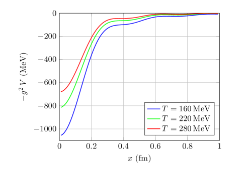
Refer to caption
Figure 2: The potential energy of a QQ¯𝑄¯𝑄Q\bar{Q} pair as a function of the Q𝑄Q-Q¯¯𝑄\bar{Q} distance x𝑥x for three different temperatures, and calculated with a cutoff Λ=4Λ4\Lambda=4 GeV. Much of the temperature dependence of the potential at small distance (x0.05fmsimilar-to𝑥0.05𝑓𝑚x\sim 0.05fm) can be attributed to that of the running coupling. The temperature dependence of the screening mass mDTsimilar-tosubscript𝑚𝐷𝑇m_{D}\sim T affects the potential in the intermediate range (x0.4fmsimilar-to𝑥0.4𝑓𝑚x\sim 0.4fm). The oscillations at intermediate and large distances are an artifact of the finite cutoff.

Consider first the real part V(𝐫)𝑉𝐫V({\mathbf{r}}). This is given by the screened Coulomb potential, which behaves as 1/r1𝑟1/r at short distance. This poses a well known problem in classical simulations. One way to see it is to notice that the classical distribution, that the Langevin equation eventually leads to, eβV(𝒓)similar-toabsentsuperscripte𝛽𝑉𝒓\sim{\rm e}^{-\beta V({\boldsymbol{r}})}, is singular at small r𝑟r for the attractive Coulomb potential. This would lead to an infinite probability for two particles to be close together. We may also observe that when two particles come to close to each other, their relative kinetic energy becomes big, and this violates the conditions of validity of the approximations used in Sect. 4 when deriving the classical equations. Note that this is a problem that arises only in the classical treatment of the Coulomb interaction through the Langevin equation; it would not occur if we were to solve the corresponding Schrödinger equation. A simple way out is to add a repulsive “quantum correction” in the form 2/2Mr2superscriptPlanck-constant-over-2-pi22𝑀superscript𝑟2\hbar^{2}/2Mr^{2}, as originally proposed by Kelbg [46]. Many refinements of this procedure have been studied (in the present context, see for instance [47] and references therein). In this exploratory work, we find it sufficient to turn off the force at short distance, as was done for instance in [35]. We do so here by introducing a finite cutoff in the integral Eq. (3.46) that yields the screened Coulomb potential. The resulting potential is displayed in Fig. 2. Note that when calculated with this prescription the value of the potential at the origin, V(0)𝑉0V(0), depends linearly on the cutoff, g2V(0)(2αs/π)Λsuperscript𝑔2𝑉02subscript𝛼𝑠𝜋Λg^{2}V(0)\approx(2\alpha_{s}/\pi)\Lambda. Therefore the cutoff ΛΛ\Lambda cannot be chosen too small otherwise the potential will not be deep enough to sustain bound states of the bottom quarks. Taking this into account, as well as further consideration to be presented shortly, we have settled for a value Λ=4Λ4\Lambda=4GeV, and this is the value with which the plots in Fig. 2 have been done. The temperature dependence that is seen in Fig. 2 arises mainly from the temperature dependence of the coupling constant, according to Eq. (5.82).

The presence of the cutoff makes the potential regular at short distance. One can then expand it around the origin and find the spring constant k𝑘k introduced in Sect. 4.3. We get

kmD3=16π2(Λ33mD3ΛmD+arctanΛmD).𝑘superscriptsubscript𝑚𝐷316superscript𝜋2superscriptΛ33superscriptsubscript𝑚𝐷3Λsubscript𝑚𝐷Λsubscript𝑚𝐷\displaystyle\frac{k}{m_{D}^{3}}=\frac{1}{6\pi^{2}}\left(\frac{\Lambda^{3}}{3m_{D}^{3}}-\frac{\Lambda}{m_{D}}+\arctan\frac{\Lambda}{m_{D}}\right). (5.83)

As mentioned in Sect. 4.3, the bound state will dissociate when the size, as measured by 𝒔2=3T/(g2k)delimited-⟨⟩superscript𝒔23𝑇superscript𝑔2𝑘\langle\bm{s}^{2}\rangle=3T/(g^{2}k) becomes of the order of the Debye radius, mD1superscriptsubscript𝑚𝐷1m_{D}^{-1}. Defining the corresponding temperature as TDsubscript𝑇𝐷T_{D}, we get (when ΛmDmuch-greater-thanΛsubscript𝑚𝐷\Lambda\gg m_{D})

TD4παs3mDkmD3.subscript𝑇𝐷4𝜋subscript𝛼𝑠3subscript𝑚𝐷𝑘superscriptsubscript𝑚𝐷3\displaystyle T_{D}\approx\frac{4\pi\alpha_{s}}{3}m_{D}\,\frac{k}{m_{D}^{3}}. (5.84)

For Λ=4Λ4\Lambda=4 GeV, mD=0.5subscript𝑚𝐷0.5m_{D}=0.5 Gev, this yields TD=320subscript𝑇𝐷320T_{D}=320 MeV, a reasonable order of magnitude. This provides another argument in favor of a not too small cutoff.
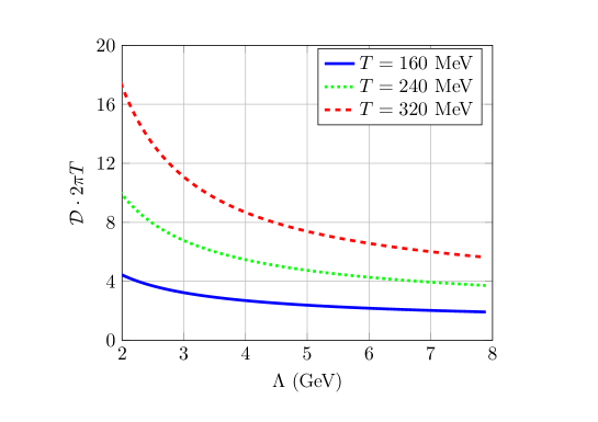
Refer to caption
Figure 3: The cutoff-dependence of the diffusion coefficient 𝒟=T/Mγ𝒟𝑇𝑀𝛾\mathcal{D}=T/M\gamma (see Eq. (4.78)), multiplied by 2πT2𝜋𝑇2\pi T, for different values of the temperature. Note that the differences between the three curves corresponding to different temperatures is largely due to the variation of the coupling constant, according to Eq. (5.82).

The second reason why we need a cutoff is that the second derivative of the imaginary part of the potential, that enters the definition of the friction, is divergent. This was already mentioned at the end of Sect. 3. The problem here is of a different nature as that of the real part. It reflects the fact that the hard thermal loop approximation used in the calculation of the imaginary part of the potential involves kinematical approximations that cease to be valid whenever large momentum exchanges are involved. Again the divergence can be controlled by a cutoff, which, here, would be naturally of the order of the temperature. In fact, we shall proceed as for the real part of the potential, and simply limit the momentum integral in Eq. (3.47) to values lower than ΛΛ\Lambda. Note that the values of ΛΛ\Lambda that are needed for V𝑉V and W𝑊W are a priori unrelated to each other. However, for simplicity and in order to avoid the proliferation of irrelevant parameters, we have performed calculations with a common value for ΛΛ\Lambda, independent of the temperature. It turns out that the drag coefficient and the diffusion constant depend only mildly on ΛΛ\Lambda around the value Λ=4Λ4\Lambda=4 GeV that we have adopted (see Fig. 3).

From the second derivative of W𝑊W we can calculate the drag coefficient, according to Eq. (4.77) and we get

γ=mD2e224πM(ln(1+Λ2mD2)Λ2Λ2+mD2),𝛾superscriptsubscript𝑚𝐷2superscript𝑒224𝜋𝑀1superscriptΛ2superscriptsubscript𝑚𝐷2superscriptΛ2superscriptΛ2superscriptsubscript𝑚𝐷2\displaystyle\gamma=\frac{m_{D}^{2}\,e^{2}}{24\,\pi\,M}\left(\ln\left(1+\frac{\Lambda^{2}}{m_{D}^{2}}\right)-\frac{\Lambda^{2}}{\Lambda^{2}+m_{D}^{2}}\right), (5.85)

To within a color factor CFsubscript𝐶𝐹C_{F} that we ignored, and with the specific choice Λ=TΛ𝑇\Lambda=T, this expression agrees with that obtained in Ref. [34] in the leading logarithm approximation. The diffusion constant 𝒟=T/(Mγ)𝒟𝑇𝑀𝛾\mathcal{D}={T}/({M\,\gamma}) is plotted in Fig. 3 as the dimensionless combination (2πT)𝒟2𝜋𝑇𝒟(2\pi T){\cal D}:

𝒟2πT=94αs2(ln(1+Λ2mD2)Λ2mD2Λ2mD2+1)1.𝒟2𝜋𝑇94superscriptsubscript𝛼𝑠2superscript1superscriptΛ2superscriptsubscript𝑚𝐷2superscriptΛ2superscriptsubscript𝑚𝐷2superscriptΛ2superscriptsubscript𝑚𝐷211\displaystyle\mathcal{D}\cdot 2\pi T=\frac{9}{4\alpha_{s}^{2}}\left(\ln\left(1+\frac{\Lambda^{2}}{m_{D}^{2}}\right)-\frac{\frac{\Lambda^{2}}{m_{D}^{2}}}{\frac{\Lambda^{2}}{m_{D}^{2}}+1}\right)^{-1}. (5.86)

One sees that in the region Λ4similar-to-or-equalsΛ4\Lambda\simeq 4 GeV, the diffusion constant depends indeed weakly on the value of ΛΛ\Lambda. Furthermore, for this value, 2πT𝒟2.72𝜋𝑇𝒟2.72\pi T{\cal D}\approx 2.7 for T=160𝑇160T=160 MeV, or γ0.2𝛾0.2\gamma\approx 0.2 fm-1. These values are of the order of magnitudes of those used in phenomenological studies [34] (see also [48] for more recent estimates).

Now that we have adjusted all the parameters, we can start exploring the main features of the dynamics of the heavy quarks in a plasma, as predicted by the generalized Langevin equation (4.72). The details of the numerical method that we use to solve this equation are given in Appendix C.

5.2 One heavy quark-antiquark pair

Our first set of results concerns the evolution of a heavy QQ¯𝑄¯𝑄Q\bar{Q} pair immersed in a uniform quark-gluon plasma in thermal equilibrium at temperature T𝑇T. The pair is prepared so that it corresponds initially to a bound state with a given size and binding energy. One first generates a sample of pairs, with the following procedure: The distance between the quark and the antiquark is chosen randomly between 00 and the Debye radius rD=mD1subscript𝑟𝐷superscriptsubscript𝑚𝐷1r_{D}=m_{D}^{-1}. The relative initial velocity of the quark and the antiquark is taken from a Maxwell distribution centered at the average value of typical quarkonia relative velocities (e.g. v020.3similar-tosuperscriptsubscript𝑣020.3v_{0}^{2}\sim 0.3 for charmonium [49]). Then we select from this sample the pairs that can be associated with specific bound states according to criteria that will be specified shortly. We then simulate the evolution of the pair using the Langevin equation (4.72) that was derived in Sect. 4.3.

As a first check of the Langevin dynamics, we consider a cc¯𝑐¯𝑐c\bar{c} pair at a temperature T=200𝑇200T=200 MeV. At this temperature, and for the parameters that we have chosen, all cc¯𝑐¯𝑐c\bar{c} bound states eventually dissociate in the plasma. This is what the plot on the left of Fig. 4 indeed shows. After an initial transient period of time, the two consituents of the pair follow independent Brownian motions, with the average distance squared growing linearly with time, in agreement with the analytical result, Eq. (4.78). Moreover, the right panel of Fig. 4 shows that the constituents indeed thermalize, the energy per quark reaching the value (3/2)T32𝑇(3/2)T, in agreement with the equipartition theorem.
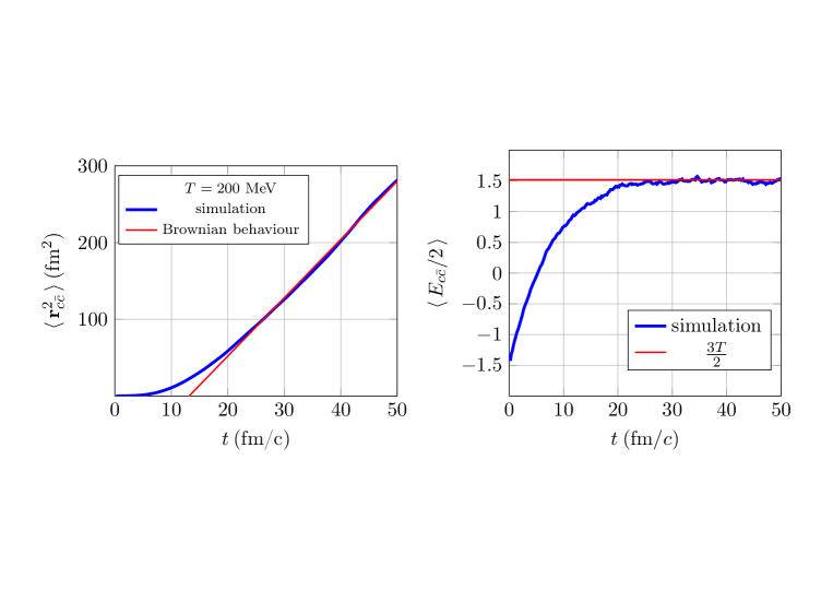
Refer to caption
Figure 4: On the left: Average c𝑐c-c¯¯𝑐\bar{c} distance squared as a function of time. This follows the predicted long-time Brownian behavior with the diffusion constant given by 𝒟2πT4𝒟2𝜋𝑇4\mathcal{D}\cdot 2\pi T\approx 4. On the right: Average energy (in 200200200 MeV units) per quark as a function of time compared with the energy at equilibrium (horizontal line). In both graphs we used T=200𝑇200T=200 MeV and Λ=4Λ4\Lambda=4 GeV. Statistical errors are to small to be plotted.

However, the very long time, where the heavy quarks eventually thermalize with the surrounding plasma, is not our main concern here. We want to understand the dynamics over shorter time scales, in particular because the plasma produced in a nucleus-nucleus collisions has a finite lifetime. To be specific, we shall take this lifetime to be τqgp10similar-tosubscript𝜏qgp10\tau_{\rm qgp}\sim 10\,fm/c, and accordingly our main focus will be to understand the dynamics of the heavy quarks over such a typical time scale. We shall also differentiate between different charmonium states, J/Ψ𝐽ΨJ/\Psi ( 11\,1S), χcsubscript𝜒𝑐\chi_{c} ( 11\,1P) and ΨsuperscriptΨ\Psi^{\prime} ( 22\,2S), but consider a single bottomonium state which we shall refer to as the ΥΥ\Upsilon. A word of explanation is needed here regarding what we mean by bound states. Within the classical simulation using the Langevin equation, this refers to the following procedure. At the beginning of the simulation we calculate the binding energy of a pair in its center of mass frame111111The binding energy is known at each time step of the simulation, since we follow both the velocities and the positions of the particles. and select the pairs according to the values of their initial radius r0subscript𝑟0r_{0}, and their binding energy ΔEΔ𝐸\Delta E\,. Depending on these values, we call a pair by the name of the closest bound state it would correspond to in a complete quantum treatment. The specific criteria that we use to attribute a charmonium state to a given pair are the following

  • 1.

    ΨsuperscriptΨ\Psi^{\prime}\qquad : 0<ΔE<1000Δ𝐸1000<\Delta E<100 MeV and r00.35subscript𝑟00.35r_{0}\geq 0.35 fm,

  • 2.

    χcsubscript𝜒𝑐\chi_{c}\qquad : 100ΔE300100Δ𝐸300100\leq\Delta E\leq 300 MeV and r00.25subscript𝑟00.25r_{0}\geq 0.25 fm,

  • 3.

    J/Ψ𝐽ΨJ/\Psi\quad\; : ΔE550Δ𝐸550\Delta E\geq 550 MeV and r00.10subscript𝑟00.10r_{0}\geq 0.10 fm,

  • 4.

    ΥΥ\Upsilon\qquad : ΔE700Δ𝐸700\Delta E\geq 700 MeV.

For the bottomonium, as already mentioned, we do not attempt to discriminate between the various bound states, and the requirement of a large binding energy automatically selects small sizes. In the case of charmonia, the constraint on the radius discriminates form instance a cc¯𝑐¯𝑐c\bar{c} pair with the binding energy of a ΨsuperscriptΨ\Psi^{\prime} but the radius of a χcsubscript𝜒𝑐\chi_{c}, and so forth. For the J/Ψ𝐽ΨJ/\Psi the minimum radius r0=0.1subscript𝑟00.1r_{0}=0.1 fm eliminates too high values of the binding energy. Such requirements do not apply to the ΥΥ\Upsilon\,, the binding energy being in this case limited by the depth of the potential (controlled by the cutoff ΛΛ\Lambda, as discussed in the previous subsection).

The time evolutions of the average size of pairs thus prepared are presented in Fig. 5 for different temperatures. The harmonic oscillator pattern expected from the analysis of Sect. 4.3 for pairs of small initial sizes is clearly visible. There are indeed cases where rqq¯delimited-⟨⟩subscript𝑟q¯q\langle\,r_{\rm q\bar{q}}\,\rangle remains almost constant for a certain time interval, reflecting the fact that the corresponding pair is highly correlated, or “bound”. The lower the temperature, the longer the correlation lasts. One also observes the expected “sequential melting” of ΨsuperscriptΨ\Psi^{\prime}\,, χcsubscript𝜒𝑐\chi_{c}\,, J/Ψ𝐽ΨJ/\Psi and ΥΥ\Upsilon as temperature grows. Of course the sequential dissociation of ΨsuperscriptΨ\Psi^{\prime}\,, χcsubscript𝜒𝑐\chi_{c}\,, J/Ψ𝐽ΨJ/\Psi just reflects the inequalities of their respective sizes, rΨ>rχc>rJ/Ψsubscript𝑟superscriptΨsubscript𝑟subscript𝜒𝑐subscript𝑟𝐽Ψr_{\Psi^{\prime}}>r_{\chi_{c}}>r_{J/\Psi}\,. One may try and attribute different “melting temperatures” to the dissociation of the various bound states. For example, we see from Fig. 5 that the initial plateau associated with the average ΨsuperscriptΨ\Psi^{\prime} radius is absent at T=220𝑇220T=220 MeV, indicating that ΨsuperscriptΨ\Psi^{\prime} immediately dissolves at this temperature, while the plateau is still visible at 190190190 MeV. One may then infer that the melting temperature of ΨsuperscriptΨ\Psi^{\prime} is T200𝑇200T\approx 200 MeV. Using the same argument of the size of the screening radius, we can extract a melting temperature of T310𝑇310T\approx 310 MeV for χcsubscript𝜒𝑐\chi_{c}\,. On the other hand, it is evident that the J/Ψ𝐽ΨJ/\Psi survives up to much higher temperatures than the other two charmonium states. However, for the J/Ψ𝐽ΨJ/\Psi we can not use the above strategy to estimate its melting temperature, because of the limitation of the numerical setup: when the temperature increases (T400greater-than-or-equivalent-to𝑇400\,T\gtrsim 400 MeV) it becomes impossible (with the present choice of parameters) to prepare an initial J/Ψ𝐽ΨJ/\Psi with ΔE550Δ𝐸550\Delta E\geq 550 MeV, the potential well is simply not deep enough (see Fig. 2). Later, we shall estimate the melting temperature of the J/Ψ𝐽ΨJ/\Psi by using a different procedure.

In the last panel of Fig. 5 we also compare the χcsubscript𝜒𝑐\chi_{c}\,, J/Ψ𝐽ΨJ/\Psi and ΥΥ\Upsilon behaviours at T=280𝑇280T=280 MeV. We see that the average bb¯𝑏¯𝑏b\bar{b} pair is far more strongly correlated than the cc¯𝑐¯𝑐c\bar{c} pair, and the ΥΥ\Upsilon radius remains small (rΥrD)\,\langle\,r_{\Upsilon}\,\rangle\leq r_{D}\,) for a relatively long time (we shall see in the next subsection that the melting temperature of the ΥΥ\Upsilon ( 11\,1S) state is T>600𝑇600T>600 MeV).

Refer to caption
Figure 5: (Color online.) Average quarkonia radius as a function of time. The pairs are prepared as “bound states” following the procedure explained in the text. The shaded part indicates the region in which the charmonia radii are smaller than the Debye radius rDsubscript𝑟𝐷r_{D}. Statistical errors are too small to be plotted. In each plot, the upper curve represent the less bound system, the lower curve the most bound one.

The curves representing the χcsubscript𝜒𝑐\chi_{c} exhibit an interesting phenomenon. One sees that in all cases, the corresponding radius tends to decrease initially, bringing the χcsubscript𝜒𝑐\chi_{c} closer to a more stable bound state (J/Ψ𝐽ΨJ/\Psi). This is a clear indication that, at these temperatures, the binding forces are not yet entirely screened. While on average, the relative kinetic energy prevents the χcsubscript𝜒𝑐\chi_{c} to really decay into a J/Ψ𝐽ΨJ/\Psi, as the curves in Fig. 5 indicate, a substantial fraction of the pairs prepared as χcsubscript𝜒𝑐\chi_{c} does decay into J/ψ𝐽𝜓J/\psi’s, as shown in Fig. 6. It is possible to estimate the percentages of χcsubscript𝜒𝑐\chi_{c} and ΨsuperscriptΨ\Psi^{\prime} states that decay into J/Ψ𝐽ΨJ/\Psi\,, a process known as feed-down. In Table 1 the feed-down percentages of χcsubscript𝜒𝑐\chi_{c} and ΨsuperscriptΨ\Psi^{\prime} are listed for some values of the temperature. We found that, for each temperature, there are more χcsubscript𝜒𝑐\chi_{c} than ΨsuperscriptΨ\Psi^{\prime} states that decay into J/Ψ𝐽ΨJ/\Psi\,, and the feed-down mechanism decreases when the temperature grows: the more fragile states prefer to dissociate rather than form a more strongly bound system. Amusingly, the feed-down fractions obtained here at T=190𝑇190T=190 MeV are similar to the experimental values quoted in [50], although of course the physical context is rather different.

T𝑇T (MeV) 160 190 220 280
χcsubscript𝜒𝑐\chi_{c} (40-43)% (28-30)% (16-17)% (1-2)%
ΨsuperscriptΨ\Psi^{\prime} (12-14)% (7-8)% 0% /
Table 1: Fractions of χcsubscript𝜒𝑐\chi_{c} and ΨsuperscriptΨ\Psi^{\prime} eventually becoming J/Ψ𝐽ΨJ/\Psi’s.

In Fig. 6 we compare the different behaviors of the χcsubscript𝜒𝑐\chi_{c} and ΨsuperscriptΨ\Psi^{\prime} average radii, separating those which decay from those which do not. Looking on the left of Fig. 6 we notice that even the non-decaying χcsubscript𝜒𝑐\chi_{c} states initially reduce (on average) their radius (also at T=280𝑇280T=280 MeV, as seen in the last panel of Fig. 5). This why their average lifetime (see Table 2) remains almost the same below the melting temperature (310absent310\approx 310 MeV), whereas the average lifetime of a non-decaying ΨsuperscriptΨ\Psi^{\prime} diminishes as the temperature goes up.

The lifetimes of Table 2 are calculated by averaging the time intervals needed for the radii of χcsubscript𝜒𝑐\chi_{c}\,, ΨsuperscriptΨ\Psi^{\prime} (both not-decaying) and J/Ψ𝐽ΨJ/\Psi to become larger than the Debye screening length. One notices that the J/Ψ𝐽ΨJ/\Psi lifetime at T=280𝑇280T=280 MeV is still quite appreciable.

Refer to caption
Figure 6: (Color online.) On the left: Comparison between rcc¯delimited-⟨⟩subscript𝑟𝑐¯𝑐\langle\,r_{c\bar{c}}\,\rangle of χcsubscript𝜒𝑐\chi_{c} states that become J/Ψ𝐽ΨJ/\Psi (41%absentpercent41\approx 41\% – lower curve) and those that do not decay (59%absentpercent59\approx 59\% – upper curve). On the right: Same comparison for ΨsuperscriptΨ\Psi^{\prime}\,. The pairs are prepared as bound states as indicated in the text. For similar initial conditions, they evolve statistically to different final states.
T𝑇T (MeV) 160 190 220 280
J/Ψ𝐽ΨJ/\Psi 10greater-than-or-equivalent-toabsent10\gtrsim 10 10greater-than-or-equivalent-toabsent10\gtrsim 10 4.9±plus-or-minus\pm 0.2 2.8±plus-or-minus\pm 0.2
χcsubscript𝜒𝑐\chi_{c} 1.6±plus-or-minus\pm 0.1 1.6±plus-or-minus\pm 0.1 1.5±plus-or-minus\pm 0.1 1.6±plus-or-minus\pm 0.1
ΨsuperscriptΨ\Psi^{\prime} 0.7±plus-or-minus\pm 0.1 0.5±plus-or-minus\pm 0.1 0.1±plus-or-minus\pm 0.1 0
Table 2: Average charmonium lifetimes (in fm/c) in the quark-gluon plasma. Only the χcsubscript𝜒𝑐\chi_{c} and ΨsuperscriptΨ\Psi^{\prime} that do not decay into J/Ψ𝐽ΨJ/\Psi are taken into account in the lifetime estimates.

5.3 Many heavy quark-antiquark pairs

In the previous subsection, we saw how a single heavy quark antiquark pair can evolve from an apparent bound state to a system of two independent quarks that eventually thermalize with the plasma on long time scales. We could also observe, with a proper selection of the initial conditions the expected phenomenon of sequential dissociations. Finally, we provided some criterion to get a crude estimate of the lifetime of the bound state in the plasma. We would like now to examine how these features are modified when several pairs are present in the plasma.
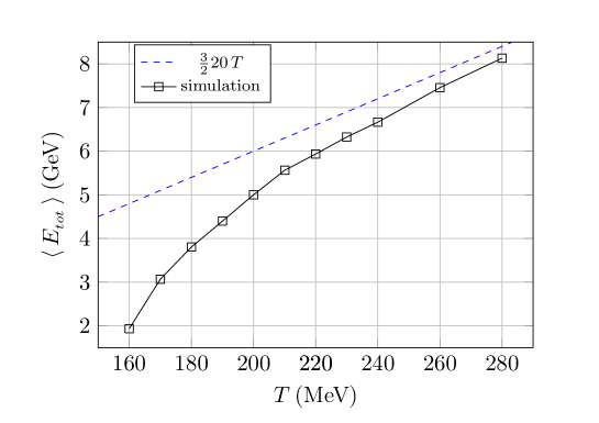
Refer to caption
Figure 7: Average total energy of a system of 101010 cc¯𝑐¯𝑐c\bar{c} pairs in thermal equilibrium as a function of temperature. Before measuring the energies, we ran the simulations for a time interval of 100100100 fm in order to let the system thermalize. Simulations were performed in a periodic cubic box of side 444 fm and statistical errors are again too small to be plotted.

The simulations that we shall present were performed for N=2,10𝑁210N=2,10 and 505050 quark-antiquark pairs, in a cubic box of side 444 fm, with periodic boundary conditions.

When there are enough pairs in the system, one expects them to evolve towards an ideal gas of the constituents, if the temperature is high enough. The average energy for a system of N=10𝑁10N=10 pairs is plotted in Fig. 7, and compared to that of an ideal monoatomic gas of 2N2𝑁2N particles,

Egas=32(2N)KBT.subscript𝐸gas322𝑁subscript𝐾𝐵𝑇\displaystyle E_{\rm gas}=\frac{3}{2}(2N)\,K_{B}T. (5.87)

The expected trend is clearly visible, and at the largest temperatures considered, T280greater-than-or-equivalent-to𝑇280T\gtrsim 280 MeV, the ideal gas limit is almost reached. At such high temperatures, most of the pairs dissociate if one waits long enough. On the other hand, at lower temperatures, pairs may survive and this results in the average energy of the system being lower than that of the ideal gas at the same temperature. We note that the process of dissociation, considered from this thermodynamical point of view, is a gradual process: even at high temperature there remains some finite probability to find a bound pair. Given the length of the simulation (over 100100100 fm/c), and that, in this range of temperatures, a single pair would eventually dissociate, the equilibrium state that we are observing results from the balance of the two competing effects of dissociation and recombination, as we shall discuss in more details shortly.
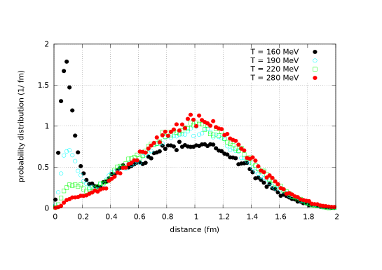
Refer to caption
Figure 8: The figure shows the distribution of distances to the nearest antiquark from a given quark. This probability is computed in the following way: once thermal equilibrium is reached, one computes from each quark the distance to the nearest antiquark, draw an histogram, and normalize in order to get the distribution. Simulations were performed for a system of 10 cc¯𝑐¯𝑐c\bar{c} pairs in a cubic box of side 444 fm, with periodic boundary conditions.

The presence of bound pairs in the system can also be inferred form the analysis of another quantity that is directly sensitive to the correlations between two particles, namely the probability distribution Pqq¯subscript𝑃𝑞¯𝑞P_{q\bar{q}} of the distance from a given quark to the nearest antiquark. In an ideal gas, this distribution is given by

Pqq¯ideal(r)=3a(ra)2(1(ra)31N)N1N13a(ra)2e(r/a)13,subscriptsuperscript𝑃ideal𝑞¯𝑞𝑟3𝑎superscript𝑟𝑎2superscript1superscript𝑟𝑎31𝑁𝑁1superscriptsimilar-to-or-equalsmuch-greater-than𝑁13𝑎superscript𝑟𝑎2superscript𝑒superscript𝑟𝑎13P^{\rm ideal}_{q\bar{q}}(r)=\frac{3}{a}\!\left(\frac{r}{a}\right)^{\!2}\!\left(1-\left(\frac{r}{a}\right)^{3}\!\frac{1}{N}\right)^{\!\!N-1}\stackrel{{\scriptstyle N\gg 1}}{{\simeq}}\frac{3}{a}\left(\frac{r}{a}\right)^{2}e^{-(r/a)^{\frac{1}{3}}}\>,

where a=(34πρ)1/3𝑎superscript34𝜋𝜌13a=\left(\frac{3}{4\pi\rho}\right)^{1/3} is the mean distance between the antiquarks and ρ=NV𝜌𝑁𝑉\rho=\frac{N}{V}\, the density of antiquarks. The peak of the ideal gas distribution for N=10𝑁10N=10 quark-antiquark pairs in a cubic box of side 444 fm, is at rpeak=(2029)1/3a1.15subscript𝑟peaksuperscript202913𝑎1.15r_{\rm peak}=(\frac{20}{29})^{1/3}a\approx 1.15 fm. This peak is clearly visible in the distribution Pqq¯subscript𝑃𝑞¯𝑞P_{q\bar{q}} of the interacting system which is plotted in Fig. 8. But this figure reveals also another feature: at low temperature, there is also a sharper peak reflecting the presence of highly correlated states in the system. These, we associate with the bound states. In line with the previous plot, Fig. 7, this peak disappears when T280greater-than-or-equivalent-to𝑇280T\gtrsim 280 MeV. From Fig. 8 we can also infer that a correlated cc¯𝑐¯𝑐c\bar{c} pair has a maximum radius of approximately 0.30.30.3 fm, which is indeed similar to the values of the Debye screening length in this range of temperature.

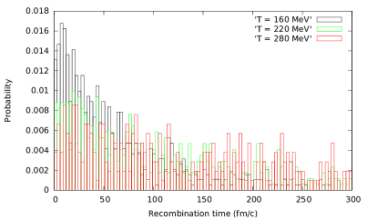
Refer to caption
Refer to caption
Figure 9: On the left: Average recombination time as a function of temperature. On the right: Probability of recombination times for three values of temperatures. The quark-antiquark distance has been chosen to be less or equal to 0.30.30.3 fm for the quark-antiquark configuration to be considered a pair (see text). Both simulations were performed with a system of 10 cc¯𝑐¯𝑐c\bar{c} pairs in a cubic box of side 444 fm, with periodic boundary conditions.

We turn now to a more detailed study of the process of recombination. We start with the evaluation of the recombination times for the pairs as a function of the temperature, that is the average time needed for a quark (antiquark) to form a pair, once the quark (antiquark) moves away from its previous antiquark (quark) partner. In doing this calculation we carefully avoid counting the contributions of “non-interacting” events, that is the occurrences where a quark passes by an antiquark without forming an actual pair. In order to eliminate such events, we performed simulations for a non-interacting system with a constant (space-independent) drag constant (see Eq. (4.77)) and we calculated the corresponding normalized distribution Pfree(t)subscript𝑃free𝑡P_{\rm free}(t) of the time intervals t𝑡t in which a charm and an anticharm stay close together within a sphere of radius 0.30.30.3 fm. Then, for each temperature, we define a minimum lifetime τ𝜏\tau by the condition

τdtPfree(t)<1%.superscriptsubscript𝜏differential-d𝑡subscript𝑃free𝑡percent1\displaystyle\int_{\tau}^{\infty}{\rm d}t\,P_{\rm free}(t)<1\%\>. (5.88)

By selecting pairs that stay together for a time greater than τ𝜏\tau, only pairs formed because of the interactions (and not those resulting from random encounters) contribute to the recombination times. Note that the procedure does not allow for a detailed analysis in terms of various bound states, as we were able to do for the dissociation: the small lifetimes typical of χcsubscript𝜒𝑐\chi_{c} and ΨsuperscriptΨ\Psi^{\prime} are automatically discarded by the procedure, so that we implicitly consider only J/Ψ𝐽ΨJ/\Psi regeneration.

As one can see on the left of Fig. 9, the outcome for a system of 101010 cc¯𝑐¯𝑐c\bar{c} pairs is that the recombination time increases almost linearly with the temperature, starting from a value of trec=(62.9±2.5)subscript𝑡recplus-or-minus62.92.5t_{\rm rec}=(62.9\pm 2.5) fm at T=160𝑇160T=160 MeV and reaching a value of trec=(185.5±6.8)subscript𝑡recplus-or-minus185.56.8t_{\rm rec}=(185.5\pm 6.8) fm at T=280𝑇280T=280 MeV. As one increases the temperature one increases the rate of encounters, but also the relative kinetic energies of the pairs, preventing binding. Another important observation is that the recombination times are very long, so long that one may wonder whether the mechanism of recombination could be of any phenomenological relevance. However, as the graph on the right panel of Fig. 9 shows, the distribution of the recombination times is very broad. Thus, even if the standard errors of the graph on the left panel of Fig. 9 are small (because of the large statistics), the standard deviations are of the same order as the average values: over the lifetime of the quark-gluon plasma (10similar-toabsent10\sim 10 fm/c) there is effectively no characteristic time scale for recombination.

One can nevertheless push the discussion a bit further and quantify the process in a simple way. Note first that the recombination time is expected to go up when the number of particles decreases. This is indeed what we obtain from our simulations. We find that the average recombination time is, to a good approximation, inversely proportional to the number of pairs present in the system: trecNλR1subscript𝑡rec𝑁superscriptsubscript𝜆𝑅1t_{\rm rec}N\approx\lambda_{R}^{-1}\,, with λRsubscript𝜆𝑅\lambda_{R} a (temperature-dependent) recombination rate. This effect is also (qualitatively) visible in Fig. 10 that displays the fraction of surviving J/Ψ𝐽ΨJ/\Psi (and ΥΥ\Upsilon) particles as a function of time, for different number of pairs in the system: one notices that recombination events are more frequent in a system with a greater number of cc¯𝑐¯𝑐c\bar{c} pairs. One may also observe that the effect of recombination becomes relatively more important as the temperature grows. This is visible for instance from the development of a plateau suggestive of equilibrium that is most clearly seen at the highest temperature (T=220𝑇220T=220 MeV). Finally, the last panel of Fig. 10 compares the behaviors of cc¯𝑐¯𝑐c\bar{c} and bb¯𝑏¯𝑏b\bar{b} at a given temperature over a long time scale. One sees that there is a lapse of time before the bb¯𝑏¯𝑏b\bar{b} bound state starts to “feel” the action of the thermal medium. This time delay t0subscript𝑡0t_{0} is about t04subscript𝑡04t_{0}\approx 4 fm/c. A similar effect also occurs for charmonium, but for a smaller t01less-than-or-similar-tosubscript𝑡01t_{0}\lesssim 1 fm/c. This dependence on the mass is a clear indication of the important role of the collisions in the dissociation process.

At the same time, the effect of the binding forces is certainly also present. This we see indirectly by studying the cutoff dependence of the results. To that aim, we have repeated simulations for various values of the cutoff. As we have seen earlier, the dominant effect of a change in the cutoff is to change the depth of the potential. A larger cutoff leads to a deeper potential, and a longer lifetime, and this effect persists up to values of the order Λ6Λ6\Lambda\approx 6 GeV, above which it attenuates considerably. In turns, this alters the recombination rates since the pairs with too short lifetimes are eliminated by the procedure with which we identify bound pairs.

One may understand quantitatively the behaviors identified in Fig. 10 from a simple rate equation. Let us denote by λD(T)subscript𝜆𝐷𝑇\lambda_{D}(T) the dissociation rate and by λR(T)subscript𝜆𝑅𝑇\lambda_{R}(T) the recombination rate. Both are functions of the temperature.
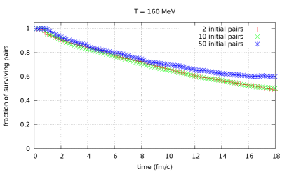
Refer to caption
Refer to caption
Refer to caption
Refer to caption
Figure 10: Fraction of surviving pairs as a function of time for three different temperatures. The N𝑁N pairs (N=2,10,50𝑁21050N=2,10,50) are prepared at t=0𝑡0t=0 as bound states as indicate earlier in the text. The short time behavior is dominated by dissociation. The process starts however only after some small delay t01less-than-or-similar-tosubscript𝑡01t_{0}\lesssim 1 fm/c. This delay is much longer the the bottomonium, as revealed by the comparison displayed in the bottom-right panel: fraction of surviving J/Ψ𝐽ΨJ/\Psi and ΥΥ\Upsilon, for a system of N=10𝑁10N=10 c𝑐c-c¯¯𝑐\bar{c} or b𝑏b-b¯¯𝑏\bar{b} pairs. Simulations were performed in a periodic cubic box of side 444 fm.

The rate equation describing the time evolution of the number of surviving QQ¯𝑄¯𝑄Q\bar{Q} pairs N(t)𝑁𝑡N(t) is (see also [10])

dN(t)dt=λDN(t)+λRNq(t)Nq¯(t),d𝑁𝑡d𝑡subscript𝜆𝐷𝑁𝑡subscript𝜆𝑅subscript𝑁𝑞𝑡subscript𝑁¯𝑞𝑡\displaystyle\frac{\mathop{}\!\mathrm{d}N(t)}{\mathop{}\!\mathrm{d}t}=-\lambda_{D}N(t)+\lambda_{R}N_{q}(t)N_{\bar{q}}(t)\>, (5.89)

where Nq=Nq¯subscript𝑁𝑞subscript𝑁¯𝑞N_{q}=N_{\bar{q}}\, is the number of free heavy quarks (or antiquarks) in the plasma. Equation (5.89) together with the initial condition N(t=t0)=N0𝑁𝑡subscript𝑡0subscript𝑁0N(t=t_{0})=N_{0}\,, Nq¯(t0)=Nq(t0)=0subscript𝑁¯𝑞subscript𝑡0subscript𝑁𝑞subscript𝑡00N_{\bar{q}}(t_{0})=N_{q}(t_{0})=0 can be analytically solved for the fraction of surviving pairs:

N(t)N0=1λDΩtanh(Ω2(tt0))1+λDΩtanh(Ω2(tt0)),tt0,formulae-sequence𝑁𝑡subscript𝑁01subscript𝜆𝐷ΩΩ2𝑡subscript𝑡01subscript𝜆𝐷ΩΩ2𝑡subscript𝑡0𝑡subscript𝑡0\displaystyle\frac{N(t)}{N_{0}}=\frac{1-\frac{\lambda_{D}}{\Omega}\tanh\left(\frac{\Omega}{2}(t-t_{0})\right)}{1+\frac{\lambda_{D}}{\Omega}\tanh\left(\frac{\Omega}{2}(t-t_{0})\right)}\>,\qquad t\geq t_{0}\>, (5.90)

where ΩλD(λD+4λRN0)Ωsubscript𝜆𝐷subscript𝜆𝐷4subscript𝜆𝑅subscript𝑁0\Omega\equiv\sqrt{\lambda_{D}(\lambda_{D}+4\lambda_{R}N_{0})} and we used Nq(t)=Nq¯(t)=N0N(t)subscript𝑁𝑞𝑡subscript𝑁¯𝑞𝑡subscript𝑁0𝑁𝑡N_{q}(t)=N_{\bar{q}}(t)=N_{0}-N(t). The time t0subscript𝑡0t_{0} is the time at which dissociation starts, as defined earlier, and this time is chosen as the initial time when solving the rate equation (5.89).

T𝑇T (MeV) λD1(fm/c)superscriptsubscript𝜆𝐷1fm/c\lambda_{D}^{-1}\,(\mbox{fm/c}) λR1(fm/c)superscriptsubscript𝜆𝑅1fm/c\lambda_{R}^{-1}\,(\mbox{fm/c})
160 23 625
190 9.2 1000
220 4.6 1350
Table 3: The inverse of the dissociation rate λD1superscriptsubscript𝜆𝐷1\lambda_{D}^{-1} and the recombination rate λR1superscriptsubscript𝜆𝑅1\lambda_{R}^{-1}, for various temperatures.
Refer to caption
Refer to caption
Figure 11: Left panel: fit of the solution (5.90) of the rate equation for a system of 101010 initial J/Ψ𝐽ΨJ/\Psi at three different temperatures. We notice that eq.(5.90) fits the curves very well with the recombination rates λRsubscript𝜆𝑅\lambda_{R} equal to the ones derived in Fig. 9. Right panel: high temperature behaviour of charmonium and bottomonium.

From the results of the simulations, and using Eq. (5.90), we can extract values for the dissociation and regeneration rates. The results are reported in Table 3 for a few temperatures. The quality of the fit can be seen on Fig. 11. The values of the dissociation rate thus determined can be used to infer the lifetimes of the bound states. The values of the J/Ψ𝐽ΨJ/\Psi lifetimes obtained from the present fit agree with those previously obtained by analyzing the time evolution of the J/Ψ𝐽ΨJ/\Psi radius (see Table 2). The analysis of the values of the dissociation rate just obtained suggests that at a temperature T=600𝑇600T=600 MeV, the lifetime of the J/ψ𝐽𝜓J/\psi is still non vanishing, and is about .5 fm/c. At the same temperature, the lifetime of the ΥΥ\Upsilon is about 1.51.51.5 fm/c. The fit of bottomonium data gives essentially zero recombination rates already at T=160𝑇160T=160 MeV (λR(1±1)105similar-tosubscript𝜆𝑅plus-or-minus11superscript105\,\lambda_{R}\sim(1\pm 1)\cdot 10^{-5} fm/c) and much smaller values of the dissociation rate as compared to the charmonium case. These numbers reflect of course the greater stability of the ΥΥ\Upsilon as compared to the J/Ψ𝐽ΨJ/\Psi.

6 Conclusions

We have presented an approach that treats in a unique framework most of the important aspects of the evolution of a collection of heavy quark-antiquark pairs propagating through a quark gluon plasma. The approach starts from first principles, and leads, through well defined approximations, to a complete dynamical description with a unified perspective on many different physical effects, usually treated with different models. Of course, several approximations are needed to arrive at tractable calculations. However these approximations can be improved, and their presence should not obscure the overall consistency of the general scheme. We find it particularly important, for instance, in view of their relevance for the interpretation of the data, to have the processes of dissociation and recombination treated on the same footing.

The main question that is addressed in this paper is of a general nature, it concerns the fate of a collection of heavy quark pairs in a hot and dense environment, with the possibility for these heavy particles to form bound states. This does not involve QCD dynamics in an essential way, and this is the main reason why we have restricted ourselves in this paper to Abelian plasmas where the same question can be addressed in a much simpler setting. Specific features of QCD can be implemented within the present scheme, with perhaps some approximations becoming less accurate. In particular, one of the main approximations can be understood as a weak coupling approximation, which consists in neglecting the non linear coupling of the gauge (Coulomb) field with which the particles interact. The field fluctuations are then Gaussian, which allows for a simple calculation of the influence functional in terms of a 2-point function that characterizes entirely the effect of the plasma on the heavy particles. In QCD, the non linear couplings are not as strongly suppressed as in QED, and the approximation may be less accurate.

Further approximations lead to a classical treatment of the dynamics in terms of a Langevin equation, in which the noise term accounts for the effect of the collisions between the heavy particles and the plasma constituents. This noise terms depends on the positions of the heavy quarks at each time steps. This dependence is an important aspect of the dynamics.

The simulations presented in this paper are the first in a program that can be improved in many ways. Some of the approximations that have been made can easily be relaxed, such as for instance the Abelian approximation, as we have discussed already. The classical treatment of the dynamics through a Langevin equation could be improved, e.g. including the leading order quantum corrections to the Langevin equation, as shown in [57]. The basic ingredients such as the transport coefficients, can be calculated with greater accuracy. Finally, once some of these improvements are implemented, more realistic phenomenological applications can be envisaged. We hope to be able to report on some of these developments soon.

Acknowledgements

This research is supported by the European Research Council under the Advanced Investigator Grant ERC-AD-267258. JPB acknowledges early discussions on some aspects of this project with F. Dominguez and B. Wu, as well as with Y. Akamatsu. GG acknowledges support by Istituto Nazionale di Fisica Nucleare through the “Supercalcolo” agreement with Fondazione Bruno Kessler. Computer simulations were performed on the KORE computing cluster at FBK.

Appendix A Taylor expansion of the Influence Functional

In this Appendix, we perform the Taylor expansion of Φ[𝑸]=ΦQQ[𝑸]+ΦQ¯Q¯[𝑸]+ΦQQ¯[𝑸]Φdelimited-[]𝑸subscriptΦ𝑄𝑄delimited-[]𝑸subscriptΦ¯𝑄¯𝑄delimited-[]𝑸subscriptΦ𝑄¯𝑄delimited-[]𝑸\Phi[{\boldsymbol{Q}}]=\Phi_{{}_{QQ}}[{\boldsymbol{Q}}]+\Phi_{{}_{\bar{Q}\bar{Q}}}[{\boldsymbol{Q}}]+\Phi_{{}_{Q\bar{Q}}}[{\boldsymbol{Q}}] obtained from Eqs. (4.57) and (4.1) of section 4 after performing the change of coordinates of Eq. (4.59). We first analyze the contribution ΦQQ[𝑸]subscriptΦ𝑄𝑄delimited-[]𝑸\Phi_{{}_{QQ}}[{\boldsymbol{Q}}] involving only the heavy quarks. We have

ΦQQ[𝐑,𝐘]=g22i,j=1Ntitfdt{V(𝐫j𝐫i𝒚j2+𝒚i2)V(𝐫j𝐫i+𝒚j2𝒚i2)\displaystyle\Phi_{{}_{QQ}}[{\mathbf{R}},{\mathbf{Y}}]=\frac{g^{2}}{2}\sum_{i,j=1}^{N}\int_{t_{i}}^{t_{f}}\mathop{}\!\mathrm{d}{t}\left\{V\left({\mathbf{r}}_{j}-{\mathbf{r}}_{i}-\frac{{\boldsymbol{y}}_{j}}{2}+\frac{{\boldsymbol{y}}_{i}}{2}\right)-V\left({\mathbf{r}}_{j}-{\mathbf{r}}_{i}+\frac{{\boldsymbol{y}}_{j}}{2}-\frac{{\boldsymbol{y}}_{i}}{2}\right)\right.
iW(𝐫j𝐫i𝒚j2+𝒚i2)iW(𝐫j𝐫i+𝒚j2𝒚i2)+2iW(𝐫j𝐫i+𝒚j2+𝒚i2)i𝑊subscript𝐫𝑗subscript𝐫𝑖subscript𝒚𝑗2subscript𝒚𝑖2i𝑊subscript𝐫𝑗subscript𝐫𝑖subscript𝒚𝑗2subscript𝒚𝑖22i𝑊subscript𝐫𝑗subscript𝐫𝑖subscript𝒚𝑗2subscript𝒚𝑖2\displaystyle\left.-\mathrm{i}W\left({\mathbf{r}}_{j}-{\mathbf{r}}_{i}-\frac{{\boldsymbol{y}}_{j}}{2}+\frac{{\boldsymbol{y}}_{i}}{2}\right)-\mathrm{i}W\left({\mathbf{r}}_{j}-{\mathbf{r}}_{i}+\frac{{\boldsymbol{y}}_{j}}{2}-\frac{{\boldsymbol{y}}_{i}}{2}\right)+2\,\mathrm{i}W\left({\mathbf{r}}_{j}-{\mathbf{r}}_{i}+\frac{{\boldsymbol{y}}_{j}}{2}+\frac{{\boldsymbol{y}}_{i}}{2}\right)\right.
β2(𝐫˙j+𝐫˙i+𝒚˙j2𝒚˙i2)(12𝐫j+𝒚j)W(𝐫j𝐫i+12𝒚j+12𝒚i)},\displaystyle\left.-\frac{\beta}{2}\left(\dot{{\mathbf{r}}}_{j}+\dot{{\mathbf{r}}}_{i}+\frac{\dot{{\boldsymbol{y}}}_{j}}{2}-\frac{\dot{{\boldsymbol{y}}}_{i}}{2}\right)\cdot\left(\frac{1}{2}\frac{\partial}{\partial{\mathbf{r}}_{j}}+\frac{\partial}{\partial{\boldsymbol{y}}_{j}}\right)W\left({\mathbf{r}}_{j}-{\mathbf{r}}_{i}+\frac{1}{2}{\boldsymbol{y}}_{j}+\frac{1}{2}{\boldsymbol{y}}_{i}\right)\right\},

where the time dependence is hidden in the coordinates 𝐑𝐑{\mathbf{R}} and 𝐘𝐘{\mathbf{Y}}. The dot symbol in this expression, as well as in the rest of this section, denotes a scalar product and involves the three cartesian components of the vectors. We want to expand the expression (A) to second order in 𝒚𝒚{\boldsymbol{y}}. To do so, we use the well-known Taylor expansion of a scalar function f𝑓f of a n𝑛n-dimensional vector 𝒙𝒙{\boldsymbol{x}},

f(𝒙)=f(𝐚)+(𝒙𝐚)f(𝐚)+12(𝒙𝐚)f(𝐚)(𝒙𝐚)+𝑓𝒙𝑓𝐚𝒙𝐚bold-∇𝑓𝐚12𝒙𝐚superscript𝑓𝐚𝒙𝐚\displaystyle f({\boldsymbol{x}})=f({\mathbf{a}})+({\boldsymbol{x}}-{\mathbf{a}})\cdot{\boldsymbol{\nabla}}f({\mathbf{a}})+\frac{1}{2}\leavevmode\nobreak\ ({\boldsymbol{x}}-{\mathbf{a}})\cdot\mathcal{H}^{f}({\mathbf{a}})\cdot({\boldsymbol{x}}-{\mathbf{a}})+\dots

where 𝒙=(x1,,xn)𝒙subscript𝑥1subscript𝑥𝑛{\boldsymbol{x}}=(x_{1},\dots,x_{n}), and the gradient and Hessian matrix are given, as usual, by

αf(𝐚):=f(𝒙)xα|𝒙=𝐚,αβf(𝐚):=2f(𝒙)xαxβ|𝒙=𝐚,α,β=1,,n.formulae-sequenceassignsubscript𝛼𝑓𝐚evaluated-at𝑓𝒙subscript𝑥𝛼𝒙𝐚formulae-sequenceassignsuperscriptsubscript𝛼𝛽𝑓𝐚evaluated-atsuperscript2𝑓𝒙subscript𝑥𝛼subscript𝑥𝛽𝒙𝐚𝛼𝛽1𝑛\displaystyle\nabla_{\alpha}f({\mathbf{a}}):=\left.\frac{\partial f({\boldsymbol{x}})}{\partial x_{\alpha}}\right|_{{\boldsymbol{x}}={\mathbf{a}}},\qquad\mathcal{H}_{\alpha\beta}^{f}({\mathbf{a}}):=\left.\frac{\partial^{2}f({\boldsymbol{x}})}{\partial x_{\alpha}\partial x_{\beta}}\right|_{{\boldsymbol{x}}={\mathbf{a}}}\;,\qquad\alpha,\beta=1,\cdots,n. (A.92)

By applying this formula to the first line of Eq. (A) we get (with 𝐫ji𝐫j𝐫isubscript𝐫𝑗𝑖subscript𝐫𝑗subscript𝐫𝑖{\mathbf{r}}_{ji}\equiv{\mathbf{r}}_{j}-{\mathbf{r}}_{i}, 𝒚ji𝒚j𝒚isubscript𝒚𝑗𝑖subscript𝒚𝑗subscript𝒚𝑖{\boldsymbol{y}}_{ji}\equiv{\boldsymbol{y}}_{j}-{\boldsymbol{y}}_{i})

V(𝐫ji12𝒚ji)V(𝐫ji+12𝒚ji)=𝒚jiV(𝐫ji).𝑉subscript𝐫𝑗𝑖12subscript𝒚𝑗𝑖𝑉subscript𝐫𝑗𝑖12subscript𝒚𝑗𝑖subscript𝒚𝑗𝑖bold-∇𝑉subscript𝐫𝑗𝑖\displaystyle V({\mathbf{r}}_{ji}-\frac{1}{2}{\boldsymbol{y}}_{ji})-V({\mathbf{r}}_{ji}+\frac{1}{2}{\boldsymbol{y}}_{ji})=-{\boldsymbol{y}}_{ji}\cdot{\boldsymbol{\nabla}}V({\mathbf{r}}_{ji}). (A.93)

Similarly121212The Hessian matrix of W𝑊W is the only such matrix in the present discussion, so we denote it simply by \mathcal{H}, without any explicit reference to W𝑊W in the notation. That is, in the notation of Eq. (A.92), Wsuperscript𝑊\mathcal{H}\equiv\mathcal{H}^{{}_{W}}.,

W(𝐫ji12𝒚ji)W(𝐫ji+12𝒚ji)=2W(𝐫ji)14𝒚ji(𝐫ji)𝒚ji,𝑊subscript𝐫𝑗𝑖12subscript𝒚𝑗𝑖𝑊subscript𝐫𝑗𝑖12subscript𝒚𝑗𝑖2𝑊subscript𝐫𝑗𝑖14subscript𝒚𝑗𝑖subscript𝐫𝑗𝑖subscript𝒚𝑗𝑖\displaystyle-W({\mathbf{r}}_{ji}-\frac{1}{2}{\boldsymbol{y}}_{ji})-W({\mathbf{r}}_{ji}+\frac{1}{2}{\boldsymbol{y}}_{ji})=-2W({\mathbf{r}}_{ji})-\frac{1}{4}\,{\boldsymbol{y}}_{ji}\cdot\mathcal{H}({\mathbf{r}}_{ji})\cdot{\boldsymbol{y}}_{ji}, (A.94)

and (with 𝒚~ji𝒚j+𝒚isubscript~𝒚𝑗𝑖subscript𝒚𝑗subscript𝒚𝑖\tilde{\boldsymbol{y}}_{ji}\equiv{\boldsymbol{y}}_{j}+{\boldsymbol{y}}_{i})

W(𝐫ji+𝒚~ji2)=W(𝐫ji)+𝒚~ji2W(𝐫ji)+18𝒚~ji𝒚~ji.𝑊subscript𝐫𝑗𝑖subscript~𝒚𝑗𝑖2𝑊subscript𝐫𝑗𝑖subscript~𝒚𝑗𝑖2bold-∇𝑊subscript𝐫𝑗𝑖18subscript~𝒚𝑗𝑖subscript~𝒚𝑗𝑖\displaystyle W\left({\mathbf{r}}_{ji}+\frac{\tilde{\boldsymbol{y}}_{ji}}{2}\right)=W({\mathbf{r}}_{ji})+\frac{\tilde{\boldsymbol{y}}_{ji}}{2}\cdot{\boldsymbol{\nabla}}W({\mathbf{r}}_{ji})+\frac{1}{8}\,\tilde{\boldsymbol{y}}_{ji}\cdot\mathcal{H}\cdot\tilde{\boldsymbol{y}}_{ji}. (A.95)

Note that the middle term in the right hand side of the last equation will disappear in the summation over i𝑖i and j𝑗j, since it is antisymmetric (W(𝐫ji)=W(𝐫ij)bold-∇𝑊subscript𝐫𝑗𝑖bold-∇𝑊subscript𝐫𝑖𝑗{\boldsymbol{\nabla}}W({\mathbf{r}}_{ji})=-{\boldsymbol{\nabla}}W({\mathbf{r}}_{ij}))131313When using regularized potentials V(𝐫)𝑉𝐫V({\mathbf{r}}) ad W(𝐫)𝑊𝐫W({\mathbf{r}}) such that V(𝐫)bold-∇𝑉𝐫{\boldsymbol{\nabla}}V({\mathbf{r}}) and W(𝐫)bold-∇𝑊𝐫{\boldsymbol{\nabla}}W({\mathbf{r}}) both vanish at 𝒓=0𝒓0{\boldsymbol{r}}=0, the same cancellation holds for the terms with i=j𝑖𝑗i=j..

Let us now consider the terms that involve the time derivative. We write this as

β2(𝐫~˙ji+𝒚˙ji2)𝐫jiW(𝐫ji+12𝒚~ji)𝛽2subscript˙~𝐫𝑗𝑖subscript˙𝒚𝑗𝑖2subscript𝐫𝑗𝑖𝑊subscript𝐫𝑗𝑖12subscript~𝒚𝑗𝑖\displaystyle-\frac{\beta}{2}\left(\dot{\tilde{{\mathbf{r}}}}_{ji}+\frac{\dot{{\boldsymbol{y}}}_{ji}}{2}\right)\cdot\frac{\partial}{\partial{\mathbf{r}}_{ji}}W\left({\mathbf{r}}_{ji}+\frac{1}{2}\tilde{\boldsymbol{y}}_{ji}\right) (A.96)

and use the expansion of W𝑊W above. When keeping only the symmetric terms, i.e., those which survive in the summation over i𝑖i and j𝑗j, this yields

β4(𝐫~˙ji𝒚~ji+𝒚˙jiW(𝐫ji)).𝛽4subscript˙~𝐫𝑗𝑖subscript~𝒚𝑗𝑖subscript˙𝒚𝑗𝑖bold-∇𝑊subscript𝐫𝑗𝑖\displaystyle-\frac{\beta}{4}\left(\dot{\tilde{{\mathbf{r}}}}_{ji}\cdot\mathcal{H}\cdot\tilde{\boldsymbol{y}}_{ji}+{\dot{{\boldsymbol{y}}}_{ji}}\cdot{\boldsymbol{\nabla}}W\left({\mathbf{r}}_{ji}\right)\right). (A.97)

At this point, we note that one can write 𝒚˙jiW(𝐫ji)subscript˙𝒚𝑗𝑖bold-∇𝑊subscript𝐫𝑗𝑖\dot{{\boldsymbol{y}}}_{ji}\cdot{\boldsymbol{\nabla}}W\left({\mathbf{r}}_{ji}\right) as 𝒚ji(𝐫ji)𝐫˙jisubscript𝒚𝑗𝑖subscript𝐫𝑗𝑖subscript˙𝐫𝑗𝑖-{\boldsymbol{y}}_{ji}\cdot\mathcal{H}({\mathbf{r}}_{ji})\cdot\dot{\mathbf{r}}_{ji} after integrating by part in the integral over time appearing in ΦQQsubscriptΦ𝑄𝑄\Phi_{{}_{QQ}}\,. The boundary terms coming from this integration by parts vanish because the coordinates 𝑸1subscript𝑸1{\boldsymbol{Q}}_{1} and 𝑸2subscript𝑸2{\boldsymbol{Q}}_{2} coincide at both ends of the Schwinger-Keldysh contour, that is

𝒚j(tf)=𝒒j,1(tf)𝒒j,2(tf)=0,𝒚j(ti)=𝒒j,1(ti)𝒒j,2(ti)=0.formulae-sequencesubscript𝒚𝑗subscript𝑡𝑓subscript𝒒𝑗1subscript𝑡𝑓subscript𝒒𝑗2subscript𝑡𝑓0subscript𝒚𝑗subscript𝑡𝑖subscript𝒒𝑗1subscript𝑡𝑖subscript𝒒𝑗2subscript𝑡𝑖0\displaystyle{\boldsymbol{y}}_{j}(t_{f})={\bm{q}}_{j,1}(t_{f})-{\bm{q}}_{j,2}(t_{f})=0,\qquad{\boldsymbol{y}}_{j}(t_{i})={\bm{q}}_{j,1}(t_{i})-{\bm{q}}_{j,2}(t_{i})=0.

Collecting all intermediate results, we get

ΦQQ[𝐑,𝐘]subscriptΦ𝑄𝑄𝐑𝐘\displaystyle\Phi_{{}_{QQ}}[{\mathbf{R}},{\mathbf{Y}}] =\displaystyle= g28i,j=1Ntitfdt[4𝒚ijV(𝐫ij)+i(𝒚~ji𝒚~ji𝒚ji𝒚ji)+\displaystyle\frac{g^{2}}{8}\sum_{i,j=1}^{N}\int_{t_{i}}^{t_{f}}\mathop{}\!\mathrm{d}{t}\left[-4\,{\boldsymbol{y}}_{ij}\cdot{\boldsymbol{\nabla}}V({\mathbf{r}}_{ij})+\mathrm{i}\left(\tilde{\boldsymbol{y}}_{ji}\cdot\mathcal{H}\cdot\tilde{\boldsymbol{y}}_{ji}-{\boldsymbol{y}}_{ji}\cdot\mathcal{H}\cdot{\boldsymbol{y}}_{ji}\right)+\right. (A.98)
+β(𝒚ji(𝐫ij)𝐫˙ji𝒚~ji(𝐫ji)𝐫~˙ji)],\displaystyle\left.+\,\beta\left({\boldsymbol{y}}_{ji}\cdot\mathcal{H}({\mathbf{r}}_{ij})\cdot\dot{\mathbf{r}}_{ji}-\tilde{\boldsymbol{y}}_{ji}\cdot\mathcal{H}({\mathbf{r}}_{ji})\cdot\dot{\tilde{{\mathbf{r}}}}_{ji}\right)\right],

which we can rewrite as

ΦQQ[𝐑,𝐘]=g22i,j=1Ntitfdt[2𝒚iV(𝐫ij)i𝒚i(𝐫ij)𝒚j+β𝒚i(𝐫ij)𝐫˙j].subscriptΦ𝑄𝑄𝐑𝐘superscript𝑔22superscriptsubscript𝑖𝑗1𝑁superscriptsubscriptsubscript𝑡𝑖subscript𝑡𝑓differential-d𝑡delimited-[]2subscript𝒚𝑖bold-∇𝑉subscript𝐫𝑖𝑗isubscript𝒚𝑖subscript𝐫𝑖𝑗subscript𝒚𝑗𝛽subscript𝒚𝑖subscript𝐫𝑖𝑗subscript˙𝐫𝑗\displaystyle\Phi_{{}_{QQ}}[{\mathbf{R}},{\mathbf{Y}}]=-\frac{g^{2}}{2}\!\!\sum_{i,j=1}^{N}\!\int_{t_{i}}^{t_{f}}\!\!\mathop{}\!\mathrm{d}{t}\!\left[2\,{\boldsymbol{y}}_{i}\cdot{\boldsymbol{\nabla}}V({\mathbf{r}}_{ij})-\mathrm{i}\,{\boldsymbol{y}}_{i}\cdot\mathcal{H}({\mathbf{r}}_{ij})\cdot{\boldsymbol{y}}_{j}+\beta\,{\boldsymbol{y}}_{i}\cdot\mathcal{H}({\mathbf{r}}_{ij})\cdot\dot{{\mathbf{r}}}_{j}\right].

The result for ΦQ¯Q¯subscriptΦ¯𝑄¯𝑄\Phi_{{}_{\bar{Q}\bar{Q}}} is obtained trivially from ΦQQsubscriptΦ𝑄𝑄\Phi_{{}_{QQ}} via the change of variables 𝒚𝒚¯,𝐫𝐫¯formulae-sequence𝒚¯𝒚𝐫¯𝐫{\boldsymbol{y}}\rightarrow\bar{\boldsymbol{y}},{\mathbf{r}}\rightarrow\bar{\mathbf{r}}\,. Let us then consider the expansion of the remaining term, ΦQQ¯[𝐑,𝐘]subscriptΦ𝑄¯𝑄𝐑𝐘\Phi_{{}_{Q\bar{Q}}}[{\mathbf{R}},{\mathbf{Y}}]. We have

ΦQQ¯[𝐑,𝐘]=g2i,j=1Ntitfdt{V(𝐫ji12𝒚ji)V(𝐫ji+12𝒚ji)\displaystyle\Phi_{{}_{Q\overline{Q}}}[{\mathbf{R}},{\mathbf{Y}}]=-g^{2}\sum_{i,j=1}^{N}\int_{t_{i}}^{t_{f}}\mathop{}\!\mathrm{d}{t}\left\{V\left({\mathbf{r}}_{ji}-\frac{1}{2}{\boldsymbol{y}}_{ji}\right)-V\left({\mathbf{r}}_{ji}+\frac{1}{2}{\boldsymbol{y}}_{ji}\right)\right.
iW(𝐫ji12𝒚ji)iW(𝐫ji+12𝒚ji)+iW(𝐫ji+12𝒚~ji)+iW(𝐫ji12𝒚~ji)i𝑊subscript𝐫𝑗𝑖12subscript𝒚𝑗𝑖i𝑊subscript𝐫𝑗𝑖12subscript𝒚𝑗𝑖i𝑊subscript𝐫𝑗𝑖12subscript~𝒚𝑗𝑖i𝑊subscript𝐫𝑗𝑖12subscript~𝒚𝑗𝑖\displaystyle\left.-\mathrm{i}W\left({\mathbf{r}}_{ji}-\frac{1}{2}{\boldsymbol{y}}_{ji}\right)-\mathrm{i}W\left({\mathbf{r}}_{ji}+\frac{1}{2}{\boldsymbol{y}}_{ji}\right)+\mathrm{i}W\left({\mathbf{r}}_{ji}+\frac{1}{2}\tilde{\boldsymbol{y}}_{ji}\right)+\mathrm{i}W\left({\mathbf{r}}_{ji}-\frac{1}{2}\tilde{\boldsymbol{y}}_{ji}\right)\right.
β2(𝐫¯˙i𝒚¯˙i2)𝐫jiW(𝐫ji+12𝒚~ji)+β2(𝐫¯˙i+𝒚¯˙i2)𝐫jiW(𝐫ji12𝒚~ji))},\displaystyle\left.-\frac{\beta}{2}\left(\dot{\bar{{\mathbf{r}}}}_{i}-\frac{\dot{\bar{\boldsymbol{y}}}_{i}}{2}\right)\cdot\frac{\partial}{\partial{\mathbf{r}}_{ji}}W\left({\mathbf{r}}_{ji}+\frac{1}{2}\tilde{\boldsymbol{y}}_{ji}\right)+\frac{\beta}{2}\left(\dot{\bar{{\mathbf{r}}}}_{i}+\frac{\dot{\bar{\boldsymbol{y}}}_{i}}{2}\right)\cdot\frac{\partial}{\partial{\mathbf{r}}_{ji}}W\left({\mathbf{r}}_{ji}-\frac{1}{2}\tilde{\boldsymbol{y}}_{ji})\right)\right\},

with now 𝐫ji𝐫j𝐫¯isubscript𝐫𝑗𝑖subscript𝐫𝑗subscript¯𝐫𝑖{\mathbf{r}}_{ji}\equiv{\mathbf{r}}_{j}-\bar{\mathbf{r}}_{i}, 𝒚ji𝒚j𝒚¯isubscript𝒚𝑗𝑖subscript𝒚𝑗subscript¯𝒚𝑖{\boldsymbol{y}}_{ji}\equiv{\boldsymbol{y}}_{j}-\bar{\boldsymbol{y}}_{i} and 𝒚~ji𝒚j+𝒚¯isubscript~𝒚𝑗𝑖subscript𝒚𝑗subscript¯𝒚𝑖\tilde{\boldsymbol{y}}_{ji}\equiv{\boldsymbol{y}}_{j}+\bar{\boldsymbol{y}}_{i}. By using similar manipulations as above, one finds that the last two terms contribute

β2(𝒚¯˙iW(𝐫ji)𝐫¯˙i(𝐫ji)𝒚~ji)=β2(𝒚¯i(𝐫ji)𝐫˙ji+𝐫¯˙i(𝐫ji)𝒚~ji),𝛽2subscript˙¯𝒚𝑖bold-∇𝑊subscript𝐫𝑗𝑖subscript˙¯𝐫𝑖subscript𝐫𝑗𝑖subscript~𝒚𝑗𝑖𝛽2subscript¯𝒚𝑖subscript𝐫𝑗𝑖subscript˙𝐫𝑗𝑖subscript˙¯𝐫𝑖subscript𝐫𝑗𝑖subscript~𝒚𝑗𝑖\displaystyle\frac{\beta}{2}\left(\dot{\overline{\boldsymbol{y}}}_{i}\cdot{\boldsymbol{\nabla}}W({\mathbf{r}}_{ji})-\dot{\bar{\mathbf{r}}}_{i}\cdot\mathcal{H}({\mathbf{r}}_{ji})\cdot\tilde{\boldsymbol{y}}_{ji}\right)=-\frac{\beta}{2}\left(\bar{\boldsymbol{y}}_{i}\cdot\mathcal{H}({\mathbf{r}}_{ji})\cdot\dot{\mathbf{r}}_{ji}+\dot{\bar{\mathbf{r}}}_{i}\cdot\mathcal{H}({\mathbf{r}}_{ji})\cdot\tilde{\boldsymbol{y}}_{ji}\right),

where we have used an integration by part. Moving up to the second line, we get

iW(𝐫ji+12𝒚~ji))+iW(𝐫ji12𝒚~ji)))=2iW(𝐫ji)+i4𝒚~ji(𝐫ji)𝒚~ji\displaystyle\mathrm{i}\,W\left({\mathbf{r}}_{ji}+\frac{1}{2}\tilde{\boldsymbol{y}}_{ji})\right)+\mathrm{i}\,W\left({\mathbf{r}}_{ji}-\frac{1}{2}\tilde{\boldsymbol{y}}_{ji}))\right)=2\mathrm{i}W({\mathbf{r}}_{ji})+\frac{\mathrm{i}}{4}\tilde{\boldsymbol{y}}_{ji}\cdot\mathcal{H}({\mathbf{r}}_{ji})\cdot\tilde{\boldsymbol{y}}_{ji} (A.102)

and

iW(𝐫ji+12𝒚ji))iW(𝐫ji12𝒚ji)))=2iW(𝐫ji)i4𝒚ji(𝐫ji)𝒚ji\displaystyle-\mathrm{i}\,W\left({\mathbf{r}}_{ji}+\frac{1}{2}{\boldsymbol{y}}_{ji})\right)-\mathrm{i}\,W\left({\mathbf{r}}_{ji}-\frac{1}{2}{\boldsymbol{y}}_{ji}))\right)=-2\mathrm{i}\,W({\mathbf{r}}_{ji})-\frac{\mathrm{i}}{4}{\boldsymbol{y}}_{ji}\cdot\mathcal{H}({\mathbf{r}}_{ji})\cdot{\boldsymbol{y}}_{ji} (A.103)

As for the first line, it yields simply

V(𝐫ji12𝒚ji))V(𝐫ji+12𝒚ji))=𝒚jiV(𝐫ji).\displaystyle V\left({\mathbf{r}}_{ji}-\frac{1}{2}{\boldsymbol{y}}_{ji})\right)-V\left({\mathbf{r}}_{ji}+\frac{1}{2}{\boldsymbol{y}}_{ji})\right)=-{\boldsymbol{y}}_{ji}\cdot{\boldsymbol{\nabla}}V({\mathbf{r}}_{ji}). (A.104)

Collecting all the intermediate results, we can then rewrite the influence functional as follows

ΦQQ¯[𝐑,𝐘]subscriptΦ𝑄¯𝑄𝐑𝐘\displaystyle\Phi_{{}_{Q\overline{Q}}}[{\mathbf{R}},{\mathbf{Y}}] =\displaystyle= g2i,j=1Ntitfdt{(𝒚j𝒚¯i)V(𝐫j𝐫¯i)+i𝒚j(𝐫j𝐫¯i)𝒚¯i\displaystyle-{g^{2}}\sum_{i,j=1}^{N}\int_{t_{i}}^{t_{f}}\mathop{}\!\mathrm{d}{t}\left\{-\,({\boldsymbol{y}}_{j}-\bar{\boldsymbol{y}}_{i})\cdot{\boldsymbol{\nabla}}V({\mathbf{r}}_{j}-\bar{\mathbf{r}}_{i})+\mathrm{i}\,{\boldsymbol{y}}_{j}\cdot\mathcal{H}({\mathbf{r}}_{j}-\bar{\mathbf{r}}_{i})\cdot\bar{\boldsymbol{y}}_{i}\right.
β2(𝒚¯i(𝐫¯i𝐫j)𝒓˙j+𝒚j(𝐫j𝐫¯i)𝐫¯˙i)}.\displaystyle\left.-\frac{\beta}{2}\left({\bar{\boldsymbol{y}}}_{i}\cdot\mathcal{H}(\bar{\mathbf{r}}_{i}-{\mathbf{r}}_{j})\cdot\dot{\boldsymbol{r}}_{j}+{\boldsymbol{y}}_{j}\cdot\mathcal{H}({\mathbf{r}}_{j}-\bar{\mathbf{r}}_{i})\cdot\dot{\bar{\mathbf{r}}}_{i}\right)\right\}.

By collecting the Taylor expansions of ΦQQ,ΦQ¯Q¯subscriptΦ𝑄𝑄subscriptΦ¯𝑄¯𝑄\Phi_{{}_{QQ}},\Phi_{{}_{\bar{Q}\bar{Q}}} and ΦQQ¯subscriptΦ𝑄¯𝑄\Phi_{{}_{Q\bar{Q}}} derived in this appendix, and using the definitions (4.66) and (4.70), one easily obtains the equations (4.61, 4.62) of the main text

Appendix B Derivation of the generalized Langevin equation

In this Appendix, we show that the dynamics encoded in the path integral (4.61) is equivalent to that described by the generalized Langevin equation (4.72). Let us start by considering the Langevin equation for a particle of mass M𝑀M moving in an N𝑁N-dimensional space:

Mr¨i=Mγijr˙j+fi(𝐫)+ξi(t),i=1,,N,formulae-sequence𝑀subscript¨𝑟𝑖𝑀subscript𝛾𝑖𝑗subscript˙𝑟𝑗subscript𝑓𝑖𝐫subscript𝜉𝑖𝑡𝑖1𝑁\displaystyle M\,\ddot{r}_{i}=-M\gamma_{ij}\,\dot{r}_{j}+f_{i}({\mathbf{r}})+\xi_{i}(t)\>,\qquad i=1,\dots,N, (B.106)

where risubscript𝑟𝑖r_{i} denotes a coordinate of the particle, r˙isubscript˙𝑟𝑖\dot{r}_{i} and r¨isubscript¨𝑟𝑖\ddot{r}_{i} its first and second time derivatives, fisubscript𝑓𝑖f_{i} is an external deterministic force, and ξisubscript𝜉𝑖\xi_{i} a white stochastic force with the following properties

ξi(t)ξ=0,ξi(t)ξj(t)ξ=λijδ(tt),λij=2MTγij.formulae-sequencesubscriptdelimited-⟨⟩subscript𝜉𝑖𝑡𝜉0formulae-sequencesubscriptdelimited-⟨⟩subscript𝜉𝑖𝑡subscript𝜉𝑗superscript𝑡𝜉subscript𝜆𝑖𝑗𝛿𝑡superscript𝑡subscript𝜆𝑖𝑗2𝑀𝑇subscript𝛾𝑖𝑗\displaystyle\langle\leavevmode\nobreak\ \xi_{i}(t)\leavevmode\nobreak\ \rangle_{\xi}=0,\qquad\langle\leavevmode\nobreak\ \xi_{i}(t)\leavevmode\nobreak\ \xi_{j}(t^{\prime})\leavevmode\nobreak\ \rangle_{\xi}=\lambda_{ij}\,\delta(t-t^{\prime}),\qquad\lambda_{ij}=2MT\gamma_{ij}. (B.107)

Here γ𝛾\gamma is a real symmetric matrix, and we have used Einstein’s relation between the noise and the dissipative terms. The equation that we need to consider is a generalization of Eq. (B.106) in which the matrix γijsubscript𝛾𝑖𝑗\gamma_{ij} (and hence λijsubscript𝜆𝑖𝑗\lambda_{ij}) depends on the position 𝐫𝐫{\mathbf{r}} of the heavy particle. It is of the form

Mr¨i=Mγij(𝐫)r˙j+fi(𝐫)+ξi(𝐫,t).𝑀subscript¨𝑟𝑖𝑀subscript𝛾𝑖𝑗𝐫subscript˙𝑟𝑗subscript𝑓𝑖𝐫subscript𝜉𝑖𝐫𝑡\displaystyle M\,\ddot{r}_{i}=-M\gamma_{ij}({\mathbf{r}})\,\dot{r}_{j}+f_{i}({\mathbf{r}})+\xi_{i}({\mathbf{r}},t)\,. (B.108)

with a so-called multiplicative noise

ξi(𝐫,t):=wij(𝐫)ξj(t),wik(𝐫)wjk(𝐫)=λij(𝐫),ξi(t)ξj(t)ξ=δijδ(tt).formulae-sequenceassignsubscript𝜉𝑖𝐫𝑡subscript𝑤𝑖𝑗𝐫subscript𝜉𝑗𝑡formulae-sequencesubscript𝑤𝑖𝑘𝐫subscript𝑤𝑗𝑘𝐫subscript𝜆𝑖𝑗𝐫subscriptdelimited-⟨⟩subscript𝜉𝑖𝑡subscript𝜉𝑗superscript𝑡𝜉subscript𝛿𝑖𝑗𝛿𝑡superscript𝑡\displaystyle\xi_{i}({\mathbf{r}},t):=w_{ij}({\mathbf{r}})\leavevmode\nobreak\ \xi_{j}(t),\qquad w_{ik}({\mathbf{r}})w_{jk}({\mathbf{r}})=\lambda_{ij}({\mathbf{r}}),\qquad\langle\leavevmode\nobreak\ \xi_{i}(t)\leavevmode\nobreak\ \xi_{j}(t^{\prime})\leavevmode\nobreak\ \rangle_{\xi}=\delta_{ij}\,\delta(t-t^{\prime}).

An equation such as Eq. (B.108) may suffer from discretization ambiguities in the case where the inertia term, the left hand side of the equation, is ignored, leading to the so-called “overdamped” Langevin equation (see for instance [51]). These ambiguities reside in the choice of the point 𝐫𝐫{\mathbf{r}} where the noise is evaluated when one solves the stochastic equation. One may indeed choose to evaluate the noise w(𝐫)𝑤𝐫w({\mathbf{r}}) at any point 𝐫𝐫{\mathbf{r}} between 𝐫(t)𝐫𝑡{\mathbf{r}}(t) and 𝐫(t+Δt)𝐫𝑡Δ𝑡{\mathbf{r}}(t+\Delta t), where ΔtΔ𝑡\Delta t is the discrete time step. This leads to an uncertainty of order

dwd𝐫𝐫˙Δtξ,d𝑤d𝐫˙𝐫Δ𝑡𝜉\displaystyle\frac{{\rm d}w}{{\rm d}{\mathbf{r}}}\cdot\dot{\mathbf{r}}\leavevmode\nobreak\ \Delta t\leavevmode\nobreak\ \xi, (B.110)

with w(𝐫)𝑤𝐫w({\mathbf{r}}) assumed to be a smooth function of 𝐫𝐫{\mathbf{r}}. In the overdamped case, we have 𝐫˙ξ1/Δtsimilar-to˙𝐫𝜉similar-to1Δ𝑡\dot{\mathbf{r}}\sim\xi\sim 1/\sqrt{\Delta t} so that the uncertainty is of order unity and remains finite as Δt0Δ𝑡0\Delta t\to 0. However, as discussed in [52], such ambiguities may not appear when the inertial term is present, which is the case of interest in the present discussion. This is because, one can rewrite the equation (B.108) as a set of two coupled equations,

𝐫˙=𝒗˙𝐫𝒗\displaystyle\dot{{\mathbf{r}}}={\boldsymbol{v}}
M𝒗˙=M𝜸(𝐫)𝒗+𝐟(𝐫)+𝒘(𝐫)𝝃(t).𝑀˙𝒗𝑀𝜸𝐫𝒗𝐟𝐫𝒘𝐫𝝃𝑡\displaystyle M\dot{{\boldsymbol{v}}}=-M\boldsymbol{\gamma}({\mathbf{r}})\cdot{\boldsymbol{v}}+{\bf f}({\mathbf{r}})+\bm{w}({\mathbf{r}})\cdot\boldsymbol{\xi}(t)\,. (B.111)

In this case, while v˙ξ1/Δtsimilar-to˙𝑣𝜉similar-to1Δ𝑡\dot{v}\sim\xi\sim 1/\sqrt{\Delta t}, v𝑣v itself remains finite, and so does r˙˙𝑟\dot{r}. It follows that the uncertainty (B.110) is now of order ΔtΔ𝑡\sqrt{\Delta t} and it vanishes as Δt0Δ𝑡0\Delta t\to 0.

We shall then proceed to the discretization of the system of equations (B), and to be specific, we shall use the Ito convention, where the noise is estimated at the position of the particle before the time step considered. The discretized form of Eqs. (B) reads then

𝐫(n)𝐫(n1)=Δt𝒗(n1)+Δttn1tnds𝜻(s)superscript𝐫𝑛superscript𝐫𝑛1Δ𝑡superscript𝒗𝑛1Δ𝑡superscriptsubscriptsubscript𝑡𝑛1subscript𝑡𝑛differential-d𝑠𝜻𝑠\displaystyle{\mathbf{r}}^{(n)}-{\mathbf{r}}^{(n-1)}=\Delta t\leavevmode\nobreak\ {\boldsymbol{v}}^{(n-1)}+\Delta t\int_{t_{n-1}}^{t_{n}}\mathop{}\!\mathrm{d}{s}\leavevmode\nobreak\ \boldsymbol{\zeta}(s)
M(𝒗(n)𝒗(n1))=MΔt𝜸(n1)𝒗(n1)+Δt𝐟(n1)+tn1tnds𝝃(n1)(s),𝑀superscript𝒗𝑛superscript𝒗𝑛1𝑀Δ𝑡superscript𝜸𝑛1superscript𝒗𝑛1Δ𝑡superscript𝐟𝑛1superscriptsubscriptsubscript𝑡𝑛1subscript𝑡𝑛differential-d𝑠superscript𝝃𝑛1𝑠\displaystyle M\left({\boldsymbol{v}}^{(n)}-{\boldsymbol{v}}^{(n-1)}\right)=-M\Delta t\,\boldsymbol{\gamma}^{(n-1)}\cdot{\boldsymbol{v}}^{(n-1)}+\Delta t\,{\bf f}^{(n-1)}+\int_{t_{n-1}}^{t_{n}}\mathop{}\!\mathrm{d}{s}\leavevmode\nobreak\ \boldsymbol{\xi}^{(n-1)}(s)\,,

with initial conditions 𝐫(0)=𝐫0superscript𝐫0subscript𝐫0{\mathbf{r}}^{(0)}={\mathbf{r}}_{0} and 𝒗(0)=𝒗0superscript𝒗0subscript𝒗0{\boldsymbol{v}}^{(0)}={\boldsymbol{v}}_{0}. In the equations above, we have set 𝜸(n1)=𝜸(𝐫(n1))superscript𝜸𝑛1𝜸superscript𝐫𝑛1\boldsymbol{\gamma}^{(n-1)}=\boldsymbol{\gamma}({\mathbf{r}}^{(n-1)}), 𝐟(n1)=𝐟(𝐫(n1))superscript𝐟𝑛1𝐟superscript𝐫𝑛1{\bf f}^{(n-1)}={\bf f}({\mathbf{r}}^{(n-1)}) and 𝝃(n1)(s)=𝝃(𝐫(n1),s)superscript𝝃𝑛1𝑠𝝃superscript𝐫𝑛1𝑠\boldsymbol{\xi}^{(n-1)}(s)=\boldsymbol{\xi}({\mathbf{r}}^{(n-1)},s) in order to simplify the notation. We have

ξi(n)(t)ξj(n)(t)=γij(n)δ(tt).delimited-⟨⟩superscriptsubscript𝜉𝑖𝑛𝑡superscriptsubscript𝜉𝑗𝑛superscript𝑡superscriptsubscript𝛾𝑖𝑗𝑛𝛿𝑡superscript𝑡\displaystyle\langle\leavevmode\nobreak\ \xi_{i}^{(n)}(t)\leavevmode\nobreak\ \xi_{j}^{(n)}(t^{\prime})\leavevmode\nobreak\ \rangle=\gamma_{ij}^{(n)}\,\delta(t-t^{\prime}). (B.113)

To write Eqs. (B), we have divided the time interval [0,t]0𝑡[0,t] into n¯¯𝑛\bar{n} time step ΔtΔ𝑡\Delta t, Δt:=tntn1assignΔ𝑡subscript𝑡𝑛subscript𝑡𝑛1\Delta t:=t_{n}-t_{n-1}\,, n=1,,n¯𝑛1¯𝑛n=1,\dots,\bar{n}. We have also introduced in the first equation an auxiliary white Gaussian noise ζi(t)subscript𝜁𝑖𝑡\zeta_{i}(t) with properties (see also [53] for a similar procedure)

ζi(t)=0,ζi(t)ζj(t)=μδijδ(tt).formulae-sequencedelimited-⟨⟩subscript𝜁𝑖𝑡0delimited-⟨⟩subscript𝜁𝑖𝑡subscript𝜁𝑗superscript𝑡𝜇subscript𝛿𝑖𝑗𝛿𝑡superscript𝑡\displaystyle\langle\leavevmode\nobreak\ \zeta_{i}(t)\leavevmode\nobreak\ \rangle=0,\qquad\langle\leavevmode\nobreak\ \zeta_{i}(t)\leavevmode\nobreak\ \zeta_{j}(t^{\prime})\leavevmode\nobreak\ \rangle=\mu\leavevmode\nobreak\ \delta_{ij}\leavevmode\nobreak\ \delta(t-t^{\prime})\,. (B.114)

The additional factor ΔtΔ𝑡\Delta t in front of the integral of the noise in the first equation (B) ensures that 𝐫˙=𝒗˙𝐫𝒗\dot{{\mathbf{r}}}={\boldsymbol{v}} in the limit Δt0Δ𝑡0\Delta t\rightarrow 0, thus avoiding any discretization ambiguity.141414In [53] the extra ΔtΔ𝑡\Delta t is not used, but μ𝜇\mu is eventually sent to zero. The advantage of keeping the factor ΔtΔ𝑡\Delta t explicit is that it makes obvious that all potential discretization ambiguities disappear as Δt0Δ𝑡0\Delta t\to 0.

The conditional probability for the particle to be found in the configuration (𝐫(n),𝒗(n))superscript𝐫𝑛superscript𝒗𝑛\left({\mathbf{r}}^{(n)},{\boldsymbol{v}}^{(n)}\right) at time tnsubscript𝑡𝑛t_{n}, given that it is in the configuration (𝐫(n1),𝒗(n1))superscript𝐫𝑛1superscript𝒗𝑛1\left({\mathbf{r}}^{(n-1)},{\boldsymbol{v}}^{(n-1)}\right) at time tn1subscript𝑡𝑛1t_{n-1}, can be written as [51]

P(𝐫(n),𝒗(n),tn|𝒓(n1),𝒗(n1),tn1)=δ(𝐫(n)𝐫sol(n))ζδ(𝒗(n)𝒗sol(n))ξ,𝑃superscript𝐫𝑛superscript𝒗𝑛conditionalsubscript𝑡𝑛superscript𝒓𝑛1superscript𝒗𝑛1subscript𝑡𝑛1subscriptdelimited-⟨⟩𝛿superscript𝐫𝑛superscriptsubscript𝐫𝑠𝑜𝑙𝑛𝜁subscriptdelimited-⟨⟩𝛿superscript𝒗𝑛superscriptsubscript𝒗𝑠𝑜𝑙𝑛𝜉\displaystyle P\left({\mathbf{r}}^{(n)},{\boldsymbol{v}}^{(n)},t_{n}\,|\,{\boldsymbol{r}}^{(n-1)},{\boldsymbol{v}}^{(n-1)},t_{n-1}\right)=\langle\,\delta\left({\mathbf{r}}^{(n)}-{\mathbf{r}}_{sol}^{(n)}\right)\rangle_{\zeta}\leavevmode\nobreak\ \langle\,\delta\left({\boldsymbol{v}}^{(n)}-{\boldsymbol{v}}_{sol}^{(n)}\right)\,\rangle_{\xi},

where 𝐫sol(n)=𝒓sol(tn;𝐫(n1),tn1)superscriptsubscript𝐫𝑠𝑜𝑙𝑛subscript𝒓𝑠𝑜𝑙subscript𝑡𝑛superscript𝐫𝑛1subscript𝑡𝑛1{\mathbf{r}}_{sol}^{(n)}={\boldsymbol{r}}_{sol}(t_{n};{\mathbf{r}}^{(n-1)},t_{n-1}) and 𝒗sol(n)=𝒗sol(tn;𝒗(n1),tn1)superscriptsubscript𝒗𝑠𝑜𝑙𝑛subscript𝒗𝑠𝑜𝑙subscript𝑡𝑛superscript𝒗𝑛1subscript𝑡𝑛1{\boldsymbol{v}}_{sol}^{(n)}={\boldsymbol{v}}_{sol}(t_{n};{\boldsymbol{v}}^{(n-1)},t_{n-1}) are the solutions of the discretized equations (B) for a given realization of the (independent) noises ξ𝜉\xi and ζ𝜁\zeta, and given values of 𝒗(n1)superscript𝒗𝑛1{\boldsymbol{v}}^{(n-1)} and 𝐫(n1)superscript𝐫𝑛1{\mathbf{r}}^{(n-1)} at time tn1subscript𝑡𝑛1t_{n-1}. The probability of having a final configuration (𝐫(n¯),𝐯(n¯))=(𝐫,𝐯)superscript𝐫¯𝑛superscript𝐯¯𝑛𝐫𝐯({\mathbf{r}}^{(\bar{n})},{\mathbf{v}}^{(\bar{n})})=({\mathbf{r}},{\mathbf{v}}) at time tn¯=tsubscript𝑡¯𝑛𝑡t_{\bar{n}}=t given an initial configuration (𝐫(0),𝐯(0))=(𝐫0,𝒗0)superscript𝐫0superscript𝐯0subscript𝐫0subscript𝒗0({\mathbf{r}}^{(0)},{\mathbf{v}}^{(0)})=({\mathbf{r}}_{0},{\boldsymbol{v}}_{0}) at time t0=0subscript𝑡00t_{0}=0 is given in terms of the probability (B) of an elementary step by

P(𝐫,𝐯,t|𝐫0,𝐯0,t0)=𝑃𝐫𝐯conditional𝑡subscript𝐫0subscript𝐯0subscript𝑡0absent\displaystyle\!\!P\left({\mathbf{r}},{\mathbf{v}},t\leavevmode\nobreak\ |\leavevmode\nobreak\ {\mathbf{r}}_{0},{\mathbf{v}}_{0},t_{0}\right)=
=n=1n¯1dN𝐫(n1)dN𝒗(n1)P(𝐫(n),𝒗(n),tn|𝐫(n1),𝒗(n1),tn1).absentsuperscriptsubscriptproduct𝑛1¯𝑛1superscriptd𝑁superscript𝐫𝑛1superscriptd𝑁superscript𝒗𝑛1𝑃superscript𝐫𝑛superscript𝒗𝑛conditionalsubscript𝑡𝑛superscript𝐫𝑛1superscript𝒗𝑛1subscript𝑡𝑛1\displaystyle\!\!=\prod_{n=1}^{\bar{n}-1}\int\mathop{}\!\mathrm{d}^{{}_{N}}{{\mathbf{r}}}^{(n-1)}\int\mathop{}\!\mathrm{d}^{{}_{N}}{{\boldsymbol{v}}}^{(n-1)}\leavevmode\nobreak\ P\left({\mathbf{r}}^{(n)},{\boldsymbol{v}}^{(n)},t_{n}\leavevmode\nobreak\ |\leavevmode\nobreak\ {\mathbf{r}}^{(n-1)},{\boldsymbol{v}}^{(n-1)},t_{n-1}\right)\>. (B.116)

This formula is the starting point for building the path integral. In order to evaluate the average over the noises of the delta functions in Eq. (B), it is convenient to define the following N𝑁N-dimensional vectors

𝒈(n):=𝐫(n)𝐫(n1)Δt𝒗(n1)Δttn1tndt𝜻(t)assignsuperscript𝒈𝑛superscript𝐫𝑛superscript𝐫𝑛1Δ𝑡superscript𝒗𝑛1Δ𝑡superscriptsubscriptsubscript𝑡𝑛1subscript𝑡𝑛differential-d𝑡𝜻𝑡\displaystyle\!\!\!\!\!\!\!\!\!\!{\boldsymbol{g}}^{(n)}:={\mathbf{r}}^{(n)}-{\mathbf{r}}^{(n-1)}-\Delta t\leavevmode\nobreak\ {\boldsymbol{v}}^{(n-1)}-\Delta t\int_{t_{n-1}}^{t_{n}}\!\!\!\!\!\!\!\mathop{}\!\mathrm{d}{t}\leavevmode\nobreak\ \boldsymbol{\zeta}(t) (B.117)
𝒉(n):=M(𝒗(n)𝒗(n1))+MΔt𝜸(n1)𝒗(n1)Δt𝐟(n1)tn1tndt𝝃(n1)(t).assignsuperscript𝒉𝑛𝑀superscript𝒗𝑛superscript𝒗𝑛1𝑀Δ𝑡superscript𝜸𝑛1superscript𝒗𝑛1Δ𝑡superscript𝐟𝑛1superscriptsubscriptsubscript𝑡𝑛1subscript𝑡𝑛differential-d𝑡superscript𝝃𝑛1𝑡\displaystyle\!\!\!\!\!\!\!\!\!\!{\boldsymbol{h}}^{(n)}:=M\,({\boldsymbol{v}}^{(n)}-{\boldsymbol{v}}^{(n-1)})+M\Delta t\leavevmode\nobreak\ \boldsymbol{\gamma}^{(n-1)}\cdot{\boldsymbol{v}}^{(n-1)}-\Delta t\leavevmode\nobreak\ {\bf f}^{(n-1)}-\int_{t_{n-1}}^{t_{n}}\!\!\!\!\!\!\!\mathop{}\!\mathrm{d}{t}\leavevmode\nobreak\ \boldsymbol{\xi}^{(n-1)}(t).

These functions vanish respectively when 𝐫(n)=𝐫sol(n)superscript𝐫𝑛superscriptsubscript𝐫𝑠𝑜𝑙𝑛{\mathbf{r}}^{(n)}={\mathbf{r}}_{sol}^{(n)} and 𝒗(n)=𝒗sol(n)superscript𝒗𝑛superscriptsubscript𝒗𝑠𝑜𝑙𝑛{\boldsymbol{v}}^{(n)}={\boldsymbol{v}}_{sol}^{(n)}, and we have

δ(𝐫(n)𝐫sol(n))=δ(𝒈(n)),δ(𝒗(n)𝒗sol(n))=MNδ(𝒉(n)).formulae-sequence𝛿superscript𝐫𝑛superscriptsubscript𝐫𝑠𝑜𝑙𝑛𝛿superscript𝒈𝑛𝛿superscript𝒗𝑛superscriptsubscript𝒗𝑠𝑜𝑙𝑛superscript𝑀𝑁𝛿superscript𝒉𝑛\displaystyle\delta\left({\mathbf{r}}^{(n)}-{\mathbf{r}}_{sol}^{(n)}\right)=\delta\left({\boldsymbol{g}}^{(n)}\right),\qquad\delta\left({\boldsymbol{v}}^{(n)}-{\boldsymbol{v}}_{sol}^{(n)}\right)=M^{N}\delta\left({\boldsymbol{h}}^{(n)}\right). (B.118)

In order to calculate the noise averages, we use the Fourier representation of these delta functions. We get then Taking the mean value of these quantities, we get

δ(gk(n))ζsubscriptdelimited-⟨⟩𝛿superscriptsubscript𝑔𝑘𝑛𝜁\displaystyle\langle\delta\left(g_{k}^{(n)}\right)\rangle_{\zeta} =\displaystyle= +dzk(n)2πeizk(n)(rk(n)rk(n1)Δtvk(n1))eizk(n)Δttn1tndsζk(s)ζ,superscriptsubscriptdsubscriptsuperscript𝑧𝑛𝑘2𝜋superscripteisubscriptsuperscript𝑧𝑛𝑘subscriptsuperscript𝑟𝑛𝑘subscriptsuperscript𝑟𝑛1𝑘Δ𝑡subscriptsuperscript𝑣𝑛1𝑘subscriptdelimited-⟨⟩superscripteisubscriptsuperscript𝑧𝑛𝑘Δ𝑡superscriptsubscriptsubscript𝑡𝑛1subscript𝑡𝑛differential-d𝑠subscript𝜁𝑘𝑠𝜁\displaystyle\int_{-\infty}^{+\infty}\frac{\mathop{}\!\mathrm{d}{z^{(n)}_{k}}}{2\pi}\leavevmode\nobreak\ \mathrm{e}^{-\mathrm{i}z^{(n)}_{k}(r^{(n)}_{k}-r^{(n-1)}_{k}-\Delta t\leavevmode\nobreak\ v^{(n-1)}_{k})}\langle\mathrm{e}^{\,\mathrm{i}z^{(n)}_{k}\Delta t\,\int_{t_{n-1}}^{t_{n}}\mathop{}\!\mathrm{d}{s}\leavevmode\nobreak\ \zeta_{k}(s)}\rangle_{\zeta}\,, (B.119)
=\displaystyle= +dzk(n)2πeizk(n)(rk(n)rk(n1)Δtvk(n1)),superscriptsubscriptdsubscriptsuperscript𝑧𝑛𝑘2𝜋superscripteisubscriptsuperscript𝑧𝑛𝑘subscriptsuperscript𝑟𝑛𝑘subscriptsuperscript𝑟𝑛1𝑘Δ𝑡subscriptsuperscript𝑣𝑛1𝑘\displaystyle\int_{-\infty}^{+\infty}\frac{\mathop{}\!\mathrm{d}{z^{(n)}_{k}}}{2\pi}\leavevmode\nobreak\ \mathrm{e}^{-\mathrm{i}z^{(n)}_{k}(r^{(n)}_{k}-r^{(n-1)}_{k}-\Delta t\leavevmode\nobreak\ v^{(n-1)}_{k})},

where we have exploited the presence of the explicit factor ΔtΔ𝑡\Delta t in order to evaluate the average of the last exponential factor to linear order in ΔtΔ𝑡\Delta t, where it reduces to unity. Similarly,

δ(hk(n))ξsubscriptdelimited-⟨⟩𝛿superscriptsubscript𝑘𝑛𝜉\displaystyle\langle\delta\left(h_{k}^{(n)}\right)\rangle_{\xi} =\displaystyle= +dyk(n)2πeiyk(n)(M(vk(n)vk(n1))+MΔtγkj(n1)vj(n1)Δtfk(n1))superscriptsubscriptdsubscriptsuperscript𝑦𝑛𝑘2𝜋superscripteisubscriptsuperscript𝑦𝑛𝑘𝑀subscriptsuperscript𝑣𝑛𝑘subscriptsuperscript𝑣𝑛1𝑘𝑀Δ𝑡superscriptsubscript𝛾𝑘𝑗𝑛1subscriptsuperscript𝑣𝑛1𝑗Δ𝑡superscriptsubscript𝑓𝑘𝑛1\displaystyle\int_{-\infty}^{+\infty}\frac{\mathop{}\!\mathrm{d}{y^{(n)}_{k}}}{2\pi}\leavevmode\nobreak\ \mathrm{e}^{-\mathrm{i}\,y^{(n)}_{k}(M(v^{(n)}_{k}-v^{(n-1)}_{k})+M\Delta t\,\gamma_{kj}^{(n-1)}\,v^{(n-1)}_{j}-\Delta t\leavevmode\nobreak\ f_{k}^{(n-1)})} (B.120)
×\displaystyle\times eiyk(n)tn1tndsξk(n1)(s)ξ,subscriptdelimited-⟨⟩superscripteisubscriptsuperscript𝑦𝑛𝑘superscriptsubscriptsubscript𝑡𝑛1subscript𝑡𝑛differential-d𝑠superscriptsubscript𝜉𝑘𝑛1𝑠𝜉\displaystyle\langle\,\mathrm{e}^{\,\mathrm{i}y^{(n)}_{k}\,\int_{t_{n-1}}^{t_{n}}\mathop{}\!\mathrm{d}{s}\leavevmode\nobreak\ \xi_{k}^{(n-1)}(s)}\rangle_{\xi},

where now we need to push the expansion of the last exponential to second order

 112yk(n)yj(n)tn1tndstn1tnduξk(n1)(s)ξj(n1)(u)ξsubscriptdelimited-⟨⟩112subscriptsuperscript𝑦𝑛𝑘subscriptsuperscript𝑦𝑛𝑗superscriptsubscriptsubscript𝑡𝑛1subscript𝑡𝑛differential-d𝑠superscriptsubscriptsubscript𝑡𝑛1subscript𝑡𝑛differential-d𝑢superscriptsubscript𝜉𝑘𝑛1𝑠superscriptsubscript𝜉𝑗𝑛1𝑢𝜉\displaystyle\langle\,1-\frac{1}{2}\,y^{(n)}_{k}y^{(n)}_{j}\int_{t_{n-1}}^{t_{n}}\mathop{}\!\mathrm{d}{s}\int_{t_{n-1}}^{t_{n}}\mathop{}\!\mathrm{d}{u}\,\xi_{k}^{(n-1)}(s)\,\xi_{j}^{(n-1)}(u)\,\rangle_{\xi}
=112yk(n)yj(n)λkj(n1)Δte12yk(n)yj(n)λkj(n1)Δt.absent112subscriptsuperscript𝑦𝑛𝑘subscriptsuperscript𝑦𝑛𝑗superscriptsubscript𝜆𝑘𝑗𝑛1Δ𝑡superscripte12subscriptsuperscript𝑦𝑛𝑘subscriptsuperscript𝑦𝑛𝑗superscriptsubscript𝜆𝑘𝑗𝑛1Δ𝑡\displaystyle=1-\frac{1}{2}\leavevmode\nobreak\ y^{(n)}_{k}y^{(n)}_{j}\,\lambda_{kj}^{(n-1)}\leavevmode\nobreak\ \Delta t\approx\mathrm{e}^{-\frac{1}{2}\leavevmode\nobreak\ y^{(n)}_{k}y^{(n)}_{j}\,\lambda_{kj}^{(n-1)}\leavevmode\nobreak\ \Delta t}. (B.121)

The probability P(𝐫,𝐯,t|𝐫0,𝐯0,t0)𝑃𝐫𝐯conditional𝑡subscript𝐫0subscript𝐯0subscript𝑡0P({\mathbf{r}},{\mathbf{v}},t\leavevmode\nobreak\ |\leavevmode\nobreak\ {\mathbf{r}}_{0},{\mathbf{v}}_{0},t_{0}) of Eq. (B) can therefore be written as (to within the factor MNsuperscript𝑀𝑁M^{N} coming from the delta functions (B.118) and that can be absorbed in the normalization)

n=1n¯1d𝐫(n1)d𝒗(n1)+d𝒚(n)2π+d𝒛(n)2πexp[iΔt𝒛(n)(𝐫(n)𝐫(n1)Δt𝒗(n1))]superscriptsubscriptproduct𝑛1¯𝑛1differential-dsuperscript𝐫𝑛1differential-dsuperscript𝒗𝑛1superscriptsubscriptdsuperscript𝒚𝑛2𝜋superscriptsubscriptdsuperscript𝒛𝑛2𝜋iΔ𝑡superscript𝒛𝑛superscript𝐫𝑛superscript𝐫𝑛1Δ𝑡superscript𝒗𝑛1\displaystyle\!\!\!\!\!\!\!\!\!\!\!\prod_{n=1}^{\bar{n}-1}\int\!\mathop{}\!\mathrm{d}{{\mathbf{r}}}^{(n-1)}\!\!\int\!\mathop{}\!\mathrm{d}{{\boldsymbol{v}}}^{(n-1)}\!\!\int_{-\infty}^{+\infty}\!\frac{\mathop{}\!\mathrm{d}{{\boldsymbol{y}}^{(n)}}}{2\pi}\int_{-\infty}^{+\infty}\!\frac{\mathop{}\!\mathrm{d}{{\boldsymbol{z}}^{(n)}}}{2\pi}\exp\left[-\mathrm{i}\Delta t\,{\boldsymbol{z}}^{(n)}\cdot\left(\frac{{\mathbf{r}}^{(n)}-{\mathbf{r}}^{(n-1)}}{\Delta t}-{\boldsymbol{v}}^{(n-1)}\right)\right]
×exp[iΔt𝒚(n)(M𝒗(n)𝒗(n1)Δt+M𝜸(n1)𝒗(n1)𝐟(n1))12𝒚(n)𝝀(n1)𝒚(n)].absentiΔ𝑡superscript𝒚𝑛𝑀superscript𝒗𝑛superscript𝒗𝑛1Δ𝑡𝑀superscript𝜸𝑛1superscript𝒗𝑛1superscript𝐟𝑛112superscript𝒚𝑛superscript𝝀𝑛1superscript𝒚𝑛\displaystyle\!\!\!\!\!\!\!\!\!\!\!\times\exp\left[-\mathrm{i}\,\Delta t\,{\boldsymbol{y}}^{(n)}\cdot\left(M\,\frac{{\boldsymbol{v}}^{(n)}-{\boldsymbol{v}}^{(n-1)}}{\Delta t}+M\boldsymbol{\gamma}^{(n-1)}\cdot{\boldsymbol{v}}^{(n-1)}-{\bf f}^{(n-1)}\right)-\frac{1}{2}\,{\boldsymbol{y}}^{(n)}\cdot\boldsymbol{\lambda}^{(n-1)}\cdot{\boldsymbol{y}}^{(n)}\right].

At this point we note that we can integrate over 𝒛𝒛{\boldsymbol{z}}, thereby reconstructing the delta function δ[𝐫˙(t)𝒗(t)]𝛿delimited-[]˙𝐫𝑡𝒗𝑡\delta\left[\dot{{\mathbf{r}}}(t)-{\boldsymbol{v}}(t)\right], which removes the integration over the velocity 𝒗𝒗{\boldsymbol{v}}. Note that there is no integration over 𝒛0subscript𝒛0{\boldsymbol{z}}_{0} nor 𝒛n¯subscript𝒛¯𝑛{\boldsymbol{z}}_{\bar{n}}, in line with the fact that 𝒗0subscript𝒗0{\boldsymbol{v}}_{0} and 𝒗n¯subscript𝒗¯𝑛{\boldsymbol{v}}_{\bar{n}} are fixed by the initial and final conditions on the paths. Note also that the relevant path are differentiable, with 𝒓˙=𝒗˙𝒓𝒗\dot{\boldsymbol{r}}={\boldsymbol{v}} finite. After integrating over 𝒗0subscript𝒗0{\boldsymbol{v}}_{0} and 𝒗𝒗{\boldsymbol{v}}, and sending Δt0Δ𝑡0\Delta t\to 0, the remaining path integrals over 𝐫𝐫{\mathbf{r}} and 𝒚𝒚{\boldsymbol{y}} yield the probability P(𝐫f,tf|𝐫i,ti)𝑃subscript𝐫𝑓conditionalsubscript𝑡𝑓subscript𝐫𝑖subscript𝑡𝑖P({\mathbf{r}}_{f},t_{f}\leavevmode\nobreak\ |\leavevmode\nobreak\ {\mathbf{r}}_{i},t_{i}) in the form

P(𝐫f,tf|𝐫i,ti)=𝑫𝐫𝑫𝒚exp[titfdt(𝐫,𝒚)],𝑃subscript𝐫𝑓conditionalsubscript𝑡𝑓subscript𝐫𝑖subscript𝑡𝑖𝑫𝐫𝑫𝒚superscriptsubscriptsubscript𝑡𝑖subscript𝑡𝑓differential-d𝑡𝐫𝒚\displaystyle P({\mathbf{r}}_{f},t_{f}\leavevmode\nobreak\ |\leavevmode\nobreak\ {\mathbf{r}}_{i},t_{i})=\int{\boldsymbol{D}}{\mathbf{r}}\int{\boldsymbol{D}}{\boldsymbol{y}}\,\exp\left[\int_{t_{i}}^{t_{f}}\mathop{}\!\mathrm{d}{t}\leavevmode\nobreak\ {\cal L}({\mathbf{r}},{\boldsymbol{y}})\right], (B.123)

with

(𝐫,𝒚)=i𝒚(M𝐫¨+M𝜸(𝐫)𝐫˙𝐟(𝐫))12𝒚𝝀(𝐫)𝒚.𝐫𝒚i𝒚𝑀¨𝐫𝑀𝜸𝐫˙𝐫𝐟𝐫12𝒚𝝀𝐫𝒚\displaystyle{\cal L}({\mathbf{r}},{\boldsymbol{y}})=-\mathrm{i}\,{\boldsymbol{y}}\cdot\left(M\ddot{{\mathbf{r}}}+M\boldsymbol{\gamma}({\mathbf{r}})\cdot\dot{{\mathbf{r}}}-\mathbf{f}({\mathbf{r}})\right)-\frac{1}{2}{\boldsymbol{y}}\cdot\boldsymbol{\lambda}({\mathbf{r}})\cdot{\boldsymbol{y}}. (B.124)

where we should remember that there is no integration on the end point of the 𝒚𝒚{\boldsymbol{y}} path integral, or equivalently that 𝒚(tf)=𝒚(ti)=0𝒚subscript𝑡𝑓𝒚subscript𝑡𝑖0{\boldsymbol{y}}(t_{f})={\boldsymbol{y}}(t_{i})=0. The structure of this expression is identical to that of the conditional probability (4.61) derived in section 4.2.

Appendix C Numerical algorithm

In order to perform numerical simulations we use an explicit second-order algorithm151515By second-order algorithm we mean that the convergence of the algorithm is of the order of Δt2Δsuperscript𝑡2\Delta t^{2}, with ΔtΔ𝑡\Delta t the time step of the simulation. which requires the evaluation of a single function at each time step. This algorithm can be summarized as follows. At each time step:

  • 1.

    use an orthogonal transformation to pass to coordinates for which the real and symmetric matrix 𝜸𝜸\boldsymbol{\gamma} is diagonal;

  • 2.

    perform the stochastic Verlet algorithm (see below);

  • 3.

    come back to original coordinates.

Let us detail the second step. After diagonalizing 𝜸𝜸\boldsymbol{\gamma}, we are left with with N𝑁N independent stochastic equations of the Ornstein-Uhlenbeck type [54]

p˙=γ(r)p+f(r)+2MTγ(r)ξ(t),˙𝑝𝛾𝑟𝑝𝑓𝑟2𝑀𝑇𝛾𝑟𝜉𝑡\displaystyle\dot{p}=-{\gamma(r)}\,p+f(r)+\sqrt{2MT\gamma(r)}\,\xi(t)\>, (C.125)
r˙=pm,˙𝑟𝑝𝑚\displaystyle\dot{r}=\frac{p}{m}, (C.126)

with

ξ(t)=0,ξ(t)ξ(t)=δ(tt).formulae-sequencedelimited-⟨⟩𝜉𝑡0delimited-⟨⟩𝜉𝑡𝜉superscript𝑡𝛿𝑡superscript𝑡\displaystyle\langle\,\xi(t)\,\rangle=0,\qquad\langle\,\xi(t)\,\xi(t^{\prime})\,\rangle=\delta(t-t^{\prime}). (C.127)

Eq. (C.125) can be written as

dp=γ(r)pdt+f(r)dt+2MTγ(r)dξ(t),d𝑝𝛾𝑟𝑝d𝑡𝑓𝑟d𝑡2𝑀𝑇𝛾𝑟d𝜉𝑡\displaystyle\mathop{}\!\mathrm{d}{p}=-{\gamma(r)}\,p\,\mathop{}\!\mathrm{d}{t}+f(r)\mathop{}\!\mathrm{d}{t}+\sqrt{2MT\,\gamma(r)}\,\mathop{}\!\mathrm{d}{\xi(t)}, (C.128)

which admits the exact solution [54]

pt+Δt=pteα+fγ(1eα)+MT(1e2α)ξt,subscript𝑝𝑡Δ𝑡subscript𝑝𝑡superscripte𝛼𝑓𝛾1superscripte𝛼𝑀𝑇1superscripte2𝛼subscript𝜉𝑡\displaystyle p_{t+\Delta t}=p_{t}\,\mathrm{e}^{-\alpha}+\frac{f}{\gamma}\left(1-\mathrm{e}^{-\alpha}\right)+\sqrt{MT\left(1-\mathrm{e}^{-2\,\alpha}\right)}\,\xi_{t}\,, (C.129)

where α(r)=γ(r)Δt𝛼𝑟𝛾𝑟Δ𝑡\alpha(r)=\gamma(r){\Delta t}. This result enables us to write the propagation of Eqs. (C.125) and (C.126) in a manner similar to the Verlet algorithm used in Newtonian dynamics [55]

r+subscript𝑟\displaystyle r_{+} =\displaystyle= rt+pt2MΔtsubscript𝑟𝑡subscript𝑝𝑡2𝑀Δ𝑡\displaystyle r_{t}+\frac{p_{t}}{2\,M}\,\Delta t
pt+Δtsubscript𝑝𝑡Δ𝑡\displaystyle p_{t+\Delta t} =\displaystyle= (1α(r+))pt+f(r+)Δt+2MTα(r+)ξt1𝛼subscript𝑟subscript𝑝𝑡𝑓subscript𝑟Δ𝑡2𝑀𝑇𝛼subscript𝑟subscript𝜉𝑡\displaystyle(1-\alpha(r_{+}))\,p_{t}+f(r_{+})\Delta t+\sqrt{2MT\,\alpha(r_{+})}\,\xi_{t}
rt+Δtsubscript𝑟𝑡Δ𝑡\displaystyle r_{t+\Delta t} =\displaystyle= r++pt+Δt2MΔt.subscript𝑟subscript𝑝𝑡Δ𝑡2𝑀Δ𝑡\displaystyle r_{+}+\frac{p_{t+\Delta t}}{2M}\,\,\Delta t. (C.130)

which is often referred to as the stochastic Verlet algorithm [56].

References

  • [1] T. Matsui and H. Satz, Phys. Lett. B 178 (1986) 416.
  • [2] T. Hashimoto, K. Hirose, T. Kanki and O. Miyamura, Phys. Rev. Lett.  57 (1986) 2123.
  • [3] E. V. Shuryak, Phys. Lett. B 78 (1978) 150 [Sov. J. Nucl. Phys.  28 (1978) 408] [Yad. Fiz.  28 (1978) 796].
  • [4] M. E. Peskin, Nucl. Phys. B 156 (1979) 365; G. Bhanot and M. E. Peskin, Nucl. Phys. B 156 (1979) 391.
  • [5] D. Kharzeev and H. Satz, Phys. Lett. B 334 (1994) 155 [hep-ph/9405414].
  • [6] N. Brambilla, M. A. Escobedo, J. Ghiglieri and A. Vairo, JHEP 1305 (2013) 130 [arXiv:1303.6097 [hep-ph]].
  • [7] T. Matsui, talk given at Second Workshop on Experiments and Detectors for the Relativistic Heavy Ion Collider, Berkeley, California, May 1987 [MIT Report No. CTP-1510,1987 (unpublished)]
  • [8] B. Svetitsky, In Saint-Malo 1988, Proceedings, Nucleus nucleus collisions, 202.
  • [9] R. L. Thews, M. Schroedter and J. Rafelski, Phys. Rev. C 63 (2001) 054905 [hep-ph/0007323].
  • [10] R. L. Thews and M. L. Mangano, Phys. Rev. C 73 (2006) 014904 [nucl-th/0505055].
  • [11] P. Braun-Munzinger and J. Stachel, Phys. Lett. B 490 (2000) 196 [nucl-th/0007059].
  • [12] A. Andronic, P. Braun-Munzinger, K. Redlich and J. Stachel, Phys. Lett. B 571 (2003) 36 [nucl-th/0303036].
  • [13] L. Grandchamp and R. Rapp, Phys. Lett. B 523 (2001) 60 [hep-ph/0103124].
  • [14] R. Rapp, D. Blaschke and P. Crochet, Prog. Part. Nucl. Phys.  65 (2010) 209 [arXiv:0807.2470 [hep-ph]].
  • [15] L. Kluberg and H. Satz, arXiv:0901.3831 [hep-ph].
  • [16] S. Chatrchyan et al. [CMS Collaboration], Phys. Rev. Lett.  109 (2012) 222301 [arXiv:1208.2826 [nucl-ex]].
  • [17] B. B. Abelev et al. [ALICE Collaboration], Phys. Lett. B 734 (2014) 314 [arXiv:1311.0214 [nucl-ex]].
  • [18] F. Karsch, M. T. Mehr and H. Satz, Z. Phys. C 37 (1988) 617.
  • [19] A. Mocsy, P. Petreczky and M. Strickland, Int. J. Mod. Phys. A 28 (2013) 1340012 [arXiv:1302.2180 [hep-ph]].
  • [20] P. Petreczky, J. Phys. G 39 (2012) 093002 [arXiv:1203.5320 [hep-lat]].
  • [21] M. Mannarelli and R. Rapp, Phys. Rev. C 72 (2005) 064905 [hep-ph/0505080].
  • [22] M. Laine, O. Philipsen, P. Romatschke and M. Tassler, JHEP 0703 (2007) 054 [hep-ph/0611300].
  • [23] A. Beraudo, J.-P. Blaizot and C. Ratti, Nucl. Phys. A 806 (2008) 312 [arXiv:0712.4394 [nucl-th]].
  • [24] N. Brambilla, J. Ghiglieri, A. Vairo and P. Petreczky, Phys. Rev. D 78 (2008) 014017 [arXiv:0804.0993 [hep-ph]].
  • [25] N. Brambilla, M. A. Escobedo, J. Ghiglieri, J. Soto and A. Vairo, JHEP 1009 (2010) 038 [arXiv:1007.4156 [hep-ph]].
  • [26] B. Svetitsky, Phys. Rev. D 37 (1988) 2484.
  • [27] J. P. Blaizot and J. Y. Ollitrault, Phys. Rev. D 39 (1989) 232.
  • [28] A. Beraudo, J. P. Blaizot, P. Faccioli and G. Garberoglio, Nucl. Phys. A 846 (2010) 104 [arXiv:1005.1245 [hep-ph]].
  • [29] Y. Akamatsu and A. Rothkopf, Phys. Rev. D 85 (2012) 105011 [arXiv:1110.1203 [hep-ph]].
  • [30] Y. Akamatsu, Phys. Rev. D 87 (2013) 4, 045016 [arXiv:1209.5068 [hep-ph]].
  • [31] Y. Akamatsu, arXiv:1403.5783 [hep-ph].
  • [32] C. Young and K. Dusling, Phys. Rev. C 87 (2013) 6, 065206 [arXiv:1001.0935 [nucl-th]].
  • [33] N. Borghini and C. Gombeaud, Eur. Phys. J. C 72 (2012) 2000 [arXiv:1109.4271 [nucl-th]].
  • [34] G. D. Moore and D. Teaney, Phys. Rev. C 71 (2005) 064904 [hep-ph/0412346]. arXiv:hep-ph/0412346v3 16 Mar 2005.
  • [35] C. Young and E. Shuryak, Phys. Rev. C 79 (2009) 034907 [arXiv:0803.2866 [nucl-th]].
  • [36] C. Young and E. Shuryak, Phys. Rev. C 81 (2010) 034905 [arXiv:0911.3080 [nucl-th]].
  • [37] L. Boninsegna and P. Faccioli, J. Chem. Phys. 136 (2012) 214111; E. Schneider, S. a Beccara and P. Faccioli, Phys. Rev. B. 88 (2013) 085428; E. Schneider and P. Faccioli, Phys. Rev. B. 89 (2014) 134305.
  • [38] E.A. Calzetta and B.L.B. Hu, (Cambridge University Press, 2008).
  • [39] H. Kleinert, Path Integrals in Quantum Mechanics, Statistics, Polymer Physics, and Financial Markets, 5th ed., World Scientific, 2009.
  • [40] R.P. Feynman and F.L. Vernon, Jr., Ann. Phys. 24 (1963) 118.
  • [41] H. A. Weldon, Phys. Rev. D 42 (1990) 2384.
  • [42] R. D. Pisarski, Phys. Rev. Lett.  63 (1989) 1129; E. Braaten and R. D. Pisarski, Nucl. Phys. B 337 (1990) 569; J. Frenkel and J. C. Taylor, Nucl. Phys. B 334 (1990) 199.
  • [43] J. P. Blaizot and E. Iancu, Phys. Rept.  359 (2002) 355 [hep-ph/0101103].
  • [44] W.T. Coffey, Y.P. Kalmykov, J.T. Waldron, (World Scientific, Second Edition, 2005).
  • [45] J. Letessier, J. Rafelski, (Cambridge University Press, 2004).
  • [46] G. Kelbg, Ann. Physik (Leipzig) 12 (1962) 219; 13 (1963) 354.
  • [47] K. Dusling and C. Young, arXiv:0707.2068 [nucl-th].
  • [48] S. K. Das, F. Scardina, S. Plumari and V. Greco, arXiv:1502.03757 [nucl-th].
  • [49] G.T. Bodwin, D. Kang, T. Kim, J. Lee, C. Yu, arXiv:hep-ph/0611002v2 2 Nov 2006.
  • [50] P. Faccioli, C. Laurenco, J. Seixas, H.K. Wḧori, arXiv:0809.2153v1 [hep-ph] 12 Sep 2008.
  • [51] A.W.C Lau, T.C. Lubensky, Phys. Rev. E 76, 011123 (2007)
  • [52] P. B. Arnold, Phys. Rev. E 61 (2000) 6091 [hep-ph/9912208].
  • [53] P. Ha¨¨a\ddot{\mbox{a}}ngi, in Path Integrals from meV to MeV: Tutzing ’92, H. Grabert, A. Inomata, L. Schulmann, U. Weiss, eds., World Scientific (Singapore, London, Hong Kong, 1993) p. 289-301.
  • [54] G.E. Uhlenbeck and L.S. Ornstein Phys. Rev. 36(5) (1930) 823-841 [DOI 10.1103/PhysRev.36.823].
  • [55] P.O.J. Sherer, Computational Physics, 2nd edition, Springer Inernational Publishing, Switzerland (2013).
  • [56] Ladd A. J., Numerical Methods for Molecular and Continuum Dynamics, Lectures at the 3rd Warsaw School of Statistical Physics (Kazimierz, Poland) [http://www.che.ufl.edu/ladd/publications/kmz-09.pdf].
  • [57] S.a. Beccara, G. Garberoglio and P.  Faccioli, J. Chem. Phys. 135 (2011) 034103.