FaceNet: A Unified Embedding for Face Recognition and Clustering

Abstract

Despite significant recent advances in the field of face recognition [10, 14, 15, 17], implementing face verification and recognition efficiently at scale presents serious challenges to current approaches. In this paper we present a system, called FaceNet, that directly learns a mapping from face images to a compact Euclidean space where distances directly correspond to a measure of face similarity. Once this space has been produced, tasks such as face recognition, verification and clustering can be easily implemented using standard techniques with FaceNet embeddings as feature vectors.

Our method uses a deep convolutional network trained to directly optimize the embedding itself, rather than an intermediate bottleneck layer as in previous deep learning approaches. To train, we use triplets of roughly aligned matching / non-matching face patches generated using a novel online triplet mining method. The benefit of our approach is much greater representational efficiency: we achieve state-of-the-art face recognition performance using only 128-bytes per face.

On the widely used Labeled Faces in the Wild (LFW) dataset, our system achieves a new record accuracy of 99.63%. On YouTube Faces DB it achieves 95.12%. Our system cuts the error rate in comparison to the best published result [15] by 30% on both datasets.

We also introduce the concept of harmonic embeddings, and a harmonic triplet loss, which describe different versions of face embeddings (produced by different networks) that are compatible to each other and allow for direct comparison between each other.

1 Introduction

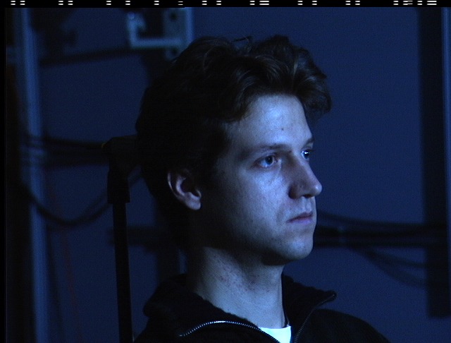
	1.04
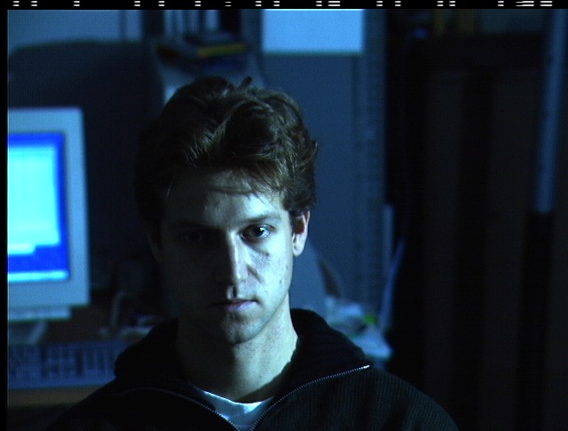
1.22		1.33
	0.78
1.33		1.26
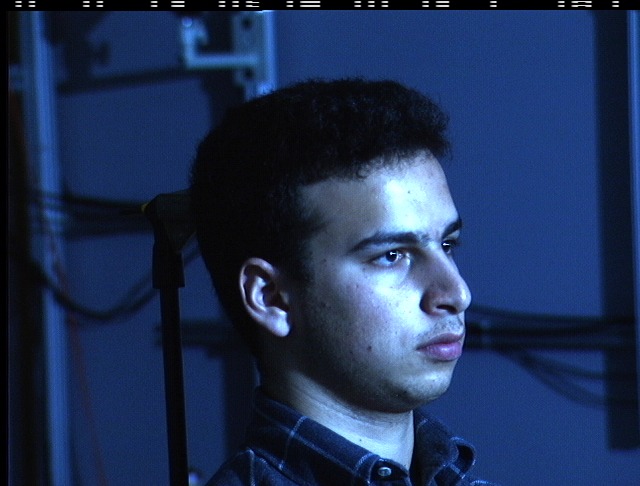
	0.99

Figure 1: Illumination and Pose invariance. Pose and illumination have been a long standing problem in face recognition. This figure shows the output distances of FaceNet between pairs of faces of the same and a different person in different pose and illumination combinations. A distance of $0.0$ means the faces are identical, $4.0$ corresponds to the opposite spectrum, two different identities. You can see that a threshold of 1.1 would classify every pair correctly.

In this paper we present a unified system for face verification (is this the same person), recognition (who is this person) and clustering (find common people among these faces). Our method is based on learning a Euclidean embedding per image using a deep convolutional network. The network is trained such that the squared L2 distances in the embedding space directly correspond to face similarity: faces of the same person have small distances and faces of distinct people have large distances.

Once this embedding has been produced, then the aforementioned tasks become straight-forward: face verification simply involves thresholding the distance between the two embeddings; recognition becomes a k-NN classification problem; and clustering can be achieved using off-the-shelf techniques such as k-means or agglomerative clustering.

Previous face recognition approaches based on deep networks use a classification layer [15, 17] trained over a set of known face identities and then take an intermediate bottleneck layer as a representation used to generalize recognition beyond the set of identities used in training. The downsides of this approach are its indirectness and its inefficiency: one has to hope that the bottleneck representation generalizes well to new faces; and by using a bottleneck layer the representation size per face is usually very large (1000s of dimensions). Some recent work [15] has reduced this dimensionality using PCA, but this is a linear transformation that can be easily learnt in one layer of the network.

In contrast to these approaches, FaceNet directly trains its output to be a compact 128-D embedding using a triplet-based loss function based on LMNN [19]. Our triplets consist of two matching face thumbnails and a non-matching face thumbnail and the loss aims to separate the positive pair from the negative by a distance margin. The thumbnails are tight crops of the face area, no 2D or 3D alignment, other than scale and translation is performed.

Choosing which triplets to use turns out to be very important for achieving good performance and, inspired by curriculum learning [1], we present a novel online negative exemplar mining strategy which ensures consistently increasing difficulty of triplets as the network trains. To improve clustering accuracy, we also explore hard-positive mining techniques which encourage spherical clusters for the embeddings of a single person.

As an illustration of the incredible variability that our method can handle see Figure 1. Shown are image pairs from PIE [13] that previously were considered to be very difficult for face verification systems.

An overview of the rest of the paper is as follows: in section 2 we review the literature in this area; section 3.1 defines the triplet loss and section 3.2 describes our novel triplet selection and training procedure; in section 3.3 we describe the model architecture used. Finally in section 4 and 5 we present some quantitative results of our embeddings and also qualitatively explore some clustering results.

2 Related Work

Similarly to other recent works which employ deep networks [15, 17], our approach is a purely data driven method which learns its representation directly from the pixels of the face. Rather than using engineered features, we use a large dataset of labelled faces to attain the appropriate invariances to pose, illumination, and other variational conditions.

In this paper we explore two different deep network architectures that have been recently used to great success in the computer vision community. Both are deep convolutional networks [8, 11]. The first architecture is based on the Zeiler&Fergus [22] model which consists of multiple interleaved layers of convolutions, non-linear activations, local response normalizations, and max pooling layers. We additionally add several $1{\times}1{\times}d$ convolution layers inspired by the work of [9]. The second architecture is based on the Inception model of Szegedy et al. which was recently used as the winning approach for ImageNet 2014 [16]. These networks use mixed layers that run several different convolutional and pooling layers in parallel and concatenate their responses. We have found that these models can reduce the number of parameters by up to 20 times and have the potential to reduce the number of FLOPS required for comparable performance.

There is a vast corpus of face verification and recognition works. Reviewing it is out of the scope of this paper so we will only briefly discuss the most relevant recent work.

The works of [15, 17, 23] all employ a complex system of multiple stages, that combines the output of a deep convolutional network with PCA for dimensionality reduction and an SVM for classification.

Zhenyao et al. [23] employ a deep network to “warp” faces into a canonical frontal view and then learn CNN that classifies each face as belonging to a known identity. For face verification, PCA on the network output in conjunction with an ensemble of SVMs is used.

Taigman et al. [17] propose a multi-stage approach that aligns faces to a general 3D shape model. A multi-class network is trained to perform the face recognition task on over four thousand identities. The authors also experimented with a so called Siamese network where they directly optimize the $L_{1}$-distance between two face features. Their best performance on LFW ($97.35\%$) stems from an ensemble of three networks using different alignments and color channels. The predicted distances (non-linear SVM predictions based on the $\chi^{2}$ kernel) of those networks are combined using a non-linear SVM.

Sun et al. [14, 15] propose a compact and therefore relatively cheap to compute network. They use an ensemble of 25 of these network, each operating on a different face patch. For their final performance on LFW ($99.47\%$ [15]) the authors combine 50 responses (regular and flipped). Both PCA and a Joint Bayesian model [2] that effectively correspond to a linear transform in the embedding space are employed. Their method does not require explicit 2D/3D alignment. The networks are trained by using a combination of classification and verification loss. The verification loss is similar to the triplet loss we employ [12, 19], in that it minimizes the $L_{2}$-distance between faces of the same identity and enforces a margin between the distance of faces of different identities. The main difference is that only pairs of images are compared, whereas the triplet loss encourages a relative distance constraint.

A similar loss to the one used here was explored in Wang et al. [18] for ranking images by semantic and visual similarity.

3 Method

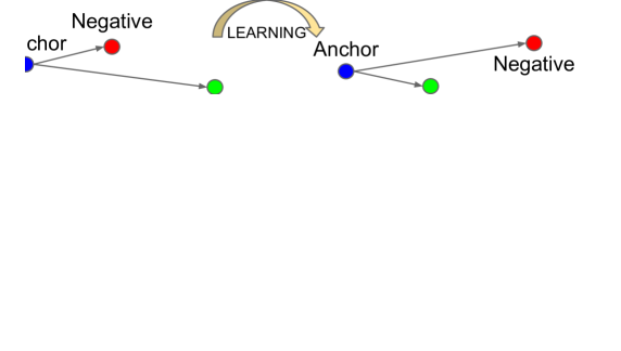
Figure 2: Model structure. Our network consists of a batch input layer and a deep CNN followed by $L_{2}$ normalization, which results in the face embedding. This is followed by the triplet loss during training.

FaceNet uses a deep convolutional network. We discuss two different core architectures: The Zeiler&Fergus [22] style networks and the recent Inception [16] type networks. The details of these networks are described in section 3.3.

Given the model details, and treating it as a black box (see Figure 2), the most important part of our approach lies in the end-to-end learning of the whole system. To this end we employ the triplet loss that directly reflects what we want to achieve in face verification, recognition and clustering. Namely, we strive for an embedding $f(x)$, from an image $x$ into a feature space $\mathbb{R}^{d}$, such that the squared distance between all faces, independent of imaging conditions, of the same identity is small, whereas the squared distance between a pair of face images from different identities is large.

Although we did not directly compare to other losses, e.g. the one using pairs of positives and negatives, as used in [14] Eq. (2), we believe that the triplet loss is more suitable for face verification. The motivation is that the loss from [14] encourages all faces of one identity to be projected onto a single point in the embedding space. The triplet loss, however, tries to enforce a margin between each pair of faces from one person to all other faces. This allows the faces for one identity to live on a manifold, while still enforcing the distance and thus discriminability to other identities.

The following section describes this triplet loss and how it can be learned efficiently at scale.

3.1 Triplet Loss

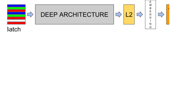
Figure 3: The Triplet Loss minimizes the distance between an anchor and a positive, both of which have the same identity, and maximizes the distance between the anchor and a negative of a different identity.

The embedding is represented by $f(x)\in\mathbb{R}^{d}$. It embeds an image $x$ into a $d$-dimensional Euclidean space. Additionally, we constrain this embedding to live on the $d$-dimensional hypersphere, i.e. $\|f(x)\|_{2}=1$. This loss is motivated in [19] in the context of nearest-neighbor classification. Here we want to ensure that an image $x_{i}^{a}$ (anchor) of a specific person is closer to all other images $x_{i}^{p}$ (positive) of the same person than it is to any image $x_{i}^{n}$ (negative) of any other person. This is visualized in Figure 3.

Thus we want,

$$\|f(x_{i}^{a})-f(x_{i}^{p})\|_{2}^{2}+\alpha <\|f(x_{i}^{a})-f(x_{i}^{n})\|_{2}^{2}\;,$$ (1)

$$\>\forall\left(f(x_{i}^{a}),f(x_{i}^{p}),f(x_{i}^{n})\right)\in\mathcal{T}\;.$$ (2)

where $\alpha$ is a margin that is enforced between positive and negative pairs. $\mathcal{T}$ is the set of all possible triplets in the training set and has cardinality $N$.

The loss that is being minimized is then $L=$

$$\sum_{i}^{N}\left[\left\|f(x_{i}^{a})-f(x_{i}^{p})\right\|_{2}^{2}-\left\|f(x_{i}^{a})-f(x_{i}^{n})\right\|_{2}^{2}+\alpha\right]_{+}\;.$$ (3)

Generating all possible triplets would result in many triplets that are easily satisfied (i.e. fulfill the constraint in Eq. (1)). These triplets would not contribute to the training and result in slower convergence, as they would still be passed through the network. It is crucial to select hard triplets, that are active and can therefore contribute to improving the model. The following section talks about the different approaches we use for the triplet selection.

3.2 Triplet Selection

In order to ensure fast convergence it is crucial to select triplets that violate the triplet constraint in Eq. (1). This means that, given $x_{i}^{a}$, we want to select an $x_{i}^{p}$ (hard positive) such that $\operatorname{argmax}_{x_{i}^{p}}\left\|f(x_{i}^{a})-f(x_{i}^{p})\right\|_{2}^{2}$ and similarly $x_{i}^{n}$ (hard negative) such that $\operatorname{argmin}_{x_{i}^{n}}\left\|f(x_{i}^{a})-f(x_{i}^{n})\right\|_{2}^{2}$.

It is infeasible to compute the $\operatorname{argmin}$ and $\operatorname{argmax}$ across the whole training set. Additionally, it might lead to poor training, as mislabelled and poorly imaged faces would dominate the hard positives and negatives. There are two obvious choices that avoid this issue:

• Generate triplets offline every n steps, using the most recent network checkpoint and computing the $\operatorname{argmin}$ and $\operatorname{argmax}$ on a subset of the data.

• Generate triplets online. This can be done by selecting the hard positive/negative exemplars from within a mini-batch.

Here, we focus on the online generation and use large mini-batches in the order of a few thousand exemplars and only compute the $\operatorname{argmin}$ and $\operatorname{argmax}$ within a mini-batch.

To have a meaningful representation of the anchor-positive distances, it needs to be ensured that a minimal number of exemplars of any one identity is present in each mini-batch. In our experiments we sample the training data such that around 40 faces are selected per identity per mini-batch. Additionally, randomly sampled negative faces are added to each mini-batch.

Instead of picking the hardest positive, we use all anchor-positive pairs in a mini-batch while still selecting the hard negatives. We don’t have a side-by-side comparison of hard anchor-positive pairs versus all anchor-positive pairs within a mini-batch, but we found in practice that the all anchor-positive method was more stable and converged slightly faster at the beginning of training.

We also explored the offline generation of triplets in conjunction with the online generation and it may allow the use of smaller batch sizes, but the experiments were inconclusive.

Selecting the hardest negatives can in practice lead to bad local minima early on in training, specifically it can result in a collapsed model (i.e. $f(x)=0$). In order to mitigate this, it helps to select $x_{i}^{n}$ such that

$$\left\|f(x_{i}^{a})-f(x_{i}^{p})\right\|_{2}^{2}<\left\|f(x_{i}^{a})-f(x_{i}^{n})\right\|_{2}^{2}\;.$$ (4)

We call these negative exemplars semi-hard, as they are further away from the anchor than the positive exemplar, but still hard because the squared distance is close to the anchor-positive distance. Those negatives lie inside the margin $\alpha$.

As mentioned before, correct triplet selection is crucial for fast convergence. On the one hand we would like to use small mini-batches as these tend to improve convergence during Stochastic Gradient Descent (SGD) [20]. On the other hand, implementation details make batches of tens to hundreds of exemplars more efficient. The main constraint with regards to the batch size, however, is the way we select hard relevant triplets from within the mini-batches. In most experiments we use a batch size of around 1,800 exemplars.

3.3 Deep Convolutional Networks

layer	size-in	size-out	kernel	param	FLPS
conv1	$220{\times}220{\times}3$	$110{\times}110{\times}64$	$7{\times}7{\times}3,2$	9K	115M
pool1	$110{\times}110{\times}64$	$55{\times}55{\times}64$	$3{\times}3{\times}64,2$	0
rnorm1	$55{\times}55{\times}64$	$55{\times}55{\times}64$		0
conv2a	$55{\times}55{\times}64$	$55{\times}55{\times}64$	$1{\times}1{\times}64,1$	4K	13M
conv2	$55{\times}55{\times}64$	$55{\times}55{\times}192$	$3{\times}3{\times}64,1$	111K	335M
rnorm2	$55{\times}55{\times}192$	$55{\times}55{\times}192$		0
pool2	$55{\times}55{\times}192$	$28{\times}28{\times}192$	$3{\times}3{\times}192,2$	0
conv3a	$28{\times}28{\times}192$	$28{\times}28{\times}192$	$1{\times}1{\times}192,1$	37K	29M
conv3	$28{\times}28{\times}192$	$28{\times}28{\times}384$	$3{\times}3{\times}192,1$	664K	521M
pool3	$28{\times}28{\times}384$	$14{\times}14{\times}384$	$3{\times}3{\times}384,2$	0
conv4a	$14{\times}14{\times}384$	$14{\times}14{\times}384$	$1{\times}1{\times}384,1$	148K	29M
conv4	$14{\times}14{\times}384$	$14{\times}14{\times}256$	$3{\times}3{\times}384,1$	885K	173M
conv5a	$14{\times}14{\times}256$	$14{\times}14{\times}256$	$1{\times}1{\times}256,1$	66K	13M
conv5	$14{\times}14{\times}256$	$14{\times}14{\times}256$	$3{\times}3{\times}256,1$	590K	116M
conv6a	$14{\times}14{\times}256$	$14{\times}14{\times}256$	$1{\times}1{\times}256,1$	66K	13M
conv6	$14{\times}14{\times}256$	$14{\times}14{\times}256$	$3{\times}3{\times}256,1$	590K	116M
pool4	$14{\times}14{\times}256$	$7{\times}7{\times}256$	$3{\times}3{\times}256,2$	0
concat	$7{\times}7{\times}256$	$7{\times}7{\times}256$		0
fc1	$7{\times}7{\times}256$	$1{\times}32{\times}128$	maxout p=2	103M	103M
fc2	$1{\times}32{\times}128$	$1{\times}32{\times}128$	maxout p=2	34M	34M
fc7128	$1{\times}32{\times}128$	$1{\times}1{\times}128$		524K	0.5M
L2	$1{\times}1{\times}128$	$1{\times}1{\times}128$		0
total				140M	1.6B

Table 1: NN1. This table show the structure of our Zeiler&Fergus [22] based model with $1{\times}1$ convolutions inspired by [9]. The input and output sizes are described in $rows\times cols\times\#filters$. The kernel is specified as $rows\times cols,stride$ and the maxout [6] pooling size as $p=2$.

In all our experiments we train the CNN using Stochastic Gradient Descent (SGD) with standard backprop [8, 11] and AdaGrad [5]. In most experiments we start with a learning rate of $0.05$ which we lower to finalize the model. The models are initialized from random, similar to [16], and trained on a CPU cluster for 1,000 to 2,000 hours. The decrease in the loss (and increase in accuracy) slows down drastically after 500h of training, but additional training can still significantly improve performance. The margin $\alpha$ is set to $0.2$.

We used two types of architectures and explore their trade-offs in more detail in the experimental section. Their practical differences lie in the difference of parameters and FLOPS. The best model may be different depending on the application. E.g. a model running in a datacenter can have many parameters and require a large number of FLOPS, whereas a model running on a mobile phone needs to have few parameters, so that it can fit into memory. All our models use rectified linear units as the non-linear activation function.

The first category, shown in Table 1, adds $1{\times}1{\times}d$ convolutional layers, as suggested in [9], between the standard convolutional layers of the Zeiler&Fergus [22] architecture and results in a model 22 layers deep. It has a total of 140 million parameters and requires around 1.6 billion FLOPS per image.

The second category we use is based on GoogLeNet style Inception models [16]. These models have $20{\times}$ fewer parameters (around 6.6M-7.5M) and up to $5{\times}$ fewer FLOPS (between 500M-1.6B). Some of these models are dramatically reduced in size (both depth and number of filters), so that they can be run on a mobile phone. One, NNS1, has 26M parameters and only requires 220M FLOPS per image. The other, NNS2, has 4.3M parameters and 20M FLOPS. Table 2 describes NN2 our largest network in detail. NN3 is identical in architecture but has a reduced input size of 160x160. NN4 has an input size of only 96x96, thereby drastically reducing the CPU requirements (285M FLOPS vs 1.6B for NN2). In addition to the reduced input size it does not use 5x5 convolutions in the higher layers as the receptive field is already too small by then. Generally we found that the 5x5 convolutions can be removed throughout with only a minor drop in accuracy. Figure 4 compares all our models.

type	output     size	depth	$\#1{\times}1$	$\#3{\times}3$    reduce	$\#3{\times}3$	$\#5{\times}5$    reduce	$\#5{\times}5$	pool   proj (p)	params	FLOPS
conv1 ($7{\times}7{\times}3,2$)	$112{\times}112{\times}64$	1							9K	119M
max pool + norm	$56{\times}56{\times}64$	0						m $3{\times}3,2$
inception (2)	$56{\times}56{\times}192$	2		64	192				115K	360M
norm + max pool	$28{\times}28{\times}192$	0						m $3{\times}3,2$
inception (3a)	$28{\times}28{\times}256$	2	64	96	128	16	32	m, 32p	164K	128M
inception (3b)	$28{\times}28{\times}320$	2	64	96	128	32	64	$L_{2}$, 64p	228K	179M
inception (3c)	$14{\times}14{\times}640$	2	0	128	256,2	32	64,2	m $3{\times}3$,2	398K	108M
inception (4a)	$14{\times}14{\times}640$	2	256	96	192	32	64	$L_{2}$, 128p	545K	107M
inception (4b)	$14{\times}14{\times}640$	2	224	112	224	32	64	$L_{2}$, 128p	595K	117M
inception (4c)	$14{\times}14{\times}640$	2	192	128	256	32	64	$L_{2}$, 128p	654K	128M
inception (4d)	$14{\times}14{\times}640$	2	160	144	288	32	64	$L_{2}$, 128p	722K	142M
inception (4e)	$7{\times}7{\times}1024$	2	0	160	256,2	64	128,2	m $3{\times}3$,2	717K	56M
inception (5a)	$7{\times}7{\times}1024$	2	384	192	384	48	128	$L_{2}$, 128p	1.6M	78M
inception (5b)	$7{\times}7{\times}1024$	2	384	192	384	48	128	m, 128p	1.6M	78M
avg pool	$1{\times}1{\times}1024$	0
fully conn	$1{\times}1{\times}128$	1							131K	0.1M
L2 normalization	$1{\times}1{\times}128$	0
total									7.5M	1.6B

Table 2: NN2. Details of the NN2 Inception incarnation. This model is almost identical to the one described in  [16]. The two major differences are the use of $L_{2}$ pooling instead of max pooling (m), where specified. I.e. instead of taking the spatial max the $L_{2}$ norm is computed. The pooling is always $3{\times}3$ (aside from the final average pooling) and in parallel to the convolutional modules inside each Inception module. If there is a dimensionality reduction after the pooling it is denoted with p. $1{\times}1$, $3{\times}3$, and $5{\times}5$ pooling are then concatenated to get the final output.

4 Datasets and Evaluation

We evaluate our method on four datasets and with the exception of Labelled Faces in the Wild and YouTube Faces we evaluate our method on the face verification task. I.e. given a pair of two face images a squared $L_{2}$ distance threshold $D(x_{i},x_{j})$ is used to determine the classification of same and different. All faces pairs $(i,j)$ of the same identity are denoted with $\mathcal{P_{\text{same}}}$, whereas all pairs of different identities are denoted with $\mathcal{P_{\text{diff}}}$.

We define the set of all true accepts as

$$\operatorname{TA}(d)=\{(i,j)\in\mathcal{P_{\text{same}}},\text{with}\,D(x_{i},x_{j})\leq d\}\;.$$ (5)

These are the face pairs $(i,j)$ that were correctly classified as same at threshold $d$. Similarly

$$\operatorname{FA}(d)=\{(i,j)\in\mathcal{P_{\text{diff}}},\text{with}\,D(x_{i},x_{j})\leq d\}$$ (6)

is the set of all pairs that was incorrectly classified as same (false accept).

The validation rate $\operatorname{VAL}(d)$ and the false accept rate $\operatorname{FAR}(d)$ for a given face distance $d$ are then defined as

$$\operatorname{VAL}(d)=\frac{\left|\operatorname{TA}(d)\right|}{\left|\mathcal{P_{\text{same}}}\right|}\;,\quad\operatorname{FAR}(d)=\frac{\left|\operatorname{FA}(d)\right|}{\left|\mathcal{P_{\text{diff}}}\right|}\;.$$ (7)

4.1 Hold-out Test Set

We keep a hold out set of around one million images, that has the same distribution as our training set, but disjoint identities. For evaluation we split it into five disjoint sets of $200\text{k}$ images each. The $\operatorname{FAR}$ and $\operatorname{VAL}$ rate are then computed on $100\text{k}\times 100\text{k}$ image pairs. Standard error is reported across the five splits.

4.2 Personal Photos

This is a test set with similar distribution to our training set, but has been manually verified to have very clean labels. It consists of three personal photo collections with a total of around $12\text{k}$ images. We compute the $\operatorname{FAR}$ and $\operatorname{VAL}$ rate across all 12k squared pairs of images.

4.3 Academic Datasets

Labeled Faces in the Wild (LFW) is the de-facto academic test set for face verification [7]. We follow the standard protocol for unrestricted, labeled outside data and report the mean classification accuracy as well as the standard error of the mean.

Youtube Faces DB [21] is a new dataset that has gained popularity in the face recognition community [17, 15]. The setup is similar to LFW, but instead of verifying pairs of images, pairs of videos are used.

5 Experiments

If not mentioned otherwise we use between 100M-200M training face thumbnails consisting of about 8M different identities. A face detector is run on each image and a tight bounding box around each face is generated. These face thumbnails are resized to the input size of the respective network. Input sizes range from 96x96 pixels to 224x224 pixels in our experiments.

5.1 Computation Accuracy Trade-off

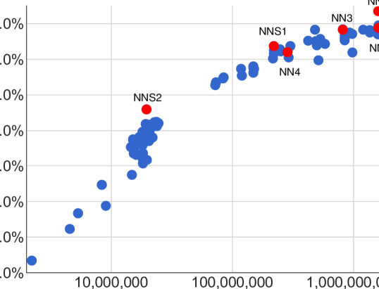
Figure 4: FLOPS vs. Accuracy trade-off. Shown is the trade-off between FLOPS and accuracy for a wide range of different model sizes and architectures. Highlighted are the four models that we focus on in our experiments.

Before diving into the details of more specific experiments we will discuss the trade-off of accuracy versus number of FLOPS that a particular model requires. Figure 4 shows the FLOPS on the x-axis and the accuracy at 0.001 false accept rate ($\operatorname{FAR}$) on our user labelled test-data set from section 4.2. It is interesting to see the strong correlation between the computation a model requires and the accuracy it achieves. The figure highlights the five models (NN1, NN2, NN3, NNS1, NNS2) that we discuss in more detail in our experiments.

We also looked into the accuracy trade-off with regards to the number of model parameters. However, the picture is not as clear in that case. For example, the Inception based model NN2 achieves a comparable performance to NN1, but only has a 20th of the parameters. The number of FLOPS is comparable, though. Obviously at some point the performance is expected to decrease, if the number of parameters is reduced further. Other model architectures may allow further reductions without loss of accuracy, just like Inception [16] did in this case.

5.2 Effect of CNN Model

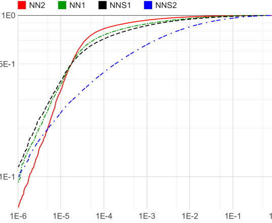
Figure 5: Network Architectures. This plot shows the complete ROC for the four different models on our personal photos test set from section 4.2. The sharp drop at $10\text{\sc{e}-4}$ $\operatorname{FAR}$ can be explained by noise in the groundtruth labels. The models in order of performance are: NN2: $224{\times}224$ input Inception based model; NN1: Zeiler&Fergus based network with $1{\times}1$ convolutions; NNS1: small Inception style model with only 220M FLOPS; NNS2: tiny Inception model with only 20M FLOPS.

architecture	$\operatorname{VAL}$
NN1 (Zeiler&Fergus $220{\times}220$)	$87.9\%\pm 1.9$
NN2 (Inception $224{\times}224$)	$89.4\%\pm 1.6$
NN3 (Inception $160{\times}160$)	$88.3\%\pm 1.7$
NN4 (Inception $96{\times}96$)	$82.0\%\pm 2.3$
NNS1 (mini Inception $165{\times}165$)	$82.4\%\pm 2.4$
NNS2 (tiny Inception $140{\times}116$)	$51.9\%\pm 2.9$

Table 3: Network Architectures. This table compares the performance of our model architectures on the hold out test set (see section 4.1). Reported is the mean validation rate $\operatorname{VAL}$ at $10\text{\sc{e}-3}$ false accept rate. Also shown is the standard error of the mean across the five test splits.

We now discuss the performance of our four selected models in more detail. On the one hand we have our traditional Zeiler&Fergus based architecture with $1{\times}1$ convolutions [22, 9] (see Table 1). On the other hand we have Inception [16] based models that dramatically reduce the model size. Overall, in the final performance the top models of both architectures perform comparably. However, some of our Inception based models, such as NN3, still achieve good performance while significantly reducing both the FLOPS and the model size.

The detailed evaluation on our personal photos test set is shown in Figure 5. While the largest model achieves a dramatic improvement in accuracy compared to the tiny NNS2, the latter can be run 30ms / image on a mobile phone and is still accurate enough to be used in face clustering. The sharp drop in the ROC for $\operatorname{FAR}<10^{-4}$ indicates noisy labels in the test data groundtruth. At extremely low false accept rates a single mislabeled image can have a significant impact on the curve.

5.3 Sensitivity to Image Quality

jpeg q	val-rate
10	67.3%
20	81.4%
30	83.9%
50	85.5%
70	86.1%
90	86.5%

#pixels	val-rate
1,600	37.8%
6,400	79.5%
14,400	84.5%
25,600	85.7%
65,536	86.4%

Table 4: Image Quality. The table on the left shows the effect on the validation rate at $10\text{\sc{e}-3}$ precision with varying JPEG quality. The one on the right shows how the image size in pixels effects the validation rate at $10\text{\sc{e}-3}$ precision. This experiment was done with NN1 on the first split of our test hold-out dataset.

Table 4 shows the robustness of our model across a wide range of image sizes. The network is surprisingly robust with respect to JPEG compression and performs very well down to a JPEG quality of 20. The performance drop is very small for face thumbnails down to a size of 120x120 pixels and even at 80x80 pixels it shows acceptable performance. This is notable, because the network was trained on 220x220 input images. Training with lower resolution faces could improve this range further.

5.4 Embedding Dimensionality

#dims	$\operatorname{VAL}$
64	$86.8\%\pm 1.7$
128	$87.9\%\pm 1.9$
256	$87.7\%\pm 1.9$
512	$85.6\%\pm 2.0$

Table 5: Embedding Dimensionality. This Table compares the effect of the embedding dimensionality of our model NN1 on our hold-out set from section 4.1. In addition to the $\operatorname{VAL}$ at $10\text{\sc{e}-3}$ we also show the standard error of the mean computed across five splits.

We explored various embedding dimensionalities and selected 128 for all experiments other than the comparison reported in Table 5. One would expect the larger embeddings to perform at least as good as the smaller ones, however, it is possible that they require more training to achieve the same accuracy. That said, the differences in the performance reported in Table 5 are statistically insignificant.

It should be noted, that during training a 128 dimensional float vector is used, but it can be quantized to 128-bytes without loss of accuracy. Thus each face is compactly represented by a 128 dimensional byte vector, which is ideal for large scale clustering and recognition. Smaller embeddings are possible at a minor loss of accuracy and could be employed on mobile devices.

5.5 Amount of Training Data

#training images	$\operatorname{VAL}$
2,600,000	76.3%
26,000,000	85.1%
52,000,000	85.1%
260,000,000	86.2%

Table 6: Training Data Size. This table compares the performance after 700h of training for a smaller model with 96x96 pixel inputs. The model architecture is similar to NN2, but without the 5x5 convolutions in the Inception modules.

Table 6 shows the impact of large amounts of training data. Due to time constraints this evaluation was run on a smaller model; the effect may be even larger on larger models. It is clear that using tens of millions of exemplars results in a clear boost of accuracy on our personal photo test set from section 4.2. Compared to only millions of images the relative reduction in error is 60%. Using another order of magnitude more images (hundreds of millions) still gives a small boost, but the improvement tapers off.

5.6 Performance on LFW

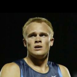
False accept False reject

Figure 6: LFW errors. This shows all pairs of images that were incorrectly classified on LFW. Only eight of the 13 false rejects shown here are actual errors the other five are mislabeled in LFW.

We evaluate our model on LFW using the standard protocol for unrestricted, labeled outside data. Nine training splits are used to select the $L_{2}$-distance threshold. Classification (same or different) is then performed on the tenth test split. The selected optimal threshold is $1.242$ for all test splits except split eighth ($1.256$).

Our model is evaluated in two modes:

1. Fixed center crop of the LFW provided thumbnail.

2. A proprietary face detector (similar to Picasa [3]) is run on the provided LFW thumbnails. If it fails to align the face (this happens for two images), the LFW alignment is used.

Figure 6 gives an overview of all failure cases. It shows false accepts on the top as well as false rejects at the bottom. We achieve a classification accuracy of 98.87%$\pm 0.15$ when using the fixed center crop described in (1) and the record breaking 99.63%$\pm$0.09 standard error of the mean when using the extra face alignment (2). This reduces the error reported for DeepFace in [17] by more than a factor of 7 and the previous state-of-the-art reported for DeepId2+ in [15] by 30%. This is the performance of model NN1, but even the much smaller NN3 achieves performance that is not statistically significantly different.

5.7 Performance on Youtube Faces DB

We use the average similarity of all pairs of the first one hundred frames that our face detector detects in each video. This gives us a classification accuracy of 95.12%$\pm 0.39$. Using the first one thousand frames results in 95.18%. Compared to [17] 91.4% who also evaluate one hundred frames per video we reduce the error rate by almost half. DeepId2+ [15] achieved 93.2% and our method reduces this error by 30%, comparable to our improvement on LFW.

5.8 Face Clustering

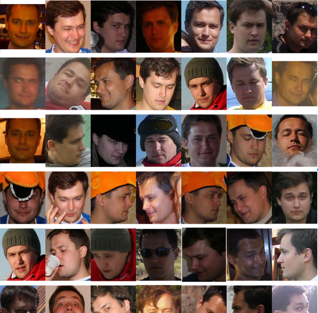
Figure 7: Face Clustering. Shown is an exemplar cluster for one user. All these images in the users personal photo collection were clustered together.

Our compact embedding lends itself to be used in order to cluster a users personal photos into groups of people with the same identity. The constraints in assignment imposed by clustering faces, compared to the pure verification task, lead to truly amazing results. Figure 7 shows one cluster in a users personal photo collection, generated using agglomerative clustering. It is a clear showcase of the incredible invariance to occlusion, lighting, pose and even age.

6 Summary

We provide a method to directly learn an embedding into an Euclidean space for face verification. This sets it apart from other methods [15, 17] who use the CNN bottleneck layer, or require additional post-processing such as concatenation of multiple models and PCA, as well as SVM classification. Our end-to-end training both simplifies the setup and shows that directly optimizing a loss relevant to the task at hand improves performance.

Another strength of our model is that it only requires minimal alignment (tight crop around the face area). [17], for example, performs a complex 3D alignment. We also experimented with a similarity transform alignment and notice that this can actually improve performance slightly. It is not clear if it is worth the extra complexity.

Future work will focus on better understanding of the error cases, further improving the model, and also reducing model size and reducing CPU requirements. We will also look into ways of improving the currently extremely long training times, e.g. variations of our curriculum learning with smaller batch sizes and offline as well as online positive and negative mining.

7 Appendix: Harmonic Embedding

In this section we introduce the concept of harmonic embeddings. By this we denote a set of embeddings that are generated by different models v1 and v2 but are compatible in the sense that they can be compared to each other.

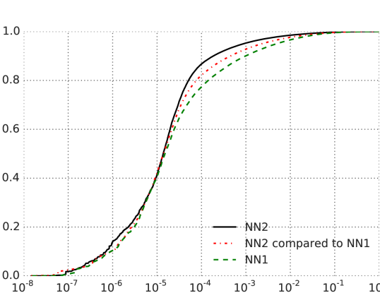
Figure 8: Harmonic Embedding Compatibility. These ROCs show the compatibility of the harmonic embeddings of NN2 to the embeddings of NN1. NN2 is an improved model that performs much better than NN1. When comparing embeddings generated by NN1 to the harmonic ones generated by NN2 we can see the compatibility between the two. In fact, the mixed mode performance is still better than NN1 by itself.

This compatibility greatly simplifies upgrade paths. E.g. in an scenario where embedding v1 was computed across a large set of images and a new embedding model v2 is being rolled out, this compatibility ensures a smooth transition without the need to worry about version incompatibilities. Figure 8 shows results on our 3G dataset. It can be seen that the improved model NN2 significantly outperforms NN1, while the comparison of NN2 embeddings to NN1 embeddings performs at an intermediate level.

7.1 Harmonic Triplet Loss

Figure 9: Learning the Harmonic Embedding. In order to learn a harmonic embedding, we generate triplets that mix the v1 embeddings with the v2 embeddings that are being trained. The semi-hard negatives are selected from the whole set of both v1 and v2 embeddings.

In order to learn the harmonic embedding we mix embeddings of v1 together with the embeddings v2, that are being learned. This is done inside the triplet loss and results in additionally generated triplets that encourage the compatibility between the different embedding versions. Figure 9 visualizes the different combinations of triplets that contribute to the triplet loss.

We initialized the v2 embedding from an independently trained NN2 and retrained the last layer (embedding layer) from random initialization with the compatibility encouraging triplet loss. First only the last layer is retrained, then we continue training the whole v2 network with the harmonic loss.

Figure 10 shows a possible interpretation of how this compatibility may work in practice. The vast majority of v2 embeddings may be embedded near the corresponding v1 embedding, however, incorrectly placed v1 embeddings can be perturbed slightly such that their new location in embedding space improves verification accuracy.

7.2 Summary

These are very interesting findings and it is somewhat surprising that it works so well. Future work can explore how far this idea can be extended. Presumably there is a limit as to how much the v2 embedding can improve over v1, while still being compatible. Additionally it would be interesting to train small networks that can run on a mobile phone and are compatible to a larger server side model.

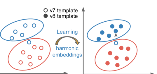
Figure 10: Harmonic Embedding Space. This visualisation sketches a possible interpretation of how harmonic embeddings are able to improve verification accuracy while maintaining compatibility to less accurate embeddings. In this scenario there is one misclassified face, whose embedding is perturbed to the “correct” location in v2.

References

- [1] Y. Bengio, J. Louradour, R. Collobert, and J. Weston. Curriculum learning. In Proc. of ICML, New York, NY, USA, 2009.
- [2] D. Chen, X. Cao, L. Wang, F. Wen, and J. Sun. Bayesian face revisited: A joint formulation. In Proc. ECCV, 2012.
- [3] D. Chen, S. Ren, Y. Wei, X. Cao, and J. Sun. Joint cascade face detection and alignment. In Proc. ECCV, 2014.
- [4] J. Dean, G. Corrado, R. Monga, K. Chen, M. Devin, M. Mao, M. Ranzato, A. Senior, P. Tucker, K. Yang, Q. V. Le, and A. Y. Ng. Large scale distributed deep networks. In P. Bartlett, F. Pereira, C. Burges, L. Bottou, and K. Weinberger, editors, NIPS, pages 1232–1240. 2012.
- [5] J. Duchi, E. Hazan, and Y. Singer. Adaptive subgradient methods for online learning and stochastic optimization. J. Mach. Learn. Res., 12:2121–2159, July 2011.
- [6] I. J. Goodfellow, D. Warde-farley, M. Mirza, A. Courville, and Y. Bengio. Maxout networks. In In ICML, 2013.
- [7] G. B. Huang, M. Ramesh, T. Berg, and E. Learned-Miller. Labeled faces in the wild: A database for studying face recognition in unconstrained environments. Technical Report 07-49, University of Massachusetts, Amherst, October 2007.
- [8] Y. LeCun, B. Boser, J. S. Denker, D. Henderson, R. E. Howard, W. Hubbard, and L. D. Jackel. Backpropagation applied to handwritten zip code recognition. Neural Computation, 1(4):541–551, Dec. 1989.
- [9] M. Lin, Q. Chen, and S. Yan. Network in network. CoRR, abs/1312.4400, 2013.
- [10] C. Lu and X. Tang. Surpassing human-level face verification performance on LFW with gaussianface. CoRR, abs/1404.3840, 2014.
- [11] D. E. Rumelhart, G. E. Hinton, and R. J. Williams. Learning representations by back-propagating errors. Nature, 1986.
- [12] M. Schultz and T. Joachims. Learning a distance metric from relative comparisons. In S. Thrun, L. Saul, and B. Schölkopf, editors, NIPS, pages 41–48. MIT Press, 2004.
- [13] T. Sim, S. Baker, and M. Bsat. The CMU pose, illumination, and expression (PIE) database. In In Proc. FG, 2002.
- [14] Y. Sun, X. Wang, and X. Tang. Deep learning face representation by joint identification-verification. CoRR, abs/1406.4773, 2014.
- [15] Y. Sun, X. Wang, and X. Tang. Deeply learned face representations are sparse, selective, and robust. CoRR, abs/1412.1265, 2014.
- [16] C. Szegedy, W. Liu, Y. Jia, P. Sermanet, S. Reed, D. Anguelov, D. Erhan, V. Vanhoucke, and A. Rabinovich. Going deeper with convolutions. CoRR, abs/1409.4842, 2014.
- [17] Y. Taigman, M. Yang, M. Ranzato, and L. Wolf. Deepface: Closing the gap to human-level performance in face verification. In IEEE Conf. on CVPR, 2014.
- [18] J. Wang, Y. Song, T. Leung, C. Rosenberg, J. Wang, J. Philbin, B. Chen, and Y. Wu. Learning fine-grained image similarity with deep ranking. CoRR, abs/1404.4661, 2014.
- [19] K. Q. Weinberger, J. Blitzer, and L. K. Saul. Distance metric learning for large margin nearest neighbor classification. In NIPS. MIT Press, 2006.
- [20] D. R. Wilson and T. R. Martinez. The general inefficiency of batch training for gradient descent learning. Neural Networks, 16(10):1429–1451, 2003.
- [21] L. Wolf, T. Hassner, and I. Maoz. Face recognition in unconstrained videos with matched background similarity. In IEEE Conf. on CVPR, 2011.
- [22] M. D. Zeiler and R. Fergus. Visualizing and understanding convolutional networks. CoRR, abs/1311.2901, 2013.
- [23] Z. Zhu, P. Luo, X. Wang, and X. Tang. Recover canonical-view faces in the wild with deep neural networks. CoRR, abs/1404.3543, 2014.