An Online Parallel and Distributed Algorithm for Recursive Estimation of Sparse Signals

Abstract

In this paper, we consider a recursive estimation problem for linear regression where the signal to be estimated admits a sparse representation and measurement samples are only sequentially available. We propose a convergent parallel estimation scheme that consists in solving a sequence of $\ell_{1}$-regularized least-square problems approximately. The proposed scheme is novel in three aspects: i) all elements of the unknown vector variable are updated in parallel at each time instance, and convergence speed is much faster than state-of-the-art schemes which update the elements sequentially; ii) both the update direction and stepsize of each element have simple closed-form expressions, so the algorithm is suitable for online (real-time) implementation; and iii) the stepsize is designed to accelerate the convergence but it does not suffer from the common trouble of parameter tuning in literature. Both centralized and distributed implementation schemes are discussed. The attractive features of the proposed algorithm are also numerically consolidated.

I Introduction

Signal estimation has been a fundamental problem in a number of scenarios, such as wireless sensor networks (WSN) and cognitive radio (CR). WSN has received a lot of attention and is found to be useful in diverse disciplines such as environmental monitoring, smart grid, and wireless communications [1]. CR appears as an enabling technique for flexible and efficient use of the radio spectrum [2, 3], since it allows the unlicensed secondary users (SUs) to access the spectrum provided that the licensed primary users (PUs) are idle, and/or the interference generated by the SUs to the PUs is below a certain level that is tolerable for the PUs [4, 5].

One in CR systems is the ability to obtain a precise estimate of the PUs’ power distribution map so that the SUs can avoid the areas in which the PUs are actively transmitting. This is usually realized through the estimation of the position, transmit status, and/or transmit power of PUs [6, 7, 8, 9], and such an estimation is typically obtained based on the minimum mean-square-error (MMSE) criterion [10, 11, 12, 13, 14, 8, 1].

The MMSE approach involves the calculation of the expectation of a squared $\ell_{2}$-norm function that depends on the so-called regression vector and measurement output, both of which are random variables. This is essentially a stochastic optimization problem, but when the statistics of these random variables are unknown, it is impossible to calculate the expectation analytically. An alternative is to use the sample average function, constructed from the sequentially available measurements, as an approximation of the expectation, and this leads to the well-known recursive least-square (RLS) algorithm [11, 12, 13, 1]. As the measurements are available sequentially, at each time instance of the RLS algorithm, an LS problem has to be solved, which furthermore admits a closed-form solution and thus can efficiently be computed. More details can be found in standard textbooks such as [10, 11].

In practice, the signal to be estimated may be sparse in nature [14, 7, 15, 8, 1]. In a recent attempt to apply the RLS approach to estimate a sparse signal, a regularization function in terms of $\ell_{1}$-norm was incorporated into the LS function to encourage sparse estimates [14, 1], leading to an $\ell_{1}$-regularized LS problem which has the form of the least-absolute shrinkage and selection operator (LASSO) [16]. Then in the recursive estimation of a sparse signal, the only difference from standard RLS is that at each time instance, instead of solving an LS problem as in RLS, an $\ell_{1}$-regularized LS problem in the form of LASSO is solved [1].

However, a closed-form solution to the $\ell_{1}$-regularized LS problem no longer exists because of the $\ell_{1}$-norm regularization function and the problem can only be solved iteratively. As a matter of fact, iterative algorithms to solve the $\ell_{1}$-regularized LS problems have been the center of extensive research in recent years and a number of solvers have been developed, e.g., GP [17], l1_ls [18], FISTA [19], ADMM [20], and FLEXA [21]. Since the measurements are sequentially available, and with each measurement, a new $\ell_{1}$-regularized LS problem is formed and solved, the overall complexity of using solvers for the whole sequence of $\ell_{1}$-regularized LS problems is no longer affordable. If the environment is furthermore fast changing, this method is not even real-time applicable because new samples may have already arrived before the old $\ell_{1}$-regularized LS problem is solved.

To make the estimation scheme suitable for online (real-time) implementation, a sequential algorithm was proposed in [14], in which the $\ell_{1}$-regularized LS problem at each time instance is solved only approximately. In particular, at each time instance, the $\ell_{1}$-regularized LS problem is solved with respect to (w.r.t.) only a single element of the unknown vector variable (instead of all elements as in a solver) while remaining elements are fixed, and the element is updated in closed-form based on the so-called soft-thresholding operator [19]. After a new sample arrives, a new $\ell_{1}$-regularized LS problem is formed and solved w.r.t. the next element while remaining elements are fixed. This sequential update rule is known in literature as block coordinate descent method [22]. To our best knowledge, [14] is the only work on online algorithms for recursive estimation of sparse signals.

Intuitively, since only a single element is updated at each time instance, the online algorithm proposed in [14] sometimes suffers from slow convergence, especially when the signal has a large dimension while large dimension of sparse signals is universal in practice. It is tempting to use the parallel algorithm proposed in [23, 21], but it works for deterministic optimization problems only and may not converge for the stochastic optimization problem at hand. Besides, its convergence speed heavily depends on the stepsize. Typical stepsizes are Armijo-like successive line search, constant stepsize, and diminishing stepsize. The former two suffer from high complexity and slow convergence [21, Remark 4], while the decay rate of the diminishing stepsize is very difficult to choose: on the one hand, a slowly decaying stepsize is preferable to make notable progress and to achieve satisfactory convergence speed; on the other hand, theoretical convergence is guaranteed only when the stepsizes decays fast enough. It is a difficult task on its own to find the decay rate that gives a good trade-off.

A recent work on parallel algorithms for stochastic optimization is [24]. However, the algorithms proposed in [24] are not applicable for the recursive estimation of sparse signals. This is because the regularization function in [24] must be strongly convex and differentiable while the regularization gain must be lower bounded by some positive constant so that convergence can be achieved, but the regularization function in terms of $\ell_{1}$-norm in this paper is convex (but not strongly convex) and nonsmooth while the regularization gain is decreasing to 0.

In this paper, we propose an online parallel algorithm with provable convergence for recursive estimation of sparse signals. In particular, our contributions are as follows:

1) At each time instance, the $\ell_{1}$-regularized LS problem is solved approximately and all elements are updated in parallel, so the convergence speed is greatly enhanced compared with [14]. As a nontrivial extension of [14] from sequential update to parallel update and [23, 21] from deterministic optimization problems to stochastic optimization problems, the convergence of the proposed algorithm is established.

2) The proposed stepsize is based on the so-called minimization rule (also known as exact line search) and its benefits are twofold: firstly, it guarantees the convergence of the proposed algorithm, which may however diverge under other stepsize rules; secondly, notable progress is achieved after each variable update and the trouble of parameter tuning in [23, 21] is saved. Besides, both the update direction and stepsize of each element have a simple closed-form expression, so the algorithm is fast to converge and suitable for online implementation.

3) When implemented in a distributed manner, for example in CR networks, the proposed algorithm has a much smaller signaling overhead than in state-of-the-art techniques [1, 7]. Besides, the estimates of different SUs are always the same and they are based on the global information of all SUs. Compared with consensus-based distributed implementations [8, 7, 1] where each SU makes individual estimate decision mainly based on his own local information and all SUs converge to the same estimate only asymptotically, the proposed approach can better protect the Quality-of-Service (QoS) of PUs because it eliminates the possibility that the estimates maintained by different SUs lead to conflicting interests of the PUs (i.e., some may correctly detect the presence of PUs but some may not in consensus-based algorithms).

The rest of the paper is organized as follows. In Section II we introduce the system model and formulate the recursive estimation problem. The online parallel algorithm is proposed in Section III, and its implementations and extensions are discussed in Section IV. The performance of the proposed algorithm is evaluated numerically in Section V and finally concluding remarks are drawn in Section VI.

Notation: We use $x$, $\mathbf{x}$ and $\mathbf{X}$ to denote scalar, vector and matrix, respectively. $X_{jk}$ is the $(j,k)$-th element of $\mathbf{X}$; $x_{k}$ and $x_{j,k}$ is the $k$-th element of $\mathbf{x}$ and $\mathbf{x}_{j}$, respectively, and $\mathbf{x}=(x_{k})_{k=1}^{K}$ and $\mathbf{x}_{j}=(x_{j,k})_{k=1}^{K}$. $\mathbf{d(X)}$ is a vector that consists of the diagonal elements of $\mathbf{X}$. $\mathbf{x}\circ\mathbf{y}$ denotes the Hadamard product between $\mathbf{x}$ and $\mathbf{y}$. $[\mathbf{x}]_{\mathbf{a}}^{\mathbf{b}}$ denotes the element-wise projection of $\mathbf{x}$ onto $[\mathbf{a,b}]$: $[\mathbf{x}]_{\mathbf{a}}^{\mathbf{b}}\triangleq\max(\min(\mathbf{x},\mathbf{b}),\mathbf{a})$, and $\left[\mathbf{x}\right]^{+}$ denotes the element-wise projection of $\mathbf{x}$ onto the nonnegative orthant: $\left[\mathbf{x}\right]^{+}\triangleq\max(\mathbf{x},\mathbf{0})$. $\mathbf{X}^{\dagger}$ denotes the Moore-Penrose inverse of $\mathbf{X}$.

II System Model and Problem Formulation

Suppose $\mathbf{x}^{\star}=(x_{k}^{\star})_{k=1}^{K}\in\mathbb{R}^{K}$ is a deterministic sparse signal to be estimated based on the the measurement $y_{n}\in\mathbb{R}$, and they are connected through a linear regression model:

$$y_{n}=\mathbf{g}_{n}^{T}\mathbf{x}^{\star}+v_{n},\quad n=1,\ldots,N,$$ (1)

where $N$ is the number of measurements at any time instance. The regression vector $\mathbf{g}_{n}=(g_{n,k})_{k=1}^{K}\in\mathbb{R}^{K}$ is assumed to be known, and $v_{n}\in\mathbb{R}$ is the additive estimation noise. Throughout the paper, we make the following assumptions on $\mathbf{g}_{n}$ and $v_{n}$ for $n=1,\ldots,N$:

1. $\mathbf{g}_{n}$ are independently and identically distributed (i.i.d.) random variables with a bounded positive definite covariance matrix;

2. $v_{n}$ are i.i.d. random variables with zero mean and bounded variance, and are uncorrelated with $\mathbf{g}_{n}$.

Given the linear model in (1), the problem is to estimate $\mathbf{x}^{\star}$ from the set of regression vectors and measurements $\left\{\mathbf{g}_{n},y_{n}\right\}_{n=1}^{N}$. Since both the regression vector $\mathbf{g}_{n}$ and estimation noise $v_{n}$ are random variables, the measurement $y_{n}$ is also random. A fundamental approach to estimate $\mathbf{x}^{\star}$ is based on the MMSE criterion, which has a solid root in adaptive filter theory [11, 10]. To improve the estimation precision, all available measurements $\left\{\mathbf{g}_{n},y_{n}\right\}_{n=1}^{N}$ are exploited to form a cooperative estimation problem which consists in finding the variable that minimizes the mean-square-error [25, 1, 8]:

$$\mathbf{x}^{\star} =\underset{\mathbf{x}=(x_{k})_{k=1}^{K}}{\arg\min}\;\mathbb{E}\left[\sum_{n=1}^{N}\left(y_{n}-\mathbf{g}_{n}^{T}\mathbf{x}\right)^{2}\right]$$ (2)

$$=\underset{\mathbf{x}}{\arg\min}\;\frac{1}{2}\mathbf{x}^{T}\mathbf{G}\mathbf{x}-\mathbf{b}^{T}\mathbf{x},$$

where $\mathbf{G}\triangleq\sum_{n=1}^{N}\mathbb{E}\left[\mathbf{g}_{n}\mathbf{g}_{n}^{T}\right]$ and $\mathbf{b}\triangleq\sum_{n=1}^{N}\mathbb{E}\left[y_{n}\mathbf{g}_{n}\right]$, and the expectation is taken over $\{\mathbf{g}_{n},y_{n}\}_{n=1}^{N}$.

In practice, the statistics of $\{\mathbf{g}_{n},y_{n}\}_{n=1}^{N}$ are often not available to compute $\mathbf{G}$ and $\mathbf{b}$ analytically. In fact, the absence of statistical information is a general rule rather than an exception. It is a common approach to approximate the expectation in (2) by the sample average constructed from the samples $\{\mathbf{g}_{n}^{(\tau)},y_{n}^{(\tau)}\}_{\tau=1}^{t}$ sequentially available up to time $t$ [11]:

$$\mathbf{x}_{\textrm{rls}}^{(t)} \triangleq\underset{\mathbf{x}}{\arg\min}\;\frac{1}{2}\mathbf{x}^{T}\mathbf{G}^{(t)}\mathbf{x}-(\mathbf{b}^{(t)})^{T}\mathbf{x}$$ (3a)

$$=\mathbf{G}^{(t)\dagger}\mathbf{b}^{(t)},$$ (3b)

where $\mathbf{G}^{(t)}$ and $\mathbf{b}^{(t)}$ is the sample average of $\mathbf{G}$ and $\mathbf{b}$, respectively:

$$\mathbf{G}^{(t)}\triangleq\frac{1}{t}\sum_{\tau=1}^{t}\sum_{n=1}^{N}\mathbf{g}_{n}^{(\tau)}(\mathbf{g}_{n}^{(\tau)})^{T},\;\mathbf{b}^{(t)}\triangleq\frac{1}{t}\sum_{\tau=1}^{t}\sum_{n=1}^{N}y_{n}^{(\tau)}\mathbf{g}_{n}^{(\tau)},$$ (4)

and $\mathbf{A}^{\dagger}$ is the Moore-Penrose pseudo-inverse of $\mathbf{A}$. In literature, (3) is known as recursive least square (RLS), as indicated by the subscript “rls”, and $\mathbf{x}_{\textrm{rls}}^{(t)}$ can be computed efficiently in closed-form, cf. (3b).

In many practical applications, the unknown signal $\mathbf{x}^{\star}$ is sparse by nature or by design, but $\mathbf{x}_{\textrm{rls}}^{(t)}$ given by (3) is not necessarily sparse when $t$ is finite [16, 18]. To overcome this shortcoming, a sparsity encouraging function in terms of $\ell_{1}$-norm is incorporated into the sample average function in (3), leading to the following $\ell_{1}$-regularized sample average function at any time instance $t=1,2,\ldots$ [14, 7, 1]:

$$L^{(t)}(\mathbf{x})\triangleq\frac{1}{2}\mathbf{x}^{T}\mathbf{G}^{(t)}\mathbf{x}-(\mathbf{b}^{(t)})^{T}\mathbf{x}+\mu^{(t)}\left\|\mathbf{x}\right\|_{1},$$ (5)

where $\mu^{(t)}>0$. Define $\mathbf{x}_{\textrm{lasso}}^{(t)}$ as the minimizing variable of $L^{(t)}(\mathbf{x})$:

$$\mathbf{x}_{\textrm{lasso}}^{(t)}=\underset{\mathbf{x}}{\arg\min}\;L^{(t)}(\mathbf{x}),\quad t=1,2,\ldots,$$ (6)

In literature, problem (6) for any fixed $t$ is known as the least-absolute shrinkage and selection operator (LASSO) [16, 18] (as indicated by the subscript “lasso” in (6)). Note that in batch processing [16, 18], problem (6) is solved only once when a certain number of measurements are collected (so $t$ is equal to the number of measurements), while in the recursive estimation of $\mathbf{x}^{\star}$, the measurements are sequentially available (so $t$ is increasing) and (6) is solved repeatedly at each time instance $t=1,2,\ldots$

The advantage of (6) over (2), whose objective function is stochastic and whose calculation depends on unknown parameters $\mathbf{G}$ and $\mathbf{b}$, is that (6) is a sequence of deterministic optimization problems whose theoretical and algorithmic properties have been extensively investigated and widely understood. A natural question arises in this context: is (6) equivalent to (2) in the sense that $\mathbf{x}_{\textrm{lasso}}^{(t)}$ is a strongly consistent estimator of $\mathbf{x}^{\star}$, i.e., $\lim_{t\rightarrow\infty}\mathbf{x}_{\textrm{lasso}}^{(t)}=\mathbf{x}^{\star}$ with probability 1? The connection between $\mathbf{x}_{\textrm{lasso}}^{(t)}$ in (6) and the unknown variable $\mathbf{x}^{\star}$ is given in the following lemma [14].

Lemma 1.

Suppose Assumptions (A1)-(A2) as well as the following assumption are satisfied for (6):

1. $\left\{\mu^{(t)}\right\}$ is a positive sequence converging to $0$, i.e., $\mu^{(t)}>0$ and $\lim_{t\rightarrow\infty}\mu^{(t)}=0$.

Then $\lim_{t\rightarrow\infty}\mathbf{x}_{\mathrm{lasso}}^{(t)}=\mathbf{x}^{\star}$ with probability 1.

An example of $\mu^{(t)}$ satisfying Assumption (A3) is $\mu^{(t)}=\alpha/t^{\beta}$ with $\alpha>0$ and $\beta>0$. Typical choices of $\beta$ are $\beta=1$ and $\beta=0.5$ [14].

Lemma 1 not only states the connection between $\mathbf{x}_{\textrm{lasso}}^{(t)}$ and $\mathbf{x}^{\star}$ from a theoretical perspective, but also suggests a simple algorithmic solution for problem (2): $\mathbf{x}^{\star}$ can be estimated by solving a sequence of deterministic optimization problems (6), one for each time instance $t=1,2,\ldots$. However, different from RLS in which each update has a closed-form expression, cf. (3b), problem (6) does not have a closed-form solution and it can only be solved numerically by iterative algorithm such as GP [17], l1_ls [18], FISTA [19], ADMM [20], and FLEXA [21]. As a result, solving (6) repeatedly at each time instance $t=1,2,\ldots$ is neither computationally practical nor real-time applicable. The aim of the following sections is to develop an algorithm that enjoys easy implementation and fast convergence.

III The Online Parallel Algorithm

The LASSO problem in (6) is convex, but the objective function is nondifferentiable and it cannot be minimized in closed-form, so solving (6) completely w.r.t. all elements of $\mathbf{x}$ by a solver at each time instance $t=1,2,\ldots$ is neither computationally practical nor suitable for online implementation. To reduce the complexity of the variable update, an algorithm based on inexact optimization is proposed in [14]: at time instance $t$, only a single element $x_{k}$ with $k=\textrm{mod}(t-1,K)+1$ is updated by its so-called best response, i.e., $L^{(t)}(\mathbf{x})$ is minimized w.r.t. $x_{k}$ only: $x_{k}^{(t+1)}=\arg\min L^{(t)}(x_{k},\mathbf{x}_{-k}^{(t)})$ with $\mathbf{x}_{-k}\triangleq(x_{j})_{j\neq k}$, which can be solved in closed-form, while the remaining elements $\left\{x_{j}\right\}_{j\neq k}$ remain unchanged, i.e., $\mathbf{x}_{-k}^{(t+1)}=\mathbf{x}_{-k}^{(t)}$. At the next instance $t+1$, a new sample average function $L^{(t+1)}(\mathbf{x})$ is formed with newly arriving samples, and the $(k+1)$-th element, $x_{k+1}$, is updated by minimizing $L^{(t+1)}(\mathbf{x})$ w.r.t. $x_{k+1}$ only, while the remaining elements again are fixed. Although easy to implement, sequential updating schemes update only a single element at each time instance and they sometimes suffer from slow convergence when the number of elements $K$ is large.

To overcome the slow convergence of the sequential update, we propose an online parallel update scheme, with provable convergence, in which (6) is solved approximately by simultaneously updating all elements only once based on their individual best response. Given the current estimate $\mathbf{x}^{(t)}$ which is available before the $t$-th sample arrives, the next estimate $\mathbf{x}^{(t+1)}$ is determined based on all the samples collected up to instance $t$ in a three-step procedure as described next.

$$\gamma^{(t)}=\left[-\frac{(\mathbf{G}^{(t)}\mathbf{x}^{(t)}-\mathbf{b}^{(t)})^{T}(\hat{\mathbf{x}}^{(t)}-\mathbf{x}^{(t)})+\mu^{(t)}(\bigl{\|}\hat{\mathbf{x}}^{(t)}\bigr{\|}_{1}-\bigl{\|}\mathbf{x}^{(t)}\bigr{\|}_{1})}{(\hat{\mathbf{x}}^{(t)}-\mathbf{x}^{(t)})^{T}\mathbf{G}^{(t)}(\hat{\mathbf{x}}^{(t)}-\mathbf{x}^{(t)})}\right]^{1}_{0}$$ (16)

Step 1 (Update Direction): In this step, all elements of $\mathbf{x}$ are updated in parallel and the update direction of $\mathbf{x}$ at $\mathbf{x}=\mathbf{x}^{(t)}$, denoted as $\hat{\mathbf{x}}^{(t)}-\mathbf{x}^{(t)}$, is determined based on the best-response $\hat{\mathbf{x}}^{(t)}$. For each element of $\mathbf{x}$, say $x_{k}$, its best response at $\mathbf{x}=\mathbf{x}^{(t)}$ is given by:

$$\hat{x}_{k}^{(t)}\triangleq\underset{x_{k}}{\arg\min}\;\Bigl{\{}L^{(t)}(x_{k},\mathbf{x}_{-k}^{(t)})+\frac{1}{2}c_{k}^{(t)}(x_{k}-x_{k}^{(t)})^{2}\Bigr{\}},\quad\forall\,k,$$ (7)

where $\mathbf{x}_{-k}\triangleq\{x_{j}\}_{j\neq k}$ and it is fixed to their values of the preceding time instance $\mathbf{x}_{-k}=\mathbf{x}_{-k}^{(t)}$. An additional quadratic proximal term with $c_{k}^{(t)}>0$ is included in (7) for numerical simplicity and stability [22, 23], because it plays an important role in the convergence analysis of the proposed algorithm; conceptually it is a penalty (with variable weight $c_{k}^{(t)}$) for moving away from the current estimate $x_{k}^{(t)}$.

After substituting (5) into (7), the best-response in (7) can be expressed in closed-form:

$$\hat{x}_{k}^{(t)} =\underset{x_{k}}{\arg\min}\left\{\negthickspace\negthickspace\begin{array}[]{l}\frac{1}{2}G_{kk}^{(t)}x_{k}^{2}-r_{k}^{(t)}\cdot x_{k}\vskip 3.0pt plus 1.0pt minus 1.0pt\\ \;+\mu^{(t)}|x_{k}|+\frac{1}{2}c_{k}^{(t)}(x_{k}-x_{k}^{(t)})^{2}\end{array}\negthickspace\negthickspace\right\}$$ (10)

$$=\frac{\mathcal{S}_{\mu^{(t)}}(r_{k}^{(t)}+c_{k}^{(t)}x_{k}^{(t)})}{G_{kk}^{(t)}+c_{k}^{(t)}},\quad k=1,\ldots,K,$$ (11)

where

$$r_{k}^{(t)}\triangleq b_{k}^{(t)}-\sum_{j\neq k}G_{kj}^{(t)}x_{j}^{(t)},$$ (12)

and

$$\mathcal{S}_{a}(b)\triangleq(b-a)^{+}-(-b-a)^{+}$$

is the well-known soft-thresholding operator [19, 26]. From the definition of $\mathbf{G}^{(t)}$ in (4), $\mathbf{G}^{(t)}\succeq\mathbf{0}$ and $G_{kk}^{(t)}\geq 0$ for all $k$, so the division in (11) is well-defined.

Given the update direction $\hat{\mathbf{x}}^{(t)}-\mathbf{x}^{(t)}$, an intermediate update vector $\tilde{\mathbf{x}}^{(t)}(\gamma)$ is defined:

$$\tilde{\mathbf{x}}^{(t)}(\gamma)=\mathbf{x}^{(t)}+\gamma(\hat{\mathbf{x}}^{(t)}-\mathbf{x}^{(t)}),$$ (13)

where $\hat{\mathbf{x}}^{(t)}=(\hat{x}_{k}^{(t)})_{k=1}^{K}$ and $\gamma\in[0,1]$ is the stepsize. The update direction $\hat{\mathbf{x}}^{(t)}-\mathbf{x}^{(t)}$ is a descent direction of $L^{(t)}(\mathbf{x})$ in the sense specified by the following proposition.

Proposition 2 (Descent Direction).

For $\hat{\mathbf{x}}^{(t)}=(\hat{x}_{k}^{(t)})_{k=1}^{K}$ given in (11) and the update direction $\hat{\mathbf{x}}^{(t)}-\mathbf{x}^{(t)}$, the following holds for any $\gamma\in[0,1]$:

$$L^{(t)}(\tilde{\mathbf{x}}^{(t)}(\gamma))-L^{(t)}(\mathbf{x}^{(t)})$$

$$\leq-\gamma\Bigl{(}c_{\min}^{(t)}-{\textstyle\frac{1}{2}}\lambda_{\max} (\mathbf{G}^{(t)})\gamma\Bigr{)}\bigl{\|}\hat{\mathbf{x}}^{(t)}-\mathbf{x}^{(t)}\bigr{\|}_{2}^{2},$$ (14)

where $c_{\min}^{(t)}\triangleq\min_{k}\left\{G_{kk}^{(t)}+c_{k}^{(t)}\right\}>0$.

Proof:

The proof follows the general line of arguments in [21, Prop. 8(c)] and is thus omitted here. ∎

Step 2 (Stepsize): In this step, the stepsize $\gamma$ in (13) is determined so that fast convergence is observed. It is easy to see from (14) that for sufficiently small $\gamma$, the right hand side of (14) becomes negative and $L^{(t)}(\mathbf{x})$ decreases as compared to $\mathbf{x}=\mathbf{x}^{(t)}$. Thus, to minimize $L^{(t)}(\mathbf{x})$, a natural choice of the stepsize rule is the so-called “minimization rule” [27, Sec. 2.2.1] (also known as the “exact line search” [28, Sec. 9.2]), which is the stepsize, denoted as $\gamma_{\textrm{opt}}^{(t)}$, that decreases $L^{(t)}(\mathbf{x})$ to the largest extent along the direction $\hat{\mathbf{x}}^{(t)}-\mathbf{x}^{(t)}$ at $\mathbf{x}=\mathbf{x}^{(t)}$:

$$\gamma_{\textrm{opt}}^{(t)} =\underset{0\leq\gamma\leq 1}{\arg\min}\;\bigl{\{}L^{(t)}(\tilde{\mathbf{x}}^{(t)}(\gamma))-L^{(t)}(\mathbf{x}^{(t)})\bigr{\}}$$

$$=\underset{0\leq\gamma\leq 1}{\arg\min}\;\bigl{\{}L^{(t)}(\mathbf{x}^{(t)}+\gamma(\hat{\mathbf{x}}^{(t)}-\mathbf{x}^{(t)}))-L^{(t)}(\mathbf{x}^{(t)})\bigr{\}}$$

$$=\underset{0\leq\gamma\leq 1}{\arg\min}\negthickspace\left\{\negthickspace\negthickspace\negthickspace\begin{array}[]{l}\frac{1}{2}(\hat{\mathbf{x}}^{(t)}-\mathbf{x}^{(t)})^{T}\mathbf{G}^{(t)}(\hat{\mathbf{x}}^{(t)}-\mathbf{x}^{(t)})\cdot\gamma^{2}\vskip 3.0pt plus 1.0pt minus 1.0pt\\ \;+(\mathbf{G}^{(t)}\mathbf{x}^{(t)}-\mathbf{b}^{(t)})^{T}(\hat{\mathbf{x}}^{(t)}-\mathbf{x}^{(t)})\cdot\gamma\vskip 3.0pt plus 1.0pt minus 1.0pt\\ \;+\mu^{(t)}(\left\|\mathbf{x}^{(t)}+\gamma(\hat{\mathbf{x}}^{(t)}-\mathbf{x}^{(t)})\right\|_{1}-\left\|\mathbf{x}^{(t)}\right\|_{1})\end{array}\negthickspace\negthickspace\negthickspace\right\}\negthickspace.$$ (18)

Therefore by definition of $\gamma_{\textrm{opt}}^{(t)}$ we have for any $\gamma\in[0,1]$:

$$L^{(t)}(\mathbf{x}^{(t)}+\gamma_{\textrm{opt}}^{(t)}(\hat{\mathbf{x}}^{(t)}-\mathbf{x}^{(t)}))\leq L^{(t)}(\mathbf{x}^{(t)}+\gamma(\hat{\mathbf{x}}^{(t)}-\mathbf{x}^{(t)})).$$ (19)

The difficulty with the standard minimization rule (18) is the complexity of solving the optimization problem in (18), since the presence of the $\ell_{1}$-norm makes it impossible to find a closed-form solution and the problem in (18) can only be solved numerically by a solver such as SeDuMi [29].

To obtain a stepsize with a good trade off between convergence speed and computational complexity, we propose a simplified minimization rule which yields fast convergence but can be computed at a low complexity. Firstly it follows from the convexity of norm functions that for any $\gamma\in[0,1]$:

$$\mu^{(t)}(\bigl{\|}\mathbf{x}^{(t)}+\gamma(\hat{\mathbf{x}}^{(t)}-\mathbf{x}^{(t)})\bigr{\|}_{1}-\bigl{\|}\mathbf{x}^{(t)}\bigr{\|}_{1})$$

$$=\; \mu^{(t)}\bigl{\|}(1-\gamma)\mathbf{x}^{(t)}+\gamma\hat{\mathbf{x}}^{(t)}\bigr{\|}_{1}-\mu^{(t)}\bigl{\|}\mathbf{x}^{(t)}\bigr{\|}_{1}$$

$$\leq\; (1-\gamma)\mu^{(t)}\bigl{\|}\mathbf{x}^{(t)}\bigr{\|}_{1}+\gamma\mu^{(t)}\bigl{\|}\hat{\mathbf{x}}^{(t)}\bigr{\|}_{1}-\mu^{(t)}\bigl{\|}\mathbf{x}^{(t)}\bigr{\|}_{1}$$ (20a)

$$=\; \mu^{(t)}(\bigl{\|}\hat{\mathbf{x}}^{(t)}\bigr{\|}_{1}-\bigl{\|}\mathbf{x}^{(t)}\bigr{\|}_{1})\cdot\gamma.$$ (20b)

The right hand side of (20b) is linear in $\gamma$, and equality is achieved in (20a) either when $\gamma=0$ or $\gamma=1$.

In the proposed simplified minimization rule, instead of directly minimizing $L^{(t)}(\tilde{\mathbf{x}}^{(t)}(\gamma))-L^{(t)}(\mathbf{x}^{(t)})$ over $\gamma$, its upper bound based on (20) is minimized and $\gamma^{(t)}$ is given by

$$\gamma^{(t)}\triangleq\underset{0\leq\gamma\leq 1}{\arg\min}\left\{\negthickspace\negthickspace\begin{array}[]{l}\frac{1}{2}(\hat{\mathbf{x}}^{(t)}-\mathbf{x}^{(t)})^{T}\mathbf{G}^{(t)}(\hat{\mathbf{x}}^{(t)}-\mathbf{x}^{(t)})\cdot\gamma^{2}\vskip 3.0pt plus 1.0pt minus 1.0pt\\ \;+(\mathbf{G}^{(t)}\mathbf{x}^{(t)}-\mathbf{b}^{(t)})^{T}(\hat{\mathbf{x}}^{(t)}-\mathbf{x}^{(t)})\cdot\gamma\vskip 3.0pt plus 1.0pt minus 1.0pt\\ \;+\mu^{(t)}(\left\|\hat{\mathbf{x}}^{(t)}\right\|_{1}-\left\|\mathbf{x}^{(t)}\right\|_{1})\cdot\gamma\vskip 3.0pt plus 1.0pt minus 1.0pt\end{array}\negthickspace\negthickspace\right\},$$ (21)

The scalar problem in (21) consists in a convex quadratic objective function along with a bound constraint and it has a closed-form solution, given by (16) at the top of the next page, where $[x]_{0}^{1}\triangleq\min(\max(x,0),1)$ denotes the projection of $x$ onto $[0,1]$, and obtained by projecting the unconstrained optimal variable of the convex quadratic scalar problem in (21) onto the interval $[0,1]$.

The advantage of minimizing the upper bound function of $L^{(t)}(\tilde{\mathbf{x}}^{(t)}(\gamma))$ in (21) is that the optimal $\gamma$, denoted as $\gamma^{(t)}$, always has a closed-form expression, cf. (16). At the same time, it also yields a decrease in $L^{(t)}(\mathbf{x})$ at $\mathbf{x}=\mathbf{x}^{(t)}$ as the standard minimization rule $\gamma_{\textrm{opt}}^{(t)}$ (18) does in (19), and this decreasing property is stated in the following proposition.

Proposition 3.

Given $\tilde{\mathbf{x}}^{(t)}(\gamma)$ and $\gamma^{(t)}$ defined in (13) and (21), respectively, the following holds:

$$L^{(t)}(\tilde{\mathbf{x}}^{(t)}(\gamma^{(t)}))\leq L^{(t)}(\mathbf{x}^{(t)}),$$

and equality is achieved if and only if $\gamma^{(t)}=0$.

Proof:

Denote the objective function in (21) as $\overline{L}^{(t)}(\tilde{\mathbf{x}}^{(t)}(\gamma))$. It follows from (20) that

$$L^{(t)}(\tilde{\mathbf{x}}^{(t)}(\gamma^{(t)}))-L^{(t)}(\mathbf{x}^{(t)})\leq\overline{L}^{(t)}(\tilde{\mathbf{x}}^{(t)}(\gamma^{(t)})),$$ (23)

and equality in (23) is achieved when $\gamma^{(t)}=0$ and $\gamma^{(t)}=1$.

Besides, it follows from the definition of $\gamma^{(t)}$ that

$$\overline{L}^{(t)}(\tilde{\mathbf{x}}^{(t)}(\gamma^{(t)}))\leq\overline{L}^{(t)}(\tilde{\mathbf{x}}^{(t)}(\gamma))\bigr{|}_{\gamma=0}=L^{(t)}(\mathbf{x}^{(t)}).$$ (24)

Since the optimization problem in (21) has a unique optimal solution $\gamma^{(t)}$ given by (16), equality in (24) is achieved if and only if $\gamma^{(t)}=0$. Finally, combining (23) and (24) yields the conclusion stated in the proposition. ∎

The signaling required to perform (16) (and also (11)) will be discussed in Section IV.

Step 3 (Dynamic Reset): In this step, the next estimate $\mathbf{x}^{(t+1)}$ is defined based on $\tilde{\mathbf{x}}^{(t)}(\gamma^{(t)})$ given in (13) and (16). We first remark that $\tilde{\mathbf{x}}^{(t)}(\gamma^{(t)})$ is not necessarily the solution of the optimization problem in (6), i.e.,

$$L^{(t)}(\tilde{\mathbf{x}}^{(t)}(\gamma^{(t)}))\geq L^{(t)}(\mathbf{x}_{\textrm{lasso}}^{(t)})=\min_{\mathbf{x}}L^{(t)}(\mathbf{x}).$$

This is because $\mathbf{x}$ is updated only once from $\mathbf{x}=\mathbf{x}^{t}$ to $\mathbf{x}=\tilde{\mathbf{x}}^{(t)}(\gamma^{(t)})$, which in general can be further improved unless $\tilde{\mathbf{x}}^{(t)}(\gamma^{(t)})$ already minimizes $L^{(t)}(\mathbf{x})$, i.e., $\tilde{\mathbf{x}}^{(t)}(\gamma^{(t)})=\mathbf{x}_{\textrm{lasso}}^{(t)}$.

The definitions of $L^{(t)}(\mathbf{x})$ and $\mathbf{x}_{\textrm{lasso}}^{(t)}$ in (5)-(6) reveal that

$$0=L^{(t)}(\mathbf{x})\bigr{|}_{\mathbf{x}=\mathbf{0}}\geq L^{(t)}(\mathbf{x}_{\textrm{lasso}}^{(t)}),\,t=1,2,\ldots.$$

However, $L^{(t)}(\tilde{\mathbf{x}}^{(t)}(\gamma^{(t)}))$ may be larger than 0 and $\tilde{\mathbf{x}}^{(t)}(\gamma^{(t)})$ is not necessarily better than the point $\mathbf{0}$. Therefore we define the next estimate $\mathbf{x}^{(t+1)}$ to be the best between the two points $\tilde{\mathbf{x}}^{(t)}(\gamma^{(t)})$ and $\mathbf{0}$:

$$\mathbf{x}^{(t+1)} =\underset{\mathbf{x}\in\left\{\tilde{\mathbf{x}}^{(t+1)},\mathbf{0}\right\}}{\arg\min}L^{(t)}(\mathbf{x})$$

$$=\begin{cases}\tilde{\mathbf{x}}^{(t)}(\gamma^{(t)}),&\textrm{ if }L^{(t)}(\tilde{\mathbf{x}}^{(t)}(\gamma^{(t)}))\leq L^{(t)}(\mathbf{0})=0,\\ \mathbf{0},&\textrm{ otherwise, }\end{cases}$$ (25)

and it is straightforward to infer the following relationship among $\mathbf{x}^{(t)}$, $\tilde{\mathbf{x}}^{(t)}(\gamma^{(t)})$, $\mathbf{x}^{(t+1)}$ and $\mathbf{x}_{\textrm{lasso}}^{(t)}$:

$$L^{(t)}(\mathbf{x}^{(t)})\geq L^{(t)}(\tilde{\mathbf{x}}^{(t)}(\gamma^{(t)}))\geq L^{(t)}(\mathbf{x}^{(t+1)})\geq L^{(t)}(\mathbf{x}_{\textrm{lasso}}^{(t)}).$$

Moreover, the dynamic reset (25) guarantees that

$$\mathbf{x}^{(t+1)}\in\bigl{\{}\mathbf{x}:L^{(t)}(\mathbf{x})\leq 0\bigr{\}},\;t=1,2,\ldots,$$ (26)

Since $\lim_{t\rightarrow\infty}\mathbf{G}^{(t)}\succ\mathbf{0}$ and $\mathbf{b}^{(t)}$ converges from Assumptions (A1)-(A2), (26) guarantees that $\left\{\mathbf{x}^{(t)}\right\}$ is a bounded sequence.

Initialization: $\mathbf{x}^{(1)}=\mathbf{0}$, $t=1$.

At each time instance $t=1,2,\ldots$:

Step 1: Calculate $\hat{\mathbf{x}}^{(t)}$ according to (11).

Step 2: Calculate $\gamma^{(t)}$ according to (16).

Step 3-1: Calculate $\tilde{\mathbf{x}}^{(t)}(\gamma^{(t)})$ according to (13).

Step 3-2: Update $\mathbf{x}^{(t+1)}$ according to (25).

Algorithm 1 : The Online Parallel Algorithm

To summarize the above development, the proposed online parallel algorithm is formally described in Algorithm 1, and its convergence properties are given in the following theorem.

Theorem 4 (Strong Consistency).

Suppose Assumptions (A1)-(A3) as well as the following assumptions are satisfied:

1. Both $\mathbf{g}_{n}$ and $v_{n}$ have bounded moments;

2. $G_{kk}^{(t)}+c_{k}^{(t)}\geq c$ for some $c>0$;

3. The sequence $\{\mu^{(t)}\}$ is nonincreasing, i.e., $\mu^{(t)}\geq\mu^{(t+1)}$.

Then $\mathbf{x}^{(t)}$ is a strongly consistent estimator of $\mathbf{x}^{\star}$, i.e., $\lim_{t\rightarrow\infty}\mathbf{x}^{(t)}=\mathbf{x}^{\star}$ with probability 1.

Proof:

See Appendix A. ∎

Assumption (A4) is standard on random variables and is usually satisfied in practice. We can see from Assumption (A5) that if there already exists some $c>0$ such that $G_{kk}^{(t)}\geq c$ for all $t$, the quadratic proximal term in (7) is no longer needed, i.e., we can set $c_{k}^{(t)}=0$ without affecting convergence. This is the case when $t$ is sufficiently large because $\lim_{t\rightarrow\infty}\mathbf{G}^{(t)}\succ\mathbf{0}$. In practice it may be difficult to decide if $t$ is large enough, so we can just assign a small value to $c_{k}^{(t)}$ for all $t$ in order to guarantee the convergence. As for Assumption (A6), it is satisfied by the previously mentioned choices of $\mu^{(t)}$, e.g., $\mu^{(t)}=\alpha/t^{\beta}$ with $\alpha>0$ and $0.5\leq\beta\leq 1$.

Theorem 4 establishes that there is no loss of strong consistency if at each time instance, (6) is solved only approximately by updating all elements simultaneously based on best-response only once. In what follows, we comment on some of the desirable features of Algorithm 1 that make it appealing in practice:

i) Algorithm 1 belongs to the class of parallel algorithms where all elements are updated simultaneously each time. Compared with sequential algorithms where only one element is updated at each time instance [14], the improvement in convergence speed is notable, especially when the signal dimension is large.

ii) Algorithm 1 is easy to implement and suitable for online implementation, since both the computations of the best-response and the stepsize have closed-form expressions. With the simplified minimization stepsize rule, notable decrease in objective function value is achieved after each variable update, and the trouble of tuning the decay rate of the diminishing stepsize as required in [23] is also saved. Most importantly, the algorithm may not converge under decreasing stepsizes.

iii) Algorithm 1 converges under milder assumptions than state-of-the-art algorithms. The regression vector $\mathbf{g}_{n}$ and noise $v_{n}$ do not need to be uniformly bounded, which is required in [30, 31] and which is not satisfied in case of unbounded distribution, e.g., the Gaussian distribution.

IV Implementation and Extensions

IV-A A special case: $\mathbf{x}^{\star}\geq\mathbf{0}$

The proposed Algorithm 1 can be further simplified if $\mathbf{x}^{\star}$, the signal to be estimated, has additional properties. For example, in the context of CR studied in [7], $\mathbf{x}^{\star}$ represents the power vector and it is by definition always nonnegative. In this case, a nonnegative constraint on $x_{k}$ in (7) is needed:

$$\hat{x}_{k}^{(t)}=\underset{x_{k}\geq 0}{\arg\min}\;\Bigl{\{}L^{(t)}(x_{k},\mathbf{x}_{-k}^{(t)})+\frac{1}{2}c_{k}^{(t)}(x_{k}-x_{k}^{(t)})^{2}\Bigr{\}},\quad\forall\,k,$$

and the best-response $\hat{x}_{k}^{(t)}$ in (11) is simplified to

$$\hat{x}_{k}^{(t)}=\frac{\left[r_{k}^{(t)}+c_{k}^{(t)}x_{k}^{(t)}-\mu^{(t)}\right]^{+}}{G_{kk}^{(t)}+c_{k}^{(t)}},\;k=1,\ldots,K.$$

Furthermore, since both $\mathbf{x}^{(t)}$ and $\hat{\mathbf{x}}^{(t)}$ are nonnegative, we have

$$\mathbf{x}^{(t)}+\gamma(\hat{\mathbf{x}}^{(t)}-\mathbf{x}^{(t)})\geq\mathbf{0},\;0\leq\gamma\leq 1,$$

and

$$\begin{split}\bigl{\|}\mathbf{x}^{(t)}+\gamma(\hat{\mathbf{x}}^{(t)}-\mathbf{x}^{(t)})\bigr{\|}_{1}&=\sum_{k=1}^{K}|x_{k}^{(t)}+\gamma(\hat{x}_{k}^{(t)}-x_{k}^{(t)})|\\ &=\sum_{k=1}^{K}x_{k}^{(t)}+\gamma(\hat{x}_{k}^{(t)}-x_{k}^{(t)}).\end{split}$$

Therefore the standard minimization rule (18) can be adopted directly and the stepsize is accordingly given as

$$\gamma^{(t)}=\left[-\frac{(\mathbf{G}^{(t)}\mathbf{x}^{(t)}-\mathbf{b}^{(t)}+\mu^{(t)}\mathbf{1})^{T}(\hat{\mathbf{x}}^{(t)}-\mathbf{x}^{(t)})}{(\hat{\mathbf{x}}^{(t)}-\mathbf{x}^{(t)})^{T}\mathbf{G}^{(t)}(\hat{\mathbf{x}}^{(t)}-\mathbf{x}^{(t)})}\right]_{0}^{1},$$

where $\mathbf{1}$ is a vector with all elements equal to 1.

IV-B Implementation issues and complexity analysis

Algorithm 1 can be implemented in both a centralized and a distributed network architecture. To ease the exposition, we discuss the implementation issues in the context of WSN with a total number of $N$ sensors. The discussion for CR is similar and thus not duplicated here.

Network with a fusion center: The fusion center performs the computation of (11) and (16). To do this, the signaling from sensors to the fusion center is required: at each time instance $t$, each sensor $n$ sends $(\mathbf{g}_{n}^{(t)},y_{n}^{(t)})\in\mathbb{R}^{K+1}$ to the fusion center. Note that $\mathbf{G}^{(t)}$ and $\mathbf{b}^{(t)}$ defined in (4) can be updated recursively:

$$\mathbf{G}^{(t)} =\frac{t-1}{t}\mathbf{G}^{(t-1)}+\frac{1}{t}\sum_{n=1}^{N}\mathbf{g}_{n}^{(t)}(\mathbf{g}_{n}^{(t)})^{T},$$ (27a)

$$\mathbf{b}^{(t)} =\frac{t-1}{t}\mathbf{b}^{(t-1)}+\frac{1}{t}\sum_{n=1}^{N}y_{n}^{(t)}\mathbf{g}_{n}^{(t)}.$$ (27b)

After updating $\mathbf{x}$ according to (11) and (16), the fusion center broadcasts $\mathbf{x}^{(t+1)}\in\mathbb{R}^{K}$ to all sensors.

We discuss next the computational complexity of Algorithm 1. Note that in (27), the normalization by $t$ is not really computationally necessary because they appear in both the numerator and denominator and thus cancel each other in the division in (11) and (16). Computing (27a) requires $(N+1)(K^{2}+K)/2$ multiplications and $(K^{2}+K)/2$ additions. To perform (27b), $(N+1)K$ multiplications and $NK$ additions are needed. Associated with the computation of $\mathbf{r}^{(t)}$ in (12) are $K^{2}+K$ multiplications and $2K$ additions. Then in (11), $5K$ additions, $K$ multiplications and $K$ divisions are required. The projection in (11) also requires $2K$ number comparisons. To compute (16), first note that $\mathbf{G}^{(t)}\mathbf{x}^{(t)}-\mathbf{b}^{(t)}$ can be recovered from $\mathbf{r}^{(t)}$ because $\mathbf{G}^{(t)}\mathbf{x}^{(t)}-\mathbf{b}^{(t)}=\mathbf{d}(\mathbf{G}^{(t)})\circ\mathbf{x}^{(t)}-\mathbf{r}^{(t)}$ and computing $\left\|\mathbf{x}\right\|_{1}$ requires $K$ number comparisons and $K-1$ additions, so what are requested in total are $K^{2}+4K$ multiplications, $6K-2$ additions, 1 addition, and $2K+2$ number comparisons (the projection needs at most 2 number comparisons). The above analysis is summarized in Table I, and one can see that the complexity is at the order of $K^{2}$, which is as same as traditional RLS [11, Ch. 14].

equation	$+$	$\times$	$\div$	min$(a,b)$
(27a)	$(K^{2}+K)/2$	$(N+1)(K^{2}+K)/2$	—	—
(27b)	$NK$	$(N+1)K$	—	—
(12)	$2K$	$K^{2}+K$	—	—
(11)	$5K$	$K$	$K$	$2K$
(16)	$6K-2$	$K^{2}+4K$	1	$2K+2$

Table I: Computational Complexity of Algorithm 1

Network without a fusion center: In this case, the computational tasks are evenly distributed among the sensors and the computation of (11) and (16) is performed locally by each sensor at the price of (limited) signaling exchange among different sensors.

We first define the following sensor-specific variables $\mathbf{G}_{n}^{(t)}$ and $\tilde{\mathbf{b}}_{n}^{(t)}$ for sensor $n$ as follows:

$$\mathbf{G}_{n}^{(t)}\triangleq\frac{1}{t}\sum_{\tau=1}^{t}\mathbf{g}_{n}^{(\tau)}(\mathbf{g}_{n}^{(\tau)})^{T},\textrm{ and }\mathbf{b}_{n}^{(t)}=\frac{1}{t}\sum_{\tau=1}^{t}y_{n}^{(t)}\mathbf{g}_{n}^{(t)},$$

so that $\mathbf{G}^{(t)}=\sum_{n=1}^{N}\mathbf{G}_{n}^{(t)}$ and $\mathbf{b}^{(t)}=\sum_{n=1}^{N}\mathbf{b}_{n}^{(t)}$. Note that $\mathbf{G}_{n}^{(t)}$ and $\mathbf{b}_{n}^{(t)}$ can be computed locally by sensor $n$ and no signaling exchange is required. It is also easy to verify that, similar to (27), $\mathbf{G}_{n}^{(t)}$ and $\mathbf{b}_{n}^{(t)}$ can be updated recursively by sensor $n$, so the sensors do not have to store all past data.

The message passing among sensors in carried out in two phases. Firstly, for sensor $n$, to perform (11), $\mathbf{d}(\mathbf{G}^{(t)})$ and $\mathbf{r}^{(t)}$ are required, and they can be decomposed as follows:

$$\mathbf{d}(\mathbf{G}^{(t)}) =\sum_{n=1}^{N}\mathbf{d}(\mathbf{G}_{n}^{(t)})\in\mathbb{R}^{K},$$ (28a)

$$\mathbf{G}^{(t)}\mathbf{x}^{(t)}-\mathbf{b}^{(t)} =\sum_{n=1}^{N}\left(\mathbf{G}_{n}^{(t)}\mathbf{x}^{(t)}-\mathbf{b}_{n}^{(t)}\right)\in\mathbb{R}^{K}.$$ (28b)

Furthermore, to determine the stepsize as in (16) and to compare $$L^{(t)}(\tilde{\mathbf{x}}^{(t)}(\gamma^{(t)})) n$$ with 0, the following variables are required at sensor :

$$\mathbf{G}^{(t)}\mathbf{x}^{(t)}=\sum_{n=1}^{N}\mathbf{G}_{n}^{(t)}\mathbf{x}^{(t)}\in\mathbb{R}^{K}$$ (28c)

$$\mathbf{G}^{(t)}\hat{\mathbf{x}}^{(t)}=\sum_{n=1}^{N}\mathbf{G}_{n}^{(t)}\hat{\mathbf{x}}^{(t)}\in\mathbb{R}^{K},$$ (28d)

and

$$(\mathbf{G}^{(t)}\mathbf{x}^{(t)}-\mathbf{b}^{(t)})^{T} (\hat{\mathbf{x}}^{(t)}-\mathbf{x}^{(t)})$$

$$= \left(\sum_{n=1}^{N}(\mathbf{G}_{n}^{(t)}\mathbf{x}^{(t)}-\mathbf{b}_{n}^{(t)})\right)^{T}(\hat{\mathbf{x}}^{(t)}-\mathbf{x}^{(t)}),$$ (28e)

but computing (28e) does not require any additional signaling since $\sum_{n=1}^{N}(\mathbf{G}_{n}^{(t)}\mathbf{x}^{(t)}-\mathbf{b}_{n}^{(t)})$ is already available from (28b). Note that $L^{(t)}(\tilde{\mathbf{x}}^{(t)}(\gamma^{(t)}))$ can be computed from (28b)-(28d) because

$$\begin{split}L^{(t)}(\tilde{\mathbf{x}}^{(t)}(\gamma^{(t)}))=\;&\frac{1}{2}(\tilde{\mathbf{x}}^{(t)}(\gamma^{(t)}))^{T}\mathbf{G}^{(t)}\tilde{\mathbf{x}}^{(t)}(\gamma^{(t)})\\ &\quad-(\mathbf{b}^{(t)})^{T}\tilde{\mathbf{x}}^{(t)}(\gamma^{(t)})+\mu^{(t)}\bigl{\|}\tilde{\mathbf{x}}^{(t)}(\gamma^{(t)})\bigr{\|}_{1}\\ =\frac{1}{2}(\tilde{\mathbf{x}}^{(t)}(&\gamma^{(t)}))^{T}(\mathbf{G}^{(t)}\tilde{\mathbf{x}}^{(t)}(\gamma^{(t)})-2\mathbf{b}^{(t)})\\ +&\mu^{(t)}\bigl{\|}\tilde{\mathbf{x}}^{(t)}(\gamma^{(t)})\bigr{\|}_{1}\\ =\frac{1}{2}(\tilde{\mathbf{x}}^{(t)}(&\gamma^{(t)}))^{T}(2(\mathbf{G}^{(t)}\mathbf{x}^{(t)}-\mathbf{b}^{(t)})-\mathbf{G}^{(t)}\mathbf{x}^{(t)}\\ +&\gamma^{(t)}\mathbf{G}^{(t)}(\hat{\mathbf{x}}^{(t)}-\mathbf{x}^{(t)}))+\mu^{(t)}\bigl{\|}\tilde{\mathbf{x}}^{(t)}(\gamma^{(t)})\bigr{\|}_{1},\end{split}$$

where $\mathbf{G}^{(t)}\mathbf{x}^{(t)}-\mathbf{b}^{(t)}$ comes from (28b), $\mathbf{G}^{(t)}\mathbf{x}^{(t)}$ comes from (28c), and $\mathbf{G}^{(t)}(\hat{\mathbf{x}}^{(t)}-\mathbf{x}^{(t)})$ comes from (28c)-(28d).

To summarize, in the first phase, each node needs to exchange $(\mathbf{d}(\mathbf{G}_{n}^{(t)}),\mathbf{G}_{n}^{(t)}\mathbf{x}^{(t)}-\mathbf{b}_{n}^{(t)})\in\mathbb{R}^{2K\times 1}$, while in the second phase, the sensors need to exchange $(\mathbf{G}_{n}^{(t)}\mathbf{x}^{(t)},\mathbf{G}_{n}^{(t)}\hat{\mathbf{x}}^{(t)})\in\mathbb{R}^{2K\times 1}$; thus the total signaling at each time instance is a vector of the size $4K$. The signaling exchange can be implemented in a distributed manner by, for example, consensus algorithms, which converge if the graph representing the links among the sensors is connected. A detailed discussion, however, is beyond the scope of this paper, and interested readers are referred to [1] for a more comprehensive introduction.

Now we compare Algorithm 1 with state-of-the-art distributed algorithms in terms of signaling exchange.

1) The signaling exchange of Algorithm 1 is much less than that in [1]. In [1, Alg. A.5], problem (6) is solved completely for each time instance, so it is essentially a double layer algorithm: in the inner layer, an iterative algorithm is used to solve (6) while in the outer layer $t$ is increased to $t+1$ and (6) is solved again. In each iteration of the inner layer, a vector of the size $2K$ is exchanged among the sensors, and this is repeated until the termination of the inner layer (which typically takes many iterations), leading to a much heavier signaling burden than the proposed algorithm.

2) A distributed implementation of the online sequential algorithm in [14] is also proposed in [7]. It is a double layer algorithm, and in each iteration of the inner layer, a vector with the same order of size as Algorithm 1 is exchanged among the sensors. Similar to [1], this has to be repeated until the convergence of the inner layer.

We also remark that in consensus-based distributed algorithms [8, 7, 1], the estimate decision of each sensor depends mainly on its own local information and those local estimates maintained by different sensors are usually different, which may lead to conflicting interests of the PUs (i.e., some may correctly detect the presence of PUs but some may not, so the PUs may still be interfered); an agreement (i.e., convergence) is reached only when $t$ goes to infinity [28]. By comparison, in the proposed algorithm, all sensors update the estimate according to the same expression (11) and (16) based on the information jointly collected by all sensors, so they have the same estimate of the unknown variable all the time and the QoS of PUs are better protected.

IV-C Time- and norm-weighted sparsity regularization

For a given vector $\mathbf{x}$, its support $\mathcal{S}_{\mathbf{x}}$ is defined as the set of indices of nonzero elements:

$$\mathcal{S}_{\mathbf{x}}\triangleq\{1\leq k\leq K:x_{k}\neq 0\}.$$

Suppose without loss of generality $\mathcal{S}_{\mathbf{x}^{\star}}=\{1,2,\ldots,\left\|\mathbf{x}^{\star}\right\|_{0}\}$, where $\left\|\mathbf{x}\right\|_{0}$ is the number of nonzero elements of $\mathbf{x}$. It is shown in [14] that the time-weighted sparsity regularization (6) does not make $\mathbf{x}_{\textrm{lasso}}^{(t)}$ satisfy the so-called “oracle properties”, which consist of support consistency, i.e.,

$$\lim_{t\rightarrow\infty}\textrm{Prob}\left[\mathcal{S}_{\mathbf{x}_{\textrm{lasso}}^{(t)}}=\mathcal{S}_{\mathbf{x}^{\star}}\right]=1,$$

and $\sqrt{t}$-estimation consistency, i.e.,

$$\sqrt{t}(\mathbf{x}_{\textrm{lasso},1:\left\|\mathbf{x}^{\star}\right\|_{0}}^{(t)}-\mathbf{x}_{1:\left\|\mathbf{x}^{\star}\right\|_{0}}^{\star})\rightarrow_{d}\mathcal{N}(0,\sigma^{2}\mathbf{G}_{1:\left\|\mathbf{x}^{\star}\right\|_{0},1:\left\|\mathbf{x}^{\star}\right\|_{0}}),$$

where $\rightarrow_{d}$ means convergence in distribution and $\mathbf{G}_{1:k,1:k}\in\mathbb{R}^{k\times k}$ is the upper left block of $\mathbf{G}$.

To make the estimation satisfy the oracle properties, it was suggested in [14] that a time- and norm-weighted lasso be used, and the loss function $L^{(t)}(\mathbf{x})$ in (5) be modified as follows:

$$L^{(t)}(\mathbf{x}) =\frac{1}{t}\sum_{\tau=1}^{t}\sum_{n=1}^{N}(y_{n}^{(\tau)}-(\mathbf{g}_{n}^{(\tau)})^{T}\mathbf{x})^{2}$$

$$\quad\quad+\mu^{(t)}\sum_{k=1}^{K}\mathcal{W}_{\mu^{(t)}}(|x_{\textrm{rls},k}^{(t)}|)\cdot|x_{k}|,$$ (29)

where:

• $\mathbf{x}_{\textrm{rls}}^{(t)}$ is given in (3);

• $\lim_{t\rightarrow\infty}\mu^{(t)}=0$ and $\lim_{t\rightarrow\infty}\sqrt{t}\cdot\mu^{(t)}=\infty$, so $\mu^{(t)}$ must decrease slower than $1/\sqrt{t}$;

• The weight factor $\mathcal{W}_{\mu}(x)$ is defined as

  $$\mathcal{W}_{\mu}(x)\triangleq\begin{cases}1,&\textrm{ if }x\leq\mu,\\ \frac{a\mu-x}{(a-1)\mu},&\textrm{ if }\mu\leq x\leq a\mu,\\ 0,&\textrm{ if }x\geq a\mu,\end{cases}$$

  where $a>1$ is a given constant. Therefore, the value of the weight function $\mu^{(t)}\mathcal{W}_{\mu^{(t)}}(|x_{\textrm{rls},k}^{(t)}|)$ in (29) depends on the relative magnitude of $\mu^{(t)}$ and $x_{\textrm{rls},k}^{(t)}$.

After replacing the universal sparsity regularization gain $\mu^{(t)}$ for element $x_{k}$ in (11) and (16) by $\mathcal{W}_{\mu^{(t)}}(\bigl{|}x_{\textrm{rls},k}^{(t)}\bigr{|})$, Algorithm 1 can readily be applied to estimate $\mathbf{x}^{\star}$ based on the time- and norm-weighted loss function (29) and the strong consistency holds as well. To see this, we only need to verify the nonincreasing property of the weight function $\mu^{(t)}\mathcal{W}_{\mu^{(t)}}(|x_{\textrm{rls},k}^{(t)}|)$. We remark that when $t$ is sufficiently large, it is either $\mu^{(t)}\mathcal{W}_{\mu^{(t)}}(|x_{\textrm{rls},k}^{(t)}|)=0$ or $\mu^{(t)}\mathcal{W}_{\mu^{(t)}}(|x_{\textrm{rls},k}^{(t)}|)=\mu^{(t)}$. This is because $\lim_{t\rightarrow\infty}\mathbf{x}_{\textrm{rls}}^{(t)}=\mathbf{x}^{\star}$ under the conditions of Lemma 1. If $x_{k}^{\star}>0$, since $\lim_{t\rightarrow\infty}\mu^{(t)}=0$, we have for any arbitrarily small $\epsilon>0$ some $t_{0}$ that $a\mu^{(t)}<x_{k}^{\star}-\epsilon$ for all $t\geq t_{0}$; the weight factor in this case is 0 for all $t\geq t_{0}$, and the nonincreasing property is automatically satisfied. If, on the other hand, $x_{k}^{\star}=0$, then $x_{\textrm{rls}}^{(t)}$ converges to $x_{k}^{\star}=0$ at a speed of $1/\sqrt{t}$ [32]. Since $\mu^{(t)}$ decreases slower than $1/\sqrt{t}$, we have for some $t_{0}$ such that $x_{\textrm{rls},k}^{(t)}<\mu^{(t)}$ for all $t\geq t_{0}$; in this case, $\mathcal{W}_{\mu^{(t)}}(x_{\textrm{rls},k}^{(t)})$ is equal to 1 and the weight factor is simply $\mu^{(t)}$ for all $t\geq t_{0}$, which is nonincreasing.

IV-D Recursive estimation of time-varying signals

If the signal to be estimated is time-varying, the loss function (5) needs to be modified in a way such that the new measurement samples are given more weight than the old ones. Defining the so-called “forgetting factor” $\beta$, where $0<\beta<1$, the new loss function is given as follows [11, 14, 1]:

$$\min_{\mathbf{x}}\;\frac{1}{2t}\sum_{n=1}^{N}\sum_{\tau=1}^{t}\beta^{t-\tau}((\mathbf{g}_{n}^{(\tau)})^{T}\mathbf{x}-y_{n}^{(\tau)})^{2}+\mu^{(t)}\left\|\mathbf{x}\right\|_{1},$$ (30)

and as expected, when $\beta=1$, (30) is as same as (5). In this case, the only modification to Algorithm 1 is that $\mathbf{G}^{(t)}$ and $\mathbf{b}^{(t)}$ are updated according to the following recursive rule:

$$\begin{split}\mathbf{G}^{(t)}&=\frac{1}{t}\left((t-1)\beta\mathbf{G}^{(t-1)}+\sum_{n=1}^{N}\mathbf{g}_{n}^{(t)}(\mathbf{g}_{n}^{(t)})^{T}\right),\\ \mathbf{b}^{(t)}&=\frac{1}{t}\left((t-1)\beta\mathbf{b}^{(t-1)}+\sum_{n=1}^{N}y_{n}^{(t)}\mathbf{g}_{n}^{(t)}\right).\end{split}$$

For problem (30), since the signal to be estimated is time-varying, the convergence analysis in Theorem 4 does not hold any more. However, simulation results show there is little loss of optimality when optimizing (30) only approximately by Algorithm 1. This establishes the superiority of the proposed algorithm over the distributed algorithm in [1] which solves (30) exactly at the price of a large delay and a large signaling burden. Besides, despite the lack of theoretical analysis, Algorithm 1 performs better than the online sequential algorithm [14] numerically, cf. Figure 6 in Section V.

V Numerical Results

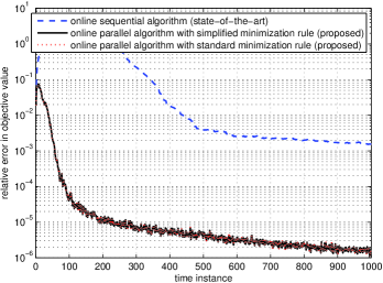
Figure 1: Convergence behavior in terms of objective function value.

In this section, the desirable features of the proposed algorithm are illustrated numerically.

We first test the convergence behavior of Algorithm 1 with the online sequential algorithm proposed in [14]. In this example, the parameters are selected as follows:

• $N=1$, so the subscript $n$ is omitted.

• the dimension of $\mathbf{x}^{\star}$: $K=100$;

• the density of $\mathbf{x}^{\star}$: 0.1;

• Both $\mathbf{g}$ and $v$ are generated by i.i.d. standard normal distributions: $\mathbf{g}\in\mathcal{CN}(\mathbf{0},\mathbf{I})$ and $v\in\mathcal{CN}(0,0.2)$;

• The sparsity regularization gain $\mu^{(t)}=\sqrt{K}/t=10/t$;

• Unless otherwise stated, the simulations results are averaged over 100 realizations.

We plot in Figure 1 the relative error in objective value $(L^{(t)}(\mathbf{x}^{(t)})-L^{(t)}(\mathbf{x}_{\textrm{lasso}}^{(t)}))/L^{(t)}(\mathbf{x}_{\textrm{lasso}}^{(t)})$ versus the time instance $t$, where 1) $\mathbf{x}_{\textrm{lasso}}^{(t)}$ is defined in (6) and calculated by MOSEK [33]; 2) $\mathbf{x}^{(t)}$ is returned by Algorithm 1 in the proposed online parallel algorithm; 3) $\mathbf{x}^{(t)}$ is returned by [14, Algorithm 1] in online sequential algorithm; and 4) $\mathbf{x}^{(1)}=\mathbf{0}$ for both parallel and sequential algorithms. Note that $L^{(t)}(\mathbf{x}_{\textrm{lasso}}^{(t)})$ is by definition the lower bound of $L^{(t)}(\mathbf{x})$ and $L^{(t)}(\mathbf{x}^{(t)})-L^{(t)}(\mathbf{x}_{\textrm{lasso}}^{(t)})\geq 0$ for all $t$. From Figure 1 it is clear that the proposed algorithm (black curve) converges to a precision of $10^{-2}$ in less than 200 instances while the sequential algorithm (blue curve) needs more than 800 instances. The improvement in convergence speed is thus notable. If the precision is set as $10^{-4}$, the sequential algorithm does not even converge in a reasonable number of instances. Therefore, the proposed online parallel algorithm outperforms in both convergence speed and solution quality.

We also evaluate in Figure 1 the performance loss incurred by the simplified minimization rule (21) (indicated by the black curve) compared with the standard minimization rule (18) (indicated by the red curve). It is easy to see from Figure 1 that these two curves almost coincide with each other, so the extent to which the simplified minimization rule decreases the objective function is nearly as same as standard minimization rule and the performance loss is negligible.

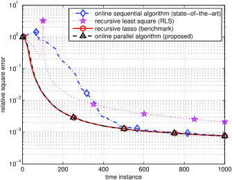
Figure 2: Convergence behavior in terms of relative square error.

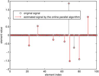
Figure 3: Comparison of original signal and estimated signal.

Then we consider in Figure 3 the relative square error $\left\|\mathbf{x}^{(t)}-\mathbf{x}^{\star}\right\|_{2}^{2}/\left\|\mathbf{x}^{\star}\right\|_{2}^{2}$ versus the time instance $t$, where the benchmark is $\bigl{\|}\mathbf{x}_{\textrm{lasso}}^{(t)}-\mathbf{x}^{\star}\bigr{\|}_{2}^{2}/\left\|\mathbf{x}^{\star}\right\|_{2}^{2}$, i.e., the recursive Lasso (6). To compare the estimation approaches with and without sparsity regularization, RLS in (6) is also implemented, where a $\ell_{2}$ regularization term $(10^{-4}/t)\cdot\left\|\mathbf{x}\right\|_{2}^{2}$ is included into (6) when $\mathbf{G}^{(t)}$ is singular. We see that the relative square error of the proposed online parallel algorithm quickly reaches the benchmark (recursive lasso) in about 100 instances, while the sequential algorithm needs about 800 instances. The improvement in convergence speed is consolidated again. Another notable feature is that, the relative square error of the proposed algorithm is always decreasing, even in beginning instances, while the relative square error of the sequential algorithm is not: in the first 100 instances, the relative square error is actually increasing. Recall the signal dimension ($K=100$), we infer that the relative square error starts to decrease only after each element has been updated once. What is more, estimation with sparsity regularization performs better than the classic RLS approach because they exploit the a prior sparsity of the to-be-estimated signal $\mathbf{x}^{\star}$. The precision of the estimated signal by the proposed online parallel algorithm (after 1000 time instances) is also shown element-wise in Figure 3, from which we observe that both the zeros and the nonzero elements of the original signal $\mathbf{x}^{\star}$ are estimated accurately.

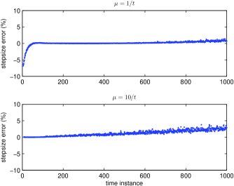
Figure 4: Stepsize error of the simplified minimization rule.

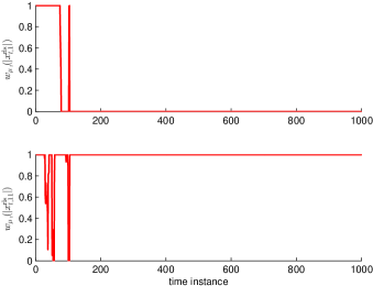
Figure 5: Weight factor in time- and norm-weighted sparsity regularization.

We now compare the proposed simplified minimization rule (cf. (21)-(16)), coined as stepsize_simplified, with the standard minimization rule (cf. (18)), coined as stepsize_optimal, in terms of the stepsize error defined as follows:

$$\frac{\textrm{stepsize\_simplified-stepsize\_optimal}}{\textrm{stepsize\_optimal}}\times 100\%.$$

In addition to the above parameter where $\mu^{(t)}=10/t$ (in the lower subplot), we also simulate the case when $\mu^{(t)}=1/t$ (in the upper subplot). We see from Figure 5 that the stepsize error is reasonably small, namely, mainly in the interval [-5%,5%], while only a few of beginning instances are outside this region, so the simplified minimization rule achieves a good trade-off between performance and complexity. Comparing the two subplots, we find that, as expected, the stepsize error depends on the value of $\mu$. We can also infer that the simplified minimization rule tends to overestimate the optimal stepsize.

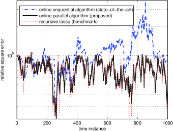
Figure 6: Relative square error for recursive estimation of time-varying signals

In Figure 5 we simulate the weight factor $\mathcal{W}_{\mu^{(t)}}(|x_{\textrm{rls},k}^{(t)}|)$ versus the time instance $t$ in time- and norm-weighted sparsity regularization, where $k=1$ in the upper plot and $k=11$ in the lower plot. The parameters are as same as the above examples, except that $\mu^{(t)}=1/t^{0.4}$ and $\mathbf{x}^{\star}$ are generated such that the first $0.1\times K$ elements (where 0.1 is the density of $\mathbf{x}^{\star}$) are nonzero while all other elements are zero. The weight factors of other elements are omitted because they exhibit similar behavior as the ones plotted in Figure 5. As analyzed, $\mathcal{W}_{\mu^{(t)}}(|w_{\textrm{rls},1}^{(t)}|)$, the weight factor of the first element, where $x_{1}^{\star}\neq 0$, quickly converges to 0, while $\mathcal{W}_{\mu^{(t)}}(|w_{\textrm{rls},11}^{(t)}|)$, the weight factor of the eleventh element, where $x_{1}^{\star}=0$ , quickly converges to $1$, making the overall weight factor monotonically decreasing, cf. (29). Therefore the proposed algorithm can readily be applied to the recursive estimation of sparse signals with time- and norm-weighted regularization.

When the signal to be estimated is time-varying, the theoretical analysis of the proposed algorithm is not valid anymore, but we can test numerically how the proposed algorithm performs compared with the online sequential algorithm. The time-varying unknown signal is denoted as $\mathbf{x}_{t}^{\star}$, and it is changing according to the following law:

$$x_{t+1,k}^{\star}=\alpha x_{t,k}^{\star}+w_{t,k},$$

where $w_{t,k}\sim\mathcal{CN}(0,1-\alpha^{2})$ for any $k$ such that $x_{t,k}^{\star}\neq 0$, with $\alpha=0.99$ and $\beta=0.9$. In Figure 6, the relative square error $\left\|\mathbf{x}_{t}-\mathbf{x}_{t}^{\star}\right\|_{2}^{2}/\left\|\mathbf{x}_{t}^{\star}\right\|_{2}^{2}$ is plotted versus the time instance. Despite the lack of theoretical consolidation, we observe the online parallel algorithm is almost as same as the pseudo-online algorithm, so the inexact optimization is not an impeding factor for the estimation accuracy. This also consolidates the superiority of the proposed algorithm over [1] where a distributed iterative algorithm is employed to solve (30) exactly, which inevitably incurs a large delay and extensive signaling.

VI Concluding Remarks

In this paper, we have considered the recursive estimation of sparse signals and proposed an online parallel algorithm with provable convergence. The algorithm is based on inexact optimization with an increasing accuracy and parallel update of all elements at each time instance, where both the update direction and the stepsize can be calculated in closed-form expressions. The proposed simplified minimization stepsize rule is well motivated and easily implementable, achieving a good trade-off between complexity and convergence speed, and avoiding the common drawbacks of the decreasing stepsizes used in literature. Simulation results consolidate the notable improvement in convergence speed over state-of-the-art techniques, and they also show that the loss in convergence speed compared with the full version (where the lasso problem is solved exactly at each time instance) is negligible. We have also considered numerically the recursive estimation of time-varying signals where theoretical convergence do not necessarily hold, and the proposed algorithm works better than state-of-the-art algorithms.

Appendix A Proof of Theorem 4

Proof:

It is easy to see that $L^{(t)}$ can be divided into a smooth part $f^{(t)}(\mathbf{x})$ and a nonsmooth part $h^{(t)}(\mathbf{x})$:

$$f^{(t)}(\mathbf{x}) \triangleq\frac{1}{2}\mathbf{x}^{T}\mathbf{G}^{(t)}\mathbf{x}-(\mathbf{b}^{(t)})^{T}\mathbf{x},$$ (31a)

$$h^{(t)}(\mathbf{x}) \triangleq\mu^{(t)}\left\|\mathbf{x}\right\|_{1}.$$ (31b)

We also use $f_{k}^{(t)}(x;\mathbf{x}^{(t)})$ to denote the smooth part of the objective function in (11):

$$f_{k}^{(t)}(x;\mathbf{x}^{(t)})\triangleq\frac{1}{2}G_{kk}^{(t)}x^{2}-r_{k}^{(t)}\cdot x+\frac{1}{2}c_{k}^{(t)}(x-x_{k}^{(t)})^{2}.$$ (32)

Functions $f_{k}^{(t)}(x;\mathbf{x}^{(t)})$ and $f^{(t)}(\mathbf{x})$ are related according to the following equation:

$$f_{k}^{(t)}(x_{k};\mathbf{x}^{(t)})=f^{(t)}(x_{k},\mathbf{x}_{-k}^{(t)})+\frac{1}{2}c^{(t)}(x_{k}-x_{k}^{(t)})^{2},$$ (33)

from which it is easy to infer that $\nabla f_{k}^{(t)}(x_{k}^{(t)};\mathbf{x}^{(t)})=\nabla_{k}f^{(t)}(\mathbf{x}^{(t)})$. Then from the first-order optimality condition, $h^{(t)}(x_{k})$ has a subgradient $\xi_{k}^{(t)}\in\partial h^{(t)}(\hat{x}_{k}^{(t)})$ at $x_{k}=\hat{x}_{k}^{(t)}$ such that for any $x_{k}$:

$$(x_{k}-\hat{x}_{k}^{(t)})(\nabla f_{k}^{(t)}(\hat{x}_{k}^{(t)};\mathbf{x}^{(t)})+\xi_{k}^{(t)})\geq 0,\,\forall k.$$ (34)

Now consider the following equation:

$$\begin{array}[]{l}L^{(t)}(\mathbf{x}^{(t+1)})-L^{(t-1)}(\mathbf{x}^{(t)})=\vskip 3.0pt plus 1.0pt minus 1.0pt\\ \qquad L^{(t)}(\mathbf{x}^{(t+1)})-L^{(t)}(\mathbf{x}^{(t)})+L^{(t)}(\mathbf{x}^{(t)})-L^{(t-1)}(\mathbf{x}^{(t)}).\end{array}$$ (35)

The rest of the proof consists of three parts. Firstly we prove that there exists a constant $\eta>0$ such that $L^{(t)}(\mathbf{x}^{(t+1)})-L^{(t)}(\mathbf{x}^{(t)})\leq-\eta\left\|\hat{\mathbf{x}}^{(t)}-\mathbf{x}^{(t)}\right\|_{2}^{2}$. Then we show that the sequence $\left\{L^{(t)}(\mathbf{x}^{(t+1)})\right\}_{t}$ converges. Finally we prove that any limit point of the sequence $\left\{\mathbf{x}^{(t)}\right\}_{t}$ is a solution of (2).

Part 1) Since $c_{\min}^{(t)}\geq c>0$ for all $t$ ($c_{\textrm{min}}^{(t)}$ is defined in Proposition 2) from Assumption (A5), it is easy to see from (14) that the following is true:

$$L^{(t)}(\mathbf{x}^{(t)}+\gamma(\hat{\mathbf{x}}^{(t)}-\mathbf{x}^{(t)}))-L^{(t)}(\mathbf{x}^{(t)})$$

$$\leq\; -\gamma\Bigl{(}c-\frac{1}{2}\lambda_{\max}(\mathbf{G}^{(t)})\gamma\Bigr{)}\bigl{\|}\hat{\mathbf{x}}^{(t)}-\mathbf{x}^{(t)}\bigr{\|}_{2}^{2},\,0\leq\gamma\leq 1.$$

Since $\lambda_{\max}(\bullet)$ is a continuous function [34] and $\mathbf{G}^{(t)}$ converges to a positive definite matrix by Assumption (A1), there exists a $\bar{\lambda}<+\infty$ such that $\bar{\lambda}\geq\lambda_{\max}(\mathbf{G}^{(t)})$ for all $t$. We thus conclude from the preceding inequality that for all $0\leq\lambda\leq 1$:

$$L^{(t)}(\mathbf{x}^{(t)}+\gamma(\hat{\mathbf{x}}^{(t)}-\mathbf{x}^{(t)}))-L^{(t)}(\mathbf{x}^{(t)})$$

$$\leq -\gamma\left(c-\frac{1}{2}\bar{\lambda}\gamma\right)\bigl{\|}\hat{\mathbf{x}}^{(t)}-\mathbf{x}^{(t)}\bigr{\|}_{2}^{2}.$$ (36)

It follows from (20), (21) and (36) that

$$L^{(t)}(\tilde{\mathbf{x}}^{(t+1)})$$

$$\leq\; f^{(t)}(\mathbf{x}^{(t)}+\gamma^{(t)}(\hat{\mathbf{x}}^{(t)}-\mathbf{x}^{(t)}))$$

$$+(1-\gamma^{(t)})h^{(t)}(\mathbf{x}^{(t)})+\gamma^{(t)}h^{(t)}(\hat{\mathbf{x}}^{(t)})$$ (37)

$$\leq\; f^{(t)}(\mathbf{x}^{(t)}+\gamma(\hat{\mathbf{x}}^{(t)}-\mathbf{x}^{(t)}))$$

$$+(1-\gamma)h^{(t)}(\mathbf{x}^{(t)})+\gamma h^{(t)}(\hat{\mathbf{x}}^{(t)})$$ (38)

$$\leq\; L^{(t)}(\mathbf{x}^{(t)})-\gamma(c-\frac{1}{2}\bar{\lambda}\gamma)\bigl{\|}\hat{\mathbf{x}}^{(t)}-\mathbf{x}^{(t)}\bigr{\|}_{2}^{2}.$$ (39)

Since the inequalities in (39) are true for any $0\leq\gamma\leq 1$, we set $\gamma=\min(c/\bar{\lambda},1)$. Then it is possible to show that there is a constant $\eta>0$ such that

$$L^{(t)}(\mathbf{x}^{(t+1)})-L^{(t)}(\mathbf{x}^{(t)}) \leq L^{(t)}(\tilde{\mathbf{x}}^{(t+1)})-L^{(t)}(\mathbf{x}^{(t)})$$

$$\leq-\eta\bigl{\|}\hat{\mathbf{x}}^{(t)}-\mathbf{x}^{(t)}\bigr{\|}_{2}^{2}.$$ (40)

Besides, because of Step 3 in Algorithm 1, $\mathbf{x}^{(t+1)}$ is in the following lower level set of $L^{(t)}(\mathbf{x})$:

$$\mathcal{L}_{\leq 0}^{(t)}\triangleq\{\mathbf{x}:L^{(t)}(\mathbf{x})\leq 0\}.$$ (41)

Because $\left\|\mathbf{x}\right\|_{1}\geq 0$ for any $\mathbf{x}$, (41) is a subset of

$$\left\{\mathbf{x}:\frac{1}{2}\mathbf{x}^{T}\mathbf{G}^{(t)}\mathbf{x}-(\mathbf{b}^{(t)})^{T}\mathbf{x}\leq 0\right\},$$

which is a subset of

$$\bar{\mathcal{L}}_{\leq 0}^{(t)}\triangleq\left\{\mathbf{x}:\frac{1}{2}\lambda_{\max}(\mathbf{G}^{(t)})\left\|\mathbf{x}\right\|_{2}^{2}-(\mathbf{b}^{(t)})^{T}\mathbf{x}\leq 0\right\}.$$ (42)

Since $\mathbf{G}^{(t)}$ and $\mathbf{b}^{(t)}$ converges and $\lim_{t\rightarrow\infty}\mathbf{G}^{(t)}\succ\mathbf{0}$, there exists a bounded set, denoted as $\mathcal{L}_{\leq 0}$, such that $\mathcal{L}_{\leq 0}^{(t)}\subseteq\bar{\mathcal{L}}_{\leq 0}^{(t)}\subseteq\mathcal{L}_{\leq 0}$ for all $t$; thus the sequence $\{\mathbf{x}^{(t)}\}$ is bounded and we denote its upper bound as $\bar{\mathbf{x}}$.

Part 2) Combining (35) and (40), we have the following:

$$L^{(t+1)}(\mathbf{x}^{(t+2)})\negmedspace-\negmedspace L^{(t)}(\mathbf{x}^{(t+1)})$$

$$\leq\, L^{(t+1)}(\mathbf{x}^{(t+1)})\negmedspace-\negmedspace L^{(t)}(\mathbf{x}^{(t+1)})$$

$$=\, f^{(t+1)}(\mathbf{x}^{(t+1)})\negmedspace-\negmedspace f^{(t)}(\mathbf{x}^{(t+1)})\negmedspace+\negmedspace h^{(t+1)}(\mathbf{x}^{(t+1)})\negmedspace-\negmedspace h^{(t)}(\mathbf{x}^{(t+1)})$$

$$\leq\, f^{(t+1)}(\mathbf{x}^{(t+1)})\negmedspace-\negmedspace f^{(t)}(\mathbf{x}^{(t+1)}),$$ (43)

where the last inequality comes from the decreasing property of $\mu^{(t)}$ by Assumption (A6). Recalling the definition of $f^{(t)}(\mathbf{x})$ in (31), it is easy to see that

$$(t+1)(f^{(t+1)}(\mathbf{x}^{(t+1)})-f^{(t)}(\mathbf{x}^{(t+1)}))$$

$$=l^{(t+1)}(\mathbf{x}^{(t+1)}) -\frac{1}{t}\sum_{\tau=1}^{t}l^{(\tau)}(\mathbf{x}^{(t+1)}),$$

where

$$l^{(t)}(\mathbf{x})\triangleq\sum_{n=1}^{N}(y_{n}^{(t)}-(\mathbf{g}_{n}^{(t)})^{T}\mathbf{x})^{2}.$$

Taking the expectation of the preceding equation with respect to $\{y_{n}^{(t+1)},\mathbf{g}_{n}^{(t+1)}\}_{n=1}^{N}$, conditioned on the natural history up to time $t+1$, denoted as $\mathcal{F}^{(t+1)}$:

$$\begin{array}[]{l}\mathcal{F}^{(t+1)}=\vskip 3.0pt plus 1.0pt minus 1.0pt\\ \quad\left\{\mathbf{x}^{(0)},\ldots,\mathbf{x}^{(t+1)},\bigl{\{}\mathbf{g}_{n}^{(0)},\ldots,\mathbf{g}_{n}^{(t)}\bigr{\}}_{n},\bigl{\{}y_{n}^{(0)},\ldots,y_{n}^{(t)}\bigr{\}}_{n}\right\},\end{array}$$

we have

$$\mathbb{E}\left[(t+1)(f^{(t+1)}(\mathbf{x}^{(t+1)})-f^{(t)}(\mathbf{x}^{(t+1)}))|\mathcal{F}^{(t+1)}\right]$$

$$=\; \mathbb{E}\left[l^{(t+1)}(\mathbf{x}^{(t+1)})|\mathcal{F}^{(t+1)}\right]-\frac{1}{t}\sum_{\tau=1}^{t}\mathbb{E}\left[l^{(\tau)}(\mathbf{x}^{(t+1)})|\mathcal{F}^{(t+1)}\right]$$

$$=\; \mathbb{E}\left[l^{(t+1)}(\mathbf{x}^{(t+1)})|\mathcal{F}^{(t+1)}\right]-\frac{1}{t}\sum_{\tau=1}^{t}l^{(\tau)}(\mathbf{x}^{(t+1)}),$$ (44)

where the second equality comes from the observation that $l^{(\tau)}(\mathbf{x}^{(t+1)})$ is deterministic as long as $\mathcal{F}^{(t+1)}$ is given. This together with (43) indicates that

$$\mathbb{E}\left[L^{(t+1)}(\mathbf{x}^{(t+2)})-L^{(t)}(\mathbf{x}^{(t+1)})|\mathcal{F}^{(t+1)}\right]$$

$$\leq\; \mathbb{E}\left[f^{(t+1)}(\mathbf{x}^{(t+1)})-f^{(t)}(\mathbf{x}^{(t+1)})|\mathcal{F}^{(t+1)}\right]$$

$$\leq\; \frac{1}{t+1}\left(\mathbb{E}\left[l^{(t+1)}(\mathbf{x}^{(t+1)})|\mathcal{F}^{(t+1)}\right]-\frac{1}{t}\sum_{\tau=1}^{t}l^{(\tau)}(\mathbf{x}^{(t+1)})\right)$$

$$\leq\; \frac{1}{t+1}\left|\mathbb{E}\left[l^{(t+1)}(\mathbf{x}^{(t+1)})|\mathcal{F}^{(t+1)}\right]-\frac{1}{t}\sum_{\tau=1}^{t}l^{(\tau)}(\mathbf{x}^{(t+1)})\right|,$$

and

$$\left[\mathbb{E}\left[L^{(t+1)}(\mathbf{x}^{(t+2)})-L^{(t)}(\mathbf{x}^{(t+1)})|\mathcal{F}^{(t+1)}\right]\right]_{0}$$

$$\leq\; \frac{1}{t+1}\left|\mathbb{E}\left[l^{(t+1)}(\mathbf{x}^{(t+1)})|\mathcal{F}^{(t+1)}\right]-\frac{1}{t}\sum_{\tau=1}^{t}l^{(\tau)}(\mathbf{x}^{(t+1)})\right|$$

$$\leq\; \frac{1}{t+1}\sup_{\mathbf{x}\in\mathcal{X}}\left|\mathbb{E}\left[l^{(t+1)}(\mathbf{x})|\mathcal{F}^{(t+1)}\right]-\frac{1}{t}\sum_{\tau=1}^{t}l^{(\tau)}(\mathbf{x})\right|,$$ (45)

where $[x]_{0}=\max(x,0)$, and $\mathcal{X}$ in (45) with $\mathcal{X}\triangleq\{\mathbf{x}^{(1)},\mathbf{x}^{(2)},\ldots,\}$ is the complete path of $\mathbf{x}$.

Now we derive an upper bound on the expected value of the right hand side of (45):

$$\mathbb{E}\left[\sup_{\mathbf{x}\in\mathcal{X}}\left|\mathbb{E}\left[l^{(t+1)}(\mathbf{x})|\mathcal{F}^{(t+1)}\right]-\frac{1}{t}\sum_{\tau=1}^{t}l^{(\tau)}(\mathbf{x})\right|\right]$$

$$=\; \mathbb{E}\left[\sup_{\mathbf{x}\in\mathcal{X}}\bigl{|}\breve{y}^{(t)}-(\mathbf{r}_{2}^{(t)})^{T}\mathbf{x}+\mathbf{x}^{T}\mathbf{R}_{3}^{(t)}\mathbf{x}\bigr{|}\right]$$

$$\leq\; \mathbb{E}\left[\sup_{\mathbf{x}\in\mathcal{X}}\bigl{|}\breve{y}^{(t)}\bigr{|}+\sup_{\mathbf{x}\in\mathcal{X}}\bigl{|}(\breve{\mathbf{b}}^{(t)})^{T}\mathbf{x}\bigr{|}+\sup_{\mathbf{x}\in\mathcal{X}}\bigl{|}\mathbf{x}^{T}\breve{\mathbf{G}}^{(t)}\mathbf{x}\bigr{|}\right]$$

$$=\; \mathbb{E}\left[\sup_{\mathbf{x}\in\mathcal{X}}\bigl{|}\breve{y}^{(t)}\bigr{|}\right]+\mathbb{E}\left[\sup_{\mathbf{x}\in\mathcal{X}}\bigl{|}(\breve{\mathbf{b}}^{(t)})^{T}\mathbf{x}\bigr{|}\right]+\mathbb{E}\left[\sup_{\mathbf{x}\in\mathcal{X}}\bigl{|}\mathbf{x}^{T}\breve{\mathbf{G}}^{(t)}\mathbf{x}\bigr{|}\right],$$ (46)

where

$$\breve{y}^{(t)} \triangleq\frac{1}{t}\sum_{\tau=1}^{t}\sum_{n=1}^{N}\left(\mathbb{E}_{y_{n}}\left[y_{n}^{2}\right]-(y_{n}^{(\tau)})^{2}\right),$$

$$\breve{\mathbf{b}}^{(t)} \triangleq\frac{1}{t}\sum_{\tau=1}^{t}\sum_{n=1}^{N}2\left(\mathbb{E}_{\{y_{n},\mathbf{g}_{n}\}}\left[y_{n}\mathbf{g}_{n}\right]-y_{n}^{(\tau)}\mathbf{g}_{n}^{(\tau)}\right),$$

$$\breve{\mathbf{G}}^{(t)} \triangleq\frac{1}{t}\sum_{\tau=1}^{t}\sum_{n=1}^{N}\left(\mathbb{E}_{\mathbf{g}_{n}}\left[\mathbf{g}_{n}\mathbf{g}_{n}\right]-\mathbf{g}_{n}^{(t)}\mathbf{g}_{n}^{(\tau)T}\right).$$

Then we bound each term in (46) individually. For the first term, since $\breve{y}^{(t)}$ is independent of $\mathbf{x}^{(t)}$,

$$\mathbb{E}\left[\sup_{\mathbf{x}\in\mathcal{X}}\bigl{|}\breve{y}^{(t)}\bigr{|}\right]=\mathbb{E}\left[\bigl{|}\breve{y}^{(t)}\bigr{|}\right] =\mathbb{E}\left[\sqrt{(\breve{y}^{(t)})^{2}}\right]$$

$$\leq\sqrt{\mathbb{E}\left[(\breve{y}^{(t)})^{2}\right]}\leq\sqrt{\frac{\sigma_{1}^{2}}{t}}$$ (47)

for some $\sigma_{1}<\infty$, where the second equality comes from Jensen’s inequality. Because of Assumptions (A1), (A2) and (A4), $\breve{y}^{(t)}$ has bounded moments and the existence of $\sigma_{1}$ is then justified by the central limit theorem [35].

For the second term of (46), we have

$$\mathbb{E}\left[\sup_{\mathbf{x}}\bigl{|}(\breve{\mathbf{b}}^{(t)})^{T}\mathbf{x}\bigr{|}\right] \negmedspace\leq\negthinspace\mathbb{E}\left[\sup_{\mathbf{x}}(\bigl{|}\breve{\mathbf{b}}^{(t)}\bigr{|})^{T}\left|\mathbf{x}\right|\right]\negmedspace\leq\negmedspace\left(\mathbb{E}\left[\bigl{|}\breve{\mathbf{b}}^{(t)}\bigr{|}\right]\right)^{\negmedspace T}\negmedspace\left|\bar{\mathbf{x}}\right|.$$

Similar to the line of analysis of (47), there exists a $\sigma_{2}<\infty$ such that

$$\mathbb{E}\left[\sup_{\mathbf{x}}\bigl{|}(\breve{\mathbf{b}}^{(t)})^{T}\mathbf{x}\bigr{|}\right]\leq\left(\mathbb{E}\left[\bigl{|}\breve{\mathbf{b}}^{(t)}\bigr{|}\right]\right)^{T}\left|\bar{\mathbf{x}}\right|\leq\sqrt{\frac{\sigma_{2}^{2}}{t}}.$$ (48)

For the third term of (46), we have

$$\mathbb{E}\left[\sup_{\mathbf{x}\in\mathcal{X}}\bigl{|}\mathbf{x}^{T}\breve{\mathbf{G}}^{(t)}\mathbf{x}\bigr{|}\right]$$

$$=\; \mathbb{E}\left[\max_{1\leq k\leq K}\bigl{|}\lambda_{k}(\breve{\mathbf{G}}^{(t)})\bigr{|}\cdot\left\|\bar{\mathbf{x}}\right\|_{2}^{2}\right]$$

$$=\; \left\|\bar{\mathbf{x}}\right\|_{2}^{2}\cdot\mathbb{E}\left[\sqrt{\max\{\lambda_{\max}^{2}(\breve{\mathbf{G}}^{(t)}),\lambda_{\min}^{2}(\breve{\mathbf{G}}^{(t)})\}}\right]$$

$$\leq\; \left\|\bar{\mathbf{x}}\right\|_{2}^{2}\cdot\sqrt{\mathbb{E}\left[\max\{\lambda_{\max}^{2}(\breve{\mathbf{G}}^{(t)}),\lambda_{\min}^{2}(\breve{\mathbf{G}}^{(t)})\}\right]}$$

$$\leq\; \left\|\bar{\mathbf{x}}\right\|_{2}^{2}\cdot\sqrt{\mathbb{E}\left[\sum_{k=1}^{K}\lambda_{k}^{2}(\breve{\mathbf{G}}^{(t)})\right]}$$

$$=\; \left\|\bar{\mathbf{x}}\right\|_{2}^{2}\cdot\sqrt{\mathbb{E}\left[\textrm{tr}\left(\breve{\mathbf{G}}^{(t)}(\breve{\mathbf{G}}^{(t)})^{T}\right)\right]}\leq\sqrt{\frac{\sigma_{3}^{2}}{t}}$$ (49)

for some $\sigma_{3}<\infty$, where the first equality comes from the observation that $\mathbf{x}$ should align with the eigenvector associated with the eigenvalue with largest absolute value. Then combing (47)-(49), we can claim that there exists $\sigma\triangleq\sqrt{\sigma_{1}^{2}}+\sqrt{\sigma_{2}^{2}}+\sqrt{\sigma_{3}^{2}}>0$ such that

$$\mathbb{E}\left[\sup_{\mathbf{x}\in\mathcal{X}}\left|\mathbb{E}\left[l^{(t+1)}(\mathbf{x})|\mathcal{F}^{(t+1)}\right]-\frac{1}{t}\sum_{\tau=1}^{t}l^{(\tau)}(\mathbf{x})\right|\right]\leq\frac{\sigma}{\sqrt{t}}.$$

In view of (45), we have

$$\mathbb{E}\left[\left[\mathbb{E}\left[L^{(t+1)}(\mathbf{x}^{(t+2)})-L^{(t)}(\mathbf{x}^{(t+1)})|\mathcal{F}^{(t+1)}\right]\right]_{0}\right]\leq\frac{\sigma}{t^{3/2}}.$$ (50)

Summing (50) over $t$, we obtain

$$\sum_{t=1}^{\infty}\mathbb{E}\left[\left[\mathbb{E}\left[L^{(t+1)}(\mathbf{x}^{(t+2)})-L^{(t)}(\mathbf{x}^{(t+1)})|\mathcal{F}^{(t+1)}\right]\right]_{0}\right]<\infty.$$

Then it follows from the quasi-martingale convergence theorem (cf. [30, Th. 6]) that $\left\{L^{(t)}(\mathbf{x}^{(t+1)})\right\}$ converges almost surely.

Part 3) Combining (35) and (40), we have

$$L^{(t)}(\mathbf{x}^{(t+1)})-L^{(t-1)}(\mathbf{x}^{(t)}) \leq$$

$$-\eta\bigl{\|}\hat{\mathbf{x}}^{(t)}-\mathbf{x}^{(t)}\bigr{\|}_{2}^{2}+ L^{(t)}(\mathbf{x}^{(t)})-L^{(t-1)}(\mathbf{x}^{(t)}).$$ (51)

Besides, it follows from the convergence of $\left\{L^{(t)}(\mathbf{x}^{(t+1)})\right\}_{t}$

$$\lim_{t\rightarrow\infty}L^{(t)}(\mathbf{x}^{(t+1)})-L^{(t-1)}(\mathbf{x}^{(t)})=0,$$

and the strong law of large numbers that

$$\lim_{t\rightarrow\infty}L^{(t)}(\mathbf{x}^{(t)})-L^{(t-1)}(\mathbf{x}^{(t)})=0.$$

Taking the limit inferior of both sides of (51), we have

$$\begin{split}0&=\underset{t\rightarrow\infty}{\lim\inf}\left\{L^{(t)}(\mathbf{x}^{(t+1)})-L^{(t-1)}(\mathbf{x}^{(t)})\right\}\\ &\leq\underset{t\rightarrow\infty}{\lim\inf}\left\{-\eta\bigl{\|}\hat{\mathbf{x}}^{(t)}-\mathbf{x}^{(t)}\bigr{\|}_{2}^{2}+L^{(t)}(\mathbf{x}^{(t)})-L^{(t-1)}(\mathbf{x}^{(t)})\right\}\\ &\leq\underset{t\rightarrow\infty}{\lim\inf}\left\{-\eta\bigl{\|}\hat{\mathbf{x}}^{(t)}-\mathbf{x}^{(t)}\bigr{\|}_{2}^{2}\right\}\\ &\qquad\quad+\underset{t\rightarrow\infty}{\lim\sup}\left\{L^{(t)}(\mathbf{x}^{(t)})-L^{(t-1)}(\mathbf{x}^{(t)})\right\}\\ &=-\eta\cdot\underset{t\rightarrow\infty}{\lim\sup}\bigl{\|}\hat{\mathbf{x}}^{(t)}-\mathbf{x}^{(t)}\bigr{\|}_{2}^{2}\leq 0,\end{split}$$

so we can infer that $\lim\sup_{t\rightarrow\infty}\bigl{\|}\hat{\mathbf{x}}^{(t)}-\mathbf{x}^{(t)}\bigr{\|}_{2}=0$. Since $0\leq\lim\inf_{t\rightarrow\infty}\bigl{\|}\hat{\mathbf{x}}^{(t)}-\mathbf{x}^{(t)}\bigr{\|}_{2}\leq\lim\sup_{t\rightarrow\infty}\bigl{\|}\hat{\mathbf{x}}^{(t)}-\mathbf{x}^{(t)}\bigr{\|}_{2}=0$, we can infer that $\lim\inf_{t\rightarrow\infty}\bigl{\|}\hat{\mathbf{x}}^{(t)}-\mathbf{x}^{(t)}\bigr{\|}=0$ and thus $\lim_{t\rightarrow\infty}\bigl{\|}\hat{\mathbf{x}}^{(t)}-\mathbf{x}^{(t)}\bigr{\|}=0$.

Consider any limit point of the sequence $\left\{\mathbf{x}^{(t)}\right\}_{t}$, denoted as $\mathbf{x}^{(\infty)}$. Since $\hat{\mathbf{x}}$ is a continuous function of $\mathbf{x}$ in view of (11) and $\lim_{t\rightarrow\infty}\left\|\hat{\mathbf{x}}^{(t)}-\mathbf{x}^{(t)}\right\|_{2}=0$, it must be $\lim_{t\rightarrow\infty}\hat{\mathbf{x}}^{(t)}=\hat{\mathbf{x}}^{(\infty)}=\mathbf{x}^{(\infty)}$, and the minimum principle in (34) can be simplified as

$$(x_{k}-x_{k}^{(\infty)})(\nabla_{k}f^{(\infty)}(\mathbf{x}^{(\infty)})+\xi_{k}^{(\infty)})\geq 0,\;\forall x_{k},$$

whose summation over $k=1,\ldots,K$ leads to

$$(\mathbf{x}-\mathbf{x}^{(\infty)})^{T}(\nabla f^{(\infty)}(\mathbf{x}^{(\infty)})+\boldsymbol{\xi}^{(\infty)})\geq 0,\quad\forall\mathbf{x}.$$

Therefore $\mathbf{x}^{(\infty)}$ minimizes $L^{(\infty)}(\mathbf{x})$ and $\mathbf{x}^{(\infty)}=\mathbf{x}^{\star}$ almost surely by Lemma 1. Since $\mathbf{x}^{\star}$ is unique in view of Assumptions (A1)-(A3), the whole sequence $\{\mathbf{x}^{(t)}\}$ has a unique limit point and it thus converges to $\mathbf{x}^{\star}$. The proof is thus completed. ∎

References

• [1] S. Barbarossa, S. Sardellitti, and P. Di Lorenzo, “Distributed detection and estimation in wireless sensor networks,” in Academic Press Library in Signal Processing, R. Chellappa and S. Theodoridis, Eds., 2014, vol. 2, pp. 329–408.
• [2] S. Haykin, “Cognitive radio: brain-empowered wireless communications,” IEEE Journal on Selected Areas in Communications, vol. 23, no. 2, pp. 201–220, Feb. 2005.
• [3] J. Mitola and G. Maguire, “Cognitive radio: making software radios more personal,” IEEE Personal Communications, vol. 6, no. 4, pp. 13–18, 1999.
• [4] R. Zhang, Y.-C. Liang, and S. Cui, “Dynamic Resource Allocation in Cognitive Radio Networks,” IEEE Signal Processing Magazine, vol. 27, no. 3, pp. 102–114, May 2010.
• [5] Y. Yang, G. Scutari, P. Song, and D. P. Palomar, “Robust MIMO Cognitive Radio Systems Under Interference Temperature Constraints,” IEEE Journal on Selected Areas in Communications, vol. 31, no. 11, pp. 2465–2482, Nov. 2013.
• [6] S. Haykin, D. Thomson, and J. Reed, “Spectrum Sensing for Cognitive Radio,” Proceedings of the IEEE, vol. 97, no. 5, pp. 849–877, May 2009.
• [7] S.-J. Kim, E. Dall’Anese, and G. B. Giannakis, “Cooperative Spectrum Sensing for Cognitive Radios Using Kriged Kalman Filtering,” IEEE Journal of Selected Topics in Signal Processing, vol. 5, no. 1, pp. 24–36, Feb. 2011.
• [8] F. Zeng, C. Li, and Z. Tian, “Distributed Compressive Spectrum Sensing in Cooperative Multihop Cognitive Networks,” IEEE Journal of Selected Topics in Signal Processing, vol. 5, no. 1, pp. 37–48, Feb. 2011.
• [9] O. Mehanna and N. D. Sidiropoulos, “Frugal Sensing: Wideband Power Spectrum Sensing From Few Bits,” IEEE Transactions on Signal Processing, vol. 61, no. 10, pp. 2693–2703, May 2013.
• [10] S. M. Kay, Fundamentals of Statistical Signal Processing, Volume I: Estimation Theory.   Prentice Hall, 1993.
• [11] A. Sayed, Adaptive filters.   Hoboken, N.J.: Wiley-Interscience, 2008.
• [12] G. Mateos, I. Schizas, and G. Giannakis, “Distributed Recursive Least-Squares for Consensus-Based In-Network Adaptive Estimation,” IEEE Transactions on Signal Processing, vol. 57, no. 11, pp. 4583–4588, Nov. 2009.
• [13] G. Mateos and G. B. Giannakis, “Distributed Recursive Least-Squares: Stability and Performance Analysis,” IEEE Transactions on Signal Processing, vol. 60, no. 7, pp. 3740–3754, Jul. 2012.
• [14] D. Angelosante, J. A. Bazerque, and G. B. Giannakis, “Online Adaptive Estimation of Sparse Signals: Where RLS Meets the $\ell_{1}$-Norm,” IEEE Transactions on Signal Processing, vol. 58, no. 7, pp. 3436–3447, Jul. 2010.
• [15] Y. Kopsinis, K. Slavakis, and S. Theodoridis, “Online Sparse System Identification and Signal Reconstruction Using Projections Onto Weighted $\ell_{1}$ Balls,” IEEE Transactions on Signal Processing, vol. 59, no. 3, pp. 936–952, Mar. 2011.
• [16] R. Tibshirani, “Regression shrinkage and selection via the lasso: a retrospective,” Journal of the Royal Statistical Society: Series B (Statistical Methodology), vol. 58, no. 1, pp. 267–288, Jun. 1996.
• [17] M. A. T. Figueiredo, R. D. Nowak, and S. J. Wright, “Gradient Projection for Sparse Reconstruction: Application to Compressed Sensing and Other Inverse Problems,” IEEE Journal of Selected Topics in Signal Processing, vol. 1, no. 4, pp. 586–597, Dec. 2007.
• [18] S.-J. Kim, K. Koh, M. Lustig, S. Boyd, and D. Gorinevsky, “An Interior-Point Method for Large-Scale $l_{1}$-Regularized Least Squares,” IEEE Journal of Selected Topics in Signal Processing, vol. 1, no. 4, pp. 606–617, Dec. 2007.
• [19] A. Beck and M. Teboulle, “A Fast Iterative Shrinkage-Thresholding Algorithm for Linear Inverse Problems,” SIAM Journal on Imaging Sciences, vol. 2, no. 1, pp. 183–202, Jan. 2009.
• [20] T. Goldstein and S. Osher, “The Split Bregman Method for L1-Regularized Problems,” SIAM Journal on Imaging Sciences, vol. 2, no. 2, pp. 323–343, 2009.
• [21] F. Facchinei, G. Scutari, and S. Sagratella, “Parallel Selective Algorithms for Big Data Optimizatio,” Dec. 2013, accepted in IEEE Trans. on Signal Process. [Online]. Available: http://arxiv.org/abs/1402.5521
• [22] D. P. Bertsekas and J. N. Tsitsiklis, Parallel and distributed computation: Numerical methods.   Prentice Hall, 1989.
• [23] G. Scutari, F. Facchinei, P. Song, D. P. Palomar, and J.-S. Pang, “Decomposition by Partial Linearization: Parallel Optimization of Multi-Agent Systems,” IEEE Transactions on Signal Processing, vol. 62, no. 3, pp. 641–656, Feb. 2014.
• [24] Y. Yang, G. Scutari, D. P. Palomar, and M. Pesavento, “A Parallel Stochastic Approximation Method for Nonconvex Multi-Agent Optimization Problems,” Oct. 2014, submitted to IEEE Transactions on Signal Processing. [Online]. Available: http://arxiv.org/abs/1410.5076
• [25] Z. Quan, S. Cui, H. Poor, and A. Sayed, “Collaborative wideband sensing for cognitive radios,” IEEE Signal Processing Magazine, vol. 25, no. 6, pp. 60–73, Nov. 2008.
• [26] S. Boyd, N. Parikh, E. Chu, B. Peleato, and J. Eckstein, “Distributed Optimization and Statistical Learning via the Alternating Direction Method of Multipliers,” Foundations and Trends in Machine Learning, vol. 3, no. 1, 2010.
• [27] D. P. Bertsekas, Nonlinear programming.   Athena Scientific, 1999.
• [28] S. Boyd and L. Vandenberghe, Convex optimization.   Cambridge Univ Pr, 2004.
• [29] J. F. Sturm, “Using SeDuMi 1.02: A Matlab toolbox for optimization over symmetric cones,” Optimization Methods and Software, vol. 11, no. 1-4, pp. 625–653, Jan. 1999.
• [30] J. Mairal, F. Bach, J. Ponce, and G. Sapiro, “Online Learning for Matrix Factorization and Sparse Coding,” The Journal of Machine Learning Research, vol. 11, pp. 19–60, 2010.
• [31] M. Razaviyayn, M. Sanjabi, and Z.-Q. Luo, “A Stochastic Successive Minimization Method for Nonsmooth Nonconvex Optimization,” no. 1, pp. 1–26.
• [32] W. H. Greene, Econometric Analysis, 7th ed.   Prentice Hall, 2011.
• [33] “The MOSEK Optimization toolbox for MATLAB manual. Version 7.0.”
• [34] R. A. Horn and C. R. Johnson, Matrix analysis.   Cambridge University Press, 1985.
• [35] R. Durrett, Probability: Theory and examples, 4th ed.   Cambridge University Press, 2010.