From Group Recommendations to Group Formation

Abstract

There has been significant recent interest in the area of group recommendations, where, given groups of users of a recommender system, one wants to recommend top-$k$ items to a group that maximize the satisfaction of the group members, according to a chosen semantics of group satisfaction. Examples semantics of satisfaction of a recommended itemset to a group include the so-called least misery (LM) and aggregate voting (AV). We consider the complementary problem of how to form groups such that the users in the formed groups are most satisfied with the suggested top-$k$ recommendations. We assume that the recommendations will be generated according to one of the two group recommendation semantics – LM or AV. Rather than assuming groups are given, or rely on ad hoc group formation dynamics, our framework allows a strategic approach for forming groups of users in order to maximize satisfaction. We show that the problem is NP-hard to solve optimally under both semantics. Furthermore, we develop two efficient algorithms for group formation under LM and show that they achieve bounded absolute error. We develop efficient heuristic algorithms for group formation under AV. We validate our results and demonstrate the scalability and effectiveness of our group formation algorithms on two large real data sets.

1 Introduction

There is a proliferation of group recommender systems that cope with the challenge of addressing recommendations for groups of users. YuTV [31] is a TV program recommender for groups of viewers, LET’S BROWSE [21] recommends web pages to a group of two or more people who are browsing the web together, and FlyTrap [9] recommends music to be played in a public room. What all these recommender systems have in common is that they assume that the groups are ad hoc, are formed organically and are provided as inputs, and focus on designing the most appropriate recommendation semantics and effective algorithms. In all these systems, all members of a group are recommended a common list of items to consume. Indeed, designing semantics to recommend items to ad-hoc groups has been a subject of recent research [14, 23, 1, 27], and several algorithms have been developed for recommending items personalized to given groups of users [8, 1].

We, on the other hand, study the flip problem and address the question, if group recommender systems follow one of these existing popular semantics, how best can we form groups to maximize user satisfaction. In fact, we pose this as an optimization problem to form groups in a principled manner, such that, after the groups are formed and the users inside the group are recommended an itemset to consume together, following the existing semantics and group recommendation algorithms, they are as satisfied as possible.

Applications: Our strategic group formation is potentially of interest to all group recommender system applications, as long as they use certain recommendation semantics. Instead of ad-hoc group formation [31, 21, 9, 24, 8, 1], or grouping individuals based on similarity in preferences [22], or meta-data (e.g., socio-demographic factors [31, 21, 9]), we explicitly embed the underlying group recommendation semantics in the group formation phase, which may dramatically improve user satisfaction. For example, two users with similar socio-demographic attributes may still have very distinct preferences for watching TV or listening to music; therefore, a meta-data based group formation strategy may place them in the same group, and thus a group recommendation semantics may end up recommending items to them that are not satisfactory to both. We attempt to bridge that gap and propose systematic investigation of the group formation problem. More concretely, our focus in this work is to formalize how to form a set of user groups for a given population, such that, the aggregate satisfaction of all groups w.r.t. their recommended top-$k$ item lists, generated according to existing popular group recommendation semantics using existing group recommendation algorithms, is maximized.

Our work is also orthogonal to existing market based strategies [6, 18, 20] on daily deals sites, such as Groupon and LivingSocial. Most of these works focus on recommending deals (i.e., items or bundles of items) to users. They rely on incentivizing formation of groups via price discounting. The utility of such recommendation strategies is to maximize revenue, whereas, our group formation problem is purely designed to maximize user satisfaction. We elaborate on this interesting but orthogonal research direction further in the related work section.

Travel planning for user groups is a popular group recommendation application [11], where several hundreds of travelers can register their individual preferences to visit certain points of interest (POIs) in a city. A travel agency may decide to support, say 25 different user groups. Given these groups, they accordingly design 25 different plans, where each plan consists of a list of $5-10$ different POIs tailored to each group. Consequently, the registered customers are to be partitioned to form $25$ different groups and each group will be recommended a plan of $k$ items ($5\leq k\leq 10$), based on a “standard” group recommendation semantics.

Other emerging applications, such as, recommending news [24], music [9], book, restaurants [22], and TV programs [31] to groups, make use of similar settings. The size of the user population, the number of groups, the length of the recommended item list, or the most appropriate group recommendation semantics may be application dependent and are best decided by the domain experts; for example, an online news agency may create hundreds of segments of their large reader-base (with several thousands of users) to serve the top-$10$ news, whereas a TV recommender system may only form a few groups to serve the most appropriate $3$ programs to a family. What ties all these applications together is the applicability of the same underlying settings.

For all these scenarios, we study, if group recommender systems follow a given semantics, how best can we can partition the user-base to form a pre-defined number of groups, such that the recommended top-$k$ items to the groups maximize user satisfaction. We exploit existing popular group recommendation semantics and do not propose a new one. Clearly, our problem is a non-intrusive addition to existing operational recommender systems and has clear practical impact in all these applications.

Contributions: Our first contribution is in proposing a formalism to create groups in the context of an existing group recommender system, that naturally fits many emerging applications. In particular, we study the group formation problem under two popular group recommendation semantics, namely least misery (LM) and aggregate voting (AV) [14, 23, 1, 27, 31]. Given an item and a group, LM sets the preference rating of the item for the group to be the preference rating of the least happy member of that group for that item. On the other hand, AV sets the preference rating of the item for the group to be the aggregated (sum) preference rating of that item over the members of the group. In this paper, given a user population of a recommender system, a set of items, and a number $\ell$, we seek to partition the users into at most $\ell$ non-overlapping groups, such that when each group is recommended a top-$k$ list of items under a group recommendation semantics (LM or AV), the aggregate (sum) satisfaction of the created groups is maximized. Given a group, its satisfaction with a recommended top-$k$ item list could be measured in many ways: by considering the group preference of the most preferred item, the least preferred item (i.e., $k$-th recommended item), or the sum of group preferences over all $k$ items. These alternatives are discussed in Section 2.

Our second contribution is computational. We provide an in-depth analysis of the group formation problem and prove that finding an optimal set of groups is NP-hard under both group recommendation semantics, LM and AV. We propose two efficient approximation algorithms for group formation under LM with provable theoretical guarantees. In particular, our proposed algorithms GRD-LM have absolute error [16] guarantees. Additionally, we also describe efficient heuristic algorithms GRD-AV for forming groups under AV semantics and analyze the complexity of both algorithms. We also propose an integer programming based optimal solution for both LM and AV semantics (referred to Section A in appendix) which will not scale, but can be used as a reference with which to calibrate scalable algorithms w.r.t. the quality of the solution, on small data sets.

Finally, we conduct a detailed empirical evaluation by using two large scale real world data sets (Yahoo! Music and MovieLens) to demonstrate the effectiveness as well as the scalability of our proposed solutions. We also compare our proposed solutions with intuitive baseline algorithms both qualitatively and w.r.t. various performance metrics. Our experimental results indicate that our proposed algorithms successfully form groups with high satisfaction scores w.r.t. the top-$k$ recommendations made to the groups. Additionally, we demonstrate that the proposed solutions are highly scalable and terminate within a couple of minutes in most cases. Furthermore, we conduct a user study involving users from Amazon Mechanical Turk. Our results demonstrate that our proposed formalism is indeed effective for forming multiple groups, with the individuals being highly satisfied w.r.t. the suggested top-$k$ group recommendations. Based on our experimental analysis, our group formation algorithms consistently outperform the baseline algorithms both qualitatively and on various performance metrics.

In summary, we make the following contributions:

• We initiate the study of how to form groups in the context of recommender systems, considering popular group recommendation semantics. We formalize the task as an optimization problem, with the objective to form groups, such that the aggregated group satisfaction w.r.t. the suggested group recommendation is maximized (Section 2).

• We provide an in-depth analysis of the problem and prove that finding an optimal set of groups is NP-hard under both LM and AV semantics (Section 3). We present several simple and efficient algorithms for group formation (Sections 4 and 5). We show that our algorithms for LM semantics under both Min and Sum aggregation, achieve a bounded absolute error w.r.t. the optimal solutions (Section 4). We also work out a clean integer programming based formulation of the optimal solution under both LM and AV semantics (Appendix A).

• We conduct a comprehensive experimental study (Section 7) on Yahoo! Music and MovieLens data sets and show that our algorithms are effective in achieving high aggregate satisfaction scores for user groups compared to the optimum, lead to relatively balanced group sizes, high average group satisfaction, and scale very well w.r.t. number of users, items, items recommended, and number of groups allowed. Our user study results demonstrate the effectiveness of our proposed solutions.

Section 6 presents extensions of the proposed work. Section 8 presents related work. Finally, we conclude the paper in Section 9 and outline future research directions.

2 Preliminaries & Problem Defintion

In this section, we first discuss the preliminaries and describe our data model. We also present two running examples that are used throughout the paper. Finally, we formalize the group formation problem in sub-section 2.4.

2.1 Data Model

We assume an item-set $\mathcal{I}=\{i_{1},i_{2},\ldots,i_{m}\}$ containing $m$ items and a user set $\mathcal{U}=\{u_{1},u_{2},,\ldots,u_{n}\}$ with $n$ users. A group $g$ corresponds to a subset of users, i.e., $g\subseteq\mathcal{U}$. In this paper, we consider recommender systems with explicit feedback, which means users’ feedback on items is in the form of an explicit rating $sc(u,i)\in\mbox{$\mathcal{R}$}$, where $\mathcal{R}$ is typically a discrete set of positive integers, e.g., $\mbox{$\mathcal{R}$}=\{1,...,5\}$, with $r^{min}$ and $r^{max}$ being the minimum and maximum possible ratings respective (e.g., $r^{min}$ may be $0$ and $r^{max}$ may be $5$). Without causing confusion, we also use $sc(u,i)$ to denote the rating of item $i$ predicted for user $u$ by the recommender system. Thus, in general, $sc(u,i)$ denotes user $u$’s preference for item $i$, whether user provided or system predicted. We sometimes also refer to $sc(u,i)$ as the relevance of an item for a user. The recommended top-$k$ item list for a group $g$ is denoted $\mathcal{I}^{k}_{g}$, where $\mathcal{I}^{k}_{g}\subseteq\mathcal{I}$ and $|\mathcal{I}^{k}_{g}|=k$. Furthermore, we denote the $k$-th item score for group $g$ as $sc(g,i^{k})$, where $i^{k}$ denotes the $k$-th item (i.e., the worst item) in the top-$k$ item list $\mathcal{I}^{k}_{g}$ recommended to $g$. We note that $sc(g,i^{k})$ is a quantity that is defined according to a chosen group satisfaction semantics such as LM or AV, as explained in the next subsection.

Example 1

Imagine that the user set
$\mathcal{U}=\{u_{1},u_{2},u_{3},u_{4},u_{5},u_{6}\}$ contains $6$ members and the itemset $\mathcal{I}=\{i_{1},i_{2},i_{3}\}$ has $3$-items. The user’s preference for the itemset is given (or predicted) as in Table 1. Imagine that the user set needs to be partitioned into at most $3$ groups ($\ell\leq 3$).

User-item Ratings	$u_{1}$	$u_{2}$	$u_{3}$	$u_{4}$	$u_{5}$	$u_{6}$
$i_{1}$	1	2	2	2	3	1
$i_{2}$	4	3	5	5	1	2
$i_{3}$	3	5	1	1	1	5

Table 1: User Item Preference Rating for Example 1

Example 2

Imagine that the same user set and with the same itemset has now different ratings, as presented in Table 2. Let us assume that the user set needs to be partitioned into at most $2$ groups ($\ell\leq 2$).

User-item Ratings	$u_{1}$	$u_{2}$	$u_{3}$	$u_{4}$	$u_{5}$	$u_{6}$
$i_{1}$	3	1	2	2	1	3
$i_{2}$	1	4	5	5	2	2
$i_{3}$	4	3	1	1	3	1

Table 2: User Item Preference Rating for Example 2

2.2 Group Recommendation Semantics

A group recommendation semantics spells out a numeric measure of just how satisfied a group is with an item recommended to it. Two popular semantics of group recommendation that have been employed in the literature on group recommendations are: (i) aggregate voting and (ii) least misery. Given a group $g$ and item $i$, the aggregated voting score of item $i$ for the group is the sum of the preference ratings of item $i$ for each member $u\in g$. On the other hand, the least misery score of item $i$ for group $g$ is the minimum preference rating of item $i$ across all members of $g$.

Definition 1 (Least Misery Semantics $\mathcal{F}_{LM}$)

[14, 23, 1, 27] The group satisfaction score of item $i$ for group $g$ is the least score of $i$ across members of $g$, i.e., $sc(g,i):=min_{u\in g}sc(u,i)$.

Definition 2 (Aggregated Voting Semantics $\mathcal{F}_{AV}$)

[14, 23, 1, 27] The group satisfaction score of item $i$ for group $g$ is the aggregated score of $i$ for all members of $g$, i.e., $sc(g,i):=\sum_{u\in g}sc(u,i)$.

2.3 Group Satisfaction Aggregation

Given a group $g$ and a list of $k$ recommended items $\mathcal{I}^{k}_{g}$, there are multiple ways of aggregating the scores of the $k$ items in order to define the group $g$’s satisfaction with the recommended list $\mathcal{I}^{k}_{g}$. Some of the natural alternatives are described below.

• Max-aggregation: Satisfaction of the group is measured as the score of the very top item in the list, i.e., $g^{s}(\mathcal{I}^{k}_{g}):=sc(g,i^{1})$.

• Min-aggregation: Satisfaction of the group is measured as the score of the $k$-th item in the recommended list, i.e., $g^{s}(\mathcal{I}^{k}_{g}):=sc(g,i^{k})$.

• Sum-aggregation: Satisfaction of the group is measured as the sum of scores of all items in the list, i.e., satisfaction of group $g$ is, $g^{s}(\mathcal{I}^{k}_{g}):=\Sigma_{i\in\mathcal{I}^{k}_{g}}sc(g,i)$. It is also possible to design a Weighted Sum aggregation function, where each of the $k$ items is assigned a differential weight correlated with its position $i$. We present a brief discussion of this extension in Section 6.

Notice that when $k=1$, Max, Min, and Sum-aggregation coincide.

2.4 Problem Definition

Recommendation Aware Group Formation (GF): Given items $\{i_{1},i_{2},\ldots i_{m}\}$ and users $\{u_{1},u_{2},\ldots u_{n}\}$, a group recommendation semantics LM or AV, two integers $k$ and $\ell$, create a set of at most $\ell$ non-overlapping groups, where each group $g$ is associated with a top-$k$ itemset $\mathcal{I}^{k}_{g}$ in accordance with semantics LM or AV, s.t.:

• The aggregated group satisfaction of the created groups is maximized; i.e., maximize $Obj=\sum_{j=1}^{\ell}g^{s}_{j}(\mathcal{I}^{k}_{g_{j}})$.

3 Complexity Analysis

In this section, we show that the recommendation-aware group formation (GF) problem is NP-hard. Our hardness reduction is from Exact Cover by 3-Sets (X3C), known to be NP-hard [12]. Since a direct reduction is involved, we first prove a helper lemma, which shows that a restricted version of Boolean Expected Component Sum (ECS), called Perfect ECS (PECS for short), is NP-hard. We then reduce PECS to GF.

An instance of PECS consists of a collection $V$ of $m$-dimensional boolean vectors, i.e., $V\subset\{0,1\}^{m}$, and a number $K$. The question is whether there exists a disjoint partition of $V$ into $K$ subsets $V_{1},...,V_{K}$ such that $\sum_{i=1}^{K}max_{1\leq j\leq m}(\sum_{\vec{v}\in V_{i}}\vec{v}[j])=|V|$. We have:

Lemma 1

PECS is NP-complete.

Proof 3.1.

The membership of PECS in NP is straightforward.

To prove hardness, we reduce a known NP-Complete problem, namely, Exact Cover by 3-sets (X3C) [12] to PECS.

X3C: An instance $\mathcal{I}$ of X3C consists of a ground set $\mathcal{X}$ with $3q$ elements and a collection $\mathcal{C}=\{S_{1},...,S_{m}\}$ of 3-element subsets of $\mathcal{X}$. The problem is to find if there exists a subset $\mathcal{C}^{\prime}\subseteq\mathcal{C}$, such that $\mathcal{C}^{\prime}$ is an exact cover of $\mathcal{X}$, i.e., each element of $\mathcal{X}$ occurs in exactly one subset in $\mathcal{C}^{\prime}$.

Given an instance $\mathcal{I}$ of X3C, we create an instance $\mathcal{J}$ of PECS as follows. Transform each element $x_{i}\in\mathcal{X}$ into a boolean vector $\vec{v}_{i}\in\{0,1\}^{m}$ by setting $\vec{v}_{i}[j]=1$ if $x_{i}\in S_{j}$ and $\vec{v}_{i}[j]=0$ otherwise. Thus, $V=\{\vec{v}_{1},...,\vec{v}_{3q}\}$, where vector $\vec{v}_{i}$ corresponds to ground element $x_{i}\in\mathcal{X}$. By construction, subset $S_{j}\in\mathcal{C}$ corresponds to dimension $j$ of the vectors. Notice that at most three vectors have a $1$ in any given dimension. Thus, instance $\mathcal{J}$ consists of the vectors $V$ and the number $K:=q$.

We claim that $\mathcal{I}$ is a YES-instance of X3C iff $\mathcal{J}$ is a YES-instance of PECS.

($\Rightarrow$): Suppose $\mathcal{C}^{\prime}=\{S_{j_{1}},...,S_{j_{q}}\}\subseteq\mathcal{C}$ is an exact (disjoint) cover of $\mathcal{X}$. Then consider the partition $[V_{1},...,V_{q}]$ of $V$, where $\vec{v}_{i}\in V_{k}$ iff $x_{i}\in S_{j_{k}}$. Notice that each $V_{k}$ consists of exactly three vectors. Since $\mathcal{C}^{\prime}$ is an exact cover of $\mathcal{X}$, each element $x\in\mathcal{X}$ appears in exactly one subset $S_{k}\in\mathcal{C}^{\prime}$. Thus, $\max_{1\leq\ell\leq m}\sum_{\vec{v}\in T_{i}}\vec{v}[\ell]=3$ and hence $\sum_{k=1}^{q}(\max_{1\leq\ell\leq m}\sum_{\vec{v}\in T_{i}}\vec{v}[\ell])=3q$, showing $\mathcal{J}$ is a YES-instance.

($\Leftarrow$): Let $\pi$ be a partition of $V$ such that
$\sum_{T\in\pi}(\max_{1\leq\ell\leq m}\sum_{\vec{v}\in V_{i}}\vec{v}[\ell])=3q$, witnessing the fact that $\mathcal{J}$ is a YES-instance. Observe that any block $T\in\pi$ with $>3$ vectors in it cannot contribute more than $3$ to the sum above. As well, any block $T\in\pi$ with $<3$ vectors will surely contribute less than $3$ to the sum above. Since the overall sum is $3q$, it follows that every block must have exactly three vectors in it. For a block $T\in\pi$, let $dim(T)=argmax\{\sum_{\vec{v}\in T}\vec{v}[j]\mid 1\leq j\leq m\}$, i.e., $dim(T)$ is the dimension which maximizes the component sum. Then consider the collection $\mathcal{C}^{\prime}=\{S_{dim(T)}\in\mathcal{C}\mid T\in\pi\}$. It is easy to verify that $|\mathcal{C}^{\prime}|=q$ and that every element $x\in\mathcal{X}$ appears in exactly one set $S\in\mathcal{C}^{\prime}$.

Theorem 3.2.

The Group Formation Problem is NP-hard under both the least misery and aggregated voting semantics.

Proof 3.3.

We prove hardness of the restricted version of GF, where $k=1$ item is to be recommended to each group such that sum of satisfaction measures of each group is maximized, from which the theorem follows. We prove this hardness by reduction from PECS. Given an instance $\mathcal{I}$ of PECS, consisting of a set of boolean vectors $V\subset\{0,1\}^{m}$ and an integer $K$, we create an instance $\mathcal{J}$ of GF as follows. Each vector $\vec{v}\in V$ corresponds to a user’s preference over the $m$ items, where preferences are binary. The decision version of GF asks whether there exists a disjoint partition of $V$ into $K$ groups $g_{1},...,g_{K}$ such that $\sum_{j=1}^{K}\max_{1\leq\ell\leq m}(min_{\vec{v}\in g_{j}}\vec{v}[\ell])\geq K$. We claim that this is true iff $\mathcal{I}$ is a YES-instance.

($\Rightarrow$): Suppose there are $g_{1},...,g_{K}$ such that
$\sum_{j=1}^{K}\max_{1\leq\ell\leq m}(min_{\vec{v}\in g_{j}}\vec{v}[\ell])\geq K$. This sum can never be $>K$. If we replace the $min$ by a $sum$ in the objective function above, it is easy to see that the value will be exactly $|V|$, showing $\mathcal{I}$ is a YES-instance.

($\Leftarrow$): Suppose there is a disjoint partition of $V$ into $K$ subsets showing that $\mathcal{I}$ is a YES-instance. Again, replacing the innermost summation by a $min$ in the objective function of PECS, will result in a value of $K$, showing $\mathcal{J}$ is a YES-instance.

Hardness under the aggregated voting semantics follows trivially from the construction above.

4 Approximation Algorithms: LM

In this section, we investigate efficient algorithms for group formation based on LM. Notice that when $k=1$, the Max, Min, and Sum aggregation (see Section 2.3) coincide. When $k>1$, basing the LM score on the bottom item (i.e., the $k$-th item in the top-$k$ list) corresponds to Min aggregation while basing it on the top item corresponds to Max aggregation, and the entire top-$k$ set corresponds to Sum aggregation. Unless otherwise stated, we henceforth focus on Min and Sum aggregation.

We propose two greedy algorithms, where both of them have respective absolute error guarantees. Algorithm GRD-LM-MIN is designed for LM considering Min aggregation and Algorithm GRD-LM-SUM is for Sum aggregation.

For simplicity of exposition, we use our running example 1 and  2 from Section 2. We interleave our exposition of the algorithm with an illustration of how it works on these examples for $k=1$ as well as $k=2$ (i.e., top-$1$ or top-$2$ items are recommended).

4.1 Min Aggregation

Our proposed algorithm operates in a top-down fashion and gradually forms the groups. Intuitively, the algorithm consists of the following three high level steps.
Step 1 - forming a set of intermediate groups: It begins with the user set $\mathcal{U}$ and leverages a preference list ($\mathcal{L}$) of items for each user $u$, sorted in non-increasing order of item ratings. In our running example, for user $u_{2}$ in Example 1, $\mathcal{L}^{u_{2}}=\langle i_{3},5;i_{2},3;;i_{1},2\rangle$. After that, the algorithm creates a set of intermediate groups. Each group $g$ contains a set of users who have the same top-$k$ item sequence, as well as the same preference rating for the bottom item across all users in the group. E.g., the group $\{u_{2},u_{6}\}$ shares the same top-$1$ item ($i_{3}$) and the same rating for it ($5$). Thus, for $k=1$, this is a valid group. On the other hand, for $k=2$, even though $u_{2}$ and $u_{6}$ share the same top-$2$ sequence of items ($i_{3};i_{2}$), they have distinct ratings for the bottom item, namely $3$ and $2$, and so they cannot be in the same group for $k=2$.

Assuming Min-aggregation, the interesting observation is that, for each group, it is a good strategy to form these groups on the common top-$k$ item sequence, as long as the group members (users) match on the preference rating of the bottom item. This is because the objective function (LM score) is based on the ratings of the bottom (i.e., $k$-th) item among group members. On the other hand, a subtle point is that it is not a good strategy to consider just the bottom item only (even though the aggregation is on that item) instead of the entire top-$k$ sequence. The reason is that the bottom item recommended to a group containing a user $u$ may differ from $u$’s personal bottom item. We next illustrate this with an example.

Example 4.4.

Consider a group consisting of two users $u_{1},u_{2}$ whose individual ratings over items $i_{1},...,i_{3}$ are respectively $u_{1}=(5,4,1)$ and $u_{2}=(1,4,5)$. For $k=2$, the second best (i.e., bottom) item for either user in isolation is $i_{2}$, and yet under LM semantics, it can be easily verified that the top-$2$ item list recommended to the group $\{u_{1},u_{2}\}$ is $(i_{2};i_{*})$, where $i_{*}$ could be any one of the remaining items. Notice that the bottom item recommended to the group is different from the indidual bottom preference of every group member, even though they all shared the same item $i_{2}$ as their bottom preference, with identical ratings ($4$). The reason this happened is because $i_{2}$ ended up having the highest LM score for this group, among all items. When $i_{2}$ is moved to the top position, no matter which other item is chosen as the top-$2$ (bottom) item for the group, its LM score is just $1$ in this example. This shows that forming a group solely based on shared bottom item and score can lead to a group with a poor LM score, when $k>1$. ∎

To generalize this observation, our algorithm needs to store the top-$k$ common sequence as well as the rating of the item on which the group satisfaction (i.e., the LM score of that group) is aggregated. Next, we describe how one can execute this first step above efficiently.

For every user $u$, we create a sequence $\langle i^{u}_{1},i^{u}_{2},..i^{u}_{k}:sc(u,i^{k})\rangle$ comprising her top-$k$ ranked items (in sequence) followed by the preference rating of the $k$-th (bottom) item, $sc(u,i^{k})$. We use a hash map to hash each user $u$ using $(\langle i^{u}_{1},i^{u}_{2},..i^{u}_{k}:sc(u,i^{k})\rangle)$ as the key and the user id $u$ as the value. Then, we create a heap $\mathcal{H}$ to store the LM scores $sc(u,i^{k})$ for various users. This data structure enables us to efficiently retrieve the highest LM score, needed for Step 2 below. In our Example 1, when $k=1$, we hash user $u_{2}$ with key $\langle i_{3}:5\rangle$ and value $u_{2}$. We add the entry $sc(u,i^{k})$ to the heap, i.e., $\mathcal{H}.insert(sc(u,i^{k}))$. Notice that, users with same keys get hashed together and the associated value gets updated with their union after each such operation in the hash map. For example, $\{u_{3},u_{4}\}$ gets hashed together, with key $\langle i_{2}:5\rangle$ and value $\{u_{3},u_{4}\}$. Finally, we preserve the association between the hash keys and the corresponding LM scores in another data structure. This operation generates the set of intermediate groups, where users with same keys belong to the same group.

For our running example (Example 1), when $k=1$, we form the following set of intermediate user groups: $\{u_{2},u_{6}\}$ on item $i_{3}$, $\{u_{3},u_{4}\}$ on item $i_{2}$, and two singleton groups for $\{u_{1}\}$ and $\{u_{5}\}$, since they do not share a common top-$1$ item. When $k=2$, $\{u_{3},u_{4}\}$ will be grouped together with key $\langle i_{2},i_{1}:2\rangle$ and value $\{u_{3},u_{4}\}$. This step creates the following intermediate groups: $\{u_{3},u_{4}\}$, and four singleton groups, ($\{u_{1}\},\{u_{2}\},\{u_{5}\},\{u_{6}\}$). Observe that the sets of intermediate groups generated for $k=1$ and for $k=2$ are different.

Step 2 - greedy selection of $\ell-1$ groups: Recall that the group formation problem requires that we form at most $\ell$ groups of users. Observe that the objective function value $Obj$ (see Section 2.4) is maximized when all $\ell$ groups are formed. Accordingly, in this step, the algorithm runs in $\ell-1$ iterations. Continuing with Example 1, suppose $\ell=3$, then this means that this step of the algorithm runs for $2$ iterations. In iteration $i$, it retrieves the maximum element from the heap $\mathcal{H}$ (i.e., highest associated LM score), extracts the corresponding key and uses that to output the user group from the hash map. After that, it deletes that $\langle key,value\rangle$ entry from the hash map and deletes the corresponding LM score from the heap.

When $k=1$, in Example 1, iteration $1$ outputs the group $\{u_{3},u_{4}\}$ with score $5$ and iteration $2$ outputs $\{u_{2},u_{6}\}$ with score $5$. When $k=2$, for the same example instance, iteration $1$ outputs the group $\{u_{1}\}$ with score $3$ and iteration $2$ outputs $\{u_{2}\}$ with score $3$.

Step 3 - forming the $\ell$-th group: Finally, the last group $g_{\ell}$ is formed by considering all the remaining users from the hash map and a top-$k$ LM score is assigned to this group. For our running example (Example 1), when $k=1$, this group is $\{u_{1},u_{5}\}$ with LM score of $1$. When $k=2$, this last group is $\{u_{3},u_{4},u_{5},u_{6}\}$ with LM score of $1$. Our algorithm terminates after this iteration. When $k=1$, the final set of groups are $\{u_{3},u_{4}\}$, $\{u_{2},u_{6}\}$, $\{u_{1},u_{5}\}$ and the corresponding value $Obj$ of the objective function is $5+5+1=11$. When $k=2$, the final set of groups are $\{u_{1}\}$, $\{u_{2}\}$, $\{u_{3},u_{4},u_{5},u_{6}\}$. The corresponding value of $Obj$ is $3+3+1=7$. The pseudo-code of the algorithm is presented in Algorithm 1.

Algorithm 1 Algorithm GRD-LM-MIN

0:  Preference lists $\mathcal{L}^{u}\forall u\in\mathcal{U}$, $k$, group recommendation semantics $\mathcal{F}_{LM}$, $\ell$; hash map $h$ and heap $\mathcal{H}$;

1:  for every user $u$, generate top-$k$ preference list $\mathcal{L}^{u^{k}}$ from $\mathcal{L}^{u}$;

2:  for every user $u$, generate top-$k$ item sequence and the $k$-th item score $sc(u,i^{k})$, i.e., $\langle i^{u}_{1},i^{u}_{2},..i^{u}_{k}:sc(u,i^{k})\rangle$;

3:  For every distinct $\langle i^{u}_{1},i^{u}_{2},..i^{u}_{k}:sc(u,i^{k})\rangle$, create $h.key=\langle i^{u}_{1},i^{u}_{2},..i^{u}_{k}:sc(u,i^{k})\rangle$, $h.value=\{u\}$, where each user $u$ has same $sc(u,i^{k})$;

4:  Perform $\mathcal{H}.insert=sc(u,i^{k})$, associated with every unique key;

5:  $\mathcal{G}=\{\text{ values present in h}\}$;

6:  $Obj=0$;

7:  $j=0$;

8:  while ($j<(\ell-1)$) do

9:     Retrieve the maximum LM score $SC$ from $\mathcal{H}(Maximum)$;

10:     Retrieve the sequence key $\mathcal{S}$ associated with $SC$;

11:     Retrieve the value for the given key, $g=h.key(\mathcal{S})$;

12:     $Obj=Obj+SC$;

13:     Remove $\mathcal{S}$ from $h$;

14:     Remove $SC$ from $\mathcal{H}$;

15:     $j=j+1$;

16:  end while

17:  Form group $g_{\ell}$ with all the remaining users in $\mathcal{U}$;

18:  $g_{\ell}^{s}(\mathcal{I}^{k}_{g_{\ell}})=\min_{\forall u\in g_{\ell}}sc(u,i^{k})$;

19:  $Obj=Obj+g_{\ell}^{s}(\mathcal{I}^{k}_{g_{\ell}})$;

20:  return  $g_{1},g_{2},\ldots g_{\ell}$ groups and $Obj$;

In general, the grouping formed by Algorithm GRD-LM-MIN is sub-optimal. For Example 1, we saw that the objective function value achieved by the grouping found by GRD-LM-MIN is $11$. It may be verified that the optimal grouping for Example 1 is $\{u_{1},u_{3},u_{4}\}$, $\{u_{2},u_{6}\}$, $\{u_{5}\}$ with an overall $Obj$ value of $4+5+3=12$.

4.2 Sum Aggregation

The greedy algorithm for Sum aggregation, GRD-LM-SUM, exploits a similar framework, except that it primarily differs in Step-1, i.e., in the intermediate groups formation step of the previous algorithm. Notice that GRD-LM-MIN forms these intermediate groups by bundling those users who have the same top-$k$ sequence, as well as the same preference rating for the $k$-th item. Obviously, this strategy falls short for GRD-LM-SUM, where, we are interested to aggregate satisfaction over the entire $k$-itemset. Therefore, GRD-LM-SUM forms these intermediate user groups by hashing users who have not only the same top-$k$ item sequence, but also the same score for each item.

More concretely, for every user $u$, we create a sequence $\langle i^{u}_{1}:sc(u,i^{1}),i^{u}_{2}:sc(u,i^{2}),..i^{u}_{k}:sc(u,i^{k})\rangle$ comprising her top-$k$ ranked items and scores. We use a hash map to hash each user $u$ using $\langle i^{u}_{1}:sc(u,i^{1}),i^{u}_{2}:sc(u,i^{2}),..i^{u}_{k}:sc(u,i^{k})\rangle$ as the key and the user id $u$ as the value. Then, in the heap $\mathcal{H}$, we store the aggregated LM scores $sc(u,\sum_{j=1}^{k}i^{j})$ for various users - i.e., we perform, $\mathcal{H}.insert(sc(u,\sum_{j=1}^{k}i^{j}))$. In our Example 1, when $k=2$, this way, users $u_{3}$ and $u_{4}$ are hashed together with key $\langle i_{2}:5,i_{1}:2\rangle$ and value $\{u_{3},u_{4}\}$. The other four users get hashed in $4$ individual buckets, as their top-$2$ item rating sequences do not match. We insert a score of $5+2=7$ in the heap for users $u_{3}$ and $u_{4}$, and the respective sum scores of top-$2$ items for the other four users.

Steps 2 and 3 of GRD-LM-SUM are akin to that of GRD-LM-MIN, except for the obvious difference, that the group satisfaction score is now aggregated over all $k$-items. We omit the details for brevity. Using Example 1, this algorithm may form the following three groups at the end - $\{u_{3},u_{4}\}$, $\{u_{1},u_{5},u_{6}\}$, $\{u_{2}\}$ with the total objective function value as $(5+2)+(1+1)+(5+3)=17$. Appendix B gives an example where the grouping produced by GRD-LM-SUM is suboptimal.

4.3 Analysis

In this subsection, we analyze the performance of the greedy algorithms for LM, compared to optimal grouping. We also analyze the running time complexity of the algorithms.

Approximation Analysis: Our analysis focuses on the absolute error of the greedy algorithms, compared to their optimal solutions.

Definition 4.5 (Absolute error [16]).

Let $\Pi$ be a problem, $I$ an instance of $\Pi$, $A(I)$ be the solution provided by algorithm $A$, $f(A(I))$ be the value of the objective function for that solution. Let $OPT(I)$ be the value of the objective function for an optimal solution on instance $I$. We say Algorithm $A$ solves the problem with a guaranteed absolute error of $\eta$, provided for every instance $I$ of $\Pi$, $|f(A(I))-OPT(I)|<=\eta$. ∎

Theorem 4.6.

Algorithm GRD-LM-MIN solves the group formation problem under LM semantics using min-aggregation with a guaranteed absolute error of at most $r^{max}$, where $r^{max}\in\mathcal{R}$ is the maximum value in the rating scale.

Proof 4.7.

Let $g_{1},g_{2},\ldots g_{\ell}$ (resp., $g^{\prime}_{1},g^{\prime}_{2},\ldots g^{\prime}_{\ell}$) be the set of groups formed by Algorithm GRD-LM-MIN (resp., the optimal algorithm). Sort the groups w.r.t. the group’s LM score and assume that the orders $g_{1},...,g_{\ell}$ and $g_{1}^{\prime},...,g_{\ell}^{\prime}$ are non-increasing in the group LM scores.

Recall that $\mathcal{I}^{k}_{g}$ denotes the top-$k$ item list recommended to a group $g$ under the group recommendation semantics under consideration, which, for this theorem, is LM. Similarly, $g^{s}(\mathcal{I}^{k}_{g})$ denotes the LM score of group $g$ w.r.t. the recommended top-$k$ item list $\mathcal{I}^{k}_{g}$. Let ${\tt OPT}(i):=\sum_{j=1}^{i}g^{\prime s}_{j}(\mathcal{I}^{k}_{g^{\prime}_{j}})$ and ${\tt GRD}(i):=\sum_{j=1}^{i}g^{s}_{j}(\mathcal{I}^{k}_{g_{j}})$, i.e., they are the partial sum of LM scores of the first $i$ groups formed by the two algorithms. Clearly, ${\tt OPT}(\ell)$ and ${\tt GRD}(\ell)$ are the final objective function values achieved by both algorithms and ${\tt OPT}(\ell)={\tt OPT}(\ell-1)+g^{\prime s}_{\ell}(\mathcal{I}^{k}_{g^{\prime}_{\ell}})$ and similarly, ${\tt GRD}(\ell)={\tt GRD}(\ell-1)+g^{s}_{\ell}(\mathcal{I}^{k}_{g_{\ell}})$. The overall proof hinges on the following points.

(1) The aggregated satisfaction score generated by the best $\ell-1$ groups of GRD is always larger or equal to that of OPT, i.e., ${\tt GRD}(\ell-1)\geq{\tt OPT}(\ell-1)$. We prove this below with a simple domination argument.

First, notice that the LM score of $g_{1}$ cannot be less than that of $g_{1}^{\prime}$. By construction, $g_{1}$ consists of a set of users who are indistinguishable w.r.t. their top-$k$ list and bottom item score, which is what determines the LM score of a group; besides, $g_{1}$ has the highest such bottom score and hence highest possible LM score among all possible groups. Let $i<\ell$ be the smallest number such that the LM score of $g_{i}$ is less than that of $g^{\prime}_{i}$. Removal of any user from $g_{i}$ leaves its LM score unchanged while adding a new user to $g_{i}$ cannot possibly increase its LM score. This contradicts the assumption. We just showed for $1\leq i<\ell$, $g_{i}$ dominates $g_{i}^{\prime}$. Thus, ${\tt GRD}(\ell-1)\geq{\tt OPT}(\ell-1)$.

(2) For the $\ell$-th group, notice that $g_{\ell}^{s}(\mathcal{I}^{k}_{g_{\ell}})\geq{g^{\prime}}_{\ell}^{s}(\mathcal{I}^{k}_{{g^{\prime}}_{\ell}})-r^{max}$, since the maximum possible rating value is $r^{max}$.

The theorem follows from (1) and (2).

Theorem 4.8.

Algorithm GRD-LM-SUM solves the group formation problem under LM semantics using Sum aggregation with a guaranteed absolute error of at most $k\times r^{max}$, where $r^{max}\in\mathcal{R}$ is the maximum value in the rating scale.

Proof 4.9.

(Sketch): We omit the details for lack of space but note that this proof uses similar reasoning as above. Akin to GRD-LM-MIN, only the $\ell$-th group of GRD-LM-SUM is subject to error compared to OPT, where each of the $k$-items can accrue at most $r^{max}$ error. Therefore, the aggregated error over all $k$ items, i.e., the absolute error of GRD-LM-SUM, is upper-bounded by $k\times r^{max}$.

Running time complexity: We first describe the running time complexity of GRD-LM-MIN. Line 2 of Algorithm GRD-LM-MIN takes $O(nk)$ time overall to produce top-$k$ item list per user. Line 3 takes $O(n)$ time to hash all users. Adding LM score to the heap also takes $O(n)$ time overall. The while loop runs for $(\ell-1)$ iterations and in each iteration the highest LM score is obtained in constant time from the heap, and rebuilding the heap takes $O(\log n)$ time. Therefore, the entire while loop takes $O(\ell\log n)$ time. Forming the $\ell$-th group (lines 17-18) can take at most $O(n\log k)$ time. Therefore, the overall complexity of the algorithm is $O(nk+n+\ell\log n)$ or simply $O(nk+\ell\log n)$. Similarly, it can be shown that the running time of GRD-LM-SUM is also $O(nk+\ell\log n)$.

5 On Approximation Algorithms : AV

Next, we describe algorithms to produce groups with high satisfaction scores under the semantics of aggregate voting (AV) considering both Min and Sum aggregation. Unlike least misery (LM), aggregate voting defines the satisfaction score of a group as the sum of the preference scores of the individual users in the group, for the recommended top-$k$ itemset.

An insight for forming good groupings under the AV semantics is that users who share the same top-$k$ sequence of items could be grouped together, irrespective of the underlying aggregation function (Min/Max/Sum). Notice that the grouping principle differs from that used by the greedy algorithms for LM, which look for not only common top-$k$ item sequence but also a common rating for the bottom ($k$-th) item (GRD-LM-MIN) or for all $k$ items (GRD-LM-SUM). To see why the above grouping principle is intuitive, notice that a group formed in this way preserves the personal top-$k$ list associated with each group member. Secondly, the contribution of this group to the overall satisfaction score of the grouping is the sum of ratings of the bottom item (Min aggregation), or all $k$-items (Sum aggregation). Two users who have the same sequence of top-$k$ item sequence therefore are best grouped together, irrespective of their individual item preference. Thus, grouping on item’s score is not a useful operation for AV semantics.

We devise two algorithms GRD-AV-MIN (for Min aggregation) and GRD-AV-SUM (for Sum aggregation) that exploit the same algorithmic framework as that of greedy algorithms for LM.

Min Aggregation: GRD-AV-MIN also runs in a top-down manner (starting with a single group with all users and forming a set of intermediate groups from there) and consists of three primary steps. Computationally, it has only two major differences with GRD-LM-MIN, described next:

(1) Consider Lines 2 and 3 of Algorithm 1 which hash every unique top-$k$ item sequence and the bottom item score in the hash map. By contrast, as explained above, GRD-AV-MIN hashes only the top-$k$ item sequence and not the $k$-th item score. Because of this, GRD-AV-MIN is likely to generate fewer unique hash keys (and hence fewer intermediate groups). This observation is corroborated by our experiments, in Section 7.1.

(2) The other difference is more obvious: the group satisfaction score is computed differently in GRD-AV-MIN compared to GRD-LM-MIN. What we store in heap $\mathcal{H}$ in line 4 is the aggregated group satisfaction score $\sum_{u}sc(u,i^{k})$, where each user $u$ has the same top-$k$ item sequence, and $sc(u,i^{k})$ is their respective bottom item score.

The remaining operations of Algorithms GRD-AV-MIN and
GRD-LM-MIN are essentially similar.

Consider Example 2 and assume the groups are to be formed using Min-aggregation function over top-$2$ ($k=2$) recommended itemset under AV.

Step-1 of GRD-AV-MIN will only group $\{u_{3},u_{4}\}$ together as they have the same top-$2$ item sequence, $h.key=\langle i_{2},i_{1}\rangle$ and $h.value=\{u_{3},u_{4}\}$. The heap $\mathcal{H}$ will insert $4$ as the corresponding AV score. The remaining four users will form singleton groups.

Step-2 of GRD-AV-MIN will have only one iteration (as $\ell-1=1$). It will retrieve that element from the heap with the highest AV score on the top-$2$ item for item $i_{1}$, which is $4$. Consequently, it will produce $\{u_{3},u_{4}\}$ as the first group. The top-$2$ itemset for this group will be $(i_{2},i_{1})$.

Step-3 of GRD-AV-MIN will form the second group by merging the remaining singleton groups into $\{u_{1},u_{2},u_{5},u_{6}\}$. The AV score on the top-$2$ item is $9$ considering item $i_{2}$. This group will be recommended the following top-$2$ itemset, $(i_{3},i_{2})$. The algorithm terminates after that and achieves the objective function value $13$.

Notice that, GRD-AV-MIN may produce sub-optimal answers as well. For Example 2, the optimal two user groups are instead $\{u_{1},u_{3},u_{4}\}$, $\{u_{2},u_{5},u_{6}\}$. In this case, the first group has the same recommended item list as that of the first group of GRD-AV-MIN, however, the second group has $\{i_{2},i_{3}\}$ as the recommended itemset. The overall objective function value is now $14$, which is higher.

Sum Aggregation: Operationally, there is no difference between GRD-AV-MIN and GRD-AV-SUM, except for the obvious difference, that the latter aggregates the group satisfaction score over the entire $k$-itemset (not just on the $k$-th item). Using Example 2 again, Step-1 of GRD-AV-SUM will group $\{u_{3},u_{4}\}$ together, as they have the same top-$2$ item sequence, $h.key=\langle i_{2},i_{1}\rangle$ and $h.value=\{u_{3},u_{4}\}$, but will insert $(5+2)+(5+2)=14$ as the corresponding AV score in the heap. Other than that, the rest of the users will form four singleton groups. GRD-AV-SUM will result in the same set of user groups as that of GRD-AV-MIN but the overall objective function value is $14+20=34$, as the second group $\{u_{1},u_{2},u_{5},u_{6}\}$ will now have a satisfaction score of $(4+3+3+1)+(1+4+2+2)=20$ based on the Sum-aggregation.

5.1 Analysis

Akin to Section 4.3, we present both qualitative and runtime analyses of the greedy algorithms for AV.

Qualitative Analysis: Unlike GRD-LM algorithms, greedy algorithms for AV do not come with any guarantees about the total satisfaction score of the grouping they provide. While at this time the approximability of optimal group formation under AV semantics is open, we conjecture that the problem is MAX-SNP-Hard [15] and cannot be approximated within a constant factor. We next give an example to bring out the subtleties of AV semantics. The point is that, by grouping a user $u$ with others such that the resulting top-$k$ order is personally arguably worse for user $u$, can still produce a group with higher group satisfaction score, than if $u$ had been grouped with users with the same top-$k$ item list.

Example 5.10.

Consider four users $u_{1},...,u_{4}$ and two items $i_{1},i_{2}$. Let the ratings for the users, respectively be $u_{1}=(5,4)$, $u_{2}=u_{3}=(4,5)$, and $u_{4}=(3,2)$. Let $k=2$. Suppose we wish to form two groups. Considering Min aggregation, grouping based on common top-$2$ item list would produce the groups $\{u_{1},u_{4}\}$ (satisfaction score $4+2=6$) and $\{u_{2},u_{3}\}$ (satisfaction score $4+4=8$) for an overall satisfaction score of $14$. However, suppose $u_{1}$ is grouped together with $u_{2},u_{3}$ and $u_{4}$ is left alone. The top-$2$ list for the group $\{u_{1},u_{2},u_{3}\}$ becomes $(i_{2};i_{1})$, whereas $i_{1}$ is $u_{1}$’s favorite. Yet, the satisfaction scores are $5+4+4=13$ for the first group and $2$ for the second, for a total satisfaction score of $15$. Even though $u_{1}$’s top-$2$ order changed to something sub-optimal for $u_{1}$, the overall satisfaction has improved! This kind of behavior is impossible under LM semantics. This illustrates that it’s tricky to reason about forming groups that even approximate the optimal satisfaction score for AV semantics. ∎

Running time complexity: Running time of the greedy algorithms of AV is similar to that of the LM algorithms, except that the group satisfaction score needs to iterate over all the users to compute the sum or iterate over all $k$ items for the Sum-aggregation. Therefore, adding AV scores to the heap for GRD-AV-MIN and GRD-AV-SUM now take $O(nk)$ time. The while loop will overall take $O(\ell\log n)$ time. The last step will now take $O(nk)$ time. Therefore, both the algorithms accept same time complexity, i.e., $O(nk+\ell\log n)$.

6 Discussion

In this section, we present some extensions to our proposed group formation framework. In particular, we describe how to extend Sum Aggregation to consider differential weights, as briefly discussed in Section 2.3. Intuitively, Weighted Sum Aggregation can assign different weights to the top-$k$ items and not treat them equally. We next describe two natural alternatives.

Weights at the item list level: For any group, we can assign a weight to each of the top-$k$ recommended items, where the weights could simply be inversely proportional to the position or its logarithm. This way, the top items will have higher weight than the lower ones. Then instead of Sum, we compute Weighted Sum LM or AV. This extension does not introduce any complications to our proposed algorithms, as we only need to consider the weights when the overall objective function value is calculated.

Weights at the user level: A more interesting scenario is to consider weighted aggregation at the user level. More specifically, how satisfied an individual user is with the recommended top-$k$ items could be measured using IR techniques, such as, NDCG (Normalized Discounted Cumulative Gain) [5]. Using a graded relevance scale, NDCG computes the user satisfaction (i.e., gain) for an item, given its position in the result list. The gain is then aggregated from the top of the item list to the bottom and the gain of each item is discounted at lower ranks. After weighted satisfaction of each user is computed, any group recommendation semantics (such as, LM or AV) could be used to compute the group satisfaction. Our proposed solutions do not require any significant change even here, except for the fact that the user satisfaction will be computed in a weighted fashion that our objective function must account for. Notice that, except for the $\ell$-th group in our greedy algorithm, all the users in the first $\ell-1$ groups are fully satisfied, i.e., the recommended top-$k$ lists exactly match their individual top-$k$ lists. Only for users in the $\ell$-th group, dissatisfaction may occur, which does not affect the theoretical guarantees.

7 Experimental Evaluations

We evaluate our proposed algorithms w.r.t. their effectiveness and efficiency. We also conduct a small scale user study on Amazon Mechanical Turk (AMT) to evaluate effectiveness.

The development and experimentation environment uses Python on a 2.9 GHz Intel Core i7 with 8 GB of memory using OS X 10.9.5 OS. We use IBM CPLEX for solving the IP instances. All numbers are presented as the average of three runs.

Datasets: (1) Yahoo! Music: This dataset represents a snapshot of the Yahoo! Music community’s preferences for various songs. Standard pre-processing for collaborative filtering and rating prediction was applied to prepare this data set. The data has been trimmed so that each user has rated at least 20 songs, and each song has been rated by at least 20 users. The data has been randomly partitioned so as to correspond to 10 equally sized sets of users, in order to enable cross-validation. We use a subset of this dataset in our experiments. The ratings values are on a scale from 1 to 5, 5 being the best. More information about this dataset can be found at Yahoo! Research Alliance Webscope program.

(2) MovieLens: We use the MovieLens 10M ratings dataset . MovieLens is a collaborative rating dataset where users provide ratings ranging on a 1–5 scale. Table 3 contains the statistics of both these datasets. Additionally, Section 7.3 conducts a user study using Flickr data.

Algorithms Compared: In addition to the greedy algorithms (Sections 4 and 5), we also developed optimal algorithms for group formation, based on integer programming (IP) (Appendix A). In addition to these, we also implemented two baseline algorithms (BaseLine-LM and BaseLine-AV), described below, by adapting prior work [22]. All three aggregation functions (Min/Max/Sum) are considered.

dataset name	# users	# items
Yahoo! Music	200,000	136736
MovieLens	71,567	10,681

Table 3: Dataset Descriptions

The baseline algorithms work as follows: For every user pair $u,u^{\prime}$, we measure the Kendall-Tau distance [25] between them based on their individual ranking of items, induced by the ratings they provide. This way, we obtain $dist(u,u^{\prime})$ for each $u,u^{\prime}$. Notice that it is not sufficient to consider only top-$k$ items to compute this ranked distance, because two users may have a very small overlap on their top-$k$ itemset; therefore, we consider all the items to obtain $dist(u,u^{\prime})$. After that, we use K-means clustering [13] to form a set of $\ell$ user groups. Once these groups are formed, for each group, we compute the top-$k$ item list and respective group satisfaction scores (using Min/Max/Sum aggregation) based on LM or AV semantics. We aggregate these scores over $\ell$ groups to produce the final objective function value. The maximum number of iterations in the clustering is set to $100$ by default.

Experimental Analysis Setup: Wherever applicable, we compare the aforementioned algorithms both qualitatively and quantitatively. For evaluation of quality, we measure the objective function value (for AV or LM), as well as average group satisfaction score on the top-$k$ item lists across the groups, $\frac{\sum_{x=1}^{\ell}\sum_{j=1}^{k}\overline{sc(g_{x},i^{j})}}{\ell}$, where $\overline{sc(g_{x},i^{j})}$ is the average $j$-th item for group $g_{x}$. We additionally present the distribution of group sizes to examine whether our solution can give rise to many degenerated groups (i.e., singleton groups). For scalability experiments, we primarily measure the clock time to produce the groups and their respective top-$k$ item list. We typically vary number of users ($n$), number of items ($m$), number of groups ($\ell$), and the number of recommended items ($k$). In user study, we evaluate the effectiveness of our group formation algorithms compared with the baselines.

Preview of Experimental Results: Our key findings are: (1) We find that our proposed group formation algorithms effectively maximize the objective function compared to the optimal algorithms, i.e., the average group satisfaction, for all three aggregation functions (Min/Max/Sum). (2) Our results indicate the practical usefulness of Min aggregation, where the average aggregate group satisfactions over the entire top-$k$ item lists are presented. Even though Min aggregation only optimizes on the $k$-th item, our results demonstrate high aggregate user satisfaction over the entire list. (3) We observe that our solution produces groups that are quite balanced in size, i.e., the variation in size is small. This observation establishes that our greedy algorithms are also practically viable. (4) We observe that our proposed algorithms are scalable and form groups efficiently, even when the number of users, items, or groups is large. We also observe that we outperform the baseline algorithms quite consistently in all cases – both qualitatively and w.r.t. performance (efficiency, satisfaction scores). (5) Our user study results indicate that, with statistical significance, our optimization guided group formation algorithms produce user groups, in which, the users are more satisfied with the top-$k$ recommendations than that of the baseline algorithms. This observation is consistent across the datasets. Sections 7.1, 7.2, and 7.3 present the quality, scalability, and the user study results, respectively.

For lack of space, we only present a subset of results. The results are representative and the omitted ones are similar.

7.1 Quality Experiments

The IP-based optimal algorithms do not complete in a reasonable time, beyond $200$ users, $100$ items, and $10$ groups. Our default settings are as follows: number of users = $200$, number of items = $100$, number of groups = $10$, $k=5$ and Max-aggregation. We vary # users, # items, # groups, and $k$ in the top-$k$ list. We measure two quality metrics: (1) the objective function value, i.e., the total satisfaction score of a grouping under LM or AV semantics, (2) the average group satisfaction score over all the recommended top-$k$ items, (3) present the distribution of group sizes for both LM and AV.

Interpretation of Results: We observe that the GRD algorithms outperform the corresponding baseline algorithms, over both of these datasets. With increasing number of users, the objective function value as well as the average group satisfaction on the recommended top-$k$ itemset decrease for a given value of the number of groups $\ell$, as larger number of users typically add more variance in user preference. On the other hand, with increasing number of groups, both of these values increase, as there is more room for similar users to be grouped together, thereby improving overall satisfaction. With increasing $k$, both of these values decrease again (except Sum aggregation).

7.1.1 Measuring Objective Function

For lack of space, we only present the results for Yahoo! Music dataset. Results on MovieLens are similar.

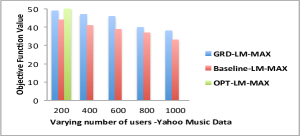
Number of users: We vary the number of users and use the default settings for the rest of the parameters. Figure 1 depicts the results. With increasing number of users, the objective function value decreases in general, because, more users typically introduce larger variation in the preference and smaller LM score. The results also clearly demonstrate that GRD-LM-MAX consistently outperforms Baseline-LM-MAX and achieves an objective function value comparable to OPT-LM-MAX.

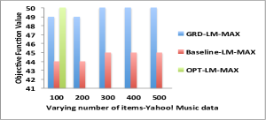
Number of items: Figure 1 shows that with increasing number of items, the objective function value typically increases. This is also intuitive, because, the top items of each group are likely to improve leading to higher LM score. Also, GRD-LM-MAX consistently outperforms the Baseline-LM-MAX.

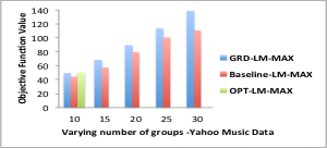
Number of groups: When number of groups is increased, the overall objective function value also increases. Notice that the objective function reaches its maximum possible value when number of groups equals the number of users. Therefore, with more groups, users get the flexibility to be with other users who are “similar” to them. Figure 1 presents these results. Similar to the above two cases, GRD-LM-MAX outperforms the baseline.

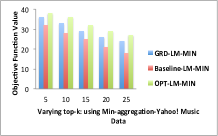
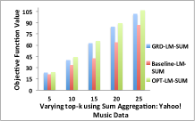
Top-$k$ on Min and Sum aggregation: In this experiment, we vary $k$ and produce the objective function value over the least preferred (i.e., bottom) item on the recommended top-$k$ item list. For Min-aggregation, Figure 2 shows that with increasing $k$, the objective function value decreases across the algorithms. This is natural, because, group satisfaction based on the bottom element typically decreases with increasing value of $k$. Figure 2 shows the Sum aggregation , where the objective function value increases across the algorithms with increasing $k$, although the rate of increase is smaller for higher $k$. These results demonstrate that GRD-LM algorithms are highly effective, their respective objective function values are quite comparable with that of OPT-LM.

7.1.2 Avg Group Satisfaction Over top-$k$ List

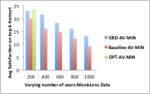
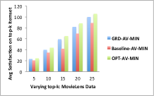
For lack of space, for this set of experiments, we only present the results on MovieLens dataset considering AV semantics. Here, we measure the average user satisfaction over all the recommended top-$k$ items, i.e., $\frac{\sum_{x=1}^{\ell}\sum_{j=1}^{k}\overline{sc(g_{x},i^{j})}}{\ell}$, where $\overline{sc(g_{x},i^{j})}$ is the average AV score on the $j$-th item for group $g_{x}$ using Min aggregation. While GRD-AV-MIN is not specifically optimized for this measure, our experimental results indicate that the formed groups have very high average satisfaction nevertheless.

Number of users: Figure 3 presents the results where we vary the number of users. Notice that for $10$ user groups, the maximum possible satisfaction per group over the top-$k$ item list could be as high as $25$ when $5$ items are recommended (and the ratings are in the scale of $1-5$). This is indeed true, because, $\sum_{j=1}^{5}\overline{sc(g,i^{j})}\leq 25$. Interestingly, GRD-AV-MIN consistently produces a score that is close to $25$ and outperforms the baseline algorithm.

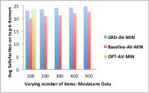
Number of items: When number of items is increased, the group satisfaction score is likely to increase, as the algorithms now have more options to recommend the top-$k$ items from, for each group. Figure 3 presents these results. The average group satisfaction score of both algorithms improves slightly with more items and again GRD-AV-MIN consistently beats the baseline.

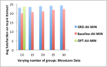
Number of groups: The results are shown in Figure 3. As expected, we observe that the aggregated group satisfaction over the top-$k$ items improves with the increasing number of groups. As explained before, with increasing number of groups, the algorithms have more flexibility to form groups with users who are highly similar in their top-$k$ item preferences.

Top-$k$ on Min-aggregation: Finally, we vary top-$k$ and compute the aggregated group satisfaction score over all top-$k$ items (results in Figure 3). With increasing $k$, the aggregation is done over more number of items, thus increasing the overall score. As shown in the figure, GRD-AV-MIN produces highly comparable results with that of OPT-AV-MIN and consistently outperforms the baseline algorithm Baseline-AV-MIN.

Figure 1: We measure the objective function value by varying # users, # items, # groups, respectively, one at a time. The default parameters are # users = $200$, # items = $100$, # groups = $10$, $k=5$ and Max-aggregation. The underlying dataset is Yahoo! Music.

Figure 2: We measure the objective function value by varying top-$k$ for Min and Sum-aggregation using Yahoo! Music. The default parameters are # users = $200$, # items = $100$, # groups = $10$, $k=5$.

Figure 3: We measure the average group satisfaction score on the top-$k$ item list $\frac{\sum_{x=1}^{\ell}\sum_{j=1}^{k}\overline{sc(g_{x},i^{j})}}{\ell}$ by varying # users, # items, # groups, and top-$k$, respectively, one at a time. The default parameters are # users = $200$, # items = $100$, # groups = $10$, $k=5$. The underlying dataset is MovieLens.

Figure 4: We present the average running time (measured in minutes) of the group formation algorithms under LM semantics with varying # users, # items, # groups respectively, one at a time. The default parameters are # users = $100,000$, # items = $10,000$, # groups = $10$, $k=5$, considering Min-aggregation. The underlying dataset is Yahoo! Music.

Figure 5: We present the average running time (measured in minutes) varying top-$k$, using Sum and Min aggregation for LM and AV. The default parameters are # users = $100,000$, # items = $10,000$, # groups = $10$. The underlying dataset is Yahoo! Music.

7.1.3 Distribution of Group Sizes

We randomly select $200$ users and $100$ items with the objective to form $\ell=10$ groups and recommend top-$k$ ($k=5$) items to each group using both datasets. In each sample of $200$ users, we measure the number of users in each of these $10$ groups. We repeat this experiment $3$ times and present the average variation in group size using a $5$-point summary : average minimum size, average 25% percentile (Q1), average median, average 75% percentile (Q3), average maximum size. This representation is akin to the box-plot summary [13]. The underlying algorithms are GRD-LM and GRD-AV considering both Max and Sum-aggregation. These results are summarized in Table 4. It is evident that the groups that are generated by our algorithms are balanced in general. Unsurprisingly, GRD-LM-MAX produces more uniform groups than GRD-LM-SUM, as the latter imposes stricter condition on grouping members (needs to match both top-$k$ sequence and ratings). Interestingly, notice that the generated group sizes have smaller average variation under AV than under LM. This is expected, because GRD-AV only requires users to have the same top-$k$ item sequence (irrespective of the specific ratings on the bottom item) to belong to the same group. Thus, AV tends to produce relatively larger groups and results in smaller variation in size across the generated groups.

Distribution of Average Group Size
Semantics	Quantile	GRD-*-MAX	GRD-*-SUM
LM	Minimum	$11.33$	$8.33$
	Q1	$15.75$	$11.5$
	Median	$18.5$	$13.66$
	Q3	$23.58$	$19.33$
	Maximum	$31.33$	$39.33$
AV	Minimum	$20.33$	$14.33$
	Q1	$22.4$	$19.35$
	Median	$25.4$	$22.5$
	Q3	$28.66$	$25.95$
	Maximum	$30.33$	$33.75$

Table 4: Distribution of Average Group Size

7.2 Scalability Experiments

For brevity, we present the results for only the larger dataset, Yahoo! Music, and present a subset of results. As mentioned earlier, OPT-LM and OPT-AV do not terminate beyond $200$ users, $100$ items, and $10$ groups, and are thus omitted. Our default settings here are as follows: number of users= $100,000$, number of items = $10,000$, number of groups =$10$, $k=5$ and Min-aggregation. Again, we vary # users, # items, # groups, and $k$.

Interpretation of Results: The running time of GRD is primarily affected by the number of users ($n$), number of groups ($\ell$), and $k$. Therefore, as it would be seen throughout the results, varying number of items does not impact the computational cost of either GRD-LM or GRD-AV. Between GRD-LM or GRD-AV, the latter takes more time, as it has to aggregate the satisfaction of all the users in a single group to produce the group satisfaction score. Running time of GRD-LM-MIN and GRD-LM-SUM are observed to be comparable, which corroborates our theoretical analysis. For the baseline algorithms (Baseline), running time increases with increasing number of users, and number of groups. Additionally, to produce the top-$k$ recommendations once the groups are formed, the last step of these algorithms has to sift through the item-ratings of all users inside every group. Given a group obtained using clustering, the ranked item lists of users may not be aligned. Thus, to form the group’s overall top-$k$ list, one may have to consider arbitrarily many items in the individual ranked items lists of the group members. Therefore, the computation time of the baseline algorithms increases with increasing $m$ or $k$. In case of our greedy algorithms, groups are formed by insisting that group members are aligned on the top-$k$ item sequence. Thus, forming the overall top-$k$ list for a group is straightforward in this case, for all groups but the $\ell$-th group formed by the greedy algorithms. For the $\ell$-th group, it sifts through the top-$k$ items per user to generate score.

7.2.1 Scalability Experiments : LM

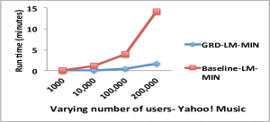
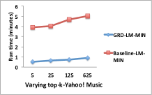
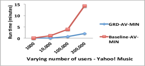
Number of users: We vary the number of users and measure the clock time of group formation and top-$k$ recommendation time for GRD-LM-MIN and Baseline-LM-MIN. (For the record, the optimal algorithms do not complete even after one hour.) Figure 4 presents the results in minutes. As expected, GRD-LM-MIN increases linearly and always terminates within $2$ minutes. These results also exhibit that the clustering based baseline algorithm is non-linear that our algorithm significantly outperforms.

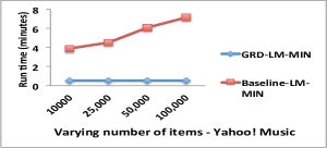
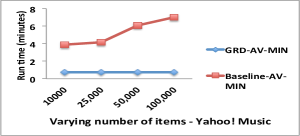
Number of items: Next, we vary the number of items and measure the clock time. As can be seen from Figure 4, the running time of our proposed algorithm is less affected by varying number of items. This result is also consistent with our theoretical analysis. Recall from Section 4.3 that the running time of both the algorithms is $O(nk+\ell\log n)$, which is independent of the number of items $m$. Since GRD-LM-MIN leverages the sorted top-$k$ list of items, more items do not necessarily lead to higher computational cost. On the contrary, the clustering based baseline has to produce the top-$k$ itemset for each user group once the groups are formed. As explained earlier, this requires considerable work since top-$k$ lists of cluster members may not be aligned. Figure 4 clearly demonstrates that Baseline-LM is rather sensitive to the increasing number of items. GRD-LM-MIN of course beats the baseline.

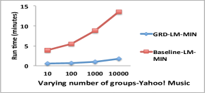
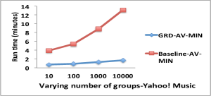
Number of groups: These results are presented in Figure 4. When the number of groups is increased, both Baseline-LM-MIN and our algorithm take more time. This observation is also consistent with our theoretical analyses, as the running time of both these algorithms depends on the number of groups. However, GRD-LM-MIN scales linearly with the increasing number of groups and outperform its baseline counterpart quite consistently.

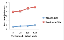
Top-$k$ on Min and Sum aggregation: We vary top-$k$ for both GRD-LM-MIN and Baseline-LM-MIN and present the running time in Figure 5. While GRD-LM-MIN consistently outperforms Baseline-LM-MIN, both these algorithms are not very sensitive to increasing $k$. The computation time of the first $\ell-1$ groups are not so much affected by $k$ and only determining the LM score and hence top-$k$ list of the last group (i.e., $\ell$-th group) is affected. The same observation holds for the baseline, as it incurs majority of its computations in forming the clusters that do not depend on $k$. Figure 5 presents the running time of both GRD-LM-SUM and Baseline-LM-SUM. GRD consistently outperforms Baseline, as expected, similar to Min aggregation.

7.2.2 Scalability Experiments : AV

Number of users: In this final set of scalability experiments, we again vary number of users and compute the running time of group formation algorithms under AV semantics. Figure 6 presents the results. These results are similar to those of LM, except that AV takes more time to compute than LM. Then, as expected, the running time of Baseline-AV is similar to that of Baseline-LM in Figure 4, as the clustering algorithm does not exploit the (AV) semantics in the group formation process. Our proposed greedy algorithm consistently outperforms the baseline algorithm.

Number of items: We vary the number of items and present the computation time in Figure 6. GRD-AV-MIN takes more time to terminate compared to that of GRD-LM-MIN (Figure 4), this slight increase is due to the extra computation that GRD-AV-MIN has to perform to aggregate AV score for each group. On the other hand, GRD-AV-MIN is not sensitive to the increasing number of items, similarly to GRD-LM-MIN. The figure clearly illustrates that Baseline-AV-MIN takes more time, as the number of items is increased. As usual, GRD outperforms Baseline.

Number of groups: We vary number of groups and observe that both algorithms incur higher processing time with increased number of groups. Figure 6 presents these results. As expected, GRD-AV-MIN scales linearly with the increasing number of groups and consistently outperforms the baseline algorithm.

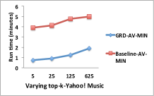
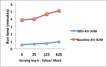
Top-$k$ on Min and Sum aggregation: We vary $k$ and measure the computation time in Figures 5 and Figure 5. With increased values of $k$, running time increases overall. However, GRD-AV-MIN takes significantly less time to terminate, compared to its baseline counterpart. Computation times of Baseline-LM-MIN and Baseline-AV-MIN are similar for the same values of $k$, as these baseline algorithms do not make use of the underlying group recommendation semantics during the group formation process. Sum aggregation results are presented in Figure 5 and the behavior is consistent, as before.

7.3 User Study

We use publicly available Flickr data to set up the user study in AMT for New York city. Given a Flickr log of a particular city, each row in that log corresponds to a user itinerary that is visited in a 12-hour window. From this log, we extract the most popular $10$ POIs. The user study is designed in two phases overall, where Phase 1 is used to create three different sets of users – similar, dissimilar, and random. Phase 2 is used to assess the performance of the algorithms on each of these sets, under different semantics and aggregation functions.

Phase 1: Preference Collection and Group Formation: First, we set up a HIT (Human Intelligence Task) in AMT, where we ask each AMT user to rate one of these $10$ POIs on a scale of $1-5$, higher rating implying greater preference. This data is collected from $50$ workers. From this collected dataset, we create user samples. Sampling is conducted to select a seed user.

Similar user sample: We select a subset of $10$ users who have provided very similar ranking on the $10$ POIs. We compute normalized pair-wise similarity, considering each item in the top-$10$ ranked item lists for each user pair and aggregating that over all $10$ items, as follows: $sim(u,u^{\prime})=\sum_{j=1}^{10}\frac{sim(u,u^{\prime},j)}{10}$

$$sim(u,u^{\prime},j) =\begin{cases}1-\frac{|sc(u,i^{j})-sc(u^{\prime},i^{j})|}{5}\text{ if }i_{j}^{u}=i_{j}^{u^{\prime}}\\ 0\text{\qquad otherwise}\end{cases}$$

Dissimilar user sample We select a different subset of $10$ users who has the smallest aggregate pair-wise similarity.
Random user sample In our third sample, we select another subset of $10$ users who are chosen randomly from the $50$ users (workers).

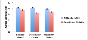
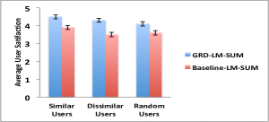
For brevity, we only report results on LM semantics for these experiments and set the number of groups to be $\ell=3$. We apply GRD-LM and Baseline-LM (both Sum and Min) to each sample and each algorithm produces three groups.

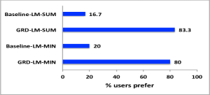
Step 2: Group Satisfaction Evaluation: In this phase, for each user sample (similar, dissimilar, and random), we set up $6$ HITs in AMT ($3$ for Min and another $3$ for Sum), where each HIT comprises the ($3+3$) groups created by GRD-LM and Baseline-LM. In each HIT, we first show the individual user preference ratings for all $10$ users in the sample, over all $10$ items. We do not disclose the underlying group formation algorithm (but refer to them as Method-1 and Method-2) and produce the groups formed by GRD-LM and Baseline-LM. We note that our settings mimic the set-up of previous user studies in group recommendation research [14, 1, 26]. We also request the worker to regard herself as one of the individuals in the sample and ask her to rate the following questions (higher is better): (1) Her satisfaction with the formed groups by Method-1; (2) Her satisfaction with the formed groups by Method-2, (3) In an absolute sense, which method she prefers more. Each HIT is undertaken by $10$ unique users, thereby involving $60$ new users in this phase ($30$ for Min and another $30$ for Sum). For each HIT, we average the ratings and present them in Figures 7 and 7. Standard error bars are added for statistical significance.

Additionally, we aggregate and compute the percentage of users who prefer GRD-LM versus Baseline-LM in Figure 7.

Interpretation of Results: We make the following key observations from the results presented in Figures 7, 7, 7. First and foremost, our proposed algorithm GRD-LM gives rise to higher satisfaction compared to the baseline, in all cases. In fact, this difference in satisfaction seems to be higher when the user population is dissimilar in its individual preferences. During our post-analysis, we see, indeed the clustering based baseline algorithm becomes ineffective, when the individual user preferences are dissimilar from each other. For the same reason, the difference in the average satisfaction of our greedy algorithm from the baseline algorithm is the highest for dissimilar users and smallest for similar users. A random user population consists of both similar and dissimilar users, hence the effectiveness falls in the middle. These results clearly demonstrate that our proposed solutions can effectively exploit existing group recommendation semantics and form groups that lead to high group satisfaction in practice.

Figure 6: We present the average running time (measured in minutes) of the group formation algorithms under AV semantics with varying # users, # items, # groups respectively, one at a time. The default parameters are # users = $100,000$, # items = $10,000$, # groups = $10$, $k=5$, considering Min-aggregation. The underlying dataset is Yahoo! Music.

Figure 7: User Study Results: Figures 7 and 7 present the average user satisfaction score of GRD-LM and that of Baseline-LM for both Min and Sum aggregation with statistical significance analyses. Figure 7 indicates about 80% of the users prefers GRD over the Baseline algorithms.

8 Related Work

While no prior work has addressed the problem of group formation in the context of recommender systems, we still discuss existing work that appears to be contextually most related.

Group Recommendation: Group recommendation has been designed for various domains such as news pages [24], tourism [11], music [9], book, restaurants [22], and TV programs [31].

There are two dominant strategies for group recommendations [8, 1]. The first approach creates a pseudo-user representing the group and then makes recommendations to that pseudo-user, while the second strategy computes a recommendation list for each group member and then combines them to produce a group’s list. For the latter, a widely adopted approach is to apply an aggregation function to obtain a consensus group preference for a candidate item. Popular aggregation functions, such as, least misery, aggregate voting are popularly used in existing works [14, 1, 26].  [22] pre-clusters the users and the individual recommendations are generated for group members using that member’s cluster. After that group aggregation function is applied.

In these works, groups are created beforehand, either by a random set of users with different interests, or by a number of users who explicitly choose to be part of a group.

Market-based Strategies: Existing research on market based strategies [6, 18, 20] studies problems on daily deals sites, such as Groupon and LivingSocial, that are orthogonal to our group formation problem. These works focus on recommending deals (i.e., items) to the users and groups For example, [18] proposes new algorithms for daily deals recommendation based on the explore-then-exploit strategy. [20] recommends the best deals to the users, among a set of candidate deals, to maximize revenues. Real-time bidding strategy for group-buying deals based on the online optimization of bid values is studied in [6]. This body of works essentially relies on price discounts to incentivize group formation around deals, with the objective of maximizing revenue. By contrast, we investigate how to form groups to maximize user satisfaction under existing group recommendations semantics. Our work is directly deployable as a non-intrusive addition to group recommender systems where explicit incentives may not be present.

Team Formation: Team formation problems  [19, 7, 33, 3, 4] are often modeled using Integer Programming, or heuristic solutions using Simulated Annealing [7] or Genetic Algorithms [29] are designed. These problems are assignment problems.

In general, group formation is not a matching or generalized assignment problem [17, 10]. There are no resources to match the users to. We need to “match” users to one another. In that sense, it’s closer in spirit to clustering [13]. However, as we demonstrate in the paper, a clustering algorithm which is agnostic to the group recommendation semantics (LM or AV) is likely to perform poorly for purposes of maximizing group satisfaction.

Community Detection: These problems [28] discover communities (a set of users) with common interests. Again, our groups have a more explicit connotation (in the sense of having clearly defined satisfaction scores) than communities. One can potentially generate a graph of users based on a suitable notion of distance or similarity between users in terms of tastes and find communities. Once again, this approach falls short, as it does not take group recommendation semantics into account.

Multi-way Partition: Minimization problems over multiway partition functions are studied in  [32, 2], with graphs or hyper-graphs as the underlying abstract model. They attempt to partition the nodes to optimize certain outcome (e.g., variants of $k$-cut problems). While these problems are NP-hard, efficient algorithms with provable approximation factors are known, when the objective function exhibit certain properties [32, 2]. If we are to use such a weighted graph, the weight on each edge is local to just two users and does not capture the essence of group recommendation semantics, which renders those solutions to our problem far from ideal.

9 Conclusion

We initiate the study of forming groups in the context of group recommender systems. We consider two popular group recommendation semantics (LM and AV) and formalize the problem of creating a set of non-overlapping groups over an underlying user population, such that the aggregate satisfaction of the formed groups, with their recommended top-$k$ lists, is maximized. We prove that optimal group formation is computationally intractable under both group recommendation semantics. We present efficient greedy group formation algorithms and show that they achieve absolute error guarantees for LM. We present a comprehensive experimental analysis and user studies that demonstrates the effectiveness as well scalability of our proposed solutions.

The approximability of group formation under AV semantics remains open although we conjecture that it may be hard to approximate. Identifying natural special cases that are tractable is an interesting open problem. Forming groups where the individual members are not treated equally, or groups that are possibly overlapping are also worthy of study.

Appendix A Optimal Algorithms

Despite the fact that the optimal group formation problem is computationally intractable, we describe optimal algorithms under both LM and AV semantics by formulating them as integer programming problems. We can make use of existing integer programming solvers (such as CPLEX) to solve these problems. Since IP is also NP-hard [30] and could be exponential in the worst case, the proposed solutions are not scalable. Nevertheless, the formulation is useful when the numbers of users and items are fairly small.

For both formulations the following Boolean decision variables are defined: $u_{ig}$ captures whether user $u_{i}$ is part of group $g$. To describe the top-$k$ itemset of each group, an additional Boolean decision variable, $y_{jg}$ checks, if item $j$ is the $k$-th item for group $g$, whereas, $w_{jg}$ is used to check if item $j$ is one of the top-$(k-1)$ items for group $g$. The following formulation is provided assuming Min-aggregation for a general value of $k>1$. To consider Max-aggregation formulation, we no longer need $w_{jp}$ and one has to check if $y_{jg}$ is indeed the top-$1$ item for the recommended itemset. Similarly, Sum aggregation could be performed by modifying the objective function to aggregate over all $k$-items.

A.1 IP Formulation for Least Misery

The objective function for LM aims to form $\ell$ groups such that their sum of scores is maximized. The first two constraints capture the fact that the score of an item $j$ is to be computed by considering the minimum score of that item over all users. The third and fourth constraints are used to capture the top-$(k-1)$ items. The rest of the constraints simply state that the $k-$th item is a single item for every group, whereas, there should be a total of $k-1$ additional items whose score is higher than that of the $k$-th item. Finally, we assert that only $\ell$ groups are to be formed, whereas, a user can belong to only one of these groups (satisfying disjointness).

$$\text{Maximize }\Sigma_{g=1}^{\ell}\{y_{jp}\times sc(g,j)\}$$ (1)

s.t.

$$\left.\begin{aligned} sc(j,g)=r\\ r\leq{{\{\forall u_{ig}=1\}}}u_{ig}\times sc(u_{i},j)\\ w_{ig}\times sc(g,i)\geq y_{jg}\times sc(g,j)\times w_{ig}\\ (1-w_{jg})\times sc(g,j)\leq y_{jg}\times sc(g,j)\\ \end{aligned}\right\}$$

$$\left.\begin{aligned} \Sigma_{j=1}^{m}y_{jg}=1\\ \Sigma_{i=1}^{m}w_{ig}=k-1\\ \ell\leq n\\ \end{aligned}\right\}$$

$$\left.\begin{aligned} y_{jg}=1/0,\forall j=1,2,\ldots,m\\ w_{jg}=1/0,\forall j=1,2,\ldots,m\\ \Sigma_{g=1}^{\ell}u_{ig}=1,\forall i=1,2,\ldots,n\\ u_{ig}=1/0,\forall i=1,2,\ldots,n,\forall g=1,2,\ldots,\ell\\ \end{aligned}\right\}$$

When this IP is run on Example 1, considering $k=1$, the following groups are produced: $\{u_{1},u_{3},u_{4}\}$, $\{u_{2},u_{6}\}$, $\{u_{5}\}$ with an overall $Obj$ value of $4+5+3=12$.

A.2 IP Formulation for Aggregate Voting

The formulation of optimal group formation under aggregate voting is similar to that of LM, except for the fact that the score of an item $j$ for a group $g$ is the summation of scores of $j$ over all users in $g$.

$$\text{Maximize }\Sigma_{p=1}^{\ell}\{y_{jg}\times sc(g,j)\}$$ (2)

s.t.

$$\left.\begin{aligned} sc(g,j)=\Sigma_{{\{\forall u_{ig}=1\}}}u_{ig}\times sc(u_{i},j)\\ w_{ig}\times sc(g,i)\geq y_{jg}\times sc(g,j)\times w_{ig}\\ (1-w_{jg})\times sc(g,j)\leq y_{jp}\times sc(g,j)\\ \end{aligned}\right\}$$

$$\left.\begin{aligned} \Sigma_{j=1}^{m}y_{jg}=1\\ \Sigma_{i=1}^{m}w_{ig}=k-1\\ \ell\leq n\\ \end{aligned}\right\}$$

$$\left.\begin{aligned} y_{jg}=1/0,\forall j=1,2,\ldots,m\\ w_{jg}=1/0,\forall j=1,2,\ldots,m\\ \Sigma_{g=1}^{\ell}u_{ig}=1,\forall i=1,2,\ldots,n\\ u_{ig}=1/0,\forall i=1,2,\ldots,n,\forall g=1,2,\ldots,\ell\\ \end{aligned}\right\}$$

When run on Example 2, the optimal grouping with two groups consists of the following groups: $\{u_{1},u_{3},u_{4}\}$, and $\{u_{2},u_{5},u_{6}\}$, with the overall objective function value of $14$.

Appendix B Suboptimal Group Formation by GRD-LM-SUM

Example B.11.

Consider the user set
$\mathcal{U}=\{u_{1},u_{2},u_{3},u_{4},u_{5},u_{6}\}$ and the itemset $\mathcal{I}=\{i_{1},i_{2},i_{3}\}$. The users’ preferences for the itemset are given (or predicted) as in Table 5. Suppose the users need to be partitioned into at most $3$ groups ($\ell\leq 3$), where each group has to be recommended $k=2$ items. ∎

Using GRD-LM-SUM, this will form the following $3$ groups at the end: $\{u_{2}\}$, $\{u_{3},u_{4}\}$, $\{u_{1},u_{5},u_{6}\}$ with the overall objective function value as $(5+3)+(5+2)+(3+2)=20$, whereas, the optimal grouping will give a different solutions to form $3$ groups, $\{u_{2},u_{6}\}$, $\{u_{3},u_{4}\}$, $\{u_{1},u_{5}\}$ with the overall objective function value of $(5+2)+(5+2)+(4+3)=21$.

User-item Ratings	$u_{1}$	$u_{2}$	$u_{3}$	$u_{4}$	$u_{5}$	$u_{6}$
$i_{1}$	1	2	2	2	2	1
$i_{2}$	4	3	5	5	4	2
$i_{3}$	3	5	1	1	3	5

Table 5: User Item Preference Rating for Example B.11

References

- [1] S. Amer-Yahia, S. B. Roy, A. Chawla, G. Das, and C. Yu. Group recommendation: Semantics and efficiency. PVLDB, 2(1):754–765, 2009.
- [2] O. Amini, F. Mazoit, N. Nisse, and S. Thomassé. Submodular partition functions. Discrete Mathematics, 309(20):6000–6008, 2009.
- [3] A. Anagnostopoulos, L. Becchetti, C. Castillo, A. Gionis, and S. Leonardi. Power in unity: forming teams in large-scale community systems. In Proceedings of the 19th ACM international conference on Information and knowledge management, pages 599–608. ACM, 2010.
- [4] A. Anagnostopoulos, L. Becchetti, C. Castillo, A. Gionis, and S. Leonardi. Online team formation in social networks. In Proceedings of the 21st international conference on World Wide Web, pages 839–848. ACM, 2012.
- [5] R. Baeza-Yates, B. Ribeiro-Neto, et al. Modern information retrieval, volume 463. ACM press New York, 1999.
- [6] R. Balakrishnan and R. P. Bhatt. Real-time bid optimization for group-buying ads. In Proceedings of the 21st ACM international conference on Information and knowledge management, pages 1707–1711. ACM, 2012.
- [7] A. Baykasoglu, T. Dereli, and S. Das. Project team selection using fuzzy optimization approach. Cybernetics and Systems: An International Journal, 38(2):155–185, 2007.
- [8] S. Berkovsky and J. Freyne. Group-based recipe recommendations: analysis of data aggregation strategies. In RecSys, pages 111–118, 2010.
- [9] A. Crossen, J. Budzik, and K. J. Hammond. Flytrap: intelligent group music recommendation. In Proceedings of the 7th international conference on Intelligent user interfaces, pages 184–185. ACM, 2002.
- [10] L. Fleischer, M. X. Goemans, V. S. Mirrokni, and M. Sviridenko. Tight approximation algorithms for maximum general assignment problems. In Proceedings of the seventeenth annual ACM-SIAM symposium on Discrete algorithm, pages 611–620. ACM, 2006.
- [11] I. Garcia, L. Sebastia, and E. Onaindia. On the design of individual and group recommender systems for tourism. Expert Syst. Appl., 38(6):7683–7692, 2011.
- [12] M. R. Garey and D. S. Johnson. Computers and Intractability: A Guide to the Theory of NP-Completeness. 1979.
- [13] J. Han and M. Kamber. Data Mining: Concepts and Techniques. Morgan Kaufmann, 2000.
- [14] A. Jameson and B. Smyth. Recommendation to groups. In The adaptive web, pages 596–627. Springer, 2007.
- [15] V. Kann. Maximum bounded 3-dimensional matching is max snp-complete. Information Processing Letters, 37(1):27–35, 1991.
- [16] V. Kann. On the approximability of NP-complete optimization problems. PhD thesis, Royal Institute of Technology Stockholm, 1992.
- [17] S. O. Krumke and C. Thielen. The generalized assignment problem with minimum quantities. European Journal of Operational Research, 228(1):46–55, 2013.
- [18] A. Lacerda, A. Veloso, and N. Ziviani. Exploratory and interactive daily deals recommendation. In RecSys, 2013.
- [19] T. Lappas, K. Liu, and E. Terzi. Finding a team of experts in social networks. In SIGKDD, pages 467–476, 2009.
- [20] T. Lappas and E. Terzi. Daily-deal selection for revenue maximization. In 21st ACM International Conference on Information and Knowledge Management, CIKM’12, Maui, HI, USA, October 29 - November 02, 2012, pages 565–574, 2012.
- [21] H. Lieberman, N. Van Dyke, and A. Vivacqua. Let’s browse: a collaborative browsing agent. Knowledge-Based Systems, 12(8):427–431, 1999.
- [22] E. Ntoutsi, K. Stefanidis, K. Nørvåg, and H.-P. Kriegel. Fast group recommendations by applying user clustering. In ER, pages 126–140, 2012.
- [23] M. O’connor, D. Cosley, J. A. Konstan, and J. Riedl. Polylens: a recommender system for groups of users. In ECSCW 2001, pages 199–218. Springer, 2001.
- [24] S. Pizzutilo, B. De Carolis, G. Cozzolongo, and F. Ambruoso. Group modeling in a public space: Methods, techniques, experiences. In Proceedings of the 5th WSEAS International Conference on Applied Informatics and Communications, AIC’05, pages 175–180, Stevens Point, Wisconsin, USA, 2005. World Scientific and Engineering Academy and Society (WSEAS).
- [25] C. Romesburg. Cluster analysis for researchers. Lulu. com, 2004.
- [26] S. B. Roy, S. Thirumuruganathan, S. Amer-Yahia, G. Das, and C. Yu. Exploiting group recommendation functions for flexible preferences. In ICDE Conference, 2014.
- [27] C. Senot, D. Kostadinov, M. Bouzid, J. Picault, A. Aghasaryan, and C. Bernier. Analysis of strategies for building group profiles. In User Modeling, Adaptation, and Personalization, pages 40–51. Springer, 2010.
- [28] M. Sozio and A. Gionis. The community-search problem and how to plan a successful cocktail party. In Proceedings of the 16th ACM SIGKDD international conference on Knowledge discovery and data mining, pages 939–948. ACM, 2010.
- [29] H. Wi, S. Oh, J. Mun, and M. Jung. A team formation model based on knowledge and collaboration. Expert Systems with Applications, 36(5):9121–9134, 2009.
- [30] L. A. Wolsey. Integer programming, volume 42. Wiley New York, 1998.
- [31] Z. Yu, X. Zhou, Y. Hao, and J. Gu. TV Program Recommendation for Multiple Viewers Based on user Profile Merging. User Modeling and User-adapted Interaction, 16:63–82, 2006.
- [32] L. Zhao, H. Nagamochi, and T. Ibaraki. Greedy splitting algorithms for approximating multiway partition problems. Mathematical Programming, 102(1):167–183, 2005.
- [33] A. Zzkarian and A. Kusiak. Forming teams: an analytical approach. IIE transactions, 31(1):85–97, 1999.