Evaluation techniques for Gutzwiller wave functions in finite dimensions

Abstract

We give a comprehensive introduction into a diagrammatic method that allows for the evaluation of Gutzwiller wave functions in finite spatial dimensions. We discuss in detail some numerical schemes that turned out to be useful in the real-space evaluation of the diagrams. The method is applied to the problem of d-wave superconductivity in a two-dimensional single-band Hubbard model. Here, we discuss in particular the role of long-range contributions in our diagrammatic expansion. We further reconsider our previous analysis on the kinetic energy gain in the superconducting state.

1 Introduction

For the study of the ground-state properties of quantum systems, variational wave functions can be a powerful tool. The most common variational approach in the theory of correlated electron systems is the Hartree–Fock approximation (HFA) which is based on (variational) single-particle product wave functions $|\Psi_{0}\rangle$. If applied to systems with attractive, e.g., phonon-mediated interactions, the HF theory leads to the celebrated BCS theory on superconductivity [1].

The crucial first step in any variational approach is the calculation of the energy expectation value for a given class of variational wave functions. For HF wave functions this can always be achieved by means of Wick’s theorem, which explains the popularity of this approach. Many phenomena in correlated electron systems, however, cannot be described properly by the HFA, especially, in (effectively) one- or two-dimensional systems. This holds, in particular, for unconventional superconductivity which has been observed in a number of materials, such as Cuprates, Ruthenates and iron-based Pnictides.

A way to improve the HFA is based on ‘Jastrow wave functions’ which have the form [2, 3]

$$|\Psi_{\rm J}\rangle=\hat{P}_{\rm J}|\Psi_{0}\rangle\;.$$ (1)

Here, $\hat{P}_{\rm J}$ is an operator which has been chosen in various ways in the literature [4, 5, 6, 7, 8, 9, 10] and is meant to account for correlation effects which are not captured by the Hartree–Fock (single-particle) wave function $|\Psi_{0}\rangle$. One of the simplest examples for such a Jastrow wave function is the Gutzwiller wave function [4, 5, 6] which will be used in this work.

Evaluating expectation values for Jastrow (or Gutzwiller) wave functions is a difficult many-particle problem which, in general, can only by tackled by numerical techniques, such as the ‘variational Monte-Carlo method’ (VMC) [11, 12, 13]. We have recently developed a diagrammatic scheme for the evaluation of expectation values for Gutzwiller wave functions. Unlike the VMC, our method adresses the infinite systems and, hence, it does not suffer from the typical finite-size errors of VMC. As shown in Ref. [14] , our approach allows us to study e.g., the stability of nematic (‘Pomeranchuk’) phases in two-dimensional Hubbard models. First results on the stability of superconducting ground states in these models have been presented in Ref. [15].

In this work we will give a comprehensive introduction into the technical details of our approach for the study of superconducting ground states and present numerical results which complement those published in previous work, Refs. [14, 15, 16, 17, 18]. We will introduce, in particular, a new way to evaluate diagrams which contain long-range correlations.

Our presentation is organised as follows. In Section 2 we introduce the diagrammatic method which we use for the investigation of the single-band model. The class of diagrams which requires a special treatment due to their long-range contributions is discussed in Section 3. In Section 4 we show numerical results and focus, in particular, on the convergence of our diagrammatic scheme. Our presentation is closed by a Summary and Outlook in Section 5. Some technical parts of the presentation are referred to three appendices

2 Model and Method

We investigate the single-band Hubbard model

$$\hat{H}=\hat{H}_{0}+U\sum_{{\bf i}}\hat{d}_{{\bf i}}\,,$$ (2)

in two dimensions, where

$$\hat{H}_{0}=\sum_{{\bf i},{\bf j},\sigma}t_{{\bf i},{\bf j}}\hat{c}_{{\bf i},\sigma}^{\dagger}\hat{c}_{{\bf j},\sigma}^{\phantom{\dagger}}\,\,\,,\,\,\,\hat{d}_{{\bf i}}\equiv\hat{n}_{{\bf i},\uparrow}\hat{n}_{{\bf i},\downarrow}\,.$$ (3)

Here, ${\bf i}=(i_{1},i_{2})$ denotes one of the $L$ sites on a square lattice, and $\sigma=\uparrow,\downarrow$. The properties of this model will be studied in the thermodynamic limit $L\to\infty$ by means of the variational wave functions

$$|\Psi_{\rm G}\rangle=\hat{P}_{\rm G}|\Psi_{0}\rangle=\prod_{{\bf i}}\hat{P}_{{\bf i};{\rm G}}|\Psi_{0}\rangle\;,$$ (4)

first introduced by Gutzwiller [4], where $|\Psi_{0}\rangle$ is a (normalised) single-particle product state and the local ‘Gutzwiller correlator’ is defined by

$$\hat{P}_{{\bf i}}=\sum_{\Gamma}\lambda_{\Gamma}|\Gamma\rangle_{{\bf i}\,{\bf i}}\!\langle\Gamma|\;.$$ (5)

It contains the variational parameters $\lambda_{\Gamma}$ for the four local states

$$|\Gamma\rangle_{{\bf i}}\in\left\{|\emptyset\rangle_{{\bf i}},|\uparrow\rangle_{{\bf i}},|\downarrow\rangle_{{\bf i}},|\uparrow\downarrow\rangle_{{\bf i}}\right\}$$ (6)

for the empty, singly, or doubly occupied site ${\bf i}$. Note that in Eq. (5) we have already assumed a translationally invariant ground state which allows us to work with parameters $\lambda_{\Gamma}$ that do not depend on the lattice site ${\bf i}$.

The single particle state $|\Psi_{0}\rangle$ is also a variational object and may be chosen as the ground state of an effective single-particle Hamiltonian,

$$\hat{H}_{0}^{\rm eff}=\sum_{{\bf i},{\bf j},\sigma}t^{\rm eff}_{{\bf i},{\bf j}}\hat{c}_{{\bf i},\sigma}^{\dagger}\hat{c}_{{\bf j},\sigma}^{\phantom{\dagger}}+\sum_{{\bf i}\neq{\bf j}}\bigl{(}\Delta^{\rm eff}_{{\bf i},{\bf j}}\hat{c}_{{\bf i},\uparrow}^{\dagger}\hat{c}_{{\bf j},\downarrow}^{\dagger}+{\rm h.c.}\bigr{)}\;.$$ (7)

The effective hopping and pairing parameters $t^{\rm eff}_{{\bf i},{\bf j}}$ and $\Delta^{\rm eff}_{{\bf i},{\bf j}}$ can then be considered as variational parameters which determine $|\Psi_{0}\rangle$. Note that, in the main part of this work, we will consider superconducting ground states with $d$-wave symmetry for which the local pairing amplitude vanishes,

$$\langle\hat{c}^{(\dagger)}_{{\bf i},\uparrow}\hat{c}^{(\dagger)}_{{\bf i},\downarrow}\rangle_{0}=\langle\hat{c}^{(\dagger)}_{{\bf i},\uparrow}\hat{c}^{(\dagger)}_{{\bf i},\downarrow}\rangle_{\rm G}=0\;.$$ (8)

Here we introduced the notation $\langle\ldots\rangle_{0,{\rm G}}$ for expectation values with respect to $|\Psi_{0}\rangle$ and $|\Psi_{\rm G}\rangle$. The case of a finite local pairing (8) is discussed in Appendix A.

2.1 Diagrammatic expansion

We need to evaluate the expectation value of the Hamiltonian (2),

$$E_{\rm G}\equiv\sum_{{\bf i},{\bf j},\sigma}t_{{\bf i},{\bf j}}\frac{\langle\Psi_{\rm G}|\hat{c}_{{\bf i},\sigma}^{\dagger}\hat{c}_{{\bf j},\sigma}^{\phantom{\dagger}}|\Psi_{\rm G}\rangle}{\langle\Psi_{\rm G}|\Psi_{\rm G}\rangle}+U\sum_{{\bf i}}\frac{\langle\Psi_{\rm G}|\hat{d}_{{\bf i}}|\Psi_{\rm G}\rangle}{\langle\Psi_{\rm G}|\Psi_{\rm G}\rangle}\;,$$ (9)

with respect to our Gutzwiller wave function (4). As first shown in Ref. [14], we can develop an efficient diagrammatic scheme for this evaluation if we demand that

$$\hat{P}_{{\bf l}}^{\dagger}\hat{P}_{{\bf l}}=\hat{P}^{2}_{{\bf l}}=1+x\hat{d}_{{\bf l}}^{\rm HF}\;,$$ (10)

where

$$\hat{d}_{{\bf l}}^{\rm HF}\equiv\hat{n}^{\rm HF}_{{\bf l},\uparrow}\hat{n}^{\rm HF}_{{\bf l},\downarrow}\;\;,\;\;\hat{n}^{\rm HF}_{{\bf l},\sigma}\equiv\hat{n}_{{\bf l},\sigma}-n_{0}\;,$$ (11)

and $n_{0}\equiv\langle\hat{n}_{{\bf l},\sigma}\rangle_{0}=N/(2L)$. Equation (10) determines three of the four parameters $\lambda_{\Gamma}$ as well as the coefficient $x$. In this way, we are left with only one variational parameter. For instance, we may express the parameters $\lambda_{\Gamma}$ by the coefficient $x$,

$$\lambda^{2}_{d} = 1+x(1-n_{0})^{2}\;,$$ (12)

$$\lambda^{2}_{\sigma} = 1-xn_{0}(1-n_{0})\;,$$ (13)

$$\lambda^{2}_{\emptyset} = 1+xn_{0}^{2}\;.$$ (14)

For the calculation of (9) we need to evaluate three power series in $x$,

$$\langle\Psi_{\rm G}|\Psi_{\rm G}\rangle = \sum_{k=0}^{\infty}\frac{x^{k}}{k!}\sideset{}{{}^{\prime}}{\sum}_{{\bf l}_{1},\ldots{\bf l}_{k}}\bigl{\langle}\hat{d}^{\rm HF}_{{\bf l}_{1},\ldots,{\bf l}_{k}}\bigr{\rangle}_{0}\,,$$ (15)

$$\langle\Psi_{\rm G}|\hat{d}_{{\bf i}}^{\vphantom{\rm HF}}|\Psi_{\rm G}\rangle = \lambda_{d}^{2}\sum_{k=0}^{\infty}\frac{x^{k}}{k!}\sideset{}{{}^{\prime}}{\sum}_{{\bf l}_{1},\ldots{\bf l}_{k}}\bigl{\langle}\hat{d}_{{\bf i}}^{\vphantom{\rm HF}}\hat{d}^{\rm HF}_{{\bf l}_{1},\ldots,{\bf l}_{k}}\bigr{\rangle}_{0}\,,$$ (16)

$$\langle\Psi_{\rm G}|\hat{c}^{\dagger}_{{\bf i},\sigma}\hat{c}_{{\bf j},\sigma}^{\phantom{\dagger}}|\Psi_{\rm G}\rangle = \sum_{k=0}^{\infty}\frac{x^{k}}{k!}\sideset{}{{}^{\prime}}{\sum}_{{\bf l}_{1},\ldots{\bf l}_{k}}\bigl{\langle}\widetilde{c}_{{\bf i},\sigma}^{\dagger}\widetilde{c}_{{\bf j},\sigma}^{\phantom{\dagger}}\hat{d}^{\rm HF}_{{\bf l}_{1},\ldots,{\bf l}_{k}}\bigr{\rangle}_{0}\,,$$ (17)

where we used Eq. (10) and introduced the notation

$$\hat{d}^{\rm HF}_{{\bf l}_{1},\ldots,{\bf l}_{k}} \equiv \hat{d}^{\rm HF}_{{\bf l}_{1}}\cdots\hat{d}^{\rm HF}_{{\bf l}_{k}}\quad,\quad\hat{d}^{\rm HF}_{\emptyset}\equiv 1\;,$$ (18)

$$\widetilde{c}_{{\bf i},\sigma}^{(\dagger)} \equiv \hat{P}_{{\bf i}}\hat{c}^{(\dagger)}_{{\bf i},\sigma}\hat{P}_{{\bf i}}\;.$$ (19)

The primes in Eqs. (15)–(17) indicate the summation restrictions

$${\bf l}_{p}\neq{\bf l}_{p^{\prime}}\;,\;\;{\bf l}_{p}\neq{\bf i},{\bf j}\;\;\;\;\;\;\forall p,p^{\prime}\;.$$ (20)

The expectation values $\langle\ldots\rangle_{0}$ in (15)-(17) can be evaluated by means of Wick’s theorem [19]. In the resulting diagrammatic expansion, the $k$th-order terms correspond to diagrams with $k$ ‘internal’ vertices on sites ${\bf l}_{1},\ldots,{\bf l}_{k}$, one (two) ‘external’ vertices on site ${\bf i}$ (${\bf i}$ and ${\bf j}$) and lines

$$P^{\sigma}_{{\bf l},{\bf l}^{\prime}} \equiv \langle\hat{c}^{\dagger}_{{\bf l},\sigma}\hat{c}_{{\bf l}^{\prime},\sigma}^{\phantom{\dagger}}\rangle_{0}\;,$$ (21)

$$S_{{\bf l},{\bf l}^{\prime}} \equiv \langle\hat{c}^{\dagger}_{{\bf l},\uparrow}\hat{c}^{\dagger}_{{\bf l}^{\prime},\downarrow}\rangle_{0}=\langle\hat{c}_{{\bf l}^{\prime},\downarrow}\hat{c}_{{\bf l},\uparrow}\rangle^{*}_{0}$$ (22)

connecting these vertices. By construction, we eliminated all diagrams with local ‘Hartree bubbles’ at internal vertices, i.e., diagrams with lines that leave and enter the same internal vertex. To achieve the same for the external vertices in (16),(17) we rewrite the corresponding operators as

$$\hat{d}_{{\bf i}} = (1-xd_{0})\hat{d}^{\rm HF}_{{\bf i}}+n_{0}(\hat{n}^{\rm HF}_{{\bf i},\uparrow}+\hat{n}^{\rm HF}_{{\bf i},\downarrow})+d_{0}\hat{P}^{2}_{{\bf i}}\;,$$ (23)

$$\widetilde{c}_{{\bf i},\sigma}^{(\dagger)} = q\hat{c}^{(\dagger)}_{{\bf i},\sigma}+\alpha\hat{c}^{(\dagger)}_{{\bf i},\sigma}\hat{n}^{\rm HF}_{{\bf i},\bar{\sigma}}\;,$$ (24)

where we introduced

$$d_{0} \equiv n_{0}^{2}\;,$$ (25)

$$q \equiv \lambda_{1}(\lambda_{d}n_{0}+\lambda_{\emptyset}(1-n_{0}))\;,$$ (26)

$$\alpha \equiv \lambda_{1}(\lambda_{d}-\lambda_{\emptyset})\;,$$ (27)

and $\bar{\uparrow}=\downarrow$, $\bar{\downarrow}=\uparrow$. When inserted into (16), the last term in (23) combines to $\lambda_{d}^{2}d_{0}\langle\Psi_{\rm G}|\Psi_{\rm G}\rangle$ so that it does not have to be evaluated diagrammatically.

As a result, we obtain diagrammatic sums with no Hartree bubbles at any vertex. This allows us to replace the lines (21) by

$$\bar{P}^{\sigma}_{{\bf l},{\bf l}^{\prime}}\equiv\langle\hat{c}^{\dagger}_{{\bf l},\sigma}\hat{c}_{{\bf l}^{\prime},\sigma}^{\phantom{\dagger}}\rangle_{0}-\delta_{{\bf l},{\bf l}^{\prime}}n_{0}\;.$$ (28)

As demonstrated in Ref. [14], the elimination of Hartree bubbles has significant consequences for the convergence and, hence, accuracy of our diagrammatic expansion. Due to our assumption of d-wave superconductivity, we do not have to eliminate ‘anomalous’ Hartree bubbles of the form (8). In Appendix A we explain how our diagrammatic method can be generalised if Eq. (8) is not fulfilled.

As the final analytical step of our derivation, we apply the linked-cluster theorem [19]. The norm (15) cancels the disconnected diagrams in the two numerators (16) and (17). Note that for the application of this theorem, we first need to lift the summation restrictions in Eqs. (15)-(17). This can be done, however, without generating additional terms, as we explain in Appendix B.

For a translationally invariant system, the remaining task is to evaluate the diagrammatic sums

$$S=\sum_{k=0}^{\infty}\frac{x^{k}}{k!}S(k)$$ (29)

with

$$S\in\Big{\{}I^{(2)},I^{(4)},T^{(1),(1)}_{{\bf i},{\bf j}},T^{(1),(3)}_{{\bf i},{\bf j}},T^{(3),(1)}_{{\bf i},{\bf j}},T^{(3),(3)}_{{\bf i},{\bf j}}\Big{\}}$$ (30)

and

$$I^{(2)[(4)]}(k)\equiv\sum_{{\bf l}_{1},\ldots,{\bf l}_{k}}\bigl{\langle}\hat{n}^{\rm HF}_{{\bf i},\sigma}[\hat{d}^{\rm HF}_{{\bf i}}]\hat{d}^{\rm HF}_{{\bf l}_{1},\ldots,{\bf l}_{k}}\bigr{\rangle}^{\rm c}_{0}\;,$$ (31)

$$T_{{\bf i},{\bf j}}^{(1)[(3)],(1)[(3)]}(k)$$

$$\equiv\sum_{{\bf l}_{1},\ldots,{\bf l}_{k}}\bigl{\langle}[\hat{n}^{\rm HF}_{{\bf i},\bar{\sigma}}]\hat{c}^{\dagger}_{{\bf i},\sigma}[\hat{n}^{\rm HF}_{{\bf j},\bar{\sigma}}]\hat{c}_{{\bf j},\sigma}^{\phantom{\dagger}}\hat{d}^{\rm HF}_{{\bf l}_{1},\ldots,{\bf l}_{k}}\rangle^{\rm c}_{0}\;.$$ (32)

Here, $\langle\dots\rangle_{0}^{\rm c}$ indicates that only connected diagrams are to be kept. Note that in the evaluation of these diagrams, i.e., after the application of the link-cluster theorem, one must not use any summation restrictions as in (16) and (17), see Appendix B.

The structure of the variational ground-state energy functional is the same as in the paramagnetic case [14] and given by

$$\langle\hat{H}\rangle_{\rm G}=E_{\rm G}(|\Psi_{0}\rangle,x)\equiv L(E^{\rm kin}+Ud)$$ (33)

where

$$E_{\rm G} = 2\sum_{{\bf i},{\bf j}}t_{{\bf i},{\bf j}}\big{(}q^{2}T_{{\bf i},{\bf j}}^{(1),(1)}+2q\alpha T_{{\bf i},{\bf j}}^{(1),(3)}+\alpha^{2}T_{{\bf i},{\bf j}}^{(3),(3)}\big{)}$$ (34)

$$+LU\lambda_{d}^{2}\big{(}(1-xd_{0})I^{(4)}+2n_{0}I^{(2)}+d_{0}\big{)}\;.$$

This energy has to be minimised with respect to $|\Psi_{0}\rangle$ and $x$ where $|\Psi_{0}\rangle$ enters the energy expression solely through the lines (22), (28) and through $n_{0}$. Note that in the presence of superconductivity, the particle number per lattice site

$$n_{\rm G} \equiv \langle\hat{n}_{{\bf i},\sigma}\rangle_{\rm G}=\lambda^{2}_{d}\big{(}d_{0}+I^{(4)}(1-xd_{0})+2n_{0}I^{(2)}\big{)}$$

$$+\lambda^{2}_{1}\big{(}m^{0}_{1}+I^{(2)}(1-2n_{0})-I^{(4)}(1+xm^{0}_{1})\big{)}\;,$$

with $m^{0}_{1}=n_{0}(1-n_{0})$ is not the same as $n_{0}$. Physically, however, the value of $n_{\rm G}$ rather than $n_{0}$ should be fixed in the minimisation of the energy. Therefore, we minimise the grand-canonical potential

$$\mathcal{F}=E_{\rm G}-2\mu_{\rm G}n_{\rm G}L$$ (36)

with respect to $\bar{P}^{\sigma}_{{\bf l},{\bf l}^{\prime}}$, $S_{{\bf l},{\bf l}^{\prime}}$, $n_{0}$, and $x$ where the chemical potential $\mu_{\rm G}$ allows us to vary the correlated particle number. The minimisation with respect to $\bar{P}^{\sigma}_{{\bf l},{\bf l}^{\prime}}$, $S_{{\bf l},{\bf l}^{\prime}}$, and $n_{0}$ leads to the effective single-particle equation for $|\Psi_{0}\rangle$,

$$\hat{H}_{0}^{\rm eff}|\Psi_{0}\rangle=E_{0}|\Psi_{0}\rangle$$ (37)

with a Hamiltonian $\hat{H}_{0}^{\rm eff}$ as introduced in (7) and parameters

$$t^{\rm eff}_{{\bf i},{\bf j}} = \frac{\partial\mathcal{F}(|\Psi_{0}\rangle,x)}{\partial P_{{\bf i},{\bf j}}}\;\;\;({\rm for}\;\;{\bf i}\neq{\bf j})\;,$$ (38)

$$t^{\rm eff}_{{\bf i},{\bf i}} = \frac{\partial\mathcal{F}(|\Psi_{0}\rangle,x)}{\partial n_{0}}\;,$$ (39)

$$\quad\Delta^{\rm eff}_{{\bf i},{\bf j}} = \frac{\partial\mathcal{F}(|\Psi_{0}\rangle,x)}{\partial S_{{\bf i},{\bf j}}}\;.$$ (40)

Equations (34)-(40) need to be solved self-consistently, together with the minimisation condition

$$\frac{\partial}{\partial x}\mathcal{F}(|\Psi_{0}\rangle,x)=0.$$ (41)

Numerically, this can been achieved by the following iterative procedure:

• Chose an initial value for $|\Psi^{\rm i}_{0}\rangle\equiv|\Psi_{0}\rangle$.

• Determine the variational parameter $x_{\rm min}$ which minimises $E_{\rm G}$ for a fixed $|\Psi_{0}\rangle=|\Psi^{\rm i}_{0}\rangle$.

• Determine the parameters (38)-(40) and the corresponding Hamiltonian $\hat{H}_{0}^{\rm eff}$ for $x=x_{\rm min}$.

• Determine the ground state $|\Psi^{\rm f}_{0}\rangle$ of $\hat{H}_{0}^{\rm eff}$ .

• If $|\Psi^{\rm f}_{0}\rangle\approx|\Psi^{\rm i}_{0}\rangle$ terminate the algorithm. Otherwise, set $|\Psi^{\rm i}_{0}\rangle=|\Psi^{\rm f}_{0}\rangle$ and go back to point (ii).

Note that, numerically, it is usually necessary to introduce some form of ‘damping’ in the calculation of the Hamiltonian $\hat{H}_{0}^{\rm eff}$ in step iii): If $\hat{H}_{a}^{\rm eff}$ has been used in the previous iteration and $\hat{H}_{b}^{\rm eff}$ is the Hamiltonian derived from (38)-(40) then one continues the procedure in iv) with

$$\hat{H}_{0}^{\rm eff}\equiv\hat{H}_{a}^{\rm eff}+\beta(\hat{H}_{b}^{\rm eff}-\hat{H}_{a}^{\rm eff})\;.$$ (42)

Working with a parameter $\beta<1$ ensures the convergence of our algorithm.

2.2 Calculation of diagrams

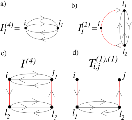
Figure 1: Lowest order diagram of a) $I^{(4)}$, b) $I^{(2)}$ and examples for long-range diagrams in c) $I^{(4)}$ and d) $T_{{\bf i},{\bf j}}^{(1),(1)}$.

To carry out the minimisation, as described in the previous section, we need to calculate the diagrams (30) and their derivatives with respect to lines up to a certain order in $x$. For example, the first-order diagram $I^{(4)}_{1}$ of $I^{(4)}$ is shown in Fig. 1a). Here, the lines can be normal ($P^{\sigma}_{{\bf i},{\bf l}_{1}}$) or anomalous ($S_{{\bf i},{\bf l}_{1}}$). With four normal lines, e.g., we have to evaluate

$$I^{(4)}_{1} = \sum_{{\bf l}_{1}(\neq{\bf i})}P^{\uparrow}_{{\bf i},{\bf l}_{1}}P^{\uparrow}_{{\bf l}_{1},{\bf i}}P^{\downarrow}_{{\bf i},{\bf l}_{1}}P^{\downarrow}_{{\bf l}_{1},{\bf i}}$$ (43)

$$= \frac{1}{L^{3}}\sum_{{\bf k},{\bf k}^{\prime},{\bf k}^{\prime\prime}}n_{{\bf k},\uparrow}n_{{\bf k}^{\prime},\uparrow}n_{{\bf k}^{\prime\prime},\downarrow}n_{{\bf k}+{\bf k}^{\prime}+{\bf k}^{\prime\prime},\downarrow}-n_{0}^{4}$$ (44)

where we have introduced the momentum-space distribution $n_{{\bf k},\sigma}\equiv\langle\hat{c}^{\dagger}_{{\bf k},\sigma}\hat{c}_{{\bf k},\sigma}\rangle_{0}$. Obviously, the real space evaluation of the diagram is numerically much easier because only one summation (over ${\bf l}_{1}$) has to be carried out. Moreover, the lines $P_{{\bf i},{\bf j}}$ in real space vanish like $1/\sqrt{|{\bf i}-{\bf j}|}$ while the number of neighbours of this distance is $\sim|{\bf i}-{\bf j}|$. Hence, the real-space contributions of $I^{(4)}_{1}$ fall off rapidly and we can restrict the summation over $l_{1}$ to a limited number of nearest neighbours of ${\bf i}$. This ‘locality’ of diagrams in real space is a key ingredient in our numerical implementation since it allows us to calculate diagrams up to relatively large orders in $x$.

Unfortunately, not all diagrams are as local as $I^{(4)}_{1}$. In particular, all diagrams in $I^{(2)}$, contain ‘long-range contributions’, e.g., the joint sum over ${\bf l}_{1}$, ${\bf l}_{2}$ in Fig. 1b). In the paramagnetic case, there exists a relationship between $I^{(2)}$ and $I^{(4)}$ which can be used to circumvent the long-range contributions in $I^{(2)}$, see Ref. [14]. No such relationship, however, can be used for superconducting states. Moreover, even for paramagnetic states some diagrams have long-range contributions, e.g., the $I^{(4)}$ and $T_{{\bf i},{\bf j}}^{(1),(1)}$ diagrams shown in Fig. 1. We may identify the diagrams with long-range contributions by a topological analysis, as we shall explain in the following Section 3. The real-space summations which belong to such long-range diagrams can then be evaluated analytically, see below.

3 Long-range diagrams

As explained in Section 2.2, some diagrams are not localised and require a special treatment in our real-space evaluation. Topologically, there are two types of diagrams which we need to consider up to the 4-th order (of internal vertices) in $x$. They are displayed in Figs. 2.

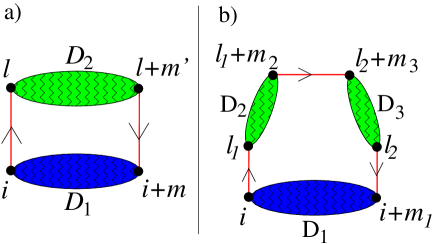
Figure 2: Long-range diagrams of a) type I, b) type II.

Diagrams of type I can be split into two disconnected diagrams $D_{1}$ and $D_{2}$ by cutting two lines, where the external vertices (${\bf i},{\bf j}$) belong to $D_{1}$. Examples for such diagrams are shown in Figs. 1b)-d). In a similar way we define diagrams of type II as those which can be split into three disconnected diagrams by cutting three (single) lines. An example for this type is the $I^{(2)}$ diagram shown in Fig. 3. It illustrates that type II diagram can only appear if there are at least four internal vertices. Note that more complicated long-range diagrams require the inclusion of more than five internal vertices.

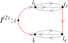
Figure 3: A type II diagram in $I^{(2)}$.

For the evaluation of the long-range diagrams in Figs. 2, one can carry out the sums over ${\bf l}$ (type I) or ${\bf l}_{1},{\bf l}_{2}$ (type II) analytically. We will consider the paramagnetic and the superconducting case separately in the following two sections.

3.1 The paramagnetic case

For the evaluation of the diagram in Fig. 2a), we need to calculate

$$D_{I}=\sum_{{\bf m},{\bf m}^{\prime}}D^{1}_{{\bf m},{\bf 0}}D^{2}_{{\bf 0},{\bf m}^{\prime}}\sum_{{\bf l}}\bar{P}^{\sigma}_{{\bf 0},{\bf l}}\bar{P}^{\sigma}_{{\bf l}+{\bf m}^{\prime},{\bf m}}$$ (45)

where $D^{1}$, $D^{2}$ are assumed to be localised diagrams, i.e., the sums over ${\bf m},{\bf m}^{\prime}$ can be restricted to a shell around ${\bf 0}$. The sum over ${\bf l}$ yields

$$\bar{D}({\bf m},{\bf m}^{\prime})\equiv\sum_{{\bf l}}\bar{P}^{\sigma}_{{\bf 0},{\bf l}}\bar{P}^{\sigma}_{{\bf l}+{\bf m}^{\prime},{\bf m}}$$

$$=\sum_{{\bf l}}(P^{\sigma}_{{\bf i},{\bf l}}-\delta_{{\bf i},{\bf l}}n_{0})(P^{\sigma}_{{\bf l}+{\bf m}^{\prime},{\bf i}+{\bf m}}-\delta_{{\bf l}+{\bf m}^{\prime},{\bf i}+{\bf m}}n_{0})$$

$$=(1-2n_{0})P^{\sigma}_{{\bf m},{\bf m}^{\prime}}+\delta_{{\bf m},{\bf m}^{\prime}}n_{0}^{2}\;.$$ (46)

Here we have used

$$\sum_{{\bf l}}P^{\sigma}_{{\bf i},{\bf l}}P^{\sigma}_{{\bf l}+{\bf m}^{\prime},{\bf i}+{\bf m}}=P^{\sigma}_{{\bf m},{\bf m}^{\prime}}\;,$$ (47)

which holds because, after Fourier transformation, in the paramagnetic case we can use $n_{{\bf k},\sigma}^{2}=n_{{\bf k},\sigma}$ in momentum-space. A long range-diagram of type I is therefore given as

$$D_{I}=\sum_{{\bf m},{\bf m}^{\prime}}D^{1}_{{\bf m},{\bf 0}}D^{2}_{{\bf 0},{\bf m}^{\prime}}\bar{D}({\bf m},{\bf m}^{\prime})\;.$$ (48)

Note that the diagram $D^{1}$ may contain additional long-range elements as, e.g., in the $I^{(2)}$ diagram in Fig. 4. In such a case, Eqs. (46)-(48) have to be applied consecutively.

In a long-range diagram of type II we need to evaluate

$$D_{II}=\sum_{{\bf m}_{1},{\bf m}_{2},{\bf m}_{3}}D^{1}_{{\bf m}_{1},{\bf 0}}D^{2}_{{\bf 0},{\bf m}_{2}}D^{3}_{{\bf m}_{3},{\bf 0}}\bar{D}({\bf m}_{1},{\bf m}_{2},{\bf m}_{3})$$ (49)

where

$$\bar{D}({\bf m}_{1},{\bf m}_{2},{\bf m}_{3})\equiv\sum_{{\bf l}_{1},{\bf l}_{2}}\bar{P}^{\sigma}_{{\bf 0},{\bf l}_{1}}\bar{P^{\sigma}}_{{\bf l}_{1}+{\bf m}_{2},{\bf l}_{2}+{\bf m}_{3}}\bar{P}^{\sigma}_{{\bf l}_{2},{\bf m}_{1}}\;,$$ (50)

The sums over ${\bf l}_{1}$, ${\bf l}_{2}$ can again be calculated exactly. This leads to

$$\bar{D}({\bf m}_{1},{\bf m}_{2},{\bf m}_{3}) = (1-3n_{0}+3n_{0}^{2})P^{\sigma}_{m_{2},m_{1}+m_{3}}$$ (51)

$$-\delta_{m_{2},m_{1}+m_{3}}n_{0}^{3}\;.$$

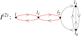
Figure 4: A type I diagram in $I^{(2)}$.

3.2 The superconducting case

In the superconducting case, the single (red) lines in Figs. 2 can be normal or anomalous. We therefore introduce the abbreviations

$$X^{1}_{{\bf i},{\bf j}} \equiv P^{\sigma}_{{\bf i},{\bf j}}\;,$$ (52)

$$X^{2}_{{\bf i},{\bf j}} \equiv S_{{\bf i},{\bf j}}\;,$$ (53)

$$\bar{X}^{\alpha}_{{\bf i},{\bf j}} \equiv X^{\alpha}_{{\bf i},{\bf j}}-\delta_{{\bf i},{\bf j}}X^{\alpha}_{{\bf 0},{\bf 0}}\;,$$ (54)

and the corresponding Fourier transforms

$$X^{1}_{{\bf k}} \equiv n_{{\bf k},\sigma}\;,$$ (55)

$$X^{2}_{{\bf k}} \equiv \langle\hat{c}_{{\bf k},\uparrow}\hat{c}_{-{\bf k},\downarrow}\rangle_{0}\;.$$ (56)

For long-range diagrams of type I we then have to evaluate

$$D^{\alpha,\alpha^{\prime}}_{I} = \sum_{{\bf m},{\bf m}^{\prime}}D^{1}_{{\bf m},{\bf 0}}D^{2}_{{\bf 0},{\bf m}^{\prime}}\bar{D}^{\alpha,\alpha^{\prime}}({\bf m},{\bf m}^{\prime})$$ (57)

$$\bar{D}^{\alpha,\alpha^{\prime}}({\bf m},{\bf m}^{\prime}) \equiv \sum_{{\bf l}}\bar{X}^{\alpha}_{{\bf 0},{\bf l}}\bar{X}^{\alpha^{\prime}}_{{\bf l}+{\bf m}^{\prime},{\bf m}}\;,$$ (58)

where $\alpha^{(\prime)}\in\{1,2\}$ characterises the two single lines in Fig. 2a). Note that $X^{2}_{{\bf 0},{\bf 0}}=0$ for our d-wave states. With a transformation to momentum space we find

$$\bar{D}^{\alpha,\alpha^{\prime}}({\bf m},{\bf m}^{\prime}) = Y^{\alpha,\alpha^{\prime}}_{{\bf m},{\bf m}^{\prime}}-X^{\alpha}_{{\bf 0},{\bf 0}}X^{\alpha^{\prime}}_{{\bf m},{\bf m}^{\prime}}-X^{\alpha^{\prime}}_{{\bf 0},{\bf 0}}X^{\alpha}_{{\bf m},{\bf m}^{\prime}}$$ (59)

$$+\delta_{{\bf m},{\bf m}^{\prime}}X^{\alpha}_{{\bf 0},{\bf 0}}X^{\alpha^{\prime}}_{{\bf 0},{\bf 0}}$$

with

$$Y^{\alpha,\alpha^{\prime}}_{{\bf m},{\bf m}^{\prime}}\equiv\frac{1}{L}\sum_{{\bf k}}X^{\alpha}_{{\bf k}}X^{\alpha^{\prime}}_{{\bf k}}e^{{\rm i}{\bf k}({\bf m}-{\bf m}^{\prime})}\;.$$ (60)

Note that, in the paramagnetic case, we have $Y^{1,1}_{{\bf m},{\bf m}^{\prime}}=P^{\sigma}_{{\bf m},{\bf m}^{\prime}}$, $X^{1}_{{\bf 0},{\bf 0}}=n_{0}$, such that Eq. (46) is recovered.

The evaluation of type II diagrams leads to

$$D^{\alpha_{1},\alpha_{2},\alpha_{3}}_{II} = \sum_{{\bf m}_{1},{\bf m}_{2},{\bf m}_{3}}D^{1}_{{\bf m}_{1},{\bf 0}}D^{2}_{{\bf 0},{\bf m}_{2}}D^{3}_{{\bf m}_{3},{\bf 0}}$$ (61)

$$\times\bar{D}^{\alpha_{1},\alpha_{2},\alpha_{3}}({\bf m}_{1},{\bf m}_{2},{\bf m}_{3})$$

where

$$\bar{D}^{\alpha_{1},\alpha_{2},\alpha_{3}}({\bf m}_{1},{\bf m}_{2},{\bf m}_{3})$$

$$\equiv\sum_{{\bf l}_{1},{\bf l}_{2}}\bar{X}^{\alpha_{1}}_{{\bf 0},{\bf l}_{1}}\bar{X}^{\alpha_{2}}_{{\bf l}_{1}+{\bf m}_{2},{\bf l}_{2}+{\bf m}_{3}}\bar{X}^{\alpha_{3}}_{{\bf l}_{2},{\bf m}_{1}}\;.$$ (62)

The momentum-space evaluation for (62) yields

$$\bar{D}^{\alpha_{1},\alpha_{2},\alpha_{3}}({\bf m}_{1},{\bf m}_{2},{\bf m}_{3})=Z^{\alpha_{1},\alpha_{2},\alpha_{3}}_{m_{2},m_{1}+m_{3}}$$

$$-[X^{\alpha_{1}}_{{\bf 0},{\bf 0}}Y^{\alpha_{2},\alpha_{2}}_{m_{2},m_{1}+m_{3}}+{\rm perm.}]$$

$$+[X^{\alpha_{1}}_{{\bf 0},{\bf 0}}X^{\alpha_{2}}_{{\bf 0},{\bf 0}}X^{\alpha_{3}}_{m_{2},m_{1}+m_{3}}+{\rm perm.}]$$

$$-\delta_{{\bf m}_{2},{\bf m}_{1}+{\bf m}_{3}}X^{\alpha_{1}}_{{\bf 0},{\bf 0}}X^{\alpha_{2}}_{{\bf 0},{\bf 0}}X^{\alpha_{3}}_{{\bf 0},{\bf 0}}$$ (63)

where ‘$+$perm.’ denotes the three cyclical permutations of $(\alpha_{1},\alpha_{2},\alpha_{3})$ in the respective functions and

$$Z^{\alpha_{1},\alpha_{2},\alpha_{3}}_{{\bf m},{\bf m}^{\prime}}\equiv\frac{1}{L}\sum_{{\bf k}}X^{\alpha_{1}}_{{\bf k}}X^{\alpha_{2}}_{{\bf k}}X^{\alpha_{3}}_{{\bf k}}e^{{\rm i}{\bf k}({\bf m}-{\bf m}^{\prime})}\;.$$ (64)

Note that in the superconducting case it is not possible to write the long-range contributions in terms of lines ($P^{\sigma}_{{\bf i},{\bf j}}$, $S_{{\bf i},{\bf j}}$) as it is possible in the paramagnetic case, see Eqs. (46) and (50). Instead, there appear the new objects $Y^{\alpha,\alpha^{\prime}}_{{\bf m},{\bf m}^{\prime}}$ and $Z^{\alpha_{1},\alpha_{2},\alpha_{3}}_{{\bf m},{\bf m}^{\prime}}$ whose calculation, however, is numerically benign because $|{\bf m}-{\bf m}^{\prime}|$ can be assumed to be small. Still, due to the appearance of these new objects, we need to reconsider the minimisation of our energy functional with respect to $|\Psi_{0}\rangle$. This problem is discussed in Appendix C.

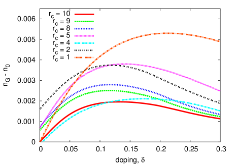
Figure 5: The $7$-th order Taylor expansion of (65) as a function of doping $\delta$ for $U/|t|=10$ and different values of the cutoff parameter $r_{\rm c}=1-10$ (calculated without LRDE).

4 Results

In our real-space evaluation of diagrams there are two main approximations that are needed to make the problem numerically treatable:

• The lines $\bar{P}^{\sigma}_{{\bf l},{\bf l}^{\prime}}$, $S_{{\bf l},{\bf l}^{\prime}}$ which enter the energy functional can have an arbitrary ‘length’

  $$|{\bf l}-{\bf l}^{\prime}|=\sqrt{(l_{1}-l^{\prime}_{1})^{2}+(l_{2}-l^{\prime}_{2})^{2}}\;.$$

  To keep the number of real-space contributions finite we need to introduce some ‘cutoff’ $r_{\rm c}$, i.e., the assumption that $\bar{P}^{\sigma}_{{\bf l},{\bf l}^{\prime}}=S_{{\bf l},{\bf l}^{\prime}}=0$ for $|{\bf l}-{\bf l}^{\prime}|^{2}>r_{\rm c}$. The cutoff leads to numerical errors in particular for the long-range diagrams discussed in Section 3. However, as we will demonstrate in the following section 4.1, these errors are negligible if we employ the long-range diagram evaluation (LRDE) technique introduced in Section 3.

• The number of diagrams grows exponentially with the number of internal vertices (index $k$ in Eqs. (31), (32)). Therefore, the diagrammatic expansion must be terminated at some finite value of $k$. As we will discuss in section 4.2, a better truncation parameter is the total number of lines in a diagram.

In all subsequent results, we have worked with a single-band Hamiltonian $\hat{H}_{0}$ that contains nearest and next-nearest neighbour hopping of $t=-0.35$eV and $t^{\prime}/t=-0.25$, respectively. These values are generally assumed to describe the situation in the Cuprates.

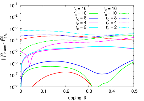
Figure 6: Difference between the exact value of the diagram $I^{(2)}_{1}$ (see Fig. 1b)) as a function of doping $\delta$ for several values of $r_{\rm c}$ with and without LRDE (solid and dashed lines, respectively).

4.1 Line cutoff

To analyse the role of a finite cutoff length $r_{\rm c}$ we first consider the expression for the correlated particle number per lattice site

$$n_{\rm G}-n_{0}=[1+xn_{0}(1-n_{0})]I^{(2)}+x(1-2n_{0})I^{(4)}$$ (65)

which results from Eqs. (12), (13), (2.1). The correlation operator $\hat{P}_{\rm G}$ in (4) commutes with the operator $\hat{N}\equiv\sum_{i,\sigma}\hat{n}_{i,\sigma}$ which counts the total number of electrons. Since, in the paramagnetic case, $|\Psi_{0}\rangle$ is an eigenstate of $\hat{N}$, we have $\langle\hat{N}\rangle_{\rm G}=\langle\hat{N}\rangle_{0}$ and therefore $n_{\rm G}-n_{0}=0$ in our translationally invariant system.

If we consider the r.h.s. of (65) as a power series in $x$ each coefficient of this expansion has to be exactly zero. Numerically, however, this is not the case because of our cutoff parameter $r_{\rm c}<\infty$. In Fig. 5, we plot the $7$-th order Taylor expansion of (65) as a function of doping for $U/|t|=10$ and different values of $r_{\rm c}$.

As we can see from this figure, an increase of $r_{\rm c}$ improves the results only slowly. Unfortunately, for higher-order diagrams it would not be feasible to work with values of $r_{\rm c}$ significantly larger than $10$. Therefore, the LRDE is essential to eliminate the error that stems from the finite cutoff $r_{\rm c}$. In fact, the LRDE ensures that the $7$-th order expansion in Fig. 5 is exactly zero for all cutoff parameters $r_{\rm c}$. This perfect agreement, however, is only due to the fact that the remaining errors in the calculation of $I^{(2)}$ and $I^{(4)}$ cancel each other exactly in (65). To gauge the remaining real-space cutoff error, we display in Fig. 6 the value of the diagram $I^{(2)}_{1}$ (see Fig. 1b)) relative to its exact value as a function of doping for several values of $r_{\rm c}$ with and without LRDE. Note that these values are independent of $x$ (cf. Eq. (31)) and only depend on the lines which we take from the ground state $|\Psi_{0}\rangle$ of the bare single particle Hamiltonian $\hat{H}_{0}$. Again, we can see from Fig. 6 that bringing down the numerical error by increasing $r_{\rm c}$ is not working well without the use of the LRDE: even for $r_{\rm c}=2$ (i.e., only nearest and next-nearest neighbour lines) the results with LRDE are more accurate than those for $r_{\rm c}=16$ and without LRDE.

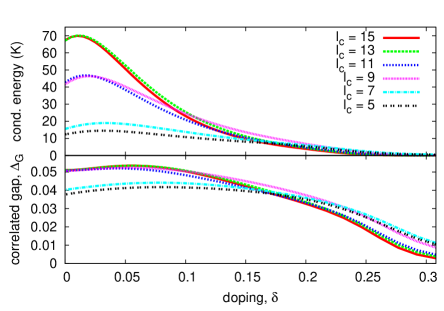
Figure 7: Condensation energy in Kelvin (upper panel) and correlated gap in the superconducting state (lower panel) as a function of doping $\delta$ for $U/|t|=10$ and different values of $l_{c}$.

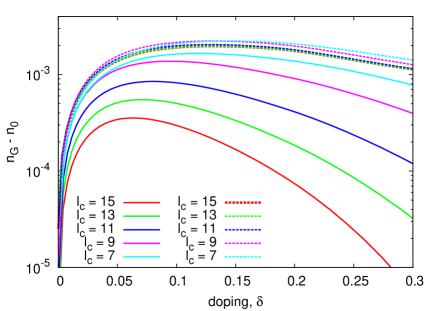
Figure 8: Difference $n_{\rm G}-n_{0}$ in the paramagnetic phase as a function of doping $\delta$ for $U/|t|=10$ and several values of $l_{c}$, with and without LRDE (solid and dashed lines, respectively).

4.2 Line number truncation

The natural expansion parameter appears to be the number $k$ of internal vertices in Eqs. (29)-(31). In fact, in our previous works on Pomeranchuk phases [14] and superconductivity [15] we have investigated the convergence of results as a function of the diagrammatic order $k$. However, the topological complexity of a diagram is more related to the number of lines in a diagram which is given as

$$N_{k} = 1+2k\;\;\;{\rm for}\;I^{(2)}[k],T^{(1)(1)}[k]\;,$$ (66)

$$N_{k} = 2+2k\;\;\;{\rm for}\;I^{(4)}[k],T^{(1)(3)}[k]\;,$$ (67)

$$N_{k} = 3+2k\;\;\;{\rm for}\;T^{(3)(3)}[k]\;.$$ (68)

As we have found already in a study on the $t$-$J$ model [18] it is more useful to include all diagrams up to a certain maximum number $l_{c}$ of lines. This means that in results with $l_{c}=15$ there are some diagrams included that have $k=7$ internal vertices. As an example for the convergence with respect to $l_{c}$, we show in Fig. 7 the condensation energy (energy difference between superconducting and paramagnetic ground state) and the ‘correlated gap’ $\Delta_{\rm G}\equiv\langle\hat{c}_{{\bf i},\uparrow}\hat{c}_{{\bf j},\downarrow}\rangle_{\rm G}$ (for nearest neighbours ${\bf i}$, ${\bf j}$) in the superconducting state for $U/|t|=10$ and as a function of doping for different values of $l_{c}$. All these data have been calculated using the LRDE (without LRDE we obtain qualitatively similar behavior, with the value of the condensation energy slightly increased, cf. also Fig. 9). As observed in previous studies, convergence of the condensation energy is reached for doping $\delta\gtrsim 0.1$. For smaller doping values the convergence is less satisfactory as compared to that of most other observables, e.g., the correlated gap. Figure 7 shows that the results for the latter have converged already for $l_{c}=11$. Since the condensation energy is largely increasing as a function of $l_{c}$, the stability of a superconducting state is very likely in the inaccessible limit $l_{c}\to\infty$. Note that the ground state energy of the paramagnetic phase (not plotted) is practically converged for $l_{c}=15$ (the differences in this energy between the results for $l_{c}=15$ and $l_{c}=11,13$ are below $1$K). Therefore, the error of the condensation energy comes mostly from the superconducting phase ground state energy. In the following analysis we work with $l_{c}=15$ and $r_{c}=10$, unless stated otherwise.

The importance of the LRDE is illustrated, once more, in Fig. 8 where we display $n_{\rm G}-n_{0}$ in the paramagnetic phase as a function of doping for $U/|t|=10$ and several values of $l_{c}$. The solid (dashed) lines show the results with (without) the LRDE. Obviously, the error that appears in the data without LRDE is so large, that there is hardly any improvement of the results if we increase $l_{c}$. In contrast, if we use the LRDE, $n_{\rm G}-n_{0}$ goes exponentially to zero if we increase $l_{c}$. Note that the remaining error stems from the fact, that contributions from the highest order in $x$ are not exactly cancelled as they were in the Taylor-series expansion discussed in the previous section 4.1.

In Fig. 9 we display the differences between energies that were calculated with and without the LRDE as a function of doping and for $U/|t|=10$. The differences shown in this figure are those for the kinetic, the potential and the total energy in the superconducting phase, as well as the condensation energy. As can be seen from this graph, the changes of the energies due to the LRDE are not negligible, in particular, for a doping of less than $0.1$. The total energy is lowered by up to $23$K if we use LRDE. The resulting change in the condensation energy, however, is smaller (less than $10$K). The same holds for other observables in the superconducting state. Therefore, the main results on superconductivity which we have published in our previous work [15] remain unchanged by the new LRDE scheme. However, the relatively large changes of the kinetic and the potential energy indicate that for other systems or states, the LRDE may alter physical properties more visibly.

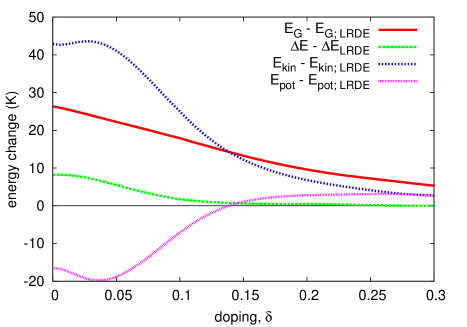
Figure 9: Differences between kinetic ($E_{\rm kin}$), potential ($E_{\rm pot}$), total ($E_{\rm G}$), and condensation ($\Delta E$) energy calculated with and without the LRDE as a function of doping $\delta$ and for $U/|t|=10$.

In Fig. 10 we show the difference between the kinetic energy of the paramagnetic and the superconducting phases. This property is negative for a conventional (BCS-type) superconductor, as pairing induces ’smearing’ of the single-particle distribution around the Fermi surface, which increases the kinetic part of the total energy. We observe such behaviour for $U\lesssim 12|t|$ at all doping values. For larger values of the Coulomb interaction ($U\gtrsim 13|t|$) the kinetic energy becomes lower in the superconducting phase. This is an unconventional behaviour coming from the fact that the bandstructure of the effective Hamiltonian changes upon condensation, which can dominate over the mentioned effect of an increased kinetic energy. The phenomenon of kinetic-energy driven superconductivity has also been observed experimentally for the cuprates [20, 21, 22, 23]. However, the experimental trend is different in the sense that there is a transition close to optimal doping from BCS-type behaviour (for large doping values) to kinetic-energy driven superconductivity (for small doping values). In our previous calculations [15] we obtained similar behaviour for $U\gtrsim 13|t|$, however the kinetic energy increase was always very small. The present results are more accurate and we observe that the kinetic energy change for overdoped systems is positive for $U\gtrsim 13|t|$. Close to the critical doping the kinetic energy change is very small (of the order of $1$K). It might be below the accuracy of our method to determine whether it is positive or negative in this regime (by changing $l_{c}$ we could observe both for $l_{c}=11,13,15$). The lack of transition between the two regimes in Gutzwiller Wave Function has been remedied in the variational Monte Carlo method [7, 8] by including in the projection also an additional Jastrow factor. This Jastrow factor is motivated by the form of a strong coupling expansion used to derive the $t$-$J$ model from the Hubbard model [24]. By including similar terms in the present method it should be possible to observe a behaviour consistent with the experimental data. Work along this line is planned in the future.

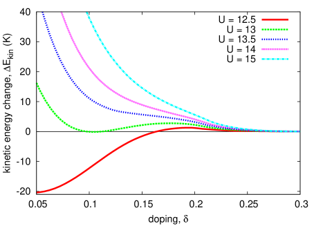
Figure 10: Kinetic energy change upon condensation $\Delta E_{\rm kin}$ as a function of doping $\delta$.

5 Summary and Outlook

In summary, we have given a comprehensive derivation of a diagrammatic variational method for the evaluation of superconducting states in two-dimensional Hubbard models. Since most diagrams in our scheme are rather localised in real space we are able to evaluate them up to relatively large orders in the expansion parameter $x$. For those diagrams which are not localised, we developed a resummation method that practically eliminates the numerical error in their real space evalution (e.g., we estimated this error to be of the order of $1$ K for the condensation energy). The remaining error of our method comes from the cutoff in the expansion in $x$. We have analyzed convergence of the condensation energy and correlated gap as a function of this cutoff. We have also studied the kinetic energy change upon condensation, a property that can be related to the experiment.

Our diagrammatic method is rather general and can be applied to various systems and situations. For the two-dimensional Hubbard model, it is still an open question whether a Pomeranchuk and a superconducting state are competing or coexisting near half filling. Also, the competition or coexistence of these two phases with antiferromagnetic order [25] has not yet been studied.

It is further possible to apply the method to more complicated model systems, in particular to those, in which methods based on the Gutzwiller Approximation have provided valuable insights, e.g., periodic Anderson models [26, 27], multi-layer Hubbard models, or multi-band Hubbard models [28, 29]. Work in all these directions is in progress. Also the study of non-local interactions and/or correlations [30] should be feasible in the future.

Appendix A Treatment of local pairing

In this Appendix, we explain how our diagrammatic formalism can be applied if the local pairing condition (8) is not fulfilled (e.g. for superconducting phase with $s$-wave symmetry component).

The basic idea remains the same as before, i.e, we aim to write $\hat{P}_{{\bf l}}^{\dagger}\hat{P}_{{\bf l}}$ in the form (9) with an operator $\hat{d}^{\rm HF}_{{\bf l}}$ that ensures the vanishing of all Hartree bubbles at internal vertices. Now, however, we need to cancel normal as well as anomalous Hartree bubbles. This requires the use of the more general local correlation operator

$$\hat{P}_{{\bf i}}=\sum_{\Gamma}\lambda_{\Gamma}|\Gamma\rangle_{{\bf i}\,{\bf i}}\!\langle\Gamma|+\lambda_{B}(|d\rangle_{{\bf i}\,{\bf i}}\!\langle\emptyset|+{\rm h.c.})\;.$$ (69)

Here we have already assumed that

$$\Delta_{0}\equiv\langle\hat{\Delta}_{{\bf l}}\rangle_{0}\;\;\;\;({\rm with}\;\;\hat{\Delta}_{{\bf l}}\equiv\hat{c}_{{\bf l},\downarrow}\hat{c}_{{\bf l},\uparrow})$$ (70)

is real which allows us to also work with a real parameter $\lambda_{B}$. The following considerations can be readily generalised in the case of a complex amplitude $\Delta_{0}$.

It will be useful to generalise the Hartree Fock operators (11). Let

$$\hat{O}_{{\bf l}}=\hat{\alpha}_{{\bf l},1}\dots\hat{\alpha}_{{\bf l},n}$$ (71)

be an arbitrary operator on site ${\bf l}$ where $\hat{\alpha}_{{\bf l},i}$ may be creation or annihilation operators. Then, we want

$$\hat{O}_{{\bf l}}^{\rm HF}=\hat{O}_{{\bf l}}-[\hat{O}_{{\bf l}}]^{\rm HF}$$ (72)

to create the same diagrams as $\hat{O}_{{\bf l}}$ apart from those with Hartree bubbles at site ${\bf l}$. This is achieved if we define $[\hat{O}_{{\bf l}}]^{\rm HF}$ recursively as

$$\left[\hat{\alpha}_{{\bf l},1}\ldots\hat{\alpha}_{{\bf l},n}\right]^{\rm HF}\equiv\left\langle\hat{\alpha}_{{\bf l},1}\ldots\hat{\alpha}_{{\bf l},n}\right\rangle_{0}$$

$$+ \mathop{{\sum}^{\prime}}_{\{\gamma_{1},...,\gamma_{n}\}=0}^{1}(-1)^{f_{\rm s}(\{\gamma_{i}\})}\left\{\left(\prod_{\ell=1}^{n}\hat{\alpha}_{{\bf l},\ell}^{\gamma_{\ell}}\right)-\left[\prod_{\ell=1}^{n}\hat{\alpha}_{{\bf l},\ell}^{\gamma_{\ell}}\right]^{\rm HF}\right\}$$

$$\times\left\langle\prod_{\ell=1}^{n}\hat{\alpha}_{{\bf l},\ell}^{1-\gamma_{\ell}}\right\rangle_{0}$$

with

$$f_{\rm s}(\{\gamma_{i}\})\equiv\sum_{\ell=1}^{n}\left(\ell-\frac{1}{2}\right)\gamma_{\ell}\;.$$ (74)

The prime in (A) indicates that

$$2\leq\sum_{\ell=1}^{n}\gamma_{\ell}\leq n-2$$ (75)

has to be even (odd) if $n$ is even (odd). Due to this summation restriction we find

$$\left[\hat{\alpha}_{{\bf l},i}\hat{\alpha}_{{\bf l},j}\right]^{\rm HF} = \langle\hat{\alpha}_{{\bf l},i}\hat{\alpha}_{{\bf l},j}\rangle_{0}\;,$$ (76)

$$\left[\hat{\alpha}_{{\bf l},i}\right]^{\rm HF} = 0\;.$$ (77)

Note that this recursive definition is quite general and covers systems with an arbitrary number of orbitals and local density matrices $\langle\hat{\alpha}_{{\bf i},i}\hat{\alpha}_{{\bf i},j}\rangle_{0}$. In the case of our single-band model with local pairing (70), we find, e.g.,

$$\hat{d}^{\rm HF}_{{\bf l}} = \hat{d}_{{\bf l}}-[\hat{c}_{{\bf l},\uparrow}^{\dagger}\hat{c}_{{\bf l},\uparrow}\hat{c}_{{\bf l},\downarrow}^{\dagger}\hat{c}_{{\bf l},\downarrow}]^{\rm HF}$$

$$= \hat{d}_{{\bf l}}-n_{0}(\hat{n}_{{\bf l},\uparrow}+\hat{n}_{{\bf l},\downarrow})-\Delta_{0}(\hat{\Delta}_{{\bf l}}+\hat{\Delta}^{\dagger}_{{\bf l}})+n^{2}_{0}+\Delta^{2}_{0}$$

for the Hartree Fock operator in Eq. (10). Another example which will be relevant for the evaluation of hopping expectation values is

$$[\hat{c}_{{\bf l},\uparrow}^{\dagger}\hat{c}_{{\bf l},\uparrow}\hat{c}_{{\bf l},\downarrow}]^{\rm HF}=n_{0}\hat{c}_{{\bf l},\downarrow}+\Delta_{0}\hat{c}_{{\bf l},\uparrow}^{\dagger}\;.$$ (79)

Together with (A), the operator equation (10). leads to

$$\lambda^{2}_{d}+\lambda^{2}_{B} = 1+(1-n_{0})^{2}x+\Delta^{2}_{0}x\;,$$ (80)

$$\lambda^{2}_{\sigma} = 1-n_{0}(1-n_{0})x+\Delta^{2}_{0}x\;,$$ (81)

$$\lambda^{2}_{\emptyset}+\lambda^{2}_{B} = 1+n_{0}^{2}x+\Delta^{2}_{0}x\;,$$ (82)

$$\lambda_{B}(\lambda_{d}+\lambda_{\emptyset}) = -x\Delta_{0}\;.$$ (83)

This set of equations determines, like in the case without local pairing, all parameters $\lambda_{\Gamma}$, $\lambda_{B}$ as a function of $x$.

To calculate the expectation value of a local doble occupancy, we use the relation

$$\hat{P}_{{\bf i}}^{\dagger}\hat{d}_{{\bf i}}\hat{P}_{{\bf i}} = (\lambda^{2}_{d}+\lambda^{2}_{B})\hat{d}^{\rm HF}_{{\bf i}}$$

$$+[(\lambda^{2}_{d}+\lambda^{2}_{B})n_{0}-\lambda^{2}_{B}](\hat{n}^{\rm HF}_{{\bf i},\uparrow}+\hat{n}^{\rm HF}_{{\bf i},\downarrow})$$

$$+[(\lambda^{2}_{d}+\lambda^{2}_{B})\Delta_{0}-\lambda_{B}\lambda_{d}](\hat{\Delta}^{\rm HF}_{{\bf i}}+{\rm h.c.})+\bar{d}_{0}$$

with

$$\hat{\Delta}^{\rm HF}_{{\bf i}}\equiv\hat{\Delta}_{{\bf i}}-\Delta_{0}$$ (85)

and

$$\bar{d}_{0}\equiv(\lambda^{2}_{d}+\lambda^{2}_{B})(n_{0}^{2}+\Delta_{0}^{2})+\lambda^{2}_{B}(1-2n_{0})+2\lambda_{B}\lambda_{d}\Delta_{0}\;.$$ (86)

This leads to

$$\langle\hat{d}_{{\bf i}}\rangle_{\rm G}=\bar{d}_{0}+2[(\lambda^{2}_{d}+\lambda^{2}_{B})n_{0}-\lambda^{2}_{B}]I^{(2)}$$ (87)

$$+(\lambda^{2}_{d}+\lambda^{2}_{B}-x\bar{d}_{0})I^{(4)}+2[(\lambda^{2}_{d}+\lambda^{2}_{B})\Delta_{0}-\lambda_{B}\lambda_{d}]I^{(2)}_{\rm s},$$

where we have introduced the (anomalous) diagrammatic sum

$$I^{(2)}_{\rm s}\equiv\sum_{k=0}^{\infty}\frac{x^{k}}{k!}\sum_{{\bf l}_{1},\ldots,{\bf l}_{k}}\bigl{\langle}\hat{\Delta}^{\rm HF}_{{\bf i}}\hat{d}^{\rm HF}_{{\bf l}_{1},\ldots,{\bf l}_{k}}\bigr{\rangle}^{\rm c}_{0}\;.$$ (88)

For the evaluation of a hopping expectation value we expand (19) , as in Eq. (24),

$$\widetilde{c}_{{\bf i},\sigma}^{\dagger} = q\hat{c}^{\dagger}_{{\bf i},\sigma}+\bar{q}\hat{c}_{{\bf i},\bar{\sigma}}+\alpha\Big{(}\hat{c}^{\dagger}_{{\bf i},\sigma}\hat{n}_{{\bf i},\bar{\sigma}}-[\hat{c}^{\dagger}_{{\bf i},\sigma}\hat{n}_{{\bf i},\bar{\sigma}}]^{\rm HF}\Big{)}$$ (89)

$$+\bar{\alpha}\Big{(}\hat{c}_{{\bf i},\bar{\sigma}}\hat{n}_{{\bf i},\sigma}-[\hat{c}_{{\bf i},\bar{\sigma}}\hat{n}_{{\bf i},\sigma}]^{\rm HF}\Big{)}$$

$$\widetilde{c}_{{\bf i},\sigma} = q\hat{c}_{{\bf i},\sigma}+\bar{q}\hat{c}^{\dagger}_{{\bf i},\bar{\sigma}}+\alpha\Big{(}\hat{c}_{{\bf i},\sigma}\hat{n}_{{\bf i},\bar{\sigma}}-[\hat{c}^{\dagger}_{{\bf i},\sigma}\hat{n}_{{\bf i},\bar{\sigma}}]^{\rm HF}\Big{)}$$ (90)

$$+\bar{\alpha}\Big{(}\hat{c}^{\dagger}_{{\bf i},\bar{\sigma}}\hat{n}_{{\bf i},\sigma}-[\hat{c}^{\dagger}_{{\bf i},\bar{\sigma}}\hat{n}_{{\bf i},\sigma}]^{\rm HF}\Big{)}$$

with

$$q \equiv \lambda_{1}[\lambda_{d}n_{0}+\lambda_{\emptyset}(1-n_{0})+2\lambda_{B}\Delta_{0}]\;,$$ (91)

$$\bar{q} \equiv \lambda_{1}[(\lambda_{d}-\lambda_{\emptyset})\Delta_{0}+\lambda_{B}(1-2n_{0})+2\lambda_{B}\Delta_{0}]\;,$$ (92)

$$\alpha \equiv \lambda_{1}(\lambda_{d}-\lambda_{\emptyset})\;,$$ (93)

$$\bar{\alpha} \equiv -2\lambda_{1}\lambda_{B}\;.$$ (94)

Using the above equations, it is now a straightforward task to write down the somewhat lengthy expressions for $\langle\hat{c}^{\dagger}_{{\bf i},\sigma}\hat{c}_{{\bf j},\sigma}\rangle_{\rm G}$ and $\langle\hat{c}^{\dagger}_{{\bf i},\uparrow}\hat{c}^{\dagger}_{{\bf j},\downarrow}\rangle_{\rm G}$.

Appendix B The linked-cluster theorem

In order to apply the linked-cluster theorem in (9) we need to lift the summation restrictions (20) in Eqs. (15)-(17). As we shall explain in this Appendix, the summation restriction can be lifted without generating additional terms.

We consider a diagram $D$ in which the two operators $\hat{c}_{{\bf l},\sigma}$ and $\hat{c}_{{\bf l}^{\prime},\sigma}$ from the two internal vertices ${\bf l}$, ${\bf l}^{\prime}$ have a contraction with two other operators $\hat{\alpha}_{1}$, $\hat{\alpha}_{2}$, respectively. The operators $\hat{\alpha_{i}}$ need not to be specified, i.e., they could be creation or annihilation operators and may belong to internal as well as external vertices. The diagram $D$ results as one term in the evaluation of

$$\langle\hat{c}_{{\bf l}^{\prime},\sigma}\hat{c}_{{\bf l},\sigma}\hat{\alpha}_{1},\hat{\alpha}_{2}\hat{O}_{\rm rest}\rangle_{0}$$ (95)

by means of Wicks theorem where $\hat{O}_{\rm rest}$ contains all other operators which appear in $D$. Hence, we can write $D$ as

$$D=\langle\hat{c}_{{\bf l},\sigma}\hat{\alpha}_{1}\rangle_{0}\langle\hat{c}_{{\bf l}^{\prime},\sigma}\hat{\alpha}_{2}\rangle_{0}D_{\rm rest}\;.$$ (96)

Another contribution from (95), however, is

$$D^{\prime}=-\langle\hat{c}_{{\bf l},\sigma}\hat{\alpha}_{2}\rangle_{0}\langle\hat{c}_{{\bf l}^{\prime},\sigma}\hat{\alpha}_{1}\rangle_{0}D_{\rm rest}\;.$$ (97)

If ${\bf l}={\bf l}^{\prime}$, we have $D+D^{\prime}=0$, i.e., both diagrams cancel each other. This explains why the summation restriction for the internal vertices can be lifted. The same arguments work if one of the two considered sites belongs to an external vertex, since all four operators $\hat{c}^{(\dagger)}_{{\bf l},\sigma}$ generate contractions for each internal vertex.

Note that after the application of the linked-cluster theorem, one must not reintroduce the summation restrictions. For instance, the diagram $D$ could be fully connected while in $D^{\prime}\equiv D^{\prime}_{\rm c}D^{\prime}_{\rm dc}$ the factor $D^{\prime}_{\rm dc}$ is cancelled by the norm. In such a case, the sum $D+D^{\prime}_{\rm dc}$ which results after the application of the linked-cluster theorem will, in general, not be zero even for ${\bf l}={\bf l}^{\prime}$.

Appendix C Minimisation with respect to $|\Psi_{0}\rangle$

C.1 Energy functional without long-range diagrams

If we ignore the non-locality of long-range diagrams, our Lagrange functional depends on $x$ and $|\Psi_{0}\rangle$ where $|\Psi_{0}\rangle$ enters the functional only via the elements of the single-particle density matrix

$$\tilde{\rho}^{\rm s}\equiv\left(\begin{array}[]{cc}\tilde{\rho}&\tilde{\Delta}\\ \tilde{\Delta}^{\dagger}&1-\tilde{\rho}\end{array}\right)\;.$$ (98)

Here we introduced

$$\rho_{({\bf i}\sigma),({\bf j}\sigma)} \equiv \langle\hat{c}_{{\bf j}\sigma}^{\dagger}\hat{c}_{{\bf j}\sigma}\rangle_{0}$$ (99)

$$\Delta_{({\bf i}\sigma),({\bf j}\bar{\sigma})} \equiv \langle\hat{c}_{{\bf j}\bar{\sigma}}\hat{c}_{{\bf j}\sigma}\rangle_{0}\;.$$ (100)

Since $\tilde{\rho}^{\rm s}$ is derived from a single-particle product state it has to obey the constraint $\tilde{\rho}^{\rm s}\cdot\tilde{\rho}^{\rm s}=\tilde{\rho}^{\rm s}$ . Like in the paramagnetic case we implement this constraint in the minimisation with respect to $\tilde{\rho}^{\rm s}$ by means of Lagrange parameters, see Refs. [31, 32]. This leads to the self-consistent single-particle problem introduced in Eqs. (7), (37)-(40)

C.2 Energy functional with long-range diagrams

When we evaluate the long-range diagrams as described in Section 3, we obtain an energy functional that does not only depend on the elements of $\tilde{\rho}^{\rm s}$ in real space, i.e., the lines $X^{\alpha}_{{\bf i},{\bf j}}$. It also depends on the ‘higher-order’ lines $Y^{\alpha,\alpha^{\prime}}_{{\bf i},{\bf j}}$ and $Z^{\alpha_{1},\alpha_{2},\alpha_{3}}_{{\bf i},{\bf j}}$ which, on the other hand, are determined by the elements of $\tilde{\rho}^{\rm s}$ in momentum space, i.e., the distributions $X_{{\bf k}}^{\alpha}$. Therefore, the great canonical potential has the form

$$\mathcal{F}(\{P_{{\bf i},{\bf j}}\},\{S_{{\bf i},{\bf j}}\};\{X_{{\bf k}}^{\alpha}\})$$ (101)

$$\equiv\mathcal{\bar{F}}\big{(}\{P_{{\bf i},{\bf j}}\},\{S_{{\bf i},{\bf j}}\};$$

$$\;\;\;\;\;\;\;\;\;\{Y^{\alpha,\alpha^{\prime}}_{{\bf i},{\bf j}}[\{X_{{\bf k}}^{\alpha}\}]\},\{Z^{\alpha_{1},\alpha_{2},\alpha_{3}}_{{\bf i},{\bf j}}[\{X_{{\bf k}}^{\alpha}\}]\}\big{)}\;.$$

Note that the lines $P_{{\bf i},{\bf j}}$, $S_{{\bf i},{\bf j}}$ enter the functional also via the evaluation of long-range diagrams, see Eqs. (52), (53), (59), (63). The minimisation of $\mathcal{F}$ with respect to $P_{{\bf i},{\bf j}}$, $S_{{\bf i},{\bf j}}$, and $X_{{\bf k}}^{\alpha}$ leads to

$$\hat{H}_{0}^{\rm eff}|\Psi_{0}\rangle=E_{0}|\Psi_{0}\rangle$$ (102)

where

$$\hat{H}_{0}^{\rm eff} = \sum_{{\bf i},{\bf j},\sigma}t^{\rm eff}_{{\bf i},{\bf j}}\hat{c}_{{\bf i},\sigma}^{\dagger}\hat{c}_{{\bf j},\sigma}^{\phantom{\dagger}}+\sum_{{\bf i}\neq{\bf j}}\bigl{(}\Delta^{\rm eff}_{{\bf i},{\bf j}}\hat{c}_{{\bf i},\uparrow}^{\dagger}\hat{c}_{{\bf j},\downarrow}^{\dagger}+{\rm h.c.}\bigr{)}$$ (104)

$$+\sum_{{\bf k},\sigma}\epsilon_{{\bf k}}\hat{n}_{{\bf k},\sigma}+\left(\sum_{{\bf k}}\Delta_{{\bf k}}\hat{c}^{\dagger}_{{\bf k},\uparrow}\hat{c}^{\dagger}_{-{\bf k},\downarrow}+{\rm h.c.}\right)$$

and

$$t^{\rm eff}_{{\bf i},{\bf j}} = \frac{\partial\mathcal{F}}{\partial P_{{\bf i},{\bf j}}}\;,\quad\Delta^{\rm eff}_{{\bf i},{\bf j}}=\frac{\partial\mathcal{F}}{\partial S_{{\bf i},{\bf j}}}\;,$$ (105)

$$\epsilon_{{\bf k}} = \frac{\partial\mathcal{F}}{\partial X^{1}_{{\bf k}}}\;,\quad\Delta_{{\bf k}}=\frac{\partial\mathcal{F}}{\partial X^{2}_{{\bf k}}}\;.$$ (106)

Equation (101) then yields

$$\epsilon_{{\bf k}} = \sum_{\alpha}(r^{1,\alpha}_{{\bf k}}+r^{\alpha,1}_{{\bf k}})X^{\alpha}_{{\bf k}}$$

$$+\sum_{\alpha,\alpha^{\prime}}(v^{1,\alpha,\alpha^{\prime}}_{{\bf k}}+v^{\alpha,1,\alpha^{\prime}}_{{\bf k}}+v^{\alpha,\alpha^{\prime},1}_{{\bf k}})X^{\alpha}_{{\bf k}}X^{\alpha^{\prime}}_{{\bf k}}\;,$$

$$\Delta_{{\bf k}} = \sum_{\alpha}(r^{2,\alpha}_{{\bf k}}+r^{\alpha,2}_{{\bf k}})X^{\alpha}_{{\bf k}}$$

$$+\sum_{\alpha,\alpha^{\prime}}(v^{2,\alpha,\alpha^{\prime}}_{{\bf k}}+v^{\alpha,2,\alpha^{\prime}}_{{\bf k}}+v^{\alpha,\alpha^{\prime},2}_{{\bf k}})X^{\alpha}_{{\bf k}}X^{\alpha^{\prime}}_{{\bf k}}\;.$$

where

$$r^{\alpha,\alpha^{\prime}}_{{\bf k}} \equiv \frac{1}{L}\sum_{{\bf i},{\bf j}}e^{{\rm i}{\bf k}({\bf j}-{\bf i})}\frac{\partial}{\partial Y_{{{\bf i},{\bf j}}}^{\alpha,\alpha^{\prime}}}\bar{\mathcal{F}}\;,$$ (109)

$$v^{\alpha_{1},\alpha_{2},\alpha_{3}}_{{\bf k}} \equiv \frac{1}{L}\sum_{{\bf i},{\bf j}}e^{{\rm i}{\bf k}({\bf j}-{\bf i})}\frac{\partial}{\partial Z_{{{\bf i},{\bf j}}}^{\alpha_{1},\alpha_{2},\alpha_{3}}}\bar{\mathcal{F}}\;.$$ (110)

References

- [1] J. Bardeen, L. N. Cooper, and J. R. Schrieffer, Phys. Rev. 108, 1175 (1957).
- [2] E. Feenberg, Theory of Quantum Liquids (Academic Press, New York, 1969).
- [3] B. E. Clements, E. Krotscheck, J. A. Smith, and C. E. Campbell, Phys. Rev. B 47, 5239 (1993).
- [4] M. Gutzwiller, Phys. Rev. Lett 10, 159 (1963).
- [5] M. Gutzwiller, Phys. Rev. 134, A923 (1964).
- [6] M. Gutzwiller, Phys. Rev. 137, A1726 (1965).
- [7] H. Yokoyama, Y. Tanaka, M. Ogata, and H. Tsuchiura, J. Phys. Soc. Jpn. 73, 1119 (2004).
- [8] H. Yokoyama, M. Ogata, Y. Tanaka, K. Kobayashi, and H. Tsuchiura, J. Phys. Soc. Jpn. 82, 014707 (2013).
- [9] D. Baeriswyl, Found. Phys. 30, 2033 (2000).
- [10] B. Hetényi, Phys. Rev. B 82, 115104 (2010).
- [11] P. Horsch and T. A. Kaplan, J. Phys. C: Solid State Phys. 16, L1203 (1983).
- [12] E. Koch, O. Gunnarsson, and R. M. Martin, Phys. Rev. B 59, 15632 (1999).
- [13] B. Edegger, C. Gros, and V. N. Muthukumar, Adv. Phys. 56, 927 (2007).
- [14] J. Büneman, T. Schickling, and F. Gebhard, Europhys. Lett. 98, 27006 (2012).
- [15] J. Kaczmarczyk, J. Spałek, T. Schickling, and J. Bünemann, Phys. Rev. B 88, 115127 (2013).
- [16] J. Kaczmarczyk, J. Bünemann, and J. Spałek, New J. Phys. 16, 073018 (2014).
- [17] J. Bünemann, S. Wasner, E. v. Oelsen, and G. Seibold, Philosophical Magazine (2014).
- [18] J. Kaczmarczyk, Philosophical Magazine (2014).
- [19] A. L. Fetter and J. D. Walecka, Quantum Theory of Many-Particle Systems (Dover Publications, New York, 2003).
- [20] G. Deutscher, A. F. Santander-Syro, and N. Bontemps, Phys. Rev. B 72, 092504 (2005).
- [21] N. Gedik, M. Langner, J. Orenstein, S. Ono, Y. Abe, and Y. Ando, Phys. Rev. Lett. 95, 117005 (2005).
- [22] C. Giannetti, F. Cilento, S. D. Conte, G. Coslovich, G. Ferrini, H. Molegraaf, M. Raichle, R. Liang, H. Eisaki, M. Greven, A. Damascelli, D. van der Marel, and F. Parmigiani, Nat. Commun. 2, 353 (2011).
- [23] F. Carbone, A. B. Kuzmenko, H. J. A. Molegraaf, E. van Heumen, V. Lukovac, F. Marsiglio, D. van der Marel, K. Haule, G. Kotliar, H. Berger, S. Courjault, P. H. Kes, and M. Li, Phys. Rev. B 74, 064510 (2006).
- [24] J. Spałek, Acta Physica Polonica A 111, 409 (2007).
- [25] J. Kaczmarczyk and J. Spałek, Phys. Rev. B 84, 125140 (2011).
- [26] O. Howczak, J. Kaczmarczyk, and J. Spałek, Phys. Status Solidi B 250(3), 609 (2013).
- [27] M. M. Wysokiński, M. Abram, and J. Spałek, Phys. Rev. B 90, 081114(R) (2014).
- [28] J. Bünemann, W. Weber, and F. Gebhard, Phys. Rev. B 57, 6896 (1998).
- [29] M. Zegrodnik, J. Bünemann, and J. Spałek, New J. Phys. 16(3), 033001 (2014).
- [30] M. Abram, J. Kaczmarczyk, J. Jȩdrak, and J. Spałek, Phys. Rev. B 88, 094502 (2013).
- [31] G. Seibold, F. Becca, and J. Lorenzana, Phys. Rev. B 78, 045114 (2008).
- [32] J. Bünemann, F. Gebhard, T. Schickling, and W. Weber, Phys. Status Solidi B 249, 1282 (2012).