X-ray emission from stellar jets by collision against high-density molecular clouds: an application to HH 248

Abstract

We investigate the plausibility of detecting X-ray emission from a stellar jet that impacts against a dense molecular cloud. This scenario may be usual for classical T Tauri stars with jets in dense star-forming complexes. We first model the impact of a jet against a dense cloud by 2D axisymmetric hydrodynamic simulations, exploring different configurations of the ambient environment. Then, we compare our results with XMM-Newton observations of the Herbig-Haro object HH 248, where extended X-ray emission aligned with the optical knots is detected at the edge of the nearby IC 434 cloud. Our simulations show that a jet can produce plasma with temperatures up to $10^{7}$ K, consistent with production of X-ray emission, after impacting a dense cloud. We find that jets denser than the ambient medium but less dense than the cloud produce detectable X-ray emission only at the impact onto the cloud. From the exploration of the model parameter space, we constrain the physical conditions (jet density and velocity, cloud density) that reproduce well the intrinsic luminosity and emission measure of the X-ray source possibly associated with HH 248. Thus, we suggest that the extended X-ray source close to HH 248 corresponds to the jet impacting on a dense cloud.

1 Introduction

Classical T Tauri stars (CTTSs) are characterized by being surrounded by a disk of gas as a result of the conservation of angular momentum during the star-formation process. The central star accretes material from the disk through magnetic funnels (Koenigl, 1991). In addition, dense gas from the inner region of the disk is collimated into a jet as explained in the context of the widely accepted theory of magneto-centrifugal launching (Ferreira et al., 2006). Recently, magneto-hydrodynamic (MHD) simulations have been performed to evaluate the importance of the accretion disk magnetic field in the launching process of a stellar jet (Matsakos et al., 2008, 2009; Stute et al., 2014; Staff et al., 2014). The role of the magnetic field for the collimation of stellar jets in laboratory plasma experiments has been recently explored by Albertazzi et al. (2014) through detailed numerical simulations and comparison with observations.

When escaping from the stellar system, the jet moves through circumstellar and interstellar material, interacting with the ambient medium and producing shocks. Usually, stellar jets are revealed in the optical by the presence of a chain of knots, the so-called Herbig-Haro (HH) objects. These knots are known to be associated with the jet’s shock front and post-shock regions. Supersonic shock fronts and post-shock regions along the jet are detected in a wide wavelength range, from radio to optical band (Reipurth & Bally, 2001, and references therein) and may be detected also in the ultraviolet (e.g. Gómez de Castro & von Rekowski, 2011; Coffey et al., 2012; Schneider et al., 2013). The knotty structure of HH objects within the jet axis is interpreted as the consequence of the pulsing nature of the ejection of material by the star (see Bonito et al., 2010a). A possible explanation for this pulsing nature is the variable nature of the stellar wind (Matsakos et al., 2009), whether through stellar magnetic cycles or by variations in the accretion rates.

Pravdo et al. (2001) observed high energy emission from high speed HH jets. In particular, hydrodynamic (HD) models predict X-ray emission from mechanical heating due to shocks produced by the interaction between the jet and the ambient medium (Bonito et al., 2004). This is particularly true when the jet is less dense than the ambient medium (Bonito et al., 2007). Instead, X-ray emission from heavy jets, i.e. jets that are denser than the ambient, is weaker. The analysis of X-ray data from stellar jets can yield constraints to initial conditions of the process such as the jet velocity and density. However, the low statistics in the few stellar jets detected in X-rays so far makes it difficult to achieve robust results (see Güdel et al., 2005, for an example).

X-ray emission from protostellar jets was firstly reported by Pravdo et al. (2001), who detected an X-ray source coincident with HH 2 that was not associated with any other galactic or extragalactic source (see Velusamy et al., 2014). Later, Favata et al. (2002) detected X-ray emission from HH 154, a jet associated with the protostar L1551 IRS5 in the Taurus Molecular Cloud (see also Bally et al., 2003; Bonito et al., 2004, 2011; Favata et al., 2006). Since then, the number of X-ray detections from protostellar jets has been increased: HH 80/81 (Pravdo et al., 2004), TKH 8 (Tsujimoto et al., 2004), HH 540 (Kastner et al., 2005), HH 210 (Grosso et al., 2006), HH 216 (Linsky et al., 2007), HH 168 (Pravdo et al., 2009).

Several jets from other young stellar objects (YSO) were detected in X-rays, too. Güdel et al. (2005) reported likely detection from a jet from the CTTS DG Tau (see Güdel et al., 2008; Schneider et al., 2013, for recent results). Skinner et al. (2011) detected evidence for extended X-ray structure in RY Tau. Finally, X-ray emission from a jet arising from the FU Ori type star Z CMa was detected by Stelzer et al. (2009). A list of X-ray detections and properties of stellar jets is given in Bonito et al. (2010b). The analysis of the X-ray spectrum of stellar jets divides them into two classes (Bonito et al., 2010b): (1) X-ray sources detected at the base of the jet (within 2000 AU from the stellar source), with temperature $>2\times 10^{6}$ K and (2) X-ray sources detected at large distances from the jet source (several thousands of AU), characterized by high luminosity and low temperature. The interpretation of this behavior is still not clear, but the difference between both classes seems to be related to the location of the X-ray emission.

In this work, we study a different scenario for X-ray emission observed from a jet: a stellar jet that moves through the interstellar medium (ISM) and impacts a molecular cloud (wall) with a density several times higher than that of the ambient. In this scenario, the jet is heavier than the ISM but lighter than the wall. We perform simulations with different initial conditions, widely exploring the parameter space. To test our results, we compared them with the jet HH 248, detected in X-rays with the XMM-Newton mission (Src. 12 in López-García et al., 2013).

The organization of this article is as follows. In Section 2, we present the numerical setup for our simulations. Results for the different initial conditions explored by us are discussed in Section 3. We then study the case of HH 248. A brief description of the system is carried out in Sections 4. Specific simulations for HH 248 are performed in Section 5. Final discussion and conclusions are presented in Section 6.

2 Hydrodynamic model and numerical setup

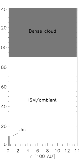
Figure 1: Schematic of the simulation domain setup. Boundary condition at the left border is reflective/axisymmetric. Outflow conditions are permitted in the remaining boundaries.

Our model describes the impact of a protostellar jet against a dense molecular cloud. We adopted the hydrodynamic model discussed by Bonito et al. (2007, hereafter BOP07), extended to include an ambient environment characterized by the presence of a dense cloud. The jet impact is modeled by numerically solving the time-dependent hydrodynamic equations of mass, momentum, and energy conservation in a 2D cylindrical coordinate system $(r,z)$, assuming axisymmetry (see BOP07 for details). The model includes the radiative losses from optically thin plasma, and the thermal conduction, including the effects of heat flux saturation. The model is implemented using the FLASH code (Fryxell et al., 2000), with the Piecewise Parabolic Method (PPM) solver that is better adapted for compressible flows with shocks (Colella & Woodward, 1984).

The jet is assumed to propagate along the symmetry axis, $z$, through an unperturbed ambient medium with a dense molecular cloud. The cloud is described by a higher density region (wall) in pressure equilibrium with its surrounding and is situated at $\sim 9000$ AU from the base of the domain (see Figure 1). We chose this distance as we want to compare the results from the simulations with the observations of HH 248 (see Section 5 for more details). The computational domain extends $\sim 1400$ AU in the $r$ direction and $\sim 14000$ AU in the $z$ direction. At the coarsest resolution, the adaptive mesh algorithm used in the FLASH code (PARAMESH; MacNeice et al., 2000) uniformly covers the 2D computational domain with an initial mesh of $1\times 10$ blocks, each with $8^{2}$ cells. We allow for five levels of refinement, with resolution increasing twice at each refinement level. The refinement criterion adopted (Löhner, 2008) follows the changes in density and temperature. This grid configuration yields an effective resolution of $\sim 7$ AU at the finest level, corresponding to an equivalent uniform mesh of $128\times 1280$ grid points.

We explore the parameter space defined by the density ratio between the ISM and the jet ($n_{\mathrm{ambient}}/n_{\mathrm{jet}}$), the density ratio between the wall and jet ($n_{\mathrm{wall}}/n_{\mathrm{jet}}$), and the jet’s velocity ($v_{\mathrm{jet}}$). The aim is to investigate which physical conditions result in the production of detectable X-rays from the stellar jet after impacting the dense cloud (preliminary results in Orellana et al., 2012). The grid of explored parameters is chosen in order to explore in detail the case of a jet over-dense in the ISM that becomes under-dense in the cloud. According to previous results (e.g. Bonito et al., 2007), this is the most promising scenario for X-ray emission. For completeness, we also explore the remaining two possible scenarios in less detail: the jet being heavier than both the ambient and the molecular cloud and the jet being lighter than both the ambient and the molecular cloud. The initial temperature of the jet is fixed to the value $T_{\mathrm{jet}}=10^{4}$ K in all the simulations. Figure 2 shows the parameter space for our simulation. The shaded area represents the region of the parameter space in which the ambient would be denser than the molecular cloud. This scenario is not explored in this work. In BOP07, it is shown that detectable X-ray emission originates from the interaction of light jets with the ambient medium. Here we explore the scenario of a jet heavier than the ambient but lighter than the molecular cloud. This scenario corresponds to the top-left quadrant in the figure. Table 1 summarizes the parameters of our simulations. The size of the circles in Figure 2 corresponds to four different velocity ranges for the jet: $v_{\mathrm{jet}}<500$ km s^-1, $500\leq v_{\mathrm{jet}}<1200$ km s^-1, $1200\leq v_{\mathrm{jet}}<2000$ km s^-1 and $v_{\mathrm{jet}}\geq 2000$ km s^-1, respectively from smaller to larger circles. In most cases, we simulated jets with different initial velocities for the same values of $n_{\mathrm{ambient}}/n_{\mathrm{jet}}$ and $n_{\mathrm{wall}}/n_{\mathrm{jet}}$.

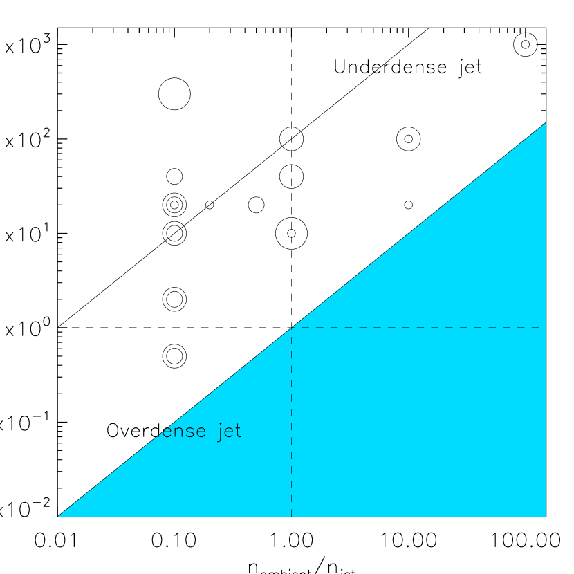
Figure 2: Parameter space of the simulations performed in this work. Small circles correspond to jet’s velocities $v_{\mathrm{jet}}\leq 500$ km s^-1, medium-size circles are for $500\leq v_{\mathrm{jet}}<1200$ km s^-1, and large circles are for simulations with $1200\leq v_{\mathrm{jet}}<2000$ km s^-1 and $v_{\mathrm{jet}}\geq 2000$ km s^-1, respectively. The shaded area is the scenario with a molecular cloud less dense than the ambient, which is not investigated in this article. The continuous line corresponds to $n_{\mathrm{wall}}/n_{\mathrm{ambient}}=100$.

Table 1: Summary of the simulations performed in this work.

$n_{\mathrm{ambient}}/n_{\mathrm{jet}}$	$n_{\mathrm{wall}}/n_{\mathrm{jet}}$	$Mach$	$v_{\mathrm{jet}}$	$\log T_{\mathrm{max}}$
			(km s-1)	(K)
0.1	0.5	20	936	6.70
”	0.5	30	1404	6.84
”	2.0	20	936	6.62
”	2.0	30	1404	6.80
”	10.0	20	936	6.57
”	10.0	30	1404	6.84
”	20.0	10	448	5.70
”	20.0	20	936	6.54
”	20.0	30	1404	6.83
”	40.0	20	936	6.64
”	300.0	150	2000	7.33
0.2	20.0	20	662	6.04
0.5	20.0	40	800	6.41
1.0	10.0	20	296	4.70
”	10.0	200	2960	7.18
”	40.0	100	1480	6.95
”	100.0	100	1480	7.08
10.0	20.0	100	448	5.10
”	100.0	100	448	5.60
”	100.0	300	1404	6.91
100.0	1000.0	100	148	4.40
-	1000.0	1000	1480	7.20

3 Results from simulations

The evolution of the density and temperature of a jet with distinct ambient-to-jet density ratios ($n_{\mathrm{ambient}}/n_{\mathrm{jet}}$) when traveling through a homogeneous ambient was investigated in detail in BOP07. In such work, it was shown that the case of a light jet ($n_{\mathrm{ambient}}/n_{\mathrm{jet}}>1$) with high Mach number ($M_{\mathrm{jet}}$) is the most favorable for detection of X-rays. A hot ($T>10^{6}$ K) and dense blob is formed behind the front shock in both light and heavy ($n_{\mathrm{ambient}}/n_{\mathrm{jet}}<1$) jets when the jet’s velocity is high enough, but in heavy jets this blob is fainter in X-rays and considerably less extended (see Figure 8 in BOP07). In fact, the shock velocity required to produce this faint X-ray emission in heavy jets is too high compared to observations ($v_{\mathrm{sh}}>2000$ km s^-1). At lower velocities, the X-ray luminosity of the heavy jet is low (see BOP07). Consequently, detection of X-ray emission from heavy jets is not expected. Instead, the jet’s luminosity increases rapidly when it becomes lighter than the ambient (see Section 5, Figure 7).

To illustrate the previous discussion, we compare the evolution of the mass density and temperature of a heavy jet with similar initial conditions but different velocities. Figure 3 shows mass density and velocity cuts in the r–z plane for jets with $M=10,20,30$ and $150$, respectively. In the four cases, the initial jet temperature is $10^{4}$ K and the ambient-to-jet density ratio is $n_{\mathrm{ambient}}/n_{\mathrm{jet}}=0.1$. The simulation was stopped at $d\sim 8500$ AU in each case, for purposes of comparison.

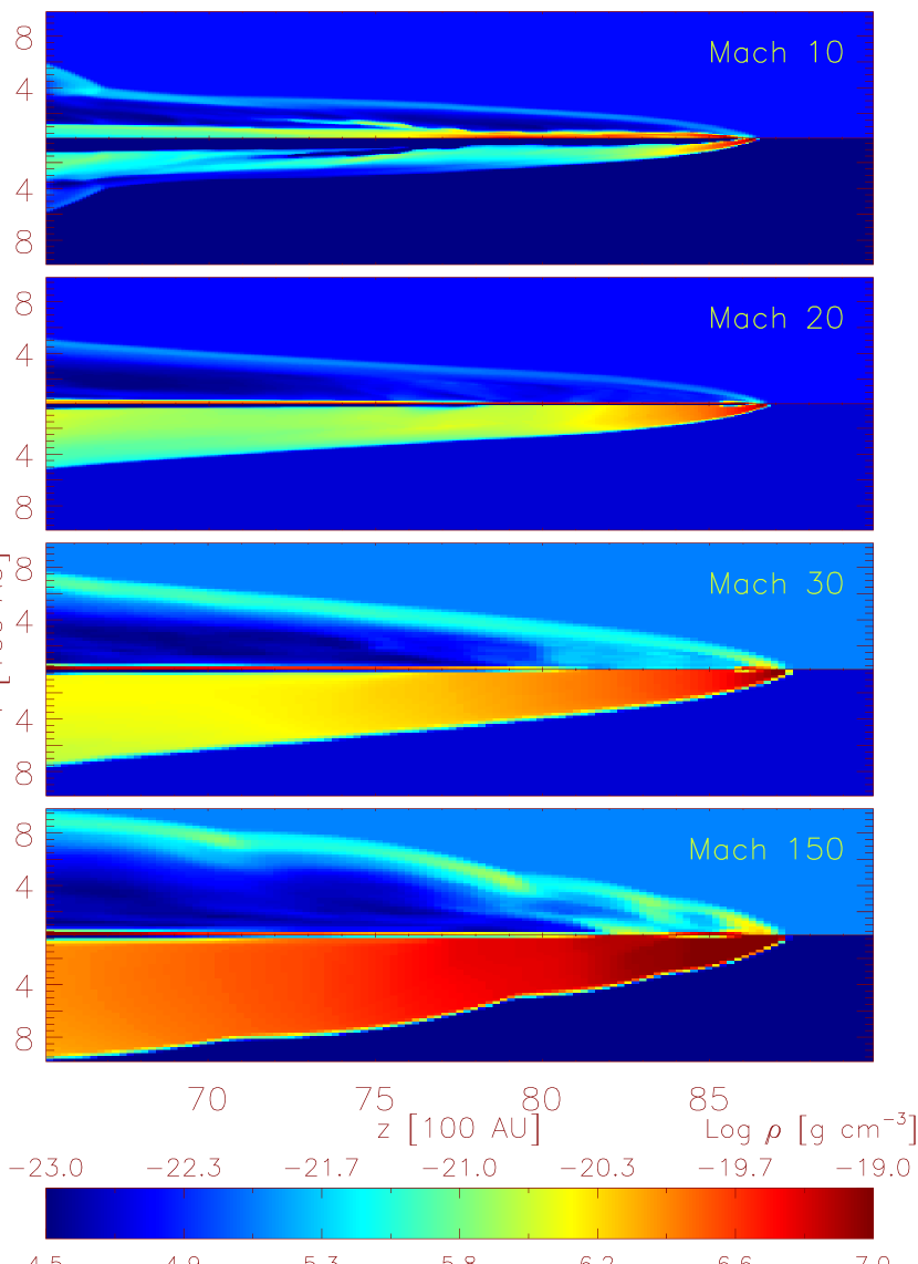
Figure 3: Two-dimensional mass density (upper half-panels) and temperature (lower half-panels) cuts in the r–z plane when the jet reaches 8000 AU from the beginning of the simulation. All the simulations are for $n_{\mathrm{ambient}}/n_{\mathrm{jet}}=0.1$ but different Mach numbers.

Last column in Table 1 shows the maximum temperature reached by the jet after impacting the dense cloud for each simulation. Temperatures similar to those observed in several X-ray emitting stellar jets (see Section 1) are reached when the velocity of the jet is of the order of 700 km s^-1 or higher.

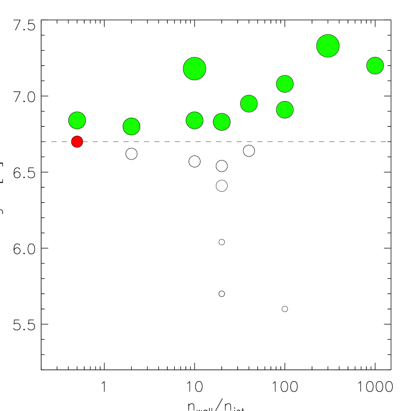
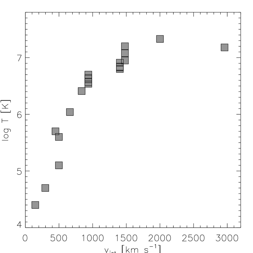
Figure 4: Top: Maximum temperature of the jet after impacting the dense cloud for the different simulations, compared to the ratio between the jet and the dense cloud densities. Circle sizes are as in Figure 2. The dashed line indicates a temperature of 5 MK ($kT=0.43$ keV). Filled circles are cases in which the jet reaches temperatures consistent with detected jets in X-rays. Bottom: Temperature distribution as a function of the velocity of the jet.

In Figure 4, we summarize the results of our simulations. The top figure represents the temperature reached when the jet comes into the dense cloud ($z\sim 120$ AU in Figure 1) as a function of the ratio between the density of the cloud and the jet. The bottom panel shows the maximum temperature as a function of the jet’s velocity. No clear dependence of the temperature with $n_{\mathrm{wall}}/n_{\mathrm{jet}}$ is observed (top panel). At high density ratios ($n_{\mathrm{wall}}/n_{\mathrm{jet}}>20$), there is only a slight trend of increasing the jet’s temperature with increasing the density ratio. Filled circles in this figure are simulations with $v_{\mathrm{jet}}\geq 700$ km s^-1. On contrast, Figure 4, bottom panel shows the temperature of the jet increases rapidly with increasing the jet’s velocity. Actually, the temperature reaches a plateau at $\sim 1200$ km s^-1 where it remains approximately constant ($\sim 10^{7}$ K) with increasing velocity. For $v_{\mathrm{jet}}\geq 700$ km s^-1, the jet reaches temperatures compatible with X-ray emission ($T\geq 10^{6}$ K).

Summarizing, a high jet’s velocity is responsible for the X-ray emission detected when the jet is lighter than the surrounding medium in the proposed scenario.

4 HH 248: a candidate for the jet-cloud impact scenario

The Herbig-Haro object HH 248 is situated to the South-East of the CTTS V615 Ori, at the base of the Horsehead Nebula (Barnard 33) and to the South of the NGC 2023 nebula (Malin et al., 1987). The detection of an X-ray source at $\sim 15\arcsec$ from HH 248 and $\sim 30\arcsec$ from V615 Ori ($05^{\mathrm{h}}$ $41^{\mathrm{m}}$ $25.7^{\mathrm{s}}$, $-02\arcdeg$ $23\arcmin$ $06.0\arcsec$) was reported by López-García et al. (2013) (their Src. 12). The authors did not find any optical or IR counterpart down to 0.1 mJy. Src. 12 of López-García et al. (2013) is classified as an extended source by the XMM-Newton SAS source detection task, discarding an association with any possible highly absorbed point-like source. The XMM-Newton observation (ID 0112640201, revolution 419) was centered on the reflection nebula NGC 2023. The extended X-ray source was detected $\sim 7\arcmin$ off-axis. Its proximity to the CTTS V615 Ori may be interpreted as they are related. However, an analysis of the spectrum of this X-ray source gives $N_{\mathrm{H}}=2.3_{-1.4}^{+2.6}\times 10^{22}$ cm^-3 (errors are at 90% confidence level) for the column density of the source and $T\sim 10^{7}$ K as a lower limit. The $N_{\mathrm{H}}$ value is considerably larger than the one obtained by López-García et al. (2013) for V615 Ori ($N_{\mathrm{H}}=0.50_{-0.04}^{+0.05}\times 10^{22}$ cm^-3). We conclude that V615 Ori is not the driving source of the extended X-ray emission detected.

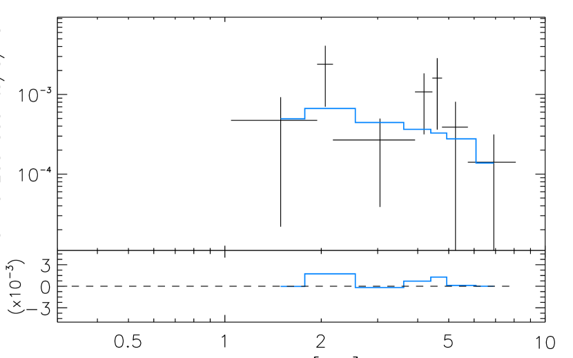
Figure 5: Background-subtracted XMM/EPIC spectrum of the extended source including the model fit.

Assuming a distance of $\sim 400$ pc for the source, $L_{\mathrm{X}}=3\pm 2\times 10^{30}$ erg s^-1 and $EM\approx 2\times 10^{53}$ cm^-3. This analysis was performed by ourselves by fitting an absorbed hot plasma model (Smith et al., 2001) to the observed EPIC/PN spectrum using the XSPEC spectral fitting package (Arnaud, 1996, 2004) with Cash statistics (Cash, 1979). We notice that XSPEC treats both the source and the background spectra separately when Cash statistics is used. The poor statistics of the source does not permit to study the properties of the X-ray emission in more detail (see Figure 5).

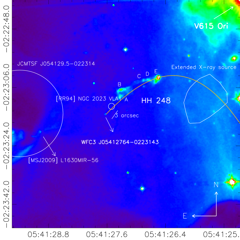
Figure 6: High-contrast HST/WFC3 H band image centered at HH 248 (Obs. ID 11548, PI: S. Megeath). Different high-density knots are identified with capital letters. The circles mark radio sources identified in the literature. Their radius corresponds to the 1$\sigma$ positional error. The position of the extended X-ray source identified by us as the interaction of jet with the molecular cloud is also marked. The continuous line is the precession curve.

In the optical band, at an angular resolution of  0.3$\arcsec$, HH 248 shows a knotty structure with five clear blobs. Figure 6 shows an HST/WFC3 image in the H band (Obs. ID 11548, obs. date 2010-10-19, exp. time 2496.170 s, PI: S. Megeath (catalog ADS/Sa.HST#IB0L9M010)). A very faint source (WFC3 J05412764-0223143) is detected 3$\arcsec$ to the South-East of the radio source [RR94] NGC 2023 VLA1 reported by Rodriguez & Reipurth (1994), at the position ($\alpha$, $\delta$) = (05^h 41^m 27.64^s, -02$\arcdeg$ 23$\arcmin$ 14.3$\arcsec$). WFC3 J05412764-0223143 is connected to HH 248 by a filamentary structure. WFC3 J05412764-0223143 is very likely the driving source of HH 248. Its magnitude in the F160W filter of the HST/WFC3 determined by us (see bellow) is $\sim 23.5$ mag, corresponding to a flux $F_{\nu}=0.46\pm 0.01$ $\mu$Jy. Compared to the fluxes determined for the knots (see Table 2) this value is between two and three orders of magnitude lower. WFC3 J05412764-0223143 must be highly absorbed, with $A_{\mathrm{V}}>13$ mag according to its observed magnitude in the F160W filter. To determine the fluxes of WFC3 J05412764-0223143 and the knots of HH 248, we performed aperture photometry in the pipeline processed data were obtained from the Mikulski Archive for Space Telescopes (MAST) using the DAOPHOT package (Stetson, 1987). An aperture radius of $1\arcsec$ was used in each case to prevent contamination from other close knots, whose typical separation is $\sim 2\arcsec$. We notice that a $1\arcsec$-radius extraction region encircles more than the 95% of each bright knot even for the case of knot E. Sky background value was fixed for subtraction. This value was estimated from the surroundings of the jet. An aperture correction was applied following the guidelines of the WFC3 instrument.

Table 2: WFC3 F160W photometry of the knots and their probable driving source.

Source	AB	Fν
	(mag)	($\mu$Jy)
J05412764-0223143	23.49 $\pm$ 0.18	0.46 $\pm$ 0.01
A	18.21 $\pm$ 0.01	58.96 $\pm$ 0.09
B	17.99 $\pm$ 0.01	72.17 $\pm$ 0.10
C	18.95 $\pm$ 0.02	29.88 $\pm$ 0.06
D	18.42 $\pm$ 0.01	48.71 $\pm$ 0.08
E	16.56 $\pm$ 0.01	270.16 $\pm$ 0.19

The chain of knots in HH 248 follows a curve path typical of precessed jets (e.g. Frank et al., 2014). In Figure 6 we show a simple fit of a precession curve (e.g. Masqué et al., 2012) to the knots and the IR source. The curve passes through the X-ray source. Hence, in the scenario proposed by us, the X-ray source is the bow shock produced by the encounter with a dense cloud of the jet flowing from WFC3 J05412764-0223143.

5 Simulations for HH 248

Table 3: Initial physical conditions in the jet, the ambient (ISM) and the wall.

Parameter	Value
Jet
Density	500 cm-3
Temperature	$10^{4}$ K
Velocity	$1.35\times 10^{3}$ km s-1
ISM
Dentity	50 cm-3
Temperature	$10^{5}$ K
Wall
Dentity	$5\times 10^{3}$ cm-3
Temperature	$10^{3}$ K

For our problem, we adopted a density of $5\times 10^{3}$ cm^-3 for the wall as a lower limit, based of measurements of the density in the surroundings of the Horsehead Nebula, where HH 248 is located (Habart et al., 2005). Then we scaled the density of the jet to have a light jet traveling through the ISM ($n_{\mathrm{jet}}/n_{\mathrm{ISM}}=10$) and a heavy jet through the wall ($n_{\mathrm{jet}}/n_{\mathrm{wall}}=0.1$). Pressure equilibrium is imposed. As a consequence, the temperatures of the three regions are fixed. We assume an initial temperature for the jet of $10^{4}$ K. Thus, the temperatures of the ISM and the wall are, respectively, $10^{5}$ and $10^{3}$ K. Table 3 summarizes the parameters of our model. Initially, the jet is defined as a homogeneous cylinder with size $r\sim 100$ AU and $z\sim 1000$ AU. The distance between the jet’s base and the dense cloud is kept as in Section 2. The actual projected distance between the X-ray source and WFC3 J05412764-0223143 is 9500-12000 AU, assuming a distance from the Earth between 350 and 450 pc as deduced from the measurements for $\sigma$ Orionis (e.g. Caballero, 2008).

Figure 7: Evolution of the jet’s intrinsic luminosity with time in the [0.3-10] keV energy band. The jet impacts onto the denser cloud at $t=1.1\times 10^{9}$ s.

The evolution of the jet’s luminosity with time is shown in Figure 7. X-ray luminosities were derived as discussed in Bonito et al. (2010b). In our space domain, the jet reaches the wall after $\sim 35$ years. Figure 7 shows that the intrinsic luminosity of the jet reaches $\sim 10^{31}$ erg s^-1 after its impact against the molecular cloud. However, during the first stage of the jet’s evolution, while the jet crosses the (less dense) ISM, its X-ray luminosity remains at a lower value ($\sim 10^{29}$ erg s^-1). An X-ray luminosity $>10^{30}$ erg s^-1 for the jet inside the high density molecular cloud is in agreement with the unabsorbed X-ray luminosity determined from the fit to the XMM-Newton data

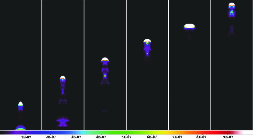
Figure 8: X-ray map of the jet after it reaches the high-density molecular cloud (wall). The period range is 40–65 yr with a time binning of 5 yr. The pixel size if 1 AU. The color scale is $10^{-7}$–$10^{-6}$ cnt s^-1 pixel^-1.

Figure 8 shows the X-ray evolution map of the jet as it travels through the high-density molecular cloud. Each panel corresponds to a time delay of five years. The first panel is for 30 yr from the beginning of the model run. Figure 9 shows the temperature (left panel) and the density (right panel) maps describing the jet/wall interaction.

The emission measure ($EM$) distribution near the end of the simulation (penultimate panel in Figure 8) shows a small bump at $T\sim 10^{6}$ K (see Figure 10). The mean value of the $EM$ obtained from our simulations is compatible with the $EM$ obtained from the fit to the X-ray data ($\sim 2\times 10^{53}$ cm^-3). Note that the $EM(T)$ at temperature $<1$ MK shows a plateau analogous to that found by BOP07 in their simulations. This is mainly due to the radiative losses that are very efficient at $T\sim 10^{5}$ K and that cause a bump of $EM(T)$ at $T\sim 10^{4}$ K. We have verified this point by comparing simulations either with or without the radiative losses.

   

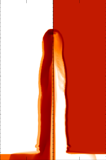
Figure 9: Enlargement of the temperature (left panel) and density (right panel) maps derived from our simulations describing the jet/wall interaction (at 45 yr from the beginning of the simulation). The complete movie of the evolution is also available as online material.

6 Discussion and conclusions

In this work, we studied the scenario of a stellar jet impacting a molecular cloud from a HD modeling approach. In particular, we simulated supersonic stellar jets moving through ISM medium that is less dense than the jet encountering a dense molecular cloud. Hence, the jet becomes underdense inside the molecular cloud. From previous results (e.g. BOP07), X-ray emission is expected when the jet is lighter than the surrounding medium, while it is not when the jet is heavier than the ambient.

Our simulations explore the parameter space: jet’s velocity, ISM density and molecular cloud density. The scenario of a light jet that impacts a dense cloud may be typical of some stellar jets observed in star-forming regions. In particular, this scenario is possibly occurring for HH 248. Our main goal is to investigate whether such an impact may produce X-ray emission from the jet.

Our results from the simulations indicate that jets with $v_{\mathrm{jet}}\gtrsim 700$ km s^-1 can reach temperatures of several MK after impacting the dense molecular cloud. This result is in agreement with detection of X-ray emission from the jet. In contrast, low velocity jets do not reach such temperatures. We find a clear trend of increasing temperature after impact with increasing the jet’s velocity, independently of the density ratio between the jet and the dense molecular cloud.

We used these results to investigate the possible origin and evolution of HH 248, including the possibility of X-ray emission after encountering the high density region at the base of the Horsehead Nebula. From our multiwavelength analysis of the HH object, we reveal the probable driving source of the jet, which is a highly absorbed point-like source detected only in a deep H-band image with the HST/WFC3. From the WFC3 image, we identify five dense knots that are not fully aligned with WFC3 J05412764-0223143. We used them to determine the parameters of the precession of the jet associated with HH 248. The fitted precession curve pass through the extended X-ray source named by López-García et al. (2013) as Src. 12. We conclude that this X-ray source is the front shock of the jet that created HH 248.

Figure 10: Emission measure distribution ($EM$) as a function of temperature ($T$) for the penultimate panel of Figure 8, at a time of 25 yr after the interaction of the jet with the molecular cloud (60 yr from the beginning of our simulation).

From our X-ray data analysis, we discard the possibility that the extended X-ray source were part of the PSF of the classical T Tauri star V615 Ori, also detected in the XMM-Newton as $\sim 30\arcsec$. In particular, the column density determined for this source is one order of magnitude higher than that determined for V615 Ori by López-García et al. (2013). We propose a scenario for HH 248 in which the jet, which moves through the ISM, reaches a region of much higher density. This region may be identified with the ionization front IC 434 that runs south from the NGC 2024 star-forming region and contains the Horsehead Nebula (Barnard 33). In this scenario, the jet, which is heavier than the ISM but lighter than the molecular cloud, emits in X-rays when it reaches the denser cloud. Hence, the X-ray emission from the jet would be produced far from the jet base, contrarily to other cases (see Section 1). In the classification given by Bonito et al. (2010b), luminous X-ray jets detected at large distances from their driving source seem to be associated with high-mass stars. In our case, the location of the X-ray emission from the jet would not be related to the mass of the driving source but to the change in the conditions of the ISM. This is an excellent test case to check the idea that detectable X-ray emission from stellar jets is produced if the jet travels through a denser environment (BOP07).

From our results, we conclude that X-ray emission from the impact of a stellar jet with a dense cloud is feasible. Deep X-ray observations of HH objects in nearby star forming-regions may reveal other cases similar to HH 248. New X-ray observations are needed to determine precisely some parameters of the X-ray counterpart of the jet.

References

- Albertazzi et al. (2014) Albertazzi, B., Ciardi, A., Nakatsutsumi, M., et al. 2014, Science, 346, 325
- Anglada & Rodríguez (2002) Anglada, G., & Rodríguez, L. F. 2000, Rev. Mexicana Astron. Astrofis., 38, 13
- Arnaud (1996) Arnaud, K. A. 1996, Astronomical Data Analysis Software and Systems V, 101, 17
- Arnaud (2004) Arnaud, K. 2004, Bulletin of the American Astronomical Society, 36, 934
- Bally et al. (2003) Bally, J., Feigelson, E., & Reipurth, B. 2003, ApJ, 584, 843
- Bonito et al. (2004) Bonito, R., Orlando, S., Peres, G., Favata, F., & Rosner, R. 2004, A&A, 424, L1
- Bonito et al. (2007) Bonito, R., Orlando, S., Peres, G., Favata, F., & Rosner, R. 2007, A&A, 462, 645 (BOP07)
- Bonito et al. (2010a) Bonito, R., Orlando, S., Peres, G. et al. 2010a, A&A, 511, A42
- Bonito et al. (2010b) Bonito, R., Orlando, S., Miceli, M., et al. 2010b, A&A, 517, A68
- Bonito et al. (2011) Bonito, R., Orlando, S., Miceli, M., et al. 2011, ApJ, 737, 54
- Caballero (2008) Caballero, J. A. 2008, MNRAS, 383, 750
- Cash (1979) Cash, W. 1979, ApJ, 228, 939
- Coffey et al. (2012) Coffey, D., Rigliaco, E., Bacciotti, F., Ray, T. P., & Eislöffel, J. 2012, ApJ, 749, 139
- Colella & Woodward (1984) Colella, P., & Woodward, P. R. 1984, Journal of Computational Physics, 54, 174
- Di Francesco et al. (2008) Di Francesco, J., Johnstone, D., Kirk, H., MacKenzie, T., & Ledwosinska, E. 2008, ApJS, 175, 277
- Favata et al. (2002) Favata, F., Fridlund, C. V. M., Micela, G., Sciortino, S., & Kaas, A. A. 2002, A&A, 386, 204
- Favata et al. (2006) Favata, F., Bonito, R., Micela, G., et al. 2006, A&A, 450, L17
- Ferreira et al. (2006) Ferreira, J., Dougados, C., & Cabrit, S. 2006, A&A, 453, 785
- Frank et al. (2014) Frank, A., Ray, T. P., Cabrit, S., et al. 2014, arXiv:1402.3553
- Fryxell et al. (2000) Fryxell, B., Olson, K., Ricker, P., et al. 2000, ApJS, 131, 273
- Gómez de Castro & von Rekowski (2011) Gómez de Castro, A. I., & von Rekowski, B. 2011, MNRAS, 411, 849
- Grosso et al. (2006) Grosso, N., Feigelson, E. D., Getman, K. V., et al. 2006, A&A, 448, L29
- Güdel et al. (2005) Güdel, M., Skinner, S. L., Briggs, K. R., et al. 2005, ApJ, 626, L53
- Güdel et al. (2008) Güdel, M., Skinner, S. L., Audard, M., Briggs, K. R., & Cabrit, S. 2008, A&A, 478, 797
- Habart et al. (2005) Habart, E., Abergel, A., Walmsley, C. M., Teyssier, D., & Pety, J. 2005, A&A, 437, 177
- Kastner et al. (2005) Kastner, J. H., Franz, G., Grosso, N., et al. 2005, ApJS, 160, 511
- Koenigl (1991) Koenigl 1991, ApJ, 370, L39
- Lawrence et al. (2007) Lawrence, A., Warren, S. J., Almaini, O., et al. 2007, MNRAS, 379, 1599
- Linsky et al. (2007) Linsky, J. L., Gagné, M., Mytyk, A., McCaughrean, M., & Andersen, M. 2007, ApJ, 654, 347
- Löhner (2008) Löhner, R. 2008, Applied Computational Fluid Dynamics Techniques: An Introduction Based on Finite Element Methods (2nd ed.; England: John Wiley & Sons Ltd.)
- López-García et al. (2013) López-García, M. A., López-Santiago, J., Albacete-Colombo, J. F., Pérez-González, P. G., & de Castro, E. 2013, MNRAS, 429, 775
- MacNeice et al. (2000) MacNeice, P., Olson, K. M., Mobarry, C., de Fainchtein, R., & Packer, C. 2000, Comput. Phys. Comm., 126, 330
- Malin et al. (1987) Malin, D. F., Ogura, K., & Walsh, J. R. 1987, MNRAS, 227, 361
- Masqué et al. (2012) Masqué, J. M., Girart, J. M., Estalella, R., Rodríguez, L. F., & Beltrán, M. T. 2012, ApJ, 758, L10
- Matsakos et al. (2008) Matsakos, T., Tsinganos, K., Vlahakis, N., et al. 2008, A&A, 477, 521
- Matsakos et al. (2009) Matsakos, T., Massaglia, S., Trussoni, E., et al. 2009, A&A, 502, 217
- Mookerjea et al. (2009) Mookerjea, B., Sandell, G., Jarrett, T. H., & McMullin, J. P. 2009, A&A, 507, 1485
- Orellana et al. (2012) Orellana, M., Bonito, R., López-Santiago, J., Albacete Colombo, J. F., & Miceli, M. 2012, Boletin de la Asociacion Argentina de Astronomia La Plata Argentina, 55, 187
- Pravdo et al. (2001) Pravdo, S. H., Feigelson, E. D., Garmire, G., et al. 2001, Nature, 413, 708
- Pravdo et al. (2004) Pravdo, S. H., Tsuboi, Y., & Maeda, Y. 2004, ApJ, 605, 259
- Pravdo et al. (2009) Pravdo, S. H., Tsuboi, Y., Suzuki, Y., Thompson, T. J., & Rebull, L. 2009, ApJ, 690, 850
- Reipurth & Bally (2001) Reipurth, B., & Bally, J. 2001, ARA&A, 39, 403
- Reipurth et al. (2004) Reipurth, B., Rodríguez, L. F., Anglada, G., & Bally, J. 2004, AJ, 127, 1736
- Rodriguez & Reipurth (1994) Rodriguez, L. F., & Reipurth, B. 1994, A&A, 281, 882
- Schneider et al. (2013) Schneider, P. C., Eislöffel, J., Güdel, M., et al. 2013, A&A, 550, L1
- Skinner et al. (2011) Skinner, S. L., Audard, M., Güdel, M. 2011, ApJ, 737, 19
- Smith et al. (2001) Smith, R. K., Brickhouse, N. S., Liedahl, D. A., & Raymond, J. C. 2001, Spectroscopic Challenges of Photoionized Plasmas, 247, 161
- Staff et al. (2014) Staff, j. e., Koning, N., Ouyed, R., Thompson, A., & Pudritz, R. E. 2014, arXiv_1411.3440v1
- Stelzer et al. (2009) Stelzer, B., Hubrig, S., Orlando, S., et al. 2009, A&A, 499, 529
- Stetson (1987) Stetson, P. B. 1987, PASP, 99, 191
- Stute et al. (2014) Stute, M., Gracia, J., Vlahakis, N., et al. 2014, MNRAS, 439, 3641
- Tsujimoto et al. (2004) Tsujimoto, M., Koyama, K., Kobayashi, N., et al. 2004, PASJ, 56, 341
- Velusamy et al. (2014) Velusamy, T., Langer, W. D., & Thompson, T. 2014, ApJ, 783, 6