Dynamics of Cloud Features on Uranus

Abstract

Near-infrared adaptive optics imaging of Uranus by the Keck 2 telescope during 2003 and 2004 has revealed numerous discrete cloud features, 70 of which were used to extend the zonal wind profile of Uranus up to 60^∘ N. We confirmed the presence of a north-south asymmetry in the circulation (Karkoschka, Science 111, 570-572, 1998), and improved its characterization. We found no clear indication of long term change in wind speed between 1986 and 2004, although results of Hammel et al. (2001, Icarus 153, 229-235) based on 2001 HST and Keck observations average $\sim$10 m/s less westward than earlier and later results, and 2003 observations by Hammel et al. (2005, Icarus 175, 534-545) show increased wind speeds near 45^∘N, which we don’t see in our 2003-2004 observations. We observed a wide range of lifetimes for discrete cloud features: some features evolve within $\sim$1 hour, many have persisted at least one month, and one feature near 34^∘ S (termed S34) seems to have persisted for nearly two decades, a conclusion derived with the help of Voyager 2 and HST observations. S34 oscillates in latitude between 32^∘ S and 36.5^∘ S, with a period of $\sim$1000 days, which may be a result of a non-barotropic Rossby wave. It also varied its longitudinal drift rate between -20^∘/day and -31^∘/day in approximate accord with the latitudinal gradient in the zonal wind profile, exhibiting behavior similar to that of the DS2 feature observed on Neptune (Sromovsky et al., Icarus 105, 110-141, 1993). S34 also exhibits a superimposed rapid oscillation with an amplitude of 0.57^∘ in latitude and period of 0.7 days, which is approximately consistent with an inertial oscillation.

1. Introduction

Among the outer planets, Uranus is unique in two key parameters affecting atmospheric dynamics. First, it has almost a complete absence of internal heat flux. From Voyager IRIS observations Pearl et al. (1990) estimated the ratio of emission to absorbed sunlight to be $E$ = 1.06$\pm$0.08, while the corresponding ratio for Neptune is 2.61$\pm$0.28 (Pearl et al. 1991). This result, which may not be invariant, does suggest that solar energy provides the overwhelming drive for atmospheric dynamics on Uranus. Second, Uranus’ rotational axis is nearly in the plane of its orbit. This produces an extreme in the fractional seasonal variation of local solar flux on Uranus, and thus raises the question of what seasonal response might be generated. However, the long radiative time constant of Uranus, which is longer than its 84-year orbital period (Flasar et al. 1987), suggests that the response should be strongly damped. Allison et al. (1991) concluded that at levels below the visible cloud tops, there would be a thermal phase lag of nearly a full Uranian season. Using a radiative-convective model Wallace (1983) estimated that annual variations would be $\sim$5 K at the poles and $\sim$0.5 K at the equator. Friedson and Ingersoll (1987) found that including dynamical heat transports by baroclinic eddies resulted in peak-to-peak temperature variations that were about half those estimated by Wallace and in better agreement with IRIS measurements at the time of the Voyager encounter (Hanel et al. 1986).

The bland appearance of Uranus at the time of the Voyager encounter seemed consistent with the lack of an internal heat source and the long radiative time constant. After months of Voyager 2 imaging, only eight eight discrete cloud features could be defined well enough to use as tracers of Uranus’ zonal circulation (Smith et al. 1986). Seven of these were between 27^∘S and 40^∘S, and one near 70^∘S was visible only in UV images. These had relatively low contrast, ranging from from less than 1% in violet to about 7% in the red filter. The features were also very small, making them difficult to observe in moderate resolution images. Subsequent HST imaging at similar wavelengths was thus understandably not very productive. The situation improved significantly in 1997 when the HST NICMOS instrument made possible near IR imaging of Uranus at high spatial resolution. Karkoschka (1998) identified ten new discrete cloud features in the 1997 NICMOS images and additional features were observed in 1998 images (Karkoschka and Tomasko 1998). The maximum contrast of northern cloud features was obtained at 1.87 $\mu$m, reaching 180% in the raw NICMOS images. Near IR imaging at the IRTF in 1998 and 1999 also revealed discrete cloud features on Uranus (Forsythe et al. 1999; Sromovsky et al. 2000). These were the first discrete features seen in groundbased digital images of Uranus, and the 1999 feature was the brightest ever recorded at 1.7 $\mu$m, comprising $\sim$5% of the disk-integrated brightness. Recent groundbased observations with the Keck telescope AO system combined exceptional light gathering capabilities and spatial resolution to reveal a great many more discrete features (Hammel et al. 2001, de Pater et al. 2002, Hammel et al. 2005), permitting improved determinations of the Uranus wind profile, especially at latitudes not previously visible.

Karkoschka (1998) argued that the growing abundance of discrete cloud features did not represent a significant change in activity of Uranus, but was due mainly to a change in view angle and improved wavelength selection. Although his observations had relatively sparse sampling, he was able to identify cloud features over long time intervals from which highly accurate drift rates (or wind speeds) could be defined. It appeared that cloud features on Uranus had generally very long lifetimes compared to cloud features on Neptune, few of which can be found on subsequent rotations (Limaye and Sromovsky 1991). On the other hand, the Wallace (1983) model predicts seasonal variations in convective activity, with most of the convection occurring between the winter solstice and shortly after equinox (2007). The Friedson and Ingersoll (1987) model predicts that during the 1994-2007 period, the temperature contrast between north and south should be near a maximum. It remains to be understood whether the small temperature variations these models predict can explain what is turning out to be significant north-south asymmetries in the dynamics and motions of discrete cloud features.

New groundbased images we obtained in 2003 and 2004 from the Keck telescope provide a new abundance of discrete cloud features that we use to gain a better understanding of Uranus’ atmospheric dynamics. In the following we discuss their morphologies, motions, and evolution, and include in the analysis results from Voyager and HST observations. We extend the zonal wind observations up to 60^∘ N, and show that the north-south asymmetry of Uranus’ zonal circulation is mainly confined to mid latitudes. We were able to determine highly accurate drift rates by tracking features that persisted for at least one month. We identify a broad range of evolutionary time scales for discrete cloud features, and show that one feature probably existed for two decades or more, and has exhibited regular oscillations in latitude and longitude, which can plausibly be associated with both Rossby waves and inertial oscillations.

2. Observations

2.1. Recent Keck Observations

Using the NIRC2 camera on the Keck 2 telescope we observed Uranus and Neptune on 15 and 16 July 2003, on 11 and 12 July 2004, and on 11 and 12 August 2004. The observing geometry for each date is summarized in Table 1, for 12:00 UT. Most of our images were made with broadband J, H, and K’ filters using the NIRC2 Narrow Camera. After geometric correction, the angular scale of this camera is 0.009942^′′/pixel (NIRC2 General Specifications web page: http://alamoana.keck.hawaii.edu/inst/nirc2/ genspecs.html). The times, filters, exposures, and airmass values for these broadband observations are provided in Tables II and III. The exposures per coadd were chosen to avoid saturation of Uranus satellite images so that they could be used for short-term photometric references. The total exposures are less than optimal and represent a compromise resulting from frequent alternation between Uranus and Neptune imaging during each observing run. Images of Hammel et al. (2005) provide better S/N ratios as a result of longer exposures. The central wavelengths and bandwidths of the filters used here are given in Table 4. The pressure levels in Uranus’ atmosphere sensed by these filters is indicated in Fig. 1. We also acquired a small number of narrow-band images in 2004 to provide a cleaner constraint on vertical cloud structure. These are presented in a separate paper (Sromovsky and Fry 2005), hereafter referred to as Paper II.

To assess Adaptive Optics (AO) performance, we measured stellar images, satellite images and epsilon ring cross sections (this ring is visible in Fig. 2). During 15 August 2003 most observations achieved effective seeing of 0.052^′′-0.09^′′ and was mostly in the range 0.061^′′-0.13^′′ on the following night. During 11 July 2004 seeing was excellent, typically 0.05^′′-0.06^′′ with AO turned on. During 11 August 2004, raw seeing was about 0.5^′′ in K and effective seeing at 2.15$\mu$m with AO active reached 0.055^′′. Natural seeing during 12 August 2004 reached 0.43^′′. With AO on we measured 0.07^′′-0.08^′′ in H stellar images (of the relatively faint star FS34). Later measurements of a brighter star (Elias G 158-27) obtained FWHM values of 0.063^′′-0.070^′′ for H and 0.08^′′-0.090^′′ for J.

Table 1Observing geometry for 2003 and 2004 Keck observations.

	Range, AU	Distance, AU	Centric	Centric	Phase
Date (12UT)	(Earth-Uranus)	(Sun-Uranus)	Solar Lat.,∘	Earth Lat.,∘	Angle,∘	MJD
15 AUG 2003	19.03	20.03	-16.69	-16.24	0.46	52866.5
16 AUG 2003	19.03	20.03	-16.68	-16.28	0.41	52867.5
11 JUL 2004	19.34	20.05	-13.18	-11.07	2.13	53197.5
12 JUL 2004	19.33	20.05	-13.17	-11.10	2.09	53198.5
11 AUG 2004	19.08	20.05	-12.85	-12.03	0.82	53228.5
12 AUG 2004	19.07	20.05	-12.84	-12.07	0.77	53229.5

Table 2Uranus observation list for 2003.

Start time	Filter	Itime $\times$coadds	airmass	Start time	Filter	Itime $\times$coadds	airmass
	15aug03UT				16aug03UT
12:21:05	H	15 $\times$ 4	1.25	10:04:22	H	15 $\times$ 4	1.21
12:22:51	H	15 $\times$ 4	1.26	12:18:23	H	15 $\times$ 4	1.26
12:32:58	Kp	12 $\times$ 10	1.28	12:22:55	J	15 $\times$ 4	1.27
12:41:25	H	15 $\times$ 4	1.30	12:28:17	Kp	12 $\times$ 20	1.28
12:48:13	H	15 $\times$ 4	1.32	12:41:51	H	15 $\times$ 4	1.32
12:57:47	J	15 $\times$ 4	1.36	12:46:38	J	15 $\times$ 4	1.33
13:04:22	H	15 $\times$ 2	1.38	12:51:59	H	15 $\times$ 4	1.35
				12:56:16	H	15 $\times$ 4	1.37
				13:00:56	J	15 $\times$ 4	1.38

Table 3Uranus observation list for 2004.

Start time	Filter	Itime $\times$coadds	airmass	Start time	Filter	itime $\times$coadds	airmass
	11jul04UT				12jul04UT
11:22:15	J	15 $\times$ 4	1.40	10:30:35	J	15 $\times$ 4	1.69
11:30:32	H	15 $\times$ 4	1.37	10:42:40	J	15 $\times$ 4	1.60
11:34:46	Kp	24 $\times$ 10	1.35	10:49:23	H	15 $\times$ 4	1.55
12:37:57	J	15 $\times$ 4	1.19	11:49:24	J	15 $\times$ 4	1.29
12:42:33	H	15 $\times$ 4	1.19	11:54:22	Kp	24 $\times$ 10	1.27
13:39:50	J	15 $\times$ 4	1.15	12:05:51	H	15 $\times$ 4	1.24
13:45:22	H	15 $\times$ 4	1.15	13:04:50	J	15 $\times$ 4	1.16
14:13:48	H	15 $\times$ 4	1.17	13:09:47	Kp	24 $\times$ 10	1.16
14:45:50	J	15 $\times$ 4	1.21	13:36:59	H	15 $\times$ 4	1.15
14:50:35	H	15 $\times$ 4	1.22	14:04:34	J	15 $\times$ 4	1.16
14:54:50	Kp	24 $\times$ 10	1.23	14:09:18	H	15 $\times$ 4	1.17
15:06:37	J	15 $\times$ 4	1.25	14:38:09	J	15 $\times$ 4	1.20
15:11:09	H	15 $\times$ 4	1.26	14:44:47	H	15 $\times$ 4	1.21
15:15:36	Kp	24 $\times$ 10	1.28	14:49:05	Kp	24 $\times$ 10	1.22
15:27:07	H	15 $\times$ 4	1.31	15:00:29	Kp	24 $\times$ 10	1.25
15:31:27	H	15 $\times$ 4	1.32	15:07:08	J	15 $\times$ 4	1.26
				15:11:42	H	15 $\times$ 4	1.28
				15:16:14	Kp	24 $\times$ 10	1.29
				15:27:37	H	15 $\times$ 4	1.33
				15:32:23	J	15 $\times$ 4	1.34
	11aug04UT				12aug04UT
07:11:27	J	15 $\times$ 4	3.00	07:24:55	J	15 $\times$ 4	2.53
07:18:00	Kp	24 $\times$ 10	2.80	07:29:45	H	15 $\times$ 4	2.43
07:29:45	H	15 $\times$ 4	2.51	07:59:30	J	15 $\times$ 4	1.96
08:08:48	J	15 $\times$ 4	1.89	08:04:32	Kp	24 $\times$ 5	1.90
08:25:04	H	15 $\times$ 4	1.73	08:11:14	H	15 $\times$ 4	1.83
09:30:34	J	15 $\times$ 4	1.35	09:04:37	J	15 $\times$ 4	1.44
09:44:07	Kp	24 $\times$ 10	1.30	09:09:38	Kp	24 $\times$ 5	1.42
09:53:46	H	15 $\times$ 4	1.28	09:16:53	H	15 $\times$ 4	1.39
10:15:35	J	15 $\times$ 4	1.23	09:46:18	J	15 $\times$ 4	1.29
10:20:30	H	15 $\times$ 4	1.22	09:51:01	Kp	24 $\times$ 10	1.27
11:32:57	J	15 $\times$ 4	1.16	10:02:39	H	15 $\times$ 4	1.24
11:37:50	Kp	24 $\times$ 10	1.16	11:11:05	J	15 $\times$ 4	1.16
11:49:33	H	15 $\times$ 4	1.16	11:20:48	H	15 $\times$ 4	1.16
12:45:27	J	15 $\times$ 4	1.22	12:41:43	J	15 $\times$ 4	1.22
12:50:24	Kp	24 $\times$ 10	1.23	12:46:22	H	15 $\times$ 4	1.23
13:02:11	H	15 $\times$ 4	1.26	13:28:42	J	15 $\times$ 4	1.36
14:02:14	J	15 $\times$ 4	1.49	13:33:25	Kp	24 $\times$ 10	1.37
14:15:01	H	15 $\times$ 4	1.57	13:45:27	H	15 $\times$ 4	1.43
14:19:37	Kp	24 $\times$ 5	1.60	13:50:42	J	15 $\times$ 4	1.45
				13:55:59	Kp	24 $\times$ 10	1.48
				14:09:09	H	15 $\times$ 4	1.55
				14:13:51	H	15 $\times$ 4	1.59

Figure 1.— Penetration of sunlight into the atmosphere of Uranus vs wavelength. Solid curves are shown for two-way vertical optical depths of 1, 2, and 4 from CH₄ and H₂ absorption. Dotted curves show the same optical depths for Rayleigh scattering, except for $\lambda>1\mu$m, where curves are shown for Rayleigh optical depths of 0.1 and 0.01. Filter passbands for NIRC2 are indicated by horizontal bars. Voyager, WFPC2, NICMOS, and ACS filters are shown as system throughput curves, normalized to unity at their peaks. See Table 4 for additional filter information. Horizontal dashed lines indicate the location of the putative CH₄ cloud at 1.2 bars (Lindal et al. 1987), and the putative H₂S cloud at 3.1 bars (Baines et al. 1995).

2.2. Voyager and HST Observations

The 1986 Voyager 2 and HST images we used for tracking a feature near 34^∘S are listed in Section 5. We used Voyager 2 Wide-Angle orange filter images, with spectral characteristics given in Table 3 and in Fig. 1. The Voyager images were taken at a time when very little of the northern hemisphere was illuminated. The HST WFPC2, NICMOS, and ACS imagery we used for the same purpose are listed in Section 5. Their filter characteristics are also given in Table 3 and Fig. 1.

2.3. Image Processing and Navigation

Our Keck images were dark-subtracted, flat-fielded, geometrically corrected, and then navigated. Differences between lamp-on and lamp-off dome image triplets were median filtered and normalized by the median difference to define the flat-field correction. The significant geometric distortions in the NIRC2 images were removed using an inversion of the 10-term cubic polynomial given in the NIRC2 pre-ship test report (Thompson et al. 2001). We made use of the SPICELIB toolkit (Acton 1996) to generate ephemeris information concerning the orientation of the planet’s pole vector, the range to the planet, and the latitude and longitude of the observer (the point at which a vector from the planet center to the observer intersects the surface). We used standard 1-bar radii of $r_{\mathrm{eq}}$ = 25,559 km and $r_{\mathrm{pol}}$ = 24,973 km and a longitude system based on a 17.24-h period (Siedelmann et al. 2002). We spot checked image orientation values in the NIRC2 file header by measuring the positions of Uranian satellites, and found good agreement. We determined planet center coordinates by fitting a projected planet limb to maximum gradient limb points. The combined effect of navigation errors and other cloud tracking errors is approximately 1 narrow camera pixel rms, which is estimated from the image-to-image scatter found in the plots of discrete cloud position versus time. In describing positions we use both planetocentric latitude ($\phi$), which is the angle above the equatorial plane measured from the planet center, and planetographic latitude ($\phi_{\mathrm{pg}}$), which is the angle between the local normal and the equatorial plane. These are related through the equation $\tan\phi_{\mathrm{pg}}=(r_{\mathrm{eq}}/r_{\mathrm{pol}})^{2}\tan\phi$.

HST image processing and navigation proceeded along the lines described by Sromovsky et al. (2001), except that we used the same navigation procedure described above. Voyager 2 Uranus images were processed using USGS ISIS software (http://isis.astrogeology.usgs.gov) to correct for vidicon geometric distortions and to remove reseau features. The images were navigated as described above.

3. Atmospheric Circulation Results

Before we present our wind results, it is worth addressing a potential point of confusion in applying earth-based dynamical arguments to Uranus. Defining the rotational pole of Uranus by the right hand rule places it 98^∘ from its orbital pole. Because the tilt puts this pole south of the invariable plane of the solar system, IAU convention makes this the south pole of the planet (Seidelmann 2002). On Uranus, winds that blow in the same direction as the planet rotates are thus westward, while on Neptune the prograde winds are eastward. Because planetographic longitude always increases with time by definition, it is equal to west longitude on Neptune, but east longitude on Uranus. To facilitate the application of existing dynamical arguments and intuition developed from studies of Earth, Jupiter, Saturn, Neptune, and Mars, it is useful to define dynamically equivalent directions for Uranus: dynamical north = IAU south and dynamical east = IAU west. We follow Allison et al. (1991) and Hammel et al. (2001, 2005) in using prograde (IAU westward or dynamical eastward) winds as positive winds on Uranus.

3.1. Cloud-tracked winds from 2003 and 2004

A sampling of the discrete cloud features we used to track atmospheric motions is provided for each of the three observing runs in Figs. 2, 3, and 4. Images in the top row of each figure were obtained using the K^′ filter and the middle row with the H filter, which provides somewhat better contrast than the J filter, presumably due to the reduced contribution of Rayleigh scattering at the longer wavelengths of the H filter (see Fig. 1). The bottom row in each figure displays a high-pass filtered version of the H image to enhance contrast for subtle cloud features. All the encircled cloud targets were observed on multiple images and were used to determine drift rates and wind speeds. Only the higher altitude cloud features are visible in the K^′ image. In Paper II we show that the highest of these features reach to $\sim$200 mb. The northern boundary of the southern bright band is also a point at which discrete cloud features develop (108 and 129 in Fig. 3). We have also seen discrete clouds at this boundary in 1998 NICMOS images. In the equatorial regions, cloud features are particularly fuzzy and of low contrast (see 306, 312, and 311 in Fig. 2). Hammel et al. (2004) tracked six of these features within 2^∘ of the equator. We were able to track six between 0^∘N and 10^∘N.

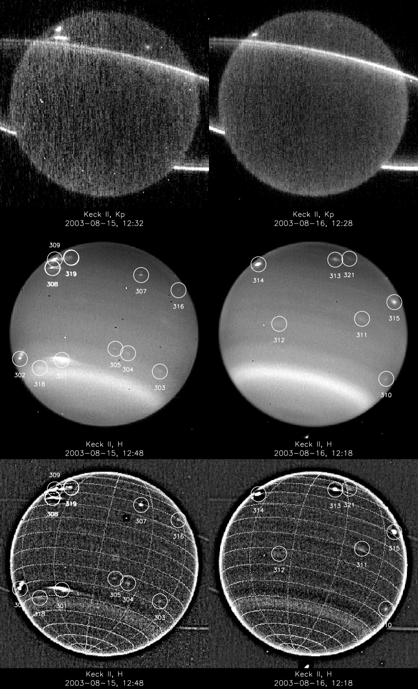
Figure 2.— Sample images of opposite hemispheres of Uranus in August 2003: K^′ images in upper row, H images in middle row, and high-pass filtered H images in bottom row, where latitude grid lines are at 10^∘ intervals, and longitude grid lines are at 30^∘ intervals. Target numbers are used to reference results in Table 5.

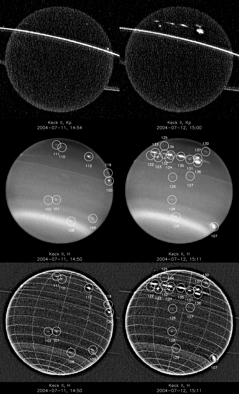
Figure 3.— Same as Fig. 2, except images are from July 2004 observations.

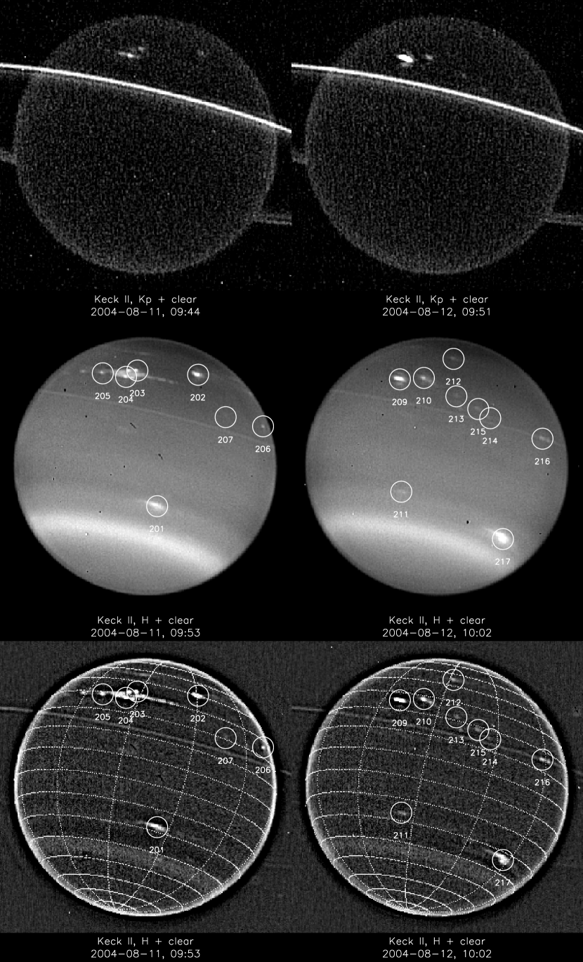
Figure 4.— Same as Fig. 2, except images are from August 2004 observations.

Each of our Keck runs provided observations on two successive nights, between which Uranus undergoes 1.39 rotations. As a result, there were only a few cloud targets seen on both nights of each observing run. These provided the highest wind speed accuracy, of the order of 1.7 to 8 m/s. Most targets were followed during only a single transit on one night, for which the best accuracy is about 13-15 m/s, for a target tracked over about 5 hours. The longest tracking time within a single transit was 5.5 hours. These estimated uncertainties in the zonal winds are of the same order as uncertainties in the meridional winds, although meridional wind speeds are much smaller. Because we could not resolve any systematic meridional motion for features observed on only one transit, meridional wind speeds are not tabulated. However, rather substantial meridional excursions of $\pm$2.1^∘ of latitude were observed for a long-lived feature near 34^∘S, which is discussed in detail in a Section 5.2. Models imply that this feature regularly reaches peak meridional speeds of 28 m/s, but varies so rapidly that it is difficult to resolve by direct measurement.

Table 4Spectral responsivity characteristics for NIRC2, Voyager 2, WFPC2, ACS, and NICMOS filter bands we used.

		Central	Bandpassa,	cut-onb,	cut-offb,
Instrument	Filter	$\lambda$, $\mu$m	$\mu$m	$\mu$m	$\mu$m
NIRC2c	J	1.248	0.163	1.166	1.330
NIRC2c	H	1.633	0.296	1.485	1.781
NIRC2c	K′	2.124	0.351	1.948	2.299
Voyager 2d	WA Orange	0.60	0.04	0.58	0.62
WFPC2e	791W	0.790	0.130	0.710	0.865
WFPC2e	F850LP	0.909	0.106	0.85	0.956
WFPC2e	F953N	0.954	0.005
ACSf	F814W	0.8333	0.251	0.708	0.959
ACSf	F775W	0.7764	0.1528	0.700	0.853
NICMOS NIC1g	F160W	1.603	0.399	1.40	1.80

^afull width at half maxima, except for WFPC2 which is effective bandpass.
^bhalf maximum point.
^cfrom www.alamoana.keck/hawaii.edu/inst/nirc2/filters.html.
^dfrom Danielson et al. (1981).
^efrom WFPC2 Instrument Handbook v 9.0, Oct. 2004.
^ffrom ACS Instrument Handbook v5.0, Oct. 2004.
^gfrom Appendix A, NICMOS Instrument Handbook v 7.0, Oct. 2004, system throughput.

In Tables 5 and 6, we provide a summary of discrete feature observations during August 2003 and during July and August 2004. These are a subset for which wind speed uncertainties are less than 60 m/s. Most of the errors are less than 40 m/s. These results are obtained by fitting individual longitude observations to a linear drift model, weighting individual observations by the inverse of their expected variances. The error estimates are computed in the pixel domain, and taken to be 1 pixel rms. As noted previously, this estimate incorporates tracking and image navigation errors. We made a systematic comparison of expected errors based on a 1-pixel position uncertainty from all sources with standard deviations from a linear longitude-vs-time regression line, and found generally good agreement. The 70 tabulated individual target winds are plotted in Fig. 5. The wind speed of 238$\pm$52 m/s at 60^∘N is for the northernmost and highest speed cloud so far tracked in the atmosphere of Uranus. However, this target is not visible in the sample images displayed in Fig. 3. Targets tend to cluster in narrow latitude bands, leaving gaps near 37^∘N and especially south of 42^∘S. The only discrete feature ever tracked in the latter region was seen only in Voyager 2 UV images (Smith et al., 1986). No features were tracked between 60^∘N and the terminator (73^∘ N in 2003 and 77^∘ N in 2004), which is at least partly due to poor viewing geometry.

Table 5Individual zonal wind determinations by cloud target (Northern Hemisphere).

Lat. ($\phi$)	Lat. ($\phi_{pg}$)	Drift rate (∘E/h)	u(m/s westward)	IDa	Nobs	$<\lambda>$(∘E)	$<$Mod. Julian Day$>$
59.52	60.38$\pm$0.54	-3.82$\pm$0.83	238$\pm$52	146	4	153.4	53198.60118
49.70	50.67$\pm$0.41	-2.53$\pm$0.45	202$\pm$36	148	3	337.4	53197.52743
47.44	48.42$\pm$0.39	-2.69$\pm$0.42	224$\pm$35	223	3	28.9	53228.48894
46.75	47.73$\pm$0.27	-2.21$\pm$0.28	187$\pm$23	141	6	152.0	53198.56881
45.84	46.83$\pm$0.26	-2.33$\pm$0.29	200$\pm$25	1111	6	9.7	53197.59845
45.02	46.01$\pm$0.34	-2.27$\pm$0.08	198$\pm$07	138	4	68.1	53197.83650
44.49	45.48$\pm$0.31	-2.16$\pm$0.32	190$\pm$28	2121	4	123.4	53229.40479
42.89	43.87$\pm$0.23	-1.44$\pm$0.26	130$\pm$24	110	6	18.9	53197.59845
42.37	43.35$\pm$0.30	-1.75$\pm$0.29	159$\pm$26	208	4	43.4	53228.51515
41.02	42.00$\pm$0.25	-1.51$\pm$0.25	141$\pm$24	125	5	142.3	53198.58176
40.04	41.01$\pm$0.22	-1.32$\pm$0.62	125$\pm$59	313	7	199.1	52867.52967
39.86	40.84$\pm$0.23	-1.47$\pm$0.07	139$\pm$06	1122	6	55.2	53197.75202
39.76	40.74$\pm$0.22	-1.55$\pm$0.20	147$\pm$19	2022	7	360.3	53228.42366
32.72	33.63$\pm$0.20	-0.56$\pm$0.22	59$\pm$23	203	5	327.7	53228.38594
32.31	33.20$\pm$0.20	-1.00$\pm$0.36	104$\pm$37	137	5	192.8	53198.60978
29.81	30.67$\pm$0.27	0.06$\pm$0.36	-7$\pm$38	314	4	137.3	52867.46734
29.44	30.29$\pm$0.21	-0.40$\pm$0.03	43$\pm$03	316	6	110.7	52866.97789
29.08	29.93$\pm$0.21	-0.34$\pm$0.04	37$\pm$04	219	5	223.4	53229.29605
29.02	29.86$\pm$0.19	-0.44$\pm$0.02	47$\pm$02	224	6	255.3	53229.15336
28.67	29.51$\pm$0.19	-0.48$\pm$0.03	52$\pm$03	119	6	90.4	53198.06957
28.65	29.49$\pm$0.20	-0.25$\pm$0.21	27$\pm$23	221	5	298.1	53228.37825
28.59	29.43$\pm$0.17	-0.31$\pm$0.18	34$\pm$19	205	6	310.6	53228.37367
28.43	29.27$\pm$0.16	-0.48$\pm$0.14	52$\pm$15	133	7	135.9	53198.57199
28.42	29.26$\pm$0.17	-0.34$\pm$0.21	37$\pm$23	135	6	171.0	53198.59216
28.08	28.91$\pm$0.17	-0.13$\pm$0.17	15$\pm$18	204	6	323.6	53228.37367
28.04	28.87$\pm$0.16	-0.34$\pm$0.17	37$\pm$18	132	7	149.9	53198.58862
27.92	28.75$\pm$0.23	-0.75$\pm$0.29	81$\pm$32	105	4	314.0	53197.54380
27.87	28.69$\pm$0.19	-0.31$\pm$0.03	34$\pm$03	210	5	112.5	53229.24259
27.80	28.62$\pm$0.17	-0.55$\pm$0.17	60$\pm$19	134	7	159.2	53198.57199
27.52	28.33$\pm$0.19	0.01$\pm$0.28	-1$\pm$30	131	5	182.2	53198.60978
27.07	27.88$\pm$0.20	-0.33$\pm$0.02	36$\pm$03	118	5	79.1	53198.15980
26.05	26.84$\pm$0.18	-0.14$\pm$0.31	15$\pm$34	1363	5	192.4	53198.60978
25.97	26.76$\pm$0.24	-0.06$\pm$0.30	6$\pm$33	106	3	318.8	53197.52743
25.64	26.42$\pm$0.22	-0.04$\pm$0.24	5$\pm$26	206	4	47.1	53228.46979
25.61	26.39$\pm$0.21	-0.34$\pm$0.17	37$\pm$19	145	4	118.3	53198.53421
25.25	26.02$\pm$0.16	-0.11$\pm$0.02	13$\pm$02	2093	7	100.4	53229.15264
24.19	24.94$\pm$0.16	-0.10$\pm$0.13	11$\pm$15	122	6	131.0	53198.55996
23.47	24.20$\pm$0.16	-0.11$\pm$0.15	13$\pm$18	124	7	158.2	53198.57199
22.16	22.85$\pm$0.16	-0.08$\pm$0.04	10$\pm$04	213	6	129.9	53229.29086
21.91	22.60$\pm$0.15	0.06$\pm$0.13	-6$\pm$15	123	7	143.9	53198.57199
21.27	21.94$\pm$0.17	0.13$\pm$0.14	-15$\pm$16	207	5	16.8	53228.49459
19.29	19.91$\pm$0.15	0.08$\pm$0.02	-10$\pm$03	120	8	95.7	53198.07502
19.14	19.76$\pm$0.15	-0.02$\pm$0.13	2$\pm$15	149	6	137.8	53198.55996
19.00	19.61$\pm$0.14	0.10$\pm$0.12	-11$\pm$14	144	7	138.3	53198.57199
7.49	7.75$\pm$0.17	0.22$\pm$0.31	-27$\pm$38	127	4	185.6	53198.60118
6.68	6.92$\pm$0.13	1.09$\pm$0.15	-134$\pm$19	139	7	31.7	53197.60494
5.86	6.07$\pm$0.19	-0.07$\pm$0.22	8$\pm$28	104	3	330.1	53197.52743
2.51	2.60$\pm$0.18	0.61$\pm$0.32	-76$\pm$40	218	3	205.7	53229.56505
2.04	2.11$\pm$0.14	0.75$\pm$0.12	-93$\pm$15	117	5	129.5	53198.54533
1.77	1.84$\pm$0.14	0.63$\pm$0.22	-78$\pm$27	126	5	168.0	53198.60978

^a Superscripts identify corresponding features in July and August images.

Table 6Individual zonal wind determinations by cloud target (Southern Hemisphere).

Lat. ($\phi$)	Lat. ($\phi_{pg}$)	Drift rate (∘E/h)	u(m/s westward)	IDa	Nobs	$<\lambda>$(∘E)	$<$Mod. Julian Day$>$
-6.69	-6.92$\pm$0.18	-0.64$\pm$0.28	79$\pm$34	103	3	309.1	53197.52743
-13.25	-13.69$\pm$0.13	0.14$\pm$0.12	-17$\pm$14	312	6	171.3	52867.49295
-21.02	-21.69$\pm$0.13	-0.15$\pm$0.01	17$\pm$02	222	6	256.9	53228.95719
-21.15	-21.82$\pm$0.11	-0.18$\pm$0.03	21$\pm$04	101	8	29.1	53197.69015
-22.17	-22.87$\pm$0.13	-0.35$\pm$0.17	40$\pm$20	128	6	173.3	53198.59216
-23.14	-23.86$\pm$0.12	0.03$\pm$0.13	-4$\pm$15	102	7	20.1	53197.58146
-26.35	-27.14$\pm$0.14	-0.40$\pm$0.14	44$\pm$16	211	5	114.2	53229.38630
-26.64	-27.44$\pm$0.13	-0.47$\pm$0.02	52$\pm$02	303	6	108.7	52866.82704
-27.28	-28.09$\pm$0.17	-0.27$\pm$0.32	30$\pm$35	143	4	178.2	53198.60118
-27.33	-28.15$\pm$0.16	-0.20$\pm$0.31	22$\pm$34	142	4	197.2	53198.60862
-27.54	-28.35$\pm$0.11	-0.53$\pm$0.02	58$\pm$02	1094	8	78.8	53198.05767
-27.66	-28.48$\pm$0.11	-0.62$\pm$0.11	67$\pm$12	2014	8	353.9	53228.40974
-32.40	-33.30$\pm$0.13	-1.04$\pm$0.12	109$\pm$13	226	6	173.2	53229.49553
-33.43	-34.35$\pm$0.13	-1.37$\pm$0.13	141$\pm$13	2175	6	173.7	53229.49553
-33.70	-34.62$\pm$0.13	-1.01$\pm$0.03	104$\pm$03	1075	6	270.8	53197.88258
-34.64	-35.57$\pm$0.13	-1.28$\pm$0.13	130$\pm$13	225	6	174.0	53229.49553
-40.03	-41.01$\pm$0.14	-1.70$\pm$0.05	161$\pm$04	108	6	51.1	53197.75202
-40.05	-41.03$\pm$0.12	-1.70$\pm$0.02	160$\pm$02	220	8	244.1	53228.96836
-40.17	-41.15$\pm$0.16	-1.92$\pm$0.32	181$\pm$30	129	5	184.0	53198.60978
-40.20	-41.17$\pm$0.16	-2.08$\pm$0.32	196$\pm$30	147	5	184.5	53198.60978

^a Superscripts identify corresponding features in July and August images.

To improve wind speed accuracy in latitude bands with a high density of cloud targets, we binned results into 2^∘ latitude bins and computed weighted averages. The binned results are listed in Table 7 and plotted in Fig. 6, where we also show the prior wind observations of Smith et al. (1986) using Voyager images, radio occultation results of Lindal et al. (1987), 1997 HST results by Karkoschka (1998), and results by Hammel et al. (2001) that were derived from a combination of 1998 HST NICMOS images and 2000 HST WFPC2 and Keck images. We also include high-accuracy results (shown as filled diamonds) that we obtained by tracking a select group of clouds over longer intervals (discussed in Section 3.2). The solid curve shown in this figure is a symmetric fit to Voyager and HST observations prior to 2000, given by $u$(m/s) = $27.46+36.568\cos(\phi_{pg})-175.486\cos(3\phi_{pg})$. The dashed curve is a conversion to wind speed of the asymmetric fit given by Karkoschka (1998), which expresses the absolute rotation rate in ^∘/day as $482-8\sin\phi_{pg}+127\sin^{2}\phi_{pg}$ (the planetary rotation of 501.16^∘ per day must be subtracted to get relative motions). The dot-dash curve is an asymmetric fit to a combination of our Keck observations and Voyager and Karkoschka HST results, given by $u$(m/s) $=62-166.5\cos(0.052(\phi_{pg}-2.9))-20\sin(0.27(\phi_{pg}-27.5))\times\exp(-(|\phi_{pg}-17.5|/26)^{2})+15\cos(0.026(\phi_{pg}-60))$, for $\phi_{pg}$ in degrees to obtain sine and cosine arguments in radians. These data display a clear asymmetry between hemispheres, which is most noticeable at mid latitudes. The Hammel et al. (2001) observations are $\sim$10 m/s less westward than the trend followed by the other observations. This is most obvious in the southern hemisphere. New observations obtained in 2000 and 2004 at high northern latitudes are close to the symmetric fit and exceed Karkoschka’s asymmetric fit by $\sim$40 m/s.

The comparisons of different wind results is more complete and are more easily discerned in the difference plot of Fig. 7, where wind speeds are plotted relative to the symmetric fit shown in Fig. 6. Here we also include the more recent observations of Hammel et al. (2005), which are derived from October 2003 Keck observations.

Table 7Binned zonal wind results.

Lat. ($\phi$)	Lat. ($\phi_{pg}$)	WtdLatDev(∘)	drift rate (∘E/h)	u(m/s westward)	Period (h)	NBIN
59.52	60.38$\pm$0.54	0.00	-4.11$\pm$0.83	238$\pm$52	14.40$\pm$0.48	1
49.70	50.67$\pm$0.41	0.00	-2.48$\pm$0.45	202$\pm$36	15.41$\pm$0.30	1
46.97	47.96$\pm$0.31	0.32	-2.43$\pm$0.23	198$\pm$19	15.45$\pm$0.15	3
45.05	46.04$\pm$0.33	0.24	-2.26$\pm$0.07	197$\pm$06	15.55$\pm$0.05	5
42.66	43.64$\pm$0.26	0.26	-1.61$\pm$0.19	143$\pm$18	16.01$\pm$0.14	2
40.89	41.86$\pm$0.24	0.34	-1.50$\pm$0.24	138$\pm$22	16.09$\pm$0.17	2
39.85	40.83$\pm$0.23	0.03	-1.47$\pm$0.06	140$\pm$06	16.11$\pm$0.05	2
32.61	33.51$\pm$0.20	0.19	-0.71$\pm$0.19	71$\pm$20	16.67$\pm$0.15	2
29.03	29.88$\pm$0.20	0.26	-0.43$\pm$0.01	46$\pm$01	16.89$\pm$0.01	12
27.39	28.20$\pm$0.20	0.40	-0.35$\pm$0.02	36$\pm$02	16.96$\pm$0.02	6
25.24	26.01$\pm$0.16	0.18	-0.11$\pm$0.02	13$\pm$02	17.15$\pm$0.02	6
22.23	22.93$\pm$0.16	0.30	-0.07$\pm$0.04	10$\pm$04	17.18$\pm$0.03	3
21.62	22.31$\pm$0.16	0.32	0.11$\pm$0.09	-10$\pm$11	17.33$\pm$0.08	2
19.28	19.90$\pm$0.15	0.06	0.09$\pm$0.02	-9$\pm$03	17.31$\pm$0.02	4
6.84	7.08$\pm$0.13	0.32	0.86$\pm$0.14	-112$\pm$17	17.98$\pm$0.12	2
5.86	6.07$\pm$0.19	0.00	0.11$\pm$0.22	8$\pm$28	17.33$\pm$0.19	1
2.11	2.18$\pm$0.15	0.17	0.72$\pm$0.11	-94$\pm$14	17.86$\pm$0.10	3
1.70	1.76$\pm$0.14	0.21	0.71$\pm$0.21	-87$\pm$25	17.85$\pm$0.18	2
-6.69	-6.92$\pm$0.18	0.00	-0.70$\pm$0.28	79$\pm$34	16.68$\pm$0.21	1
-13.25	-13.69$\pm$0.13	0.00	0.14$\pm$0.12	-17$\pm$14	17.35$\pm$0.10	1
-21.04	-21.71$\pm$0.13	0.05	-0.15$\pm$0.01	18$\pm$02	17.12$\pm$0.01	2
-22.80	-23.51$\pm$0.12	0.47	-0.09$\pm$0.11	14$\pm$12	17.17$\pm$0.09	3
-24.11	-24.85$\pm$0.13	0.01	-0.04$\pm$0.52	6$\pm$59	17.20$\pm$0.43	2
-27.15	-27.96$\pm$0.12	0.45	-0.49$\pm$0.01	55$\pm$01	16.84$\pm$0.01	6
-33.63	-34.55$\pm$0.13	0.27	-1.04$\pm$0.03	106$\pm$03	16.42$\pm$0.02	3
-34.67	-35.60$\pm$0.14	0.19	-1.33$\pm$0.13	129$\pm$13	16.21$\pm$0.09	2
-40.05	-41.02$\pm$0.13	0.02	-1.69$\pm$0.02	161$\pm$02	15.95$\pm$0.01	5

Figure 5.— Wind observations obtained from Keck imaging in August 2003 and July and August 2004. The solid line is a symmetric fit to Voyager results (Smith et al. 1986) combined with HST results (Karkoschka 1998; Hammel et al. 2001). The dashed line is the asymmetric fit of Karkoschka (1998). The dot-dash line is our asymmetric fit described in the text. Prograde winds are dynamically equivalent to eastward winds on Earth.

Figure 6.— Uranus wind observations: binned values with estimated error no greater than 20 m/s (filled circles). The solid curve is the symmetric fit given in Fig. 5. The dashed curve is the asymmetric fit of Karkoschka (1998), and the dot-dash curve is an asymmetric fit described int the text. Filled diamonds show our high-accuracy drift rate results from a month-long time base.

Figure 7.— Uranus wind observations relative to the symmetric fit given in Fig. 6. The dashed curve is the difference between the asymmetric Karkoschka (1988) fit and the symmetric fit. The dot-dash curve is our new asymmetric fit (see text) minus the symmetric fit. Binned observations (filled circles) were filtered to include only those with estimated errors less than 17 m/s. Our high-accuracy winds based on longer-term tracking are plotted as filled diamonds. Prior measurements are plotted with symbols defined within the figure.

There is a considerable dispersion in the measured values for near equatorial wind speeds. This may mean that there are wave phenomena that do not move with the atmospheric mass flow. Hammel et al. (2004) suggest a Kelvin wave as a possibility based on the direction of propagation of equatorial features relative to the zonal flow given by the Lindal et al. (1987) radio occultation result. While it is correct to conclude that the Kelvin wave is more consistent, the reasoning needs clarification because of the planet’s retrograde rotation. The atmosphere near the equator is actually moving eastward (dynamically westward) relative to the interior (the period at the equator is longer than 17.24 hours). The equatorial clouds that are suspected of production by wave effects are moving westward (dynamically eastward) relative to that flow. While Kelvin waves on earth would move eastward relative to the zonal wind, on Uranus the direction is reversed and thus consistent with the Hammel et al. conclusion. (The directions described in meteorology texts discussing these waves can be used if one treats Uranus’ south pole as the dynamical north pole of a planet with prograde rotation, and then treats IAU west coordinates as dynamical east coordinates.)

3.2. Tracking of long-lived cloud features

Karkoschka (1998) measured rotation periods for seven cloud features observed in near-IR HST NICMOS images captured during July and October 1997. He noted that all seven “were observed whenever they were on the illuminated side of the disk”, with “no evidence for appearance or disappearance of a cloud during the entire 100-day observation interval.” While our recent Keck observations show that not all Uranus cloud features share this persistence, we did that find several features live long enough to be seen not only after a rotation, but also after a month, and even after a year; and one feature is apparently persistent for decades.

Several features can be reliably identified in both July and August 2004 images based on latitude, morphology, vertical structure, and consistency of longitudinal drift. The vertical structure information is mainly relative brightness in the K^′ images. The longitudinal drift consistency requires observations of a feature on successive nights during either the July or August observing runs. From the drift established in one month, we can project a position in the other month and compare that with the candidate clouds that are observed then.

Targets 107, 217, and 301 are easily identified as a single feature because of similar prominence, morphology, and the lack of competitive features in the 30^∘S - 40^∘S latitude range. The identification is further strengthened by tracking the longitudinal position. Because it was seen (as 107) on two successive days in July, we were able to project a position in August within $\sim$20^∘. Combining July and August 2004 observations to further refine the drift rate, we obtain a drift rate with an uncertainty of only 0.011^∘/day (Table 8), which allows us to predict where 301 should have been in August 2003 with an accuracy of $\sim$3^∘, assuming that the drift rate was uniform for the entire year. The fact that our projection is off by 100^∘ of longitude is evidence that a uniform drift rate was not present. A detailed discussion of this feature’s dynamics is presented in Section 5.2.

Table 8Medium range tracking summary.

		long. drift rate	Possible ID	Estimated
Feature ID	$<\phi>^{a}$	$d\lambda/dt$,∘E/ day	at other times	lifetime
111 + 212	45.31$\pm$0.25	-53.019$\pm$0.011	321?	$\geq 1$ month
112 + 202	39.79$\pm$0.09	-36.999$\pm$0.011	350?	$\geq 1$ month
136 + 209	25.58$\pm$0.14	-3.011$\pm$0.008,	308, 309?, 314?	$\geq 1$ month
109 + 201	-27.60$\pm$0.07	-14.654$\pm$0.008	303?	$\geq 1$ month
302 + ACS	-31.81$\pm$0.20b	-17.370$\pm$0.100		$\geq 10$ days
107 + 217	-33.57$\pm$0.18	-25.839$\pm$0.011	301	$\geq 1$ yearc

^aplanetocentric latitude.
^bThis is the latitude of the brightest element of a 2-component feature; the mean latitude is -34.21$\pm$0.26^∘.
^cThis is from Keck only; $\geq 18$ years is estimated from all observations.

Targets 209 and 136 are both prominent in K^′ images, within 0.5^∘ of latitude, and the projected longitude from the August observations to the July observations is within 8^∘ of the observed position, well within the nominal 15^∘ projection error. Using the July coordinates to further refine the fit, we obtain a drift rate of -3.01$\pm$0.01^∘/h at an average latitude of 25.58$\pm$0.14^∘ planetocentric (26.63^∘ graphic). The drift rate accuracy is so high that a position projection back to August 2003 can be made with a nominal error of $\sim$3^∘. However, no feature appears very close to the projected position. Target 314 is within 30^∘ of longitude, but is at a considerably different latitude ($\sim$30^∘ instead of 26^∘). Feature 308, which is at the expected latitude, is off by 100^∘ in longitude. Feature 307, which is within 30^∘ of longitude, is near 29^∘ latitude (3^∘N of the expected position) and not particularly prominent. Feature 309, which is the most prominent, is perhaps the most appealing match from a vertical structure and morphological point of view, but its position deviates in both latitude (by $\sim$9^∘) and longitude (by $\sim$100^∘). Either the feature developed after 2003, or it moved in latitude, in which case it would likely also have varied its drift rate, and thus is not a clear match to any 2003 feature.

Targets 112 and 202 at 39.8^∘N can be convincingly identified as the same feature. In this case the projected position in the 2003 August images roughly matches a feature seen only near the limb. But it is off the projected position by $\sim$50^∘ of longitude and $\sim$2^∘ of latitude. Thus it is clear that the feature cannot have remained at a fixed latitude and drift rate for the entire year.

HST observations of Uranus with the Advanced Camera for Surveys (ACS) were made during July and August 2003 (E. Karkoschka, PI). Images taken on 12 July and 30 August contain the 34^∘S feature, positions for which are included in Table 9, and discussed in Section 5. The 30 August ACS images also contain three prominent northern bright cloud features, two of which are located at 30^∘N. One of these may be feature 314. We don’t have sufficient projection accuracy from other observations to determine which of these, separated by only 12^∘ of longitude, is the best candidate to have been feature 314 on 16 August 2003. Recent HST snapshot observations (K. Rages, PI) also show features at 30^∘N, one on 29 August 2003 using the F850LP filter, and another on 5 November 2004 using the F791W filter.

The ACS images do provide new evidence for the existence of feature 302 in an image taken on 25 August 2003, 10 days after its appearance in 15 August 2003 images. The identification is based on unique 2-component morphology in which the two features straddle the 30^∘S latitude line, with a separation of 4.4^∘ in latitude. The drift rate computed for this complex is -17.37$\pm$0.10^∘/day, which roughly matches the Karkoschka (1998) drift rate fit at the mean latitude of the complex.

In summary, we were able to track 4 features over a 1-month time interval during 2004, 1 feature over a 10-day period in 2003, using both ACS and Keck imagery, and 1 feature over a 1-year period in Keck imagery, although the latter feature did not display a uniform drift rate.

3.3. Evidence for temporal changes in zonal circulation

Figure 7 displays an apparent time variation in wind speed. Southern hemisphere winds in 1986, 1997, and 2004 are reasonably consistent with each other, but in 2000 and during 2003 winds are less westward (less prograde) by $\sim$10 m/s, especially between 30^∘ S and 45^∘ S. In the northern hemisphere the 1998-2000 winds of Hammel et al. (2001) seem slightly below the 2004 results, while the 2003 results of Hammel et al. (2005), are significantly more westward (more prograde) than both 2000 and 2004 results, by $\sim$30 m/s between 35^∘ N and 50^∘ N. Our results, which are dominated by our 2004 observations, are shown as filled symbols in Fig. 7. These are in far better agreement with Voyager (open diamonds) and Karkoschka (1998) (open circles) results than with the Hammel et al. (2001) and Hammel et al. (2005) results. Our results are inconsistent with a significant sustained acceleration of wind speeds in the northern hemisphere. Between 25^∘N and 30^∘N we do see a small average difference from Karkoschka (1998) results, although the dispersion of the past results in this region and the small statistical sample of new results makes it unclear whether the difference is significant.

The temporal variations in asymmetry are clearly shown in Fig. 8, where we display four subgroups of wind observations segregated by year of observation, using solid symbols for the direct observations and open symbols for observations reflected about the equator. The four panels show symmetry characteristics for 1997-8, 2000, 2003, and 2004. Asymmetry about the equator is evident from the separation in the wind direction between normal and reflected observations. All the observations except 2003 results display a significant asymmetry in which winds in the northern hemisphere are less westward (less prograde) at latitudes between 20^∘ and 40^∘, by $\sim$20 m/s. The increase in northern hemisphere wind speeds reported by Hammel et al. (2005) tends to make the zonal profile for that data set relatively symmetric about the equator, as can be seen in Fig. 8c. The very slight asymmetry in these results is far less than found for observations before and after this period. Instead of a trend toward increasing symmetry as Uranus approaches equinox, our 2004 results indicate a return to essentially the same degree of asymmetry that was observed in 2000 and 1997-8.

Some of the observed asymmetry may be due to asymmetries in altitude of tracked features rather than to a real asymmetry in wind speeds. Based on Voyager IRIS thermal observations of horizontal temperature gradients, Flasar et al. (1987) infer vertical wind shears at mid latitudes between 2.5 and 15 m/s per scale height. Since there are approximately three scale heights between 3 bars ($\sim$37 km below the 1-bar level) and 200 mb ($\sim$40 km above the 1-bar level), a wind speed difference of 7.5-45 m/s might be expected between northern and southern middle latitudes. This estimate for asymmetry based on vertical wind shear covers the range that is actually observed, presuming that southern cloud features are produced at the 3 bar level and northern features are mainly near 200 mb, which is crudely consistent with Paper II results. However, the considerable noise in the wind shear estimate, and uncertainty in its value deeper than 1 bar, prevent a definitive conclusion about the size of this contribution to the observed asymmetry. In addition, the mechanism fails to explain why the asymmetry seems to be confined to mid latitudes. This might be related to latitudinal limitations to the respective roles of atmospheric and internal heat transport, as discussed by Friedson and Ingersoll (1987). As suggested by an anonymous reviewer, some of the asymmetry might arise from differences in phase speeds of cloud features related to differences in wave activity, both between hemispheres and over seasonal time scales. Phase speeds could easily vary by 10’s of m/s, depending on the nature of the wave mode that might be involved. Allison (1990) discusses this effect in the context of Jupiter’s near-equatorial atmosphere.

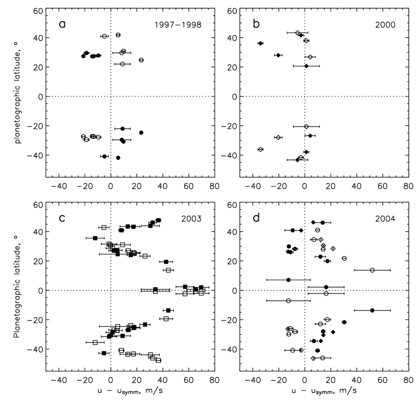
Figure 8.— Zonal wind speed relative to the symmetric fit displayed in Fig. 6 for different time periods: (a) 1997-98, from Karkoschka (1998) and Hammel et al. (2001), (b) 2000, from Hammel et al. (2001), (c) 2003, from Hammel et al. (2005), and (d) 2004, from this work, which includes highly accurate observations from tracking clouds over a 1-month period (shown as diamonds). Filled symbols are direct observations; open symbols are their reflections about the equator.

4. Temporal changes in cloud characteristics

4.1. Temporal changes in morphology

Analysis of Voyager observations by Rages et al. (1991) inferred the existence of a southern polar cap of relatively thick clouds at about the 1.2-1.3 bar level, increasing in optical depth from 0.7 at 22.5^∘S to 2.4 at 66.5^∘S. The bright cap was still prominent in 1994, but declined significantly between 1994 and 2002. This was documented by Rages et al. (2004), who interpreted the changed appearance as a decline in the optical depth of the methane cloud, placed between 1.26 and 2 bars, which resulted in better views of deeper cloud patterns at the 4-bar level. (Be aware that the abstract of that paper erroneously states that the changes in cloud properties occurred between 2 and 4 bars, where their model actually has no cloud.) In Paper II we show that the current near IR variations in brightness with latitude cannot be explained by changes in cloud properties in the 1.2-1.3 bar range, but must occur deeper in the atmosphere, perhaps at the 4-bar level suggested by Rages et al. (2004) as the source of the bright band features. Between our 2003 and 2004 imaging observations little further change occurred in the overall morphology of the cloud bands, but there were many changes in discrete cloud features (Figs. 2, 3, and 4). Looking forward, it is not reasonable to expect a permanent north south asymmetry to exist in the Uranus’ cloud structure. The decline of the brightness of the south polar cap makes the south closer to the north-south average I/F. Likewise the relatively dark, recently exposed to view, northern hemisphere might very well brighten. If the contrast is due to solar forcing, it is likely that the two hemispheres might be already near a maximum in contrast and have started to move toward contrast reversal.

4.2. Evolution of discrete features

Not all changes on Uranus proceed at the sedate pace one might expect from the stability of cloud features observed by Karkoschka (1998). On 12 August 2004, we saw significant changes in the brightness of discrete features within the span of an 0.3-1.5 hours. Examples are given in Fig. 9, which displays remapped image strips centered on 20^∘N, at times 10:02 UT, 11:20 UT, and 12:46 UT. Between the first and the second image, features within the left circular outline essentially disappeared. By the third image, no trace of a cloud feature can be seen within the circle, while features just outside the circle have brightened considerably. Since the brightening and dimming features are of similar size, the changes cannot be attributed to changes in seeing. A similar brightening can be seen within the far right circular outline between the second and third image. Within the large circular outline near the center of the figure there is another example of dramatic declines in cloud brightness. These rapidly evolving features share the characteristic that they are relatively small, have relatively low brightness, and do not reach high altitudes (they are not visible in K^′ images).

It is useful to consider what mechanisms might have time scales that are compatible with these rapid changes. Particles of 300$\mu$m radius, inferred by Carlson et al. (1988) for the deeper clouds on Uranus, have sedimentation times (time to fall a scale height) that range from $\sim$3 hours at 1 bar to $\sim$10 hours at 7 bars. However, particles moved below the condensation level of their parent vapors by descending atmospheric flow will see a sudden decrease in ambient relative humidity, resulting in relatively rapid evaporation. Particles of 300-$\mu$m radius reaching the 60% saturation level would evaporate $\sim$10 minutes near 1.3 bars and in $\sim$30 minutes near 7 bars. A vertically thin cloud layer can thus be changed drastically by relatively small vertical motions. A 1-km thick cloud at 1.2 bars, would only need to move downward about 3 km to drop the relative humidity to 80%, at which point 300-$\mu$m particles could evaporate within 20 min. At 1 m/s, that 3-km drop would take less than an hour. Once formed, clouds can also be dissipated by vertical and horizontal shear, on time scales of the order of 1/($du/dy$) and 1/($du/dz$) respectively. The time scale for dissipation by horizontal shear has a minimum of $\sim$13 hours, while time scale for dissipation by vertical shear is 1/2 hour to 3 hours, based on the Flaser et al. (1987) vertical wind shear estimates. Clearly, the key factor controlling the lifetimes of the cloud features is the dynamics that produces vertical motions.

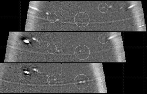
Figure 9.— Remapped 12 August 2004 H-band Keck images at 10:02 UT (bottom), 11:20 UT (middle), and 12:46 UT (top). Each strip covers latitudes from 5^∘N to 35^∘N. See text for description of evolving features within and near circular outlines. The arcing feature is the Epsilon ring. The second and third strips are offset longitudinally to compensate for the zonal drift rate at 20^∘N.

The striking group of high-altitude northern clouds appearing in the 12 July 2004 images (Fig. 3) provides an example of evolution in the larger features, although over a longer time interval. The K^′-bright cloud (136) at 26^∘N seems to be the origin of this large complex of cloud features extending over $\sim$40^∘ of longitude, which amounts to a distance of $\sim$30,000 km. There are five major features associated with this complex including feature 136. Just north of 136 is feature 137, which is at latitude 33.2^∘N. The measured drift rates for these features differ by 0.86$\pm$0.47^∘/h, and thus they do not travel together as fixed pattern. Among the other three components, 133 and 135 are both near 28.4^∘N and have slow drift rates between -0.34 and -0.48^∘/h. The final component (134) is displaced by 0.6^∘ to 27.8^∘N and has a somewhat faster drift rate of -0.55$\pm$0.2^∘/h.

The fact that discrete feature 136 is by far the brightest cloud feature in the K^′ image suggests that it is also the most energetic with respect to convective activity and may be the prime marker for a substantial dynamical feature that is responsible for creation of all these features. Looking ahead to the August 11-12 observations, there is another uniquely bright feature (209) which is at a similar latitude (25.25^∘N). That this is in fact the same feature identified as 136 in the July images is further confirmed by the continuity of the time varying longitude, assuming a constant drift rate, which has a best fit value of -3.01$\pm$0.01^∘ /day. Given the relative small dispersion in drift rates of the various other features associated with 136, one would expect to see them within 30^∘ of their original offsets from 136, after a month’s delay, presuming they lasted that long. As can be seen from Fig. 10, there are few features within 30^∘ of the original feature (labeled 209 in the upper panel).

Feature 136 itself actually declined significantly between 12 July and 12 August: in raw K^′ images its peak contrast dropped by a factor of 4.6 and its differential integrated brightness (Sromovsky et al. 2000), which is far less seeing dependent, dropped by a factor of 2.2. We estimated the size of this feature in deconvolved images. In both July and August it is about 5-6^∘ in longitudinal extent, but is so narrow in latitude that it can’t be resolved. A line scan through the feature has a full width at half maximum of $\sim$1.4^∘ , which corresponds to about 0.05^′′. Thus opacity differences and areal differences are both plausible contributors to the difference in contrast.

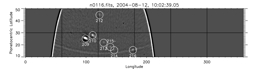
Figure 10.— Comparison of bright cloud features surrounding the 136/209 feature on 12 July (bottom) and 12 August (top) 2004.

5. Characterization of a long-lived circulation feature near 34^∘S.

5.1. Morphology of S34

Among the targets listed in Table 6 and displayed in Figs. 2-4, labels 301, 107, and 217 all refer to the same circulation feature, even though it does not appear at the same latitude during each time period. This is a significant feature, first noted by Sromovsky and Fry (2004) to have a long lifetime and unusual dynamics. For convenience we will hereafter refer to it as S34, named for its mean latitude. Target 301, the appearance of S34 in our 2003 images, is not listed in Table 6 because it could not be tracked long enough to yield an estimated wind speed error less than 60 m/s. However, its coordinates in 2003 images are listed in Table 9, along with coordinates in prior images where we believe this feature also appears. The case is quite strong that S34 has been present at least since the first detailed observations by Voyager in 1986, a time span of 18 years. Part of this case comes from continuity of latitudinal and longitudinal motions, which are described in subsequent sections. The other part comes from morphological evidence. Observations with complete longitude coverage (in 1986, 2000, 2003, 2004) generally show only a single prominent feature between 30^∘S and 40^∘S planetocentric latitudes. The appearance of the feature in HST and Voyager image samples from each of the time periods where it can be located are provided in Fig. 11. According to Paper II, the vertical location of this feature is generally mainly between 1.7 and 4 bars, and has a contrast of 20-30% in J and H bands. Scattering by overlying haze and methane cloud particles and Rayleigh scattering reduce contrast at shorter wavelengths.

Only recent Keck observations and Voyager 2 observations achieved sufficient spatial resolution to capture detailed morphological characteristics, which are compared in Fig. 12. In both 1986 and in 2004 the feature is seen to have two components, a long streaky northern component, which was thought to be a plume by Voyager investigators (Smith et al., 1986) and which extended over roughly 10-15^∘ of longitude, and a small more symmetric feature displaced 2.2-2.5^∘ to the south of the main feature. Intervening HST images by WFPC2 and NICMOS have detected this feature but have not been able to resolve the detailed 2-component morphology.

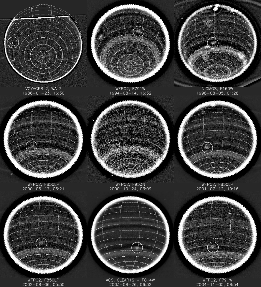
Figure 11.— S34 image samples from each of the periods where it has been identified. These are all high-pass filtered to enhance contrast, which is quite low in Voyager Wide-angle Orange and F953N WFPC2 images. See other figures for its appearance in recent Keck images.

Table 9Observations of S34.

Time	Relative	Planetocentric	Planetographic
yyyy-mm-dd hh:mm:ss	Julian Day	Latitude, ∘	(East) Longitude,∘             Source
1986-01-22 04:01:34	-6745.312	-34.00$\pm$0.20	288.60$\pm$0.5	Voyager WA Orange
1986-01-22 06:19:58	-6745.216	-34.30$\pm$0.20	285.70$\pm$0.3	Voyager WA Orange
1986-01-22 07:25:34	-6745.170	-34.65$\pm$0.20	284.80$\pm$0.3	Voyager WA Orange
1986-01-22 08:32:46	-6745.123	-34.70$\pm$0.20	-76.75$\pm$0.3	Voyager WA Orange
1986-01-22 18:35:58	-6744.705	-33.80$\pm$0.20	272.10$\pm$0.3	Voyager WA Orange
1986-01-22 19:28:46	-6744.668	-33.75$\pm$0.20	271.10$\pm$0.3	Voyager WA Orange
1986-01-22 23:38:22	-6744.495	-34.80$\pm$0.20	266.00$\pm$0.3	Voyager WA Orange
1986-01-22 00:21:34	-6744.465	-34.85$\pm$0.20	264.65$\pm$0.3	Voyager WA Orange
1986-01-23 02:23:10	-6744.380	-34.80$\pm$0.20	-97.30$\pm$0.3	Voyager WA Orange
1986-01-23 11:52:46	-6743.985	-33.60$\pm$0.20	252.70$\pm$0.3	Voyager WA Orange
1986-01-23 14:02:22	-6743.895	-34.10$\pm$0.20	249.50$\pm$0.3	Voyager WA Orange
1986-01-23 16:30:22	-6743.792	-34.25$\pm$0.20	245.40$\pm$0.4	Voyager WA Orange
1994-08-14 13:20:16	-3618.924	-33.60$\pm$0.50	56.60$\pm$2.0	HST WFPC2 F791W
1994-08-14 16:32:16	-3618.790	-34.30$\pm$0.50	54.60$\pm$2.0	HST WFPC2 F791W
1998-08-05 01:28:40	-2167.418	-35.50$\pm$0.30	206.00$\pm$1.0	HST NICMOS F160W
2000-06-16 15:52:14	-1485.818	-35.25$\pm$0.50	105.30$\pm$2.0	HST WFPC2 F850LP
2000-06-17 06:21:14	-1485.215	-35.70$\pm$0.20	85.80$\pm$2.0	HST WFPC2 F850LP
2000-06-17 19:13:14	-1484.679	-36.50$\pm$0.30	71.00$\pm$3.0	HST WFPC2 F850LP
2000-06-18 00:03:14	-1484.477	-36.35$\pm$0.60	67.30$\pm$2.0	HST WFPC2 F850LP
2000-06-18 12:34:38	-1483.955	-36.70$\pm$1.00	49.00$\pm$2.0	s4 of de Pater et al. 2002
2000-10-24 03:09:13	-1356.348	-35.90$\pm$0.50	218.10$\pm$3.0	HST WFPC2 F953N
2001-06-26 10:00:14	-1111.063	-34.90$\pm$0.50	31.00$\pm$1.0	HST WFPC2 FQCH4N15
2001-07-12 04:49:14	-1095.279	-34.30$\pm$0.50	-12.40$\pm$1.0	HST WFPC2 F850LP
2001-07-12 19:16:14	-1094.677	-35.00$\pm$0.30	-27.40$\pm$1.0	HST WFPC2 F850LP
2001-07-13 13:02:14	-1093.936	-34.30$\pm$0.30	-45.60$\pm$0.5	HST WFPC2 F850LP
2002-08-05 11:58:16	-705.981	-32.00$\pm$0.30	48.50$\pm$0.5	HST WFPC2 F850LP
2002-08-05 12:34:16	-705.956	-32.40$\pm$0.40	47.00$\pm$0.5	HST WFPC2 F850LP
2002-08-06 05:30:16	-705.250	-32.50$\pm$0.40	33.60$\pm$0.5	HST WFPC2 F850LP
2002-08-06 05:53:16	-705.234	-32.40$\pm$0.40	32.20$\pm$0.5	HST WFPC2 F850LP
2003-07-12 17:37:37	-364.745	-35.60$\pm$0.30	22.81$\pm$1.0	HST ACS F775W
2003-08-15 12:22:51	-330.964	-35.90$\pm$0.30	35.80$\pm$0.6	Keck NIRC2 H
2003-08-26 06:32:26	-320.207	-35.50$\pm$0.30	58.00$\pm$0.5	HST ACS F814W
2003-08-30 11:23:02	-316.005	-36.30$\pm$0.50	288.60$\pm$1.5	HST ACS F814W
2004-07-11 11:30:32	0.000	-33.35$\pm$0.20	280.59$\pm$1.0	Keck NIRC2 H
2004-07-12 15:27:37	1.165	-33.40$\pm$0.20	251.60$\pm$1.0	Keck NIRC2 H
2004-08-12 12:46:22	32.053	-33.20$\pm$0.20	171.90$\pm$0.6	Keck NIRC2 H
2004-11-05 08:54:16	116.891	-33.00$\pm$0.40	212.50$\pm$0.8	HST WFPC2 791W

The origin of the 2-component morphology is unclear, although it does bear some resemblance to bright cloud features associated with Great Dark Spots on Neptune (Sromovsky et al., 1993; 2002). According to Stratman et al. (2001), bright clouds can be generated by vortices in a manner analogous to the formation of orographic clouds. These formations can be displaced from the center of the vortex, and travel along with it, rather than following local zonal wind profile. Thus we speculate that there may be a vortex circulation underpinning the two bright cloud elements that characterize S34, both of which may be orographic in nature. The vortex would probably have a latitudinal extent comparable to the latitude displacement between the two cloud elements. That would make it a little less than half the linear size of the DS2 vortex on Neptune (Sromovsky et al., 1993), and only about 1/6 the size of Neptune’s Great Dark Spot. It should be noted however that no oval dark spot could be seen in any Voyager image of the Uranus feature.

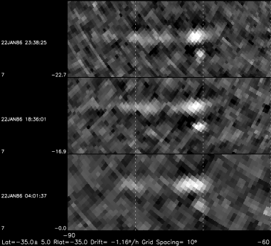
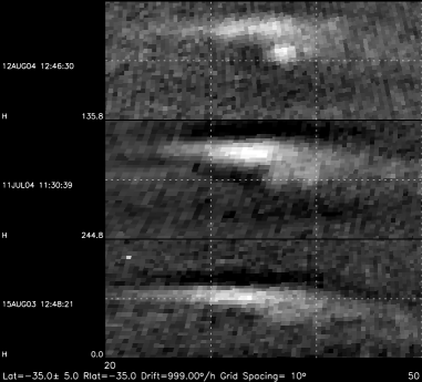
Figure 12.— Comparison of 34^∘S feature morphology in 1986 Voyager 2 wide-angle orange filtered images (left), and 2004 H filter NIRC2 Keck images. Both image groups are high-pass filtered to improve contrast. This is labeled as target 301, 107, and 217 in Figs. 2-4.

5.2. Motions of S34

In recent years, it has become very clear that S34 does not travel at a fixed drift rate and does not remain at a fixed latitude. In fact, both vary by substantial amounts, as illustrated in Fig. 13. S34 positions are given in Table 9 and S34 drift rates are given in Table 10 for time periods when observation frequency has permitted accurate drift rate determinations. These are the drift rates plotted in the lower panel of Fig. 13. The drift rate for 2003 was obtained by combining observations in Keck and HST images taken by the Advanced Camera for Surveys (ACS), acquired during observing program 9725 (E. Karkoschka, PI). At other times only a position observation was possible, sometimes with a very inaccurate drift rate determination. It is roughly the case that the longitudinal drift rate is a simple function of latitude that matches the zonal wind profile determined from tracking the 34^∘S feature and features at surrounding latitudes. This is illustrated in Fig. 14, compared to Karkoschka’s empirical fit of the zonal wind profile and to our fit to observations of S34.

Our empirical fits of the long-term variation in latitude ($\phi(t)$) and drift rate ($d\lambda(t)/dt$) of S34 make two assumptions: (1) there is a linear shear in the zonal wind and (2) the feature follows the zonal wind variation with latitude. The basic model equations that follow from these assumptions are these:

$$\phi(t) = \phi_{0}+c\sin(2\pi(t-t_{0})/T)$$ (1)

$$\frac{d\lambda(t)}{dt} = d_{ref}+d_{1}[\phi(t)-\phi_{ref}]$$ (2)

where $T$ is the period of variation, $c$ is the latitudinal amplitude, $\phi_{0}$ is the feature latitude at time $t_{0}$, $\phi_{ref}$ is the latitude at which the zonal wind drift rate is $d_{ref}$, and $d_{1}$ is the rate of change of drift rate with latitude. We used Eq. 2 to fit the drift rate results assuming a reference latitude of $\phi_{ref}=-34.16$^∘ and deriving $d_{ref}$=-26.9$\pm$0.5^∘/day and $d_{1}=$2.4$\pm$0.5^∘/day/^∘(lat.) by $\chi^{2}$ minimization. This fit is shown in Fig. 14 as a dot-dash line. We used Eq. 1 to fit the slow latitude variation; this is shown as the solid curve in the upper panel of Fig. 13. The dotted curves offset by $\pm$0.6^∘ of latitude illustrate the bounds of a short-period oscillation discussed below. The parameters of the latitude fit that minimize $\chi^{2}$ are $\phi_{0}$=-34.1$\pm$0.1^∘, $c=$2.1$\pm$0.2^∘, $t_{0}=$-45$\pm$10 days (for a time origin of 11:30:32 11 July 2004 UT), and $T=$1032$\pm$2 days. Plugging this latitude function into the best-fit version of Eq. 2 results in the dot-dash curve shown in the bottom panel of Fig. 13.

Figure 13.— Upper: 34S feature latitude vs time (symbols) and best-fit sinusoidal model fit (solid line), with dotted lines indicating expected variation due to inertial oscillations. The best-fit period is 1032 h and amplitude is 2.1^∘. Lower: 34S feature longitudinal drift rate versus time for periods when accurate rates were determined (symbols). The dashed curve is obtained from a fit of drift rate versus latitude with input from the above latitude versus time fit.

Table 10Determinations of zonal drift rates for S34.

	relative		longitudinal
mean time	timea, days	$<$latitude$>^{b}$,∘	drift ratec, ∘/day	data source
1986-01-22 21:06:06	-6744.600	-34.25$\pm$0.10	-27.43$\pm$0.20	Voyager WA Orange
2000-06-17 10:22:29	-1485.047	-35.95$\pm$0.30	-29.36$\pm$1.14	HST WFPC2 F850LP
2001-07-04 14:38:14	-1102.870	-34.62$\pm$0.50	-25.52$\pm$0.04	HST WFPC2 F850LP
2002-08-05 20:59:01	-705.605	-32.30$\pm$0.30	-21.20$\pm$0.65	HST WFPC2 F850LP
2003-08-13 11:58:58	-332.980	-35.82$\pm$0.21	-31.52$\pm$0.03	Keck + HST ACS
2004-07-22 13:14:50	11.072	-33.32$\pm$0.50	-25.87$\pm$0.02	Keck NIRC2 H

^aTime is measured from 11:30:32 on 11 July 2004.
^bPlanetocentric latitude averaged about the mean time.
^cRate of change of east (planetographic) longitude.

The fit shown in Fig. 13 illustrates that the oscillations in latitude and drift rate are not absolutely uniform, and deviate by more than the uncertainty in the measurements. The existence of a real short-term variation in latitude is confirmed by Voyager 2 observations, which provide the high latitudinal accuracy and temporal sampling needed to characterize it. The 1986 position measurements are plotted as a function of time in Fig. 15. The empirical fit (solid line) is a simple sine wave of amplitude 0.57$\pm$0.05^∘ and period 0.705$\pm$0.01 days (16.92 hours). Also shown in Fig. 15 is that a sinusoidal variation of this magnitude and frequency appears approximately consistent with the short-term variability seen in 2001, and possibly also with that seen in 2000 and 2002. A two-frequency oscillation is not unique to Uranus. Sromovsky et al. (2003) found a somewhat similar dynamical behavior in the 40^∘S Neptune feature known as the Scooter. However, for that feature the long oscillation period (110 days) was ten times smaller and the shorter oscillation period (22.5 days) was 30 times larger, and both latitude amplitudes were quite small (0.16^∘ and 0.315^∘ respectively). Neptune’s DS2 exhibited more substantial latitudinal oscillations with an amplitude of 2.4^∘, which is quite close to that of the 34^∘S feature on Uranus, though the 36-day period of the DS2 is much shorter (Sromovsky et al. 2003).

Figure 14.— Variation of eastward drift rate with latitude based on observations of the 34S feature.

Figure 15.— Short term latitude variation of the 34^∘S feature: Voyager results (top) and HST WFPC2 results (2000-2002). The phases are adjusted independently for the four cases.

Further constraints on the slow component of the 34^∘S oscillation can be obtained using longitudinal position coordinates, which can be useful even at times when temporal sampling does not permit determination of an accurate drift rate. The equation for the slow variation of longitude follows directly from the previous expressions for latitude and drift rate:

$$\lambda(t) = \lambda_{2}+d_{2}\times(t-t_{1})-c_{2}\cos(\frac{2\pi}{T}(t-t_{0})),$$ (3)

where

$$\lambda_{2} = \lambda_{1}+c_{2}\cos(\frac{2\pi}{T}(t_{1}-t_{0})),$$ (4)

$$d_{2} = d_{ref}+d_{1}[\phi_{0}-\phi_{ref}],$$ (5)

$$c_{2} = \frac{d_{1}cT}{2\pi},$$ (6)

where $\lambda_{1}$ is the longitude at time $t_{1}$, where $c$, $d_{1}$, and $\phi_{ref}$ are defined by Eqs. 1 and 2. Inserting into Eqs. 5 and 6 the coefficient values derived from fitting latitude vs time and drift rate vs latitude, we obtain the estimates $d_{2}$ = -26.756$\pm$0.5^∘, and $c_{2}$ = 827$\pm$80^∘. Since the estimated longitudinal excursion relative to a uniformly drifting longitude is two orders of magnitude greater than the $\sim$1-2^∘ accuracy with which feature longitude can be measured, these observations can provide very tight constraints on the form of the variation, provided temporal sampling is adequate to eliminate the 360^∘ multiple ambiguity. Unfortunately, for most time periods the ambiguity is not easily resolved.

Even allowing for the inherent longitude ambiguities, we were not able make Eq. 3 accurately fit observations of both longitude and latitude for the entire time period from 1986 to 2004 using a single period of sinusoidal variation. Nor were the expected coefficient values for $d_{2}$ and $c_{2}$ successful in providing more than a very crude fit even for the 2000-2004 time period when sampling is most dense. Sample fits with altered coefficients are provided in Fig. 16. These fit coefficients are summarized in Table 11, along with $\chi^{2}$ calculations for the more densely sampled 2000-2004 period, and compared with expected values quoted above. The $\chi^{2}$ computation includes latitude, longitude, and drift rate differences. The latitude models are derived from the longitude models by inverting Eq. 2. The fit with the 1032-day oscillation period provides the best match to latitudinal observations over the entire time period but the worst overall fit quality over the 2000-2004 time period. The intermediate period fit ($T=$1071 d) provides a relatively good match to longitudes, drift rates, and latitude observations between 1994 and 2004, with the exception of the earliest 2001 point, which can only be explained if the feature is misidentified. This is certainly possible since the imaging during this period covers only a small time interval that does not permit examination of all longitudes. The correct feature might very well have been on the dark side of Uranus at this time. The longer period fit ($T$= 1128 d) in Fig. 16 (and Table 11) is able to fit this observation reasonably well, as well as most of the other longitude observations, although several are well outside the uncertainties of observation, especially the first 2000 point, which is missed by nearly 100^∘. From that point forward this fit matches the most accurate drift rate observations quite well and does fairly well matching the latitude observations. At earlier times, however, latitude observations are quite inconsistent with this fit.

Table 11Model fits to slow variations in east longitude of S34.

osc.		osc.	osc.	linear	long.
period	$<$drift rate$>$	ampl.	time ref.a	time ref.a	offset	Fit quality
$T$ (days)	$d_{2}$ (∘/day)	$c_{2}$ (∘ )	$t_{0}$ (days)	$t_{1}$ (days)	$\lambda_{2}$ (∘)	$(\chi^{2})^{b}$	$(\chi^{2})^{c}$
1032	-27.044d	827	-45	-1094.7d	15.0d	55,826
1071	-25.996	840	+21	-1356.6	22.7	16,372	9,398c
1128	-26.975	892	-35	-1356.4	271.3	20,948

^aTime is measured from 11:30:32 on 11 July 2004.
^bComputed for 2000-2004 combining longitude, latitude, and drift-rate differences.
^cThis value is for 2000-2004 but excludes the earliest 2001 observation.
^dAdjusted for best fit; other parameters in this row are from the long-term latitude fit.

Figure 16.— Longitude of the 34^∘ S feature vs time relative to fixed drift rates, and latitude and drift rates versus time for models with periods of 1071 days (upper pair of figures) and 1128 (lower pair). Longitude models are shown as solid curves. Fit coefficients and $\chi^{2}$ calculations are given in Table 11. The latitude models (dashed lines) are derived from the longitude fits using an inverted form of Eq. 3. For latitude results the drift rate scale should be read as degrees centric. Dotted curves surrounding the latitude fits show the range of the short-period oscillation. Observations are plotted as circles. Longitude uncertainties are much smaller than the symbol size.

Even the best fit in Table 11 has a $\chi^{2}$ dominated by longitude differences, which have RMS values that are 20 times the expected errors. The differences between observations and these simple fitting functions are found to be more systematic than random. For example, the $\chi^{2}$ value for the longer period fit can be halved by adding a second modulation with a 740-day period and an 80^∘amplitude. It is also possible to get much more accurate fits by fitting smaller time spans.

The inescapable conclusion from attempts to fit longitude observations is that the motion cannot be accurately describe by a simple sinusoidal variation in longitude about a constant drift rate. It may be that the motion is sinusoidal with a slowly varying frequency, or that there are multiple frequencies present. A useful investigation of these issues is limited by large temporal gaps that introduce rotational ambiguities. Additional observations of S34 positions at a frequency of several times per year for the next five years or more would provide excellent constraints on the nature of this variation.

5.3. Interpretations of short-period oscillations of S34

The short-period oscillation of S34 has characteristics reasonably consistent with an inertial oscillation, which is a circular flow in which there is a balance between the Coriolis force and the centrifugal force, and other horizontal forces are negligible. The period of an inertial oscillation is given by

$$T_{\mathrm{in}}=T_{rot}/(2\sin\phi_{pg}),$$ (7)

where $T_{rot}$ is the rotational period at latitude $\phi_{pg}$ (Holton, 1972). This evaluates to 15.84 h (0.66 earth days) at a centric latitude of -34^∘, which is within 1.08 h of the best-fit period. The radius of curvature of an inertial oscillation is proportional to the speed of the flow and inversely proportional to the Coriolis parameter ($2\Omega\sin\phi_{\mathrm{pg}})$. Measured in angle instead of physical distance, the oscillation amplitude in longitude is thus expected to be larger by the ratio of the latitudinal radius of curvature to the radius of rotation at the latitude of interest, which evaluates to $1/\cos\phi$ for a spherical planet.

The longitude observations are somewhat too uncertain and too poorly distributed to provide much additional independent confirmation of the circular nature of the oscillation, although the results are reasonably consistent with such an oscillation. This is shown in Fig. 17, where latitudinal and longitudinal deviations are compared to model variations that are constrained to match the inertial period of 0.66 days, rather than the best-fit longitudinal period of 0.705 days. The longitudinal variations are deviations from a best fit constant drift rate computed from the 1986 Voyager observations. The solid line in the lower panel is the variation expected if the longitudinal motion simply followed the latitudinal shear in the zonal wind. The dotted curve is the variation expected from the inertial oscillation alone, in the absence of meridional wind shear. The dot-dash curve is the sum of the two contributions. The temporal sampling of the observations does not provide a very good constraint on the longitudinal model, but does seem to favor the shorter period computed for the ideal inertial oscillation, while the latitudinal variations clearly prefer a slightly longer period. The peak longitude variation about the mean drift longitude is also more consistent with the inertial model expectation, although the uncertainties are too large to make this compelling evidence that this is the dominant mechanism.

For an inertial oscillation, the instantaneous drift rate would be expected to vary by a significant amount when measured over short time intervals. The relative variation is given by the relation:

$$(d\lambda/dt)_{\mathrm{in}}=\frac{2\pi c_{\mathrm{in}}}{T_{\mathrm{in}}\sin\phi_{pg}}\sin(\frac{2\pi}{T_{\mathrm{in}}}t)$$ (8)

where $c_{\mathrm{in}}$ is the latitudinal amplitude of the inertial oscillation and $t$ is time measured from a zero of the latitudinal oscillation at which latitude is increasing. For $c_{\mathrm{in}}$ = 0.6^∘, $\phi$=-34^∘ ($\phi_{pg}$=-35.24^∘), and $T_{\mathrm{in}}$= 0.66 days, the amplitude of the drift rate modulation evaluates to 9.9^∘/day. This is somewhat surprising given that the amplitude of longitude modulation is only $\sim$1^∘. If this is sampled at positive and negative peaks, which are separated by only 0.33 days, it represents a drift rate deviation of $\sim$2^∘/0.33 days = 6^∘/day. When these deviations are sampled over a period of 0.99 days, the drift rate perturbation is reduced to a maximum of $\sim$2^∘/day. Since both negative and positive samples would be expected over two successive nights of observation, a significantly smaller perturbation would generally be expected. Nevertheless, some of the deviations in drift rate from the model fit shown in Fig. 13 could be due to imperfectly averaged inertial oscillations.

Figure 17.— Short term latitude and longitude variation of the 34^∘S feature based on Voyager results (top) and longitude variation relative to the best fit uniform drift rate. The solid line is the variation expected from the latitude shear only, the dotted line is the motion expected without latitudinal shear, and the dot-dash line is the sum of the two components.

5.4. Interpretation of slow oscillations of S34

Among well studied transverse atmospheric wave motions, only Rossby waves can yield long enough periods to match S34 observations. The Rossby wave arises from a gradient in planetary vorticity. It is a transverse wave that produces flow curvature that increases and decreases its relative vorticity to compensate for changes in planetary vorticity that result from deviations in latitude. This is the wave mode that is evident in the meandering jet stream on earth. In the northern hemisphere on earth, the phase speed is westward relative to the zonal flow. The period of the latitudinal oscillation is given by:

$$T=\frac{2\pi(k^{2}+m^{2}+f^{2}/gh)}{k\beta},$$ (9)

where the $k$ and $m$ are the zonal and meridional wavenumbers ($2\pi/$wavelength), $\beta=2\Omega\cos(\phi_{\mathrm{pg}})/a$ is the derivative of the Coriolis parameter with respect to latitude, $a$ is the local radius of curvature in the latitudinal direction, $g$ is the acceleration of gravity, and $h$ is an effective thickness parameter related to vertical stratification and involvement of vertical motions with the horizontal wave motions. This form, which ignores the small curvature of the zonal wind profile relative to $\beta$, is consistent with Pedlosky (1979). The last term in the numerator can be written in a number of ways, all dependent on the degree to which vertical motions participate in the wave motion. Here we use the expression that is the inverse square of the Rossby deformation radius. Two cases are illustrated in Fig. 18, both of which assume a meridional half-wavelength of 5^∘. The first case is pure barotropic, which has a maximum period of only about half what is observed for S34, even for a zonal wavenumber of unity (per circumference). The second case includes the vertical motion term, with the effective depth adjusted to produce a period of 1000 days at 34^∘S for the longest of the possible planetary wavelengths. The effective depth, which is only 0.65 km, cannot be interpreted as the true physical depth of the motion (see Pedlosky 1979). From this comparison, it is clear that a pure barotropic Rossby wave cannot be responsible for the long-period motion of S34, although a Rossby wave with coupled vertical motions is conceivable.

Figure 18.— Rossby wave periods for a wave confined to a 5^∘-wide latitude band as a function of zonal wave number (per circumference), for barotropic (dashed) conditions and for stratified conditions (solid) for an equivalent depth of 0.65 km. The observed period near 1000 days is best matched by the n=1 non-barotropic option.

6. Conclusions

Near-infrared adaptive optics imaging of Uranus by the Keck 2 telescope during 2003 and 2004 has revealed unprecedented numbers of discrete cloud features, which is partly due to improved adaptive optics performance and partly due to more of Uranus’ northern hemisphere becoming visible as the planet approaches its 2007 equinox. Increased cloud development might also play a role. Specific results of our investigation are based primarily on Keck observations we made in 2003 and 2004, but also on HST and Voyager observations. Our main conclusions are as follows:

1. Recent near IR adaptive optics imaging from the Keck telescope achieved angular resolutions near 0.05^′′, facilitating the detection of numerous discrete cloud features, which display a strong latitudinal variation in distribution and cloud characteristics, in reasonable accord with recent prior observations from the Keck telescope (de Pater et al. 2002, Hammel et al. 2005). The northern mid latitude features reach the highest altitudes and show the greatest K^′ contrast and sharpest horizontal structure, while equatorial features are dim and fuzzy. Features in the southern hemisphere were fewer in number, and none were seen south of a bright band near 45^∘S.

2. Measurement of cloud motions with estimated errors less than 50 m/s were obtained for 50 northern hemisphere features and 20 southern features. This has extended prior circulation measurements up to 60^∘N, where we found a maximum wind speed of 240$\pm$50 m/s. Prior results were limited to 46.4^∘ N (Hammel et al. 2005). We confirmed the presence of an asymmetry in the zonal circulation of Uranus, originally pointed out by Karkoschka (1998), and improved its characterization. We find that the asymmetry is mainly evident at mid latitudes where winds are more westward (prograde) in the southern hemisphere than in the northern hemisphere, with an average difference of $\sim$20 m/s.

3. There is no clear indication of sustained long-term change in wind speed between 1986 and 2004, although results of Hammel et al. (2001) based on 2001 HST and Keck observations are $\sim$10m/s less westward (less prograde) between 30^∘S and 45^∘S than earlier and later results, and results of Hammel et al. (2005) based on 2003 Keck observations are $\sim$30 m/s more westward (more prograde) between 20^∘N and 50^∘N than both 2000 and our 2004 results.

4. We found a large dispersion in lifetimes of discrete features that contrasts with Karkoschka’s characterization of features he observed with the HST NICMOS camera as relatively unchanged over a 100-day period (Karkoschka 1998). Some of the discrete cloud features we observed have relatively short lifetimes of $\sim$1 hour, some have disappeared within a month, while others have lasted at least one month, and S34 seems to have persisted for nearly two decades. The shortest lifetimes were observed for smaller low-contrast features that would not be visible in NICMOS images.

5. Based on detailed morphological similarities between high-resolution Voyager images in 1986 and Keck images in 2004, based on the continuity of latitudinal excursions as determined from HST and Keck imaging in 1994, 1998, 2000, 2001, 2002, 2003, and 2004, and from the fact that only a single feature of consistent morphology has appeared within the latitude band within which S34 is restricted, we believe that S34 has existed at least since 1986, which, if true, would make it the longest lived discrete feature on Uranus.

6. S34 oscillates in latitude between 32^∘S and 36.5^∘S, with a period of $\sim$1000 days, which may be a result of a non-barotropic Rossby wave. Its longitudinal drift rate varied between -20^∘E/day and -31^∘E/day in approximate accord with the latitudinal gradient in the zonal wind profile, exhibiting behavior similar to that of the DS2 feature observed on Neptune (Sromovsky et al., 1993). The Uranus feature also exhibits a superimposed much more rapid oscillation, with a latitudinal amplitude of 0.57^∘ and period 0.7 days, which is reasonably consistent with an inertial oscillation. The inertial oscillation has a longitudinal amplitude of $\sim$1^∘, which leads to a large variability in longitudinal drift rates measured over short time periods.

References

Acton, C. H. 1996. Ancillary data services of NASA’s Navigation and Ancillary Information Facility. Planet. Space Sci., 44, 65-70.

Allison, M. 1990. Planetary Waves in Jupiter’s Equatorial Atmosphere, Icarus 83, 282-307.

Allison, M., R. F. Beebe, B. J. Conrath, D. P. Hinson, A. P. Ingersoll 1991. Uranus atmospheric dynamics and circulation. In Uranus (J. T. Bergstralh, E. D. Miner, and M. S. Matthews, Eds.), pp 253-295, Univ. of Arizona Press, Tucson.

Baines, K. H., M. E. Mickelson, L. E. Larson, and D. W. Furguson 1995. The abundances of methane and ortho/para hydrogen in Uranus and Neptune: Implications for new laboratory 4-0 H₂ quadrupole line parameters. Icarus 114, 328-340.

Carlson, B. E., W. B. Rossow, and G. S. Orton 1988. Cloud Microphysics of the Giant Planets, J. Atmos. Sci. 45, 2066-2081.

Danielson, G.E, Kupferman, P.N., Johnson, T.V., Soderblom, L.A, 1981. Radiometric performance of the Voyager cameras. J. Geophys. Res. 86, 8683-8689.

de Pater, I., S. G. Gibbard, B. A. Macintosh, H. G. Roe, D. T. Gavel, and C. E. Max 2002. Keck Adaptive Optics Images of Uranus and Its Rings. Icarus 160, 359-374.

Flasar, F. M., B. J. Conrath, P. J. Gierasch, and J. A. Pirraglia 1987. Voyager Infrared Observations of Uranus’ Atmosphere: Thermal Structure and Dynamics. J. Geophs. Res. 92, 15011-15018.

Forsythe, K.J., M.S. Marley, H.B. Hammel, E. Karkoschka 1999. The Changing Face of Uranus, Bull Am. Astron. Soc. 31, 1153.

Friedson, J., and A. P. Ingersoll 1987. Seasonal Meridional Energy Balance and Thermal Structure of the Atmosphere of Uranus: A Radiative-Convective-Dynamical Model. Icarus 69, 135-156.

Hammel, H. B., K. Rages, G. W. Lockwood, E. Karkoschka, and I. de Pater 2001. New Measurements of the Winds of Uranus. Icarus 153, 229-235.

Hammel, H. B., I. de Pater, S. Gibbard, G. W. Lockwood, and K. Rages 2005. Uranus in 2003: Zonal Winds, Banded Structure, and Discrete Features. Icarus 175, 534-545.

Hanel, R. A., B. J. Conrath, F. M. Flasar, V. Kunde, W. Maguire, J. Pearl, J. Pirraglia, R. Samuelson, D. Cruikshank, D. Gautier, P. Gierasch, L. Horn, and P. Schulte 1986. Infrared observations of the Uranian system. Science 233, 70-74.

Holton, J. R. 1972. An Introduction to Dynamic Meteorology. Academic Press, New York, 319 pages.

Karkoschka, E. 1998. Clouds of High Contrast on Uranus. Science 111, 570-572.

Karkoschka, E. and M.G Tomasko 1998. Bright Discrete and Zonal Features on Uranus. Bull. Am. Astron. Soc. 30, 1056-1057.

Limaye, S. S., and L. A. Sromovsky 1991. Winds of Neptune: Voyager Observations of Cloud Motions. J. Geophys. Res. 96, 18941-18960.

Lindal, G. F., J. R. Lyons, D. N. Sweetnam, V. R. Eshelman, D. P. Hinson, and G. L. Tyler 1987. The atmosphere of Uranus: Results of radio occultation measurements with Voyager 2. J. Geophys. Res. 92, 14987-15001.

Pearl, J. C., and B. J. Conrath, R. A. Hanel, J. A. Pirraglia, and A. Coustenis 1990. The albedo, effective temperature, and energy balance of Uranus, as determined from Voyager IRIS data. Icarus 84, 12-28.

Pearl, J. C., and B. J. Conrath 1991. The Albedo, Effective Temperature, and Energy Balance of Neptune, as Determined from Voyager Data. J. Geophys. Res. 18921-18930.

Pedlosky, J., 1979. Geophysical Fluid Dynamics. Springer-Verlag, New York, 624 pages.

Rages, K.A., Pollack, J.B., Tomasko, M.G. Doose, L.R., 1991. Propertiesw of scatterers in the troposphere and lower stratospher of Uranus based on Voyager imaging data. Icarus 89, 359-376.

Rages, K. A., H. B. Hammel, and A. J. Friedson 2004. Evidence for temporal change at Uranus’ south pole. Icarus 172, 548-554.

Seidelmann, P. K., V. K. Abalakin, M. Bursa, M. E. Davies, C. de Bergh, J. H. Lieske, J. Oberst, J. L. Simon, E. M. Standish 2002. Report of the IAU/IAG Working Group on Cartographic Coordinates and Rotational Elements of the Planets and Satellites: 2000. Celestial Mechanics and Dynamical Astronomy 82, 83-110.

Smith, B.A., L.A. Soderblom, R.F. Beebe, D. Bliss, J.M. Boyce, A. Brahic, G.A. Briggs, R.H. Brown, S.A. Collins, A.F. Cook II, S.K. Croft, J.N. Cuzzi, G.E. Danielson, M.E. Davies, T.E. Dowling, D. Godfrey, C.J. Hansen, C. Harris, G.E. Hunt, A. P. Ingersoll, T.V. Johnson, R.J. Krauss, H. Masursky, D. Morrison, T. Owen, J.B. Plescia, J .B. Pollack, C.C. Porco, K. Rages, C. Sagan, E.M. Shoemaker, L.A. Sromovsky, C. Stoker, R.G. Strom, V.E. Suomi, S.P. Synnot, R.J. Terrile, P. Thomas, W.R. Thompson, and J. Veverka (1989). Voyager 2 in the Uranian System: Imaging Science Results. Science 233, 43-64.

Sromovsky, L. A., S. S. Limaye, and P. M. Fry 1993. Dynamics of Neptune’s Major Cloud Features. Icarus 105, 110-141.

Sromovsky, L. A., J. R. Spencer, K. H. Baines, and P. M. Fry 2000. Ground-Based Observations of Cloud Features on Uranus. Icarus 146, 307-311.

Sromovsky, L.A., P.M. Fry, K.H. Baines, S.S. Limaye, G.S. Orton, and T.E. Dowling 2001. Coordinated 1996 HST and IRTF Observations of Neptune and Triton I: Observations, Navigation, and Differential Deconvolution, Icarus 149, 416-434.

Sromovsky, L. A., V. E. Suomi, J. B. Pollack, R. J. Krauss, S. S. Limaye, T. Owen, H. E. Revercomb, and C. Sagan 1981. Implications of Titan’s north-south brightness asymmetry. Nature 292, 698-702.

Sromovsky, L.A., Fry, P.M., Baines, K.H., 2002. The unusual dynamics of northern dark spots on Neptune. Icarus 156, 16-36.

Sromovsky, L. A., and P. M. Fry 2004. Keck 2 AO Observations of Uranus in 2004. Bull. Am. Astron. Soc. 36, 1073.

Sromovsky, L. A., and P. M. Fry 2005. Cloud Structure on Uranus. Icarus, in preparation.

Stratman, P. W., A. P. Showman, T. E. Dowling, and L. A. Sromovsky 2001. EPIC Simulations of Bright Companions to Neptune’s Great Dark Spots. Icarus 151, 275-285.

Thompson, D., E. Egami, and M. Sawicki 2001. NIRC-2 The Keck Near-Infrared AO Camera Pre-ship testing. California Institute of Technology report available at http://www2.keck.hawaii.edu/ inst/nirc2/NIRC2Index.html.

Wallace, L., 1983. The Seasonal Variation of the Thermal Structure of the Atmosphere of Uranus. Icarus 54, 110-132.