A hybrid tree/finite-difference approach for
Heston-Hull-White type models

Abstract

We study a hybrid tree/finite-difference method which permits to obtain efficient and accurate European and American option prices in the Heston Hull-White and Heston Hull-White2d models. Moreover, as a by-product, we provide a new simulation scheme to be used for Monte Carlo evaluations. Numerical results show the reliability and the efficiency of the proposed methods.

Keywords: stochastic volatility; stochastic interest rate; tree methods; finite-difference; Monte Carlo; European and American options

1 Introduction

In this paper we consider the Heston-Hull-White model, which is a joint evolution for the equity value with a Heston-like stochastic volatility and a generalized Hull-White stochastic interest rate model which is consistent with the term structure of the interest rates. We consider a further situation where the dividend rate is stochastic, a case which is called here the “Heston Hull-White2d model” and can be of interest in the multi-currency (the dividend rate being interpreted as a further interest rate). We concern the problem of numerically pricing European and American options written on these models.

At the present time, the literature on this subject is quite poor and includes Fourier-Cosine methods, semi-closed approximations and finite-difference methods to price vanilla options. In [15], Grzelak and Oosterlee introduce two approximations of the non-affine models. The Fourier-Cosine method is then used on this approximating affine model. The authors remark that for accurate modeling of hybrid derivatives it is necessary to be able to describe a non-zero correlation between the processes driving the equity and the interest rate. This is possible in the approximations presented in their paper but only using approximated affine models. Haentjens and in’t Hout propose in [13] a finite-difference Alternating Direction Implicit (ADI) scheme for pricing European options solving the original three-dimensional Heston-Hull-White Partial Differential Equation (hereafter PDE). The Heston Hull-White2d model is treated using semi-closed approximations in the Foreign Exchange model [16].

In this paper, we generalize the hybrid tree/finite-difference approach that has been introduced for the Heston model in the paper [6]. In practice, this means to write down an algorithm to price European and American options by means of a backward induction that works following a finite-difference PDE method in the direction of the share process and following a recombining binomial tree method in the direction of the other random sources (volatility, interest rate and possibly dividend rate).

It is well known that there is a link between tree methods and finite-difference methods. The most remarkable benefits in using recombining binomial trees (let us stress the terms “recombining” and “binomial”: just two possible recombining jumps at each time-step for each component) are the simplicity of the implementation, the low computational costs and the efficiency of the output numerical results. In dimension 1, one can always build a recombining binomial tree (see e.g. Nelson and Ramaswamy [20]) but this is not the case in multidimensional problems. For example, in the standard (dimension 2) Heston model it is not possible to write down a recombining binomial approximating tree - roughly speaking, this follows from the fact that it is not possible to produce a function of the Heston components such that the associated Stochastic Differential Equation (SDE) has a diagonal diffusion coefficient. A binomial tree approximation for the standard Heston model has been proposed by Vellekoop and Nieuwenhuis in [22] but it is far from being recombining and, as shown in [6], it is problematic when the Feller condition is not satisfied. Finally, an approximation of the price coming from a numerical treatment of the (multidimensional) PDE can be very expensive, mainly to handle the 4-dimensional Heston-Hull-White2d model.

So, the idea underlying the approach developed in this paper is in some sense very simple: we apply the most efficient and easy to implement method whenever we can do it. In fact, wherever an efficient recombining binomial tree scheme can be settled (volatility, interest rate and possibly dividend rate), we use it. And where it cannot (share process), we use a standard (and efficient, being in dimension 1) numerical PDE approach. Hence we avoid to work with expensive (because non recombining and/or binomial) trees or with PDEs in high dimension. Moreover, for the Cox-Ingersoll-Ross (hereafter CIR) volatility component, we apply the recombining binomial tree method firstly introduced in [4], which theoretically converges and efficiently works in practice also when the Feller condition fails.

The description of the approximating processes coming from our hybrid tree/finite-difference approach, suggests a simple way to simulate paths from the Heston-Hull-White models. Therefore, we propose here also a new Monte Carlo algorithm for pricing options which seems to be a real alternative to the Monte Carlo method that makes use of the efficient simulations provided by Alfonsi [1].

Our approaches allow one to price options in the original Heston-Hull-White processes with non-zero correlations. Here, we consider the case of a non null correlation between the equity and the interest rate process, as well as between the equity and the stochastic volatility. Moreover, in the Heston-Hull-White2d model, we allow the dividend rate to be stochastic and correlated to the equity process. But it is worth noticing that other sets of correlations can surely be selected.

The paper is organized as follows. In Section 2 we introduce the Heston-Hull-White model. Then in Section 3 we construct a recombining binomial tree approximation for the pair given by the volatility and the interest rate process. Section 4 refers to the approximation of functions of the underlying asset price process by means of PDE arguments. In Section 5 we describe the hybrid tree/finite-difference scheme for the computation of American options. In Section 6 we see how to generalize the previous procedure in order to handle the Heston-Hull-White2d process. In Section 7 we show that our arguments can be used also to set-up simulations, to be applied to construct Monte Carlo algorithms. Finally, numerical results and comparisons with other existing methods are given in Section 8, showing the efficiency of the proposed methods in terms of the results and of the computational time costs.

2 The Heston-Hull-White model

The Heston Hull-White model concerns with cases where the volatility $V$ and the interest rate $r$ are assumed to be stochastic. The dynamics under the risk neutral measure of the share price $S$ and the volatility process $V$ are governed by the stochastic differential equation system

$$\frac{dS_{t}}{S_{t}}=(r_{t}-\eta)dt+\sqrt{V_{t}}\,dZ_{t},$$

$$dV_{t}=\kappa_{V}(\theta_{V}-V_{t})dt+\sigma_{V}\sqrt{V_{t}}\,dW^{1}_{t},$$

$$dr_{t}=\kappa_{r}(\theta_{r}(t)-r_{t})dt+\sigma_{r}dW^{2}_{t},$$

with initial data $S_{0}>0$, $V_{0}>0$ and $r_{0}>0$, where $Z$, $W^{1}$ and $W^{2}$ are suitable and possibly correlated Brownian motions. Recall that $V_{t}$ is a CIR process whereas $r_{t}$ is a generalized Ornstein-Uhlenbeck (hereafter OU) process: here $\theta_{r}$ is not constant but it is a deterministic function which is completely determined by the market values of the zero-coupon bonds (see [7]).

Let us fix the correlations among the Brownian motions. As observed in [15], the important correlations are between the pairs $(S,V)$ and $(S,r)$. So, we assume that $W=(W^{1},W^{2})$ is a standard Brownian motion in ${\mathbb{R}}^{2}$ and $Z$ is a Brownian motion in ${\mathbb{R}}$ which is correlated both with $W^{1}$ and $W^{2}$:

$$d\langle Z,W_{1}\rangle_{t}=\rho_{1}\,dt d\langle Z,W_{2}\rangle_{t}=\rho_{2}\,dt$$ and .

By passing to the logarithm $Y=\ln S$ in the first component and taking into account the above mentioned correlations, we reduce to the dynamics

$$dY_{t}=(r_{t}-\eta-\frac{1}{2}V_{t})dt+\sqrt{V_{t}}\,\big{(}\rho_{1}dW^{1}_{t}+\rho_{2}dW^{2}_{t}+\rho_{3}dW^{3}_{t}\big{)},\quad Y_{0}=\ln S_{0}\in{\mathbb{R}},$$

$$dV_{t}=\kappa_{V}(\theta_{V}-V_{t})dt+\sigma_{V}\sqrt{V_{t}}\,dW^{1}_{t},\quad V_{0}>0,$$

$$dr_{t}=\kappa_{r}(\theta_{r}(t)-r_{t})dt+\sigma_{r}dW^{2}_{t},\quad r_{0}>0,$$

where $W=(W^{1},W^{2},W^{3})$ is a standard Brownian motion in ${\mathbb{R}}^{3}$ and the correlation parameter $\rho_{3}$ is given by

$$\rho_{3}=\sqrt{1-\rho_{1}^{2}-\rho_{2}^{2}}\quad\mbox{with}\quad\rho_{1}^{2}+\rho_{2}^{2}<1.$$

As already done in [14], the process $r$ can be written in the following way:

$$r_{t}=\sigma_{r}X_{t}+\varphi_{t}$$ (2.1)

where

$$X_{t}=-\kappa_{r}\int_{0}^{t}X_{s}\,ds+\,W^{2}_{t}\quad\mbox{and}\quad\varphi_{t}=r_{0}e^{-\kappa_{r}t}+\kappa_{r}\int_{0}^{t}\theta_{r}(s)e^{-\kappa_{r}(t-s)}ds.$$ (2.2)

So, we can consider the triple $(Y,V,X)$, whose dynamics is given by

$$\begin{array}[]{ll}&dY_{t}=\mu_{Y}(V_{t},X_{t},t)dt+\sqrt{V_{t}}\,\big{(}\rho_{1}dW^{1}_{t}+\rho_{2}dW^{2}_{t}+\rho_{3}dW^{3}_{t}\big{)},\quad Y_{0}=\ln S_{0}\in{\mathbb{R}},\vskip 3.0pt plus 1.0pt minus 1.0pt\\ &dV_{t}=\mu_{V}(V_{t})dt+\sigma_{V}\sqrt{V_{t}}\,dW^{1}_{t},\quad V_{0}>0,\vskip 3.0pt plus 1.0pt minus 1.0pt\\ &dX_{t}=\mu_{X}(X_{t})dt+dW^{2}_{t},\quad X_{0}=0,\end{array}$$ (2.3)

where

$$\mu_{Y}(v,x,t)=\sigma_{r}x+\varphi_{t}-\eta-\frac{1}{2}\,v,$$ (2.4)

$$\mu_{V}(v)=\kappa_{V}(\theta_{V}-v),$$ (2.5)

$$\mu_{X}(x)=-\kappa_{r}x.$$ (2.6)

The purpose of this paper is to efficiently approximate the process $(Y,V,X)$ in order to numerically compute the price of options written on the share process $S$.

3 The recombining binomial tree for the pair $X$ and $V$

First of all, we consider an approximation for the pair $(V,X)$ on the time-interval $[0,T]$ by means of a $2$-dimensional computationally simple tree, that is by means of a Markov chain that runs over a $2$-dimensional recombining bivariate lattice (recombining binomial tree). In the usual case, as in the Cox-Ross-Rubinstein tree [10], at each time step the process can jump either on the nearest up-node or on the nearest down-node. Here, we consider the possibility of “multiple jumps” as introduced in Nelson and Ramaswamy [20]. Roughly speaking, the process can again jump upward or downward but the up/down jump nodes might not be the nearest ones: they are defined as the up/down positions at the next time-step whose associated transition probabilities better interpolate the theoretical expectation of the transition. As discussed in Nelson and Ramaswamy [20], this is the best way to construct an efficient tree for the approximation of one-dimensional diffusion processes, especially when the diffusion coefficient is not constant. Figure 1 shows an example of possible “multiple jumps” for the trees that approximate our processes $X$ and $V$, that we are going to describe.

In this section, we consider a discretization of the time-interval $[0,T]$ in $N$ subintervals $[nh,(n+1)h]$, $n=0,1,\ldots,N$, with $h=T/N$.

3.1 The tree for $X$

The construction of the recombining binomial tree for the process $X$ is quite standard, because here the diffusion coefficient is constant. For $n=0,1,\ldots,N$, consider the lattice for the process $X$

$$\mathcal{X}_{n}^{h}=\{x_{n,j}\}_{j=0,1,\ldots,n}\quad\mbox{with}\quad x_{n,j}=(2j-n)\sqrt{h}$$ (3.1)

(notice that $x_{0,0}=0=X_{0}$). For each fixed $x_{n,j}\in\mathcal{X}_{n}^{h}$, we define the “up” and “down” jump by means of $j_{u}^{h}(n,j)$ and $j_{d}^{h}(n,j)$ defined by

$$j_{u}^{h}(n,j)=\min\{j^{*}\,:\,j+1\leq j^{*}\leq n+1\mbox{ and }x_{n,j}+\mu_{X}(x_{n,j})h\leq x_{n+1,j^{*}}\},$$ (3.2)

$$j_{d}^{h}(n,j)=\max\{j^{*}\,:\,0\leq j^{*}\leq j\mbox{ and }x_{n,j}+\mu_{X}(x_{n,j})h\geq x_{n+1,j^{*}}\},$$ (3.3)

$\mu_{X}$ being the drift of the process $X$, see (2.6). As usual, one sets $j_{u}^{h}(n,j)=n+1$ if $\{j^{*}\,:\,j+1\leq j^{*}\leq n+1\mbox{ and }x_{n,j}+\mu_{X}(x_{n,j})h\leq x_{n+1,j^{*}}\}=\emptyset$ and $j_{d}^{h}(n,j)=0$ if $\{j^{*}\,:\,0\leq j^{*}\leq j\mbox{ and }x_{n,j}+\mu_{X}(x_{n,j})h\geq x_{n+1,j^{*}}\}=\emptyset$. Note that the up/down jumps in (3.2)-(3.3) might not be the nearest up/down positions in the lattice at time $n+1$. An example is given in Figure 1-left, where the lattice $\mathcal{X}_{n}^{h}$ is drawn and some possible instances of $x_{n,j}$, $x_{n+1,j_{d}^{h}(n,j)}$ and $x_{n+1,j_{u}^{h}(n,j)}$ are shown to exhibit as the tree can be visited.

The transition probabilities are defined in order to better interpolate the expected local transition: starting from the node $(n,j)$, the probability that the process jumps to $j_{u}^{h}(n,j)$ and $j_{d}^{h}(n,j)$ at time-step $n+1$ are set as

$$p^{X,h}_{u}(n,j)=0\vee\frac{\mu_{X}(x_{n,j})h+x_{n,j}-x_{n+1,j_{d}^{h}(n,j)}}{x_{n+1,j_{u}^{h}(n,j)}-x_{n+1,j_{d}^{h}(n,j)}}\wedge 1\quad\mbox{and}\quad p^{X,h}_{d}(n,j)=1-p^{X,h}_{u}(n,j)$$ (3.4)

respectively. This gives rise to a Markov chain $(\hat{X}^{h}_{n})_{n=0,\ldots,N}$ that weakly converges, as $h\to 0$, to the diffusion process $(X_{t})_{t\in[0,T]}$ and turns out to be a robust tree approximation for the OU process $X$.

3.2 The tree for $V$

For the CIR volatility process $V$, we consider a recombining binomial tree procedure that again follows the “multiple jumps” approach. In this case the recombining lattice is built by means of the transformation

$$f(V_{t})=\frac{2}{\sigma_{V}}\,\sqrt{V_{t}}.$$

This transformation is particularly important because $f(V_{t})$ turns out to be a diffusion process with unit diffusion coefficient, and this fact is useful in order to construct a recombining lattice. Many authors (see e.g. [17] or [23]) propose tree algorithms for $V_{t}$ by working on the transformed process $f(V_{t})$. The unpleasant fact is that now the drift of $f(V_{t})$ is very bad and is such that the approximating process converges only when the Feller condition holds: $2\kappa_{V}\theta_{V}\geq\sigma^{2}_{V}$. In order to overcome this fact, we use the approach in [4], that, roughly speaking, works as follows: the tree structure is built by using again $f$ (see next (3.5)) but the possible jumps and the transition probabilities are set on the dynamics of the original (and not transformed) CIR process $V_{t}$ (see next (3.6)-(3.7) and (3.8)). The main fact is that now the weak convergence on the path space is achieved for every values of $\kappa_{V},\theta_{V},\sigma_{V}>0$, so the Feller condition is not required. Details and comparisons with other tree existing methods to approximate the CIR process are given in [4].

For $n=0,1,\ldots,N$, consider the lattice

$$\mathcal{V}_{n}^{h}=\{v_{n,k}\}_{k=0,1,\ldots,n}\quad\mbox{with}\quad v_{n,k}=\Big{(}\sqrt{V_{0}}+\frac{\sigma_{V}}{2}(2k-n)\sqrt{h}\Big{)}^{2}\mathrm{1\!l}_{\sqrt{V_{0}}+\frac{\sigma}{2}(2k-n)\sqrt{h}>0}$$ (3.5)

(notice that $v_{0,0}=V_{0}$). For each fixed $v_{n,k}\in\mathcal{V}_{n}^{h}$, we define the “up” and “down” jump by means of

$$k_{u}^{h}(n,k)=\min\{k^{*}\,:\,k+1\leq k^{*}\leq n+1\mbox{ and }v_{n,k}+\mu_{V}(v_{n,k})h\leq v_{n+1,k^{*}}\},$$ (3.6)

$$k_{d}^{h}(n,k)=\max\{k^{*}\,:\,0\leq k^{*}\leq k\mbox{ and }v_{n,k}+\mu_{V}(v_{n,k})h\geq v_{n+1,k^{*}}\}$$ (3.7)

where the drift $\mu_{V}$ of $V$ is defined in (2.6) and with the understanding $k_{u}^{h}(n,k)=n+1$ if $\{k^{*}\,:\,k+1\leq k^{*}\leq n+1\mbox{ and }v_{n,k}+\mu_{V}(v_{n,k})h\leq v_{n+1,k^{*}}\}=\emptyset$ and $k_{d}^{h}(n,k)=0$ if $\{k^{*}\,:\,0\leq k^{*}\leq k\mbox{ and }v_{n,k}+\mu_{V}(v_{n,k})h\geq v_{n+1,k^{*}}\}=\emptyset$. By construction, the up/down jumps in (3.6)-(3.7) might not be the nearest up/down positions in the lattice at time $n+1$. In Figure 1-right we show an example of the lattice $\mathcal{V}_{n}^{h}$ together with some possible instances of the triple $(v_{n,k},v_{n+1,k_{d}^{h}(n,j)},v_{n+1,k_{u}^{h}(n,j)})$.

The transition probabilities are defined in order to better interpolate the expected local transition: starting from the node $(n,k)$ the probability that the process jumps to $k_{u}^{h}(n,k)$ and $k_{d}^{h}(n,k)$ at time-step $n+1$ are set as

$$p^{V,h}_{u}(n,k)=0\vee\frac{\mu_{V}(v_{n,k})h+v_{n,k}-v_{n+1,k_{d}^{h}(n,k)}}{v_{n+1,k_{u}^{h}(n,k)}-v_{n+1,k_{d}^{h}(n,k)}}\wedge 1\quad\mbox{and}\quad p^{V,h}_{d}(n,k)=1-p^{V,h}_{u}(n,k)$$ (3.8)

respectively. This gives rise to a Markov chain $(\hat{V}^{h}_{n})_{n=0,\ldots,N}$ that weakly converges, as $h\to 0$, to the diffusion process $(V_{t})_{t\in[0,T]}$ and turns out to be a robust tree approximation for the CIR process $V$ - details are given in [4].

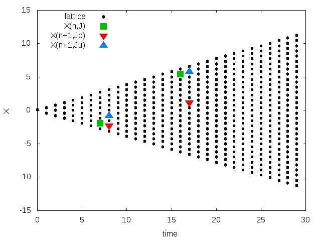
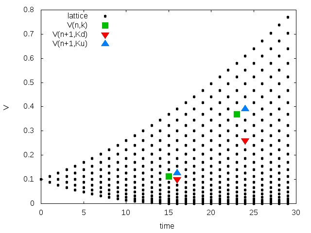
Figure 1: Example of a tree for $X$ on the left and of a tree for $V$ on the right.

3.3 The tree for the pair $(V,X)$

The tree procedure for the pair $(V,X)$ is set by joining the trees built for $V$ and for $X$. Namely, for $n=0,1,\ldots,N$, consider the lattice

$$\mathcal{V}_{n}^{h}\times\mathcal{X}_{n}^{h}=\{(v_{n,k},x_{n,j})\}_{k,j=0,1,\ldots,n}.$$ (3.9)

Starting from the node $(n,k,j)$, which corresponds to the position $(v_{n,k},x_{n,j})\in\mathcal{V}_{n}^{h}\times\mathcal{X}_{n}^{h}$, we define the four possible jump by setting the four nodes at time $n+1$ following the definitions (3.2)-(3.3) and (3.6)-(3.7):

$$\begin{array}[]{lcr}(n+1,k_{u}^{h}(n,k),j_{u}^{h}(n,j))&\hbox{with probability}&p^{h}_{uu}(n,k,j)=p^{V,h}_{u}(n,k)p^{X,h}_{u}(n,j),\vskip 3.0pt plus 1.0pt minus 1.0pt\\ (n+1,k_{u}^{h}(n,k),j_{d}^{h}(n,j))&\hbox{with probability}&p^{h}_{ud}(n,k,j)=p^{V,h}_{u}(n,k)p^{X,h}_{d}(n,j),\vskip 3.0pt plus 1.0pt minus 1.0pt\\ (n+1,k_{d}^{h}(n,k),j_{u}^{h}(n,j))&\hbox{with probability}&p^{h}_{du}(n,k,j)=p^{V,h}_{d}(n,k)p^{X,h}_{u}(n,j),\vskip 3.0pt plus 1.0pt minus 1.0pt\\ (n+1,k_{d}^{h}(n,k),j_{d}^{h}(n,j))&\hbox{with probability}&p^{h}_{dd}(n,k,j)=p^{V,h}_{d}(n,k)p^{X,h}_{d}(n,j),\end{array}$$ (3.10)

where the above probabilities $p^{V,h}_{u}(n,k)$, $p^{V,h}_{d}(n,k)$, $p^{X,h}_{u}(n,j)$ and $p^{X,h}_{d}(n,j)$ are defined in (3.8) and (3.4) respectively. The above factorization is due to the orthogonality of the noises driving the two processes. As a quite immediate consequence of standard results (see e.g. the techniques in [20]), one gets the following: the associated bivariate Markov chain $(\hat{V}^{h}_{n},\hat{X}^{h}_{n})_{n=0,\ldots,N}$ weakly converges to the diffusion pair $(V_{t},X_{t})_{t\in[0,T]}$ solution to

$$dV_{t}=\mu_{V}(V_{t})dt+\sigma_{V}\sqrt{V_{t}}\,dW^{1}_{t},\quad V_{0}>0,$$

$$dX_{t}=-\kappa_{r}X_{t}\,dt+\sigma_{r}\,dW^{2}_{t},\quad X_{0}=0.$$

Remark 3.1

In the case one is interested in introducing a correlation between the noises $W^{1}$ and $W^{2}$ driving the process $V$ and $X$ respectively, the joint tree can be constructed on the same lattice but the jump probabilities are no more of a product-type: the transition probabilities $p^{h}_{uu}(n,k,j)$, $p^{h}_{ud}(n,k,j)$, $p^{h}_{du}(n,k,j)$ and $p^{h}_{dd}(n,k,j)$ can be computed by matching (at the first order in $h$) the conditional mean and the conditional covariance between the continuous and the discrete processes of $V$ and $X$. More precisely, for both components the conditional mean is matched by construction (this is actually the main consequence of the definition of the multiple jumps). As for the conditional covariance, assuming that $d\langle W^{1},W^{2}\rangle_{t}=\alpha dt$, with $|\alpha|<1$, then one has $d\langle V,X\rangle_{t}=\alpha\sigma_{V}\sqrt{V_{t}}\,dt$. Therefore, the matching conditions lead to solving the following system:

$$\left\{\begin{array}[]{l}p^{h}_{uu}(n,k,j)+p^{h}_{ud}(n,k,j)=p^{V,h}_{u}(n,k)\vskip 3.0pt plus 1.0pt minus 1.0pt\\ p^{h}_{uu}(n,k,j)+p^{h}_{du}(n,k,j)=p^{X,h}_{u}(n,j)\vskip 3.0pt plus 1.0pt minus 1.0pt\\ p^{h}_{uu}(n,k,j)+p^{h}_{ud}(n,k,j)+p^{h}_{du}(n,k,j)+p^{h}_{dd}(n,k,j)=1\vskip 3.0pt plus 1.0pt minus 1.0pt\\ m^{h}_{uu}(n,k,j)p^{h}_{uu}(n,k,j)+m^{h}_{ud}(n,k,j)p^{h}_{ud}(n,k,j)+\vskip 3.0pt plus 1.0pt minus 1.0pt\\ \quad+m^{h}_{du}(n,k,j)p^{h}_{du}(n,k,j)+m^{h}_{dd}(n,k,j)p^{h}_{dd}(n,k,j)=\alpha\sigma_{V}\sqrt{v_{n,k}}\,h\end{array}\right.$$

where

$$\begin{array}[]{ll}&m^{h}_{uu}(n,k,j)=(v_{n+1,k^{h}_{u}(n,k)}-v_{n,k})(x_{n+1,j^{h}_{u}(n,j)}-x_{n,j}),\vskip 3.0pt plus 1.0pt minus 1.0pt\\ &m^{h}_{ud}(n,k,j)=(v_{n+1,k^{h}_{u}(n,k)}-v_{n,k})(x_{n+1,j^{h}_{d}(n,j)}-x_{n,j}),\vskip 3.0pt plus 1.0pt minus 1.0pt\\ &m^{h}_{du}(n,k,j)=(v_{n+1,k^{h}_{d}(n,k)}-v_{n,k})(x_{n+1,j^{h}_{u}(n,j)}-x_{n,j}),\vskip 3.0pt plus 1.0pt minus 1.0pt\\ &m^{h}_{dd}(n,k,j)=(v_{n+1,k^{h}_{d}(n,k)}-v_{n,k})(x_{n+1,j^{h}_{d}(n,j)}-x_{n,j}).\end{array}$$

This is done in [4] in a different context but the proof of the weak convergence on the path space is analogous - this can be done by standard arguments, as in [20] or [12].

4 Approximating the $Y$-component: the finite-difference approach

We go now back to (2.3), that is

$$\begin{array}[]{ll}&dY_{t}=\mu_{Y}(V_{t},X_{t},t)dt+\sqrt{V_{t}}\,\big{(}\rho_{1}dW^{1}_{t}+\rho_{2}dW^{2}_{t}+\rho_{3}dW^{3}_{t}\big{)},\quad Y_{0}=\ln S_{0},\vskip 3.0pt plus 1.0pt minus 1.0pt\\ &dV_{t}=\mu_{V}(V_{t})dt+\sigma_{V}\sqrt{V_{t}}\,dW^{1}_{t},\quad V_{0}>0,\vskip 3.0pt plus 1.0pt minus 1.0pt\\ &dX_{t}=\mu_{X}(X_{t})dt+dW^{2}_{t},\quad X_{0}=0,\end{array}$$

where $\mu_{Y}$, $\mu_{V}$ and $\mu_{X}$ are given in (2.4), (2.5) and (2.6) respectively. By isolating $\sqrt{V_{t}}dW^{1}_{t}$ in the second line and $dW^{2}_{t}$ in the third one, we obtain

$$dY_{t}=\frac{\rho_{1}}{\sigma_{V}}dV_{t}+\rho_{2}\sqrt{V_{t}}dX_{t}+\mu(V_{t},X_{t},t)dt+\rho_{3}\sqrt{V_{t}}\,dW^{3}_{t}$$ (4.1)

with

$$\begin{array}[]{rl}\mu(v,x,t)&=\mu_{Y}(v,x,t)-\frac{\rho_{1}}{\sigma_{V}}\mu_{V}(v)-\rho_{2}\sqrt{v}\,\mu_{X}(x)\vskip 3.0pt plus 1.0pt minus 1.0pt\\ &=\sigma_{r}x+\varphi_{t}-\eta-\frac{1}{2}\,v-\frac{\rho_{1}}{\sigma_{V}}\,\kappa_{V}(\theta_{V}-v)+\rho_{2}\kappa_{r}x\sqrt{v}.\end{array}$$ (4.2)

What we are going to do is mainly based on the fact that the noise $W^{3}$ is independent of the processes $V$ and $X$.

4.1 The approximating scheme for the triple $(Y,V,X)$

We consider an approximating process $Y^{h}$ for $Y$ turning out by freezing the coefficients in (4.1): we define $Y^{h}_{0}=Y_{0}$ and for $t\in[nh,(n+1)h]$ with $n=0,1,\ldots,N-1$ we set

$$Y^{h}_{t}= Y^{h}_{nh}+\frac{\rho_{1}}{\sigma_{V}}(V_{t}-V_{nh})+\rho_{2}\sqrt{V_{nh}}(X_{t}-X_{nh})+\mu(V_{nh},X_{nh},{nh})(t-nh)+\rho_{3}\sqrt{V_{nh}}\,(W^{3}_{t}-W^{3}_{nh}).$$

We consider now the approximating tree $(\hat{V}^{h}_{n},\hat{X}^{h}_{n})_{n\in\{0,\ldots,N\}}$ and we call $(\bar{V}^{h}_{t},\bar{X}^{h}_{t})_{t\in[0,T]}$ the associated time-continuous approximating process for the pair $(V,X)$, that is

$$\bar{V}^{h}_{t}=\hat{V}^{h}_{\lfloor t/h\rfloor}\quad\mbox{and}\quad\bar{X}^{h}_{t}=\hat{X}^{h}_{\lfloor t/h\rfloor}.$$

We then assume that the noise driving the pair $(\bar{V}^{h}_{t},\bar{X}^{h}_{t})_{t\in[0,T]}$ is independent of the Brownian motion $W^{3}$ and we insert this discretization for $(V,X)$ in the discretization scheme for $Y$. So, we obtain our final approximating process $\bar{Y}^{h}_{t}$ by setting $\bar{Y}^{h}_{0}=Y_{0}$ and for $t\in[nh,(n+1)h]$ with $n=0,1,\ldots,N-1$ then

$$\bar{Y}^{h}_{t}=Y^{h}_{nh}+\frac{\rho_{1}}{\sigma_{V}}(\bar{V}^{h}_{t}-\bar{V}^{h}_{nh})+\rho_{2}\sqrt{\bar{V}^{h}_{nh}}(\bar{X}^{h}_{t}-\bar{X}^{h}_{nh})+\mu(\bar{X}^{h}_{nh},\bar{V}^{h}_{nh},{nh})(t-nh)+\rho_{3}\sqrt{\bar{V}^{h}_{nh}}\,(W^{3}_{t}-W^{3}_{nh}).$$ (4.3)

Notice that if we set

$$\bar{Z}^{h}_{t}=\bar{Y}^{h}_{t}-\frac{\rho_{1}}{\sigma_{V}}(\bar{V}^{h}_{t}-\bar{V}^{h}_{nh})-\rho_{2}\sqrt{\bar{V}^{h}_{nh}}(\bar{X}^{h}_{t}-\bar{X}_{nh}),\quad t\in[nh,(n+1)h]$$ (4.4)

then we have

$$\begin{array}[]{l}d\bar{Z}^{h}_{t}=\mu(\bar{X}^{h}_{nh},\bar{V}^{h}_{nh},{nh})dt+\rho_{3}\sqrt{\bar{V}^{h}_{nh}}\,dW^{3}_{t},\quad t\in(nh,(n+1)h],\vskip 3.0pt plus 1.0pt minus 1.0pt\\ \bar{Z}^{h}_{nh}=\bar{Y}^{h}_{nh}\end{array}$$ (4.5)

that is $\bar{Z}^{h}$ solves a SDE with constant coefficients and at time $nh$ it starts from $\bar{Y}^{h}_{nh}$. Take now a function $f$: we are interested in approximating

$${\mathbb{E}}(f(Y_{(n+1)h})\mid Y_{nh}=y,V_{nh}=v,X_{nh}=x).$$

By using our scheme and the process $\bar{Z}^{h}$ in (4.4), we approximate it with the expectation done on the approximating processes, that is

$$\begin{array}[]{l}\displaystyle{\mathbb{E}}\big{(}f(\bar{Y}^{h}_{(n+1)h})\mid\bar{Y}^{h}_{nh}=y,\bar{V}^{h}_{nh}=v,\bar{X}^{h}_{nh}=x\big{)}\vskip 3.0pt plus 1.0pt minus 1.0pt\\ \displaystyle\qquad={\mathbb{E}}\big{(}f(\bar{Z}^{h}_{(n+1)h}+\frac{\rho_{1}}{\sigma_{V}}(\bar{V}^{h}_{(n+1)h}-\bar{V}^{h}_{nh})+\rho_{2}\sqrt{\bar{V}^{h}_{nh}}(\bar{X}^{h}_{(n+1)h}-\bar{X}^{h}_{nh}))\mid\bar{Z}^{h}_{nh}=y,\bar{V}^{h}_{nh}=v,\bar{X}^{h}_{nh}=x\big{)}.\end{array}$$

Since $(\bar{V}^{h},\bar{X}^{h})$ is independent of the Brownian noise $W^{3}$ driving $\bar{Z}^{h}$ in (4.4), we can write

$$\begin{array}[]{l}\displaystyle{\mathbb{E}}(f(\bar{Y}^{h}_{(n+1)h})\mid\bar{Y}^{h}_{nh}=y,\bar{V}^{h}_{nh}=v,\bar{X}^{h}_{nh}=x)\vskip 3.0pt plus 1.0pt minus 1.0pt\\ \qquad={\mathbb{E}}\Big{(}\Psi_{f}\Big{(}\frac{\rho_{1}}{\sigma_{V}}(\bar{V}^{h}_{(n+1)h}-v)+\rho_{2}\sqrt{v}(\bar{X}^{h}_{(n+1)h}-x);y,v,x\Big{)}\,\Big{|}\,\bar{V}^{h}_{nh}=v,\bar{X}^{h}_{nh}=x\Big{)},\end{array}$$ (4.6)

in which

$$\Psi_{f}(\xi;y,v,x)={\mathbb{E}}(f(\bar{Z}^{h}_{(n+1)h}+\xi)\mid\bar{Z}^{h}_{nh}=y,\bar{V}^{h}_{nh}=v,\bar{X}^{h}_{nh}=x).$$ (4.7)

Now, in order to compute the above quantity $\Psi_{f}(\xi)$, consider a generic function $g$ and set

$$u(s,z;v,x)={\mathbb{E}}(g(\bar{Z}^{h}_{(n+1)h})\mid\bar{Z}^{h}_{s}=z,\bar{V}^{h}_{s}=v,\bar{X}^{h}_{s}=x),\quad s\in[nh,(n+1)h].$$

By (4.5) and the Feynman-Kac representation formula we can state that, for every fixed $x\in{\mathbb{R}}$ and $v\geq 0$, the function $(s,z)\mapsto u(s,z;v,x)$ is the solution to

$$\left\{\begin{array}[]{l}\partial_{s}u+\mu(v,x,s)\partial_{z}u+\frac{1}{2}\rho_{3}^{2}v\partial^{2}_{z}u=0,\quad s\in[nh,(n+1)h),\ z\in{\mathbb{R}},\vskip 3.0pt plus 1.0pt minus 1.0pt\\ u((n+1)h,z;v,x)=g(z),\end{array}\right.$$ (4.8)

$\mu$ being given in (4.2). In order to solve the PDE problem (4.8), we use a finite-difference approach.

4.2 Finite-differences

At each time step $n$ we numerically solve (4.8) at time $s=nh$ by applying finite-difference techniques.

We fix a grid on the $y$-axis $\mathcal{Y}_{M}=\{y_{i}=Y_{0}+i\Delta y\}_{i\in\mathcal{J}_{M}}$, with $\mathcal{J}_{M}=\{-M,\ldots,M\}$ and $\Delta y=y_{i}-y_{i-1}$. For fixed $n$, $v\geq 0$ and $x\in{\mathbb{R}}$, we set $u^{n}_{i}=u(nh,y_{i};v,x)$ the discrete solution of (4.8) at time $nh$ on the point $y_{i}$ of the grid $\mathcal{Y}_{M}$ - for simplicity of notations, we do not stress in $u^{n}_{i}$ the dependence on $v$ and $x$ (from the coefficients of the PDE).

The finite difference method we are going to set is inspired from the one developed in [6]. But a main difference arises: here, we do not distinguish anymore between the diffusion dominant or reaction dominant case and we propose to apply a full implicit finite-difference approximation in time. In fact, the discrete solution $u^{n}$ to problem (4.8) at time $nh$ is computed in terms of the solution $u^{n+1}$ at time $(n+1)h$ by using the following finite-difference scheme:

$$\begin{array}[]{l}\displaystyle\frac{u^{n+1}_{i}-u^{n}_{i}}{h}+\mu(v,x,nh)\displaystyle\frac{u^{n}_{i+1}-u^{n}_{i-1}}{2\Delta y}+\frac{1}{2}\rho_{3}^{2}\ v\ \displaystyle\frac{u^{n}_{i+1}-2u^{n}_{i}+u^{n}_{i-1}}{\Delta y^{2}}=0.\end{array}$$ (4.9)

Of course, (4.9) has to be coupled with suitable numerical boundary relations. We assume that the boundary values are defined by the following Neumann-type conditions:

$$u^{n}_{-M-1}=u^{n}_{-M+1},\quad u^{n}_{M+1}=u^{n}_{M-1}.$$ (4.10)

Then, by applying the implicit finite-difference (4.9) coupled with the boundary conditions (4.10), we get the solution $u^{n}=(u^{n}_{-M},\ldots,u^{n}_{M})^{T}$ by solving the following linear system

$$A\,u^{n}=u^{n+1},$$ (4.11)

where $A=A(v,x)$ is the $(2M+1)\times(2M+1)$ tridiagonal real matrix given by

$$A=\left(\begin{array}[]{ccccc}1+2\beta&-2\beta&&&\\ -\beta+\alpha&1+2\beta&-\beta-\alpha&&\\ &\ddots&\ddots&\ddots&\\ &&-\beta+\alpha&1+2\beta&-\beta-\alpha\\ &&&-2\beta&1+2\beta\end{array}\right),$$ (4.12)

with

$$\alpha=\frac{h}{2\Delta y}\,\mu(v,x,nh)\quad\mbox{and}\quad\beta=\frac{h}{2\Delta y^{2}}\,\rho_{3}^{2}v,$$ (4.13)

$\mu$ being defined in (4.2). We stress that at each time step $n$, the quantities $v$ and $x$ are constant and known values (defined by the tree procedure for the pair $(V,X)$) and then $\alpha$ and $\beta$ are constant parameters too.

One can easily see that the implicit scheme (4.9) is unconditionally stable. Moreover, by applying standard results (Theorem 2.1 in [8] e.g.), the matrix $A$ is invertible for $\beta\neq|\alpha|$. Therefore, setting

$$\Pi(v,x)=A^{-1}(v,x),$$ (4.14)

the numerical solution to (4.8) on the grid $\mathcal{Y}_{M}$ through the above discretization procedure is given by

$$u(nh,y_{i};v,x)\simeq u^{n}_{i}=\sum_{\ell\in\mathcal{J}_{M}}\Pi_{i\ell}(v,x)g(z_{\ell}),\quad i\in\mathcal{J}_{M}.$$ (4.15)

Remark 4.1

Other numerical boundary conditions can surely be selected, for example the two boundary values $u^{n}_{-M}$ and $u^{n}_{M}$ may be a priori fixed by a known constant (this procedure typically appears in financial problems).

4.3 The scheme on the $Y$-component

We can now come back to our original problem, that is the computation of the function $\Psi_{f}(\xi;y,v,x)$ in (4.7) allowing one to numerically compute the expectation in (4.6).

We consider the approximating process $(\bar{Y}^{h},\bar{V}^{h},\bar{X}^{h})$ as described in Section 4.1. This means that the pair $(v,x)$ at time-step $n$ is located on the lattice $\mathcal{V}_{n}^{h}\times\mathcal{X}_{n}^{h}$: $v=v_{n,k}$ and $x=x_{n,j}$, for $0\leq k,j\leq n$. Then (4.15) gives the following approximation: for each $y_{i}\in\mathcal{Y}_{M}$,

$$\Psi_{f}\big{(}\xi;y_{i},v_{n,k},x_{n,j}\big{)}\simeq\sum_{\ell\in\mathcal{J}_{M}}\Pi_{i\ell}(v_{n,k},x_{n,j})f\big{(}y_{\ell}+\xi\big{)},\quad i\in\mathcal{J}_{M}.$$

Therefore, the expectation in (4.6) is computed on the approximating tree for $(V,X)$ by means of the above approximation:

$${\mathbb{E}}(f(\bar{Y}^{h}_{(n+1)h})\mid\bar{Y}^{h}_{nh}=y_{i},\bar{V}^{h}_{nh}=v_{n,k},\bar{X}^{h}_{nh}=x_{n,j})\simeq\!\!\!\sum_{a,b\in\{d,u\}}\sum_{\ell\in\mathcal{J}_{M}}\Pi_{i\ell}(v_{n,k},x_{n,j})\mathrm{T}_{n,k,j}f(\ell,a,b)p^{h}_{ab}(n,k,j)$$ (4.16)

where

$$\mathrm{T}_{n,k,j}f(\ell,a,b)=f\Big{(}y_{\ell}+\frac{\rho_{1}}{\sigma_{V}}(v_{n+1,k_{a}(n,k)}-v)+\rho_{2}\sqrt{v}(x_{n+1,j_{b}(n,j)}-x)\Big{)}$$

and the jump probabilities $p^{h}_{ab}(n,k,j)$ are given in (3.10) (or in Remark 3.1 if a correlation is assumed between the noises driving $V$ and $X$).

Similar arguments can be used in order to compute the conditional expectation in the left hand side of (4.16) when the function $f$ depends on the variables $v$ and $x$ also. Then one gets

$$\begin{array}[]{l}\displaystyle{\mathbb{E}}(f(\bar{Y}^{h}_{(n+1)h},\bar{V}^{h}_{(n+1)h},\bar{X}^{h}_{(n+1)h},)\mid\bar{Y}^{h}_{nh}=y_{i},\bar{V}^{h}_{nh}=v_{n,k},\bar{X}^{h}_{nh}=x_{n,j})\vskip 3.0pt plus 1.0pt minus 1.0pt\\ \qquad\simeq\displaystyle\sum_{a,b\in\{d,u\}}\sum_{\ell\in\mathcal{J}_{M}}\Pi_{i\ell}(v_{n,k},x_{n,j})\mathrm{T}_{n,k,j}f(\ell,a,b)p^{h}_{ab}(n,k,j)\end{array}$$ (4.17)

where

$$\begin{array}[]{l}\displaystyle\mathrm{T}_{n,k,j}f(\ell,a,b)=\vskip 3.0pt plus 1.0pt minus 1.0pt\\ \displaystyle\quad=f\Big{(}y_{\ell}+\frac{\rho_{1}}{\sigma_{V}}(v_{n+1,k_{a}(n,k)}-v_{n,k})+\rho_{2}\sqrt{v_{n,k}}(x_{n+1,j_{b}(n,j)}-x_{n,j}),v_{n+1,k_{a}(n,k)},x_{n+1,j_{b}(n,j)}\Big{)}.\end{array}$$ (4.18)

5 The algorithm for the pricing of American options

The natural application of the hybrid tree/finite-difference approach arises in the pricing of American options. Consider an American option with maturity $T$ and payoff function $(\Phi(S_{t}))_{t\in[0,T]}$. First of all, we consider the log-price process, so the obstacle will be given by

$$\Psi(Y_{t})=\Phi(e^{Y_{t}}),\quad t\in[0,T].$$

The price $P(t,y,v,x)$ of such an American option is given by (recall the relation between the interest rate $r$ and the process $X$: $r_{t}=\sigma_{r}X_{t}+\varphi_{t}$, see (2.1))

$$P(t,y,v,x)=\sup_{\tau\in\mathcal{T}_{t,T}}{\mathbb{E}}\Big{(}e^{-\int_{t}^{\tau}(\sigma_{r}X^{t,x}_{s}+\varphi_{s})ds}\Psi(Y^{t,y,v,x}_{\tau})\Big{)}$$

where $\mathcal{T}_{t,T}$ denotes the set of all stopping times taking values on $[t,T]$. Hereafter, $(Y^{t,y,v,x},V^{t,v},X^{t,x})$ denotes the solution of the SDE (2.3) starting at $(y,v,x)$ at time $t$.

The price at time $0$ of such an option is then approximated by a backward dynamic programming algorithm. Consider a discretization of the time interval $[0,T]$ into $N$ subintervals of length $h=T/N$: $[0,T]=\cup_{n=0}^{N-1}[nh,(n+1)h]$. Then $P(0,Y_{0},V_{0},X_{0})$ is numerically approximated through the quantity $P_{h}(0,Y_{0},V_{0},X_{0})$ which is iteratively defined as follows: for $(y,v,x)\in{\mathbb{R}}\times{\mathbb{R}}_{+}\times{\mathbb{R}}$,

$$\begin{cases}P_{h}(T,y,v,x)=\Psi(y)\quad\mbox{and as $n=N-1,\ldots,0$}\\ P_{h}(nh,y,v,x)=\max\Big{\{}\Psi(y),e^{-(\sigma_{r}x+\varphi_{nh})h}{\mathbb{E}}\Big{(}P_{h}\big{(}(n+1)h,Y^{nh,y,v,x}_{(n+1)h},V^{nh,v}_{(n+1)h},X^{nh,x}_{(n+1)h}\big{)}\Big{)}\Big{\}}.\end{cases}$$

From the financial point of view, this means to allow the exercise at the fixed dates $nh$, $n=0,\ldots,N$.

Consider now the discretization scheme $(\bar{Y}^{h},\bar{V}^{h},\bar{X}^{h})$ discussed in Section 4. We use the approximation (4.17) for the conditional expectations that have to be computed at each time step $n$. So, for every point $(y_{i},v_{n,k},x_{n,j})\in\mathcal{Y}_{M}\times\mathcal{V}_{n}^{h}\times\mathcal{X}_{n}^{h}$, (4.17) gives

$$\begin{array}[]{l}\displaystyle{\mathbb{E}}\Big{(}P_{h}\big{(}(n+1)h,Y_{(n+1)h}^{nh,y_{i},v_{n,k},x_{n,j}},V_{(n+1)h}^{nh,v_{n,k}},X_{(n+1)h}^{nh,x_{n,j}}\big{)}\Big{)}\\ \quad\simeq\displaystyle\sum_{a,b\in\{d,u\}}\sum_{\ell\in\mathcal{J}_{M}}\Pi_{i\ell}(v_{n,k},x_{n,j}){\mathcal{S}}_{n,k,j}P_{h}(\ell,a,b)\,p^{h}_{ab}(n,k,j)\end{array}$$ (5.1)

where ${\mathcal{S}}_{n,k,j}P_{h}$ denotes the operator in (4.18) applied to the function $P_{h}((n+1)h,\cdot)$, that is

$$\begin{array}[]{l}\displaystyle{\mathcal{S}}_{n,k,j}P_{h}(\ell,a,b)\\ \displaystyle=P_{h}\Big{(}(n+1)h,y_{\ell}+\frac{\rho_{1}}{\sigma_{V}}(v_{n+1,k_{a}(n,k)}-v_{n,k})+\rho_{2}\sqrt{v_{n,k}}(x_{n+1,j_{b}(n,j)}-x_{n,j}),v_{n+1,k_{a}(n,k)},x_{n+1,j_{b}(n,j)}\Big{)}.\end{array}$$ (5.2)

We finally summarize the backward induction giving our approximating algorithm. For $n=0,1,\ldots,N$, we define $\tilde{P}_{h}(nh,y,v,x)$ for $(y,v,x)\in\mathcal{Y}_{M}\times\mathcal{V}_{n}^{h}\times\mathcal{X}_{n}^{h}$ as follows:

$$\begin{cases}\tilde{P}_{h}(T,y_{i},v_{N,k},x_{N,j})=\Psi(y_{i})\quad\mbox{and as $n=N-1,\ldots,0$:}\\ \displaystyle\tilde{P}_{h}(nh,y_{i},v_{n,k},x_{n,j})=\max\Big{\{}\Psi(y_{i}),e^{-(\sigma_{r}x_{n,j}+\varphi_{nh})h}\times\\ \quad\qquad\qquad\qquad\qquad\qquad\qquad\qquad\times\displaystyle\sum_{a,b\in\{d,u\}}\sum_{\ell\in\mathcal{J}_{M}}\Pi_{i\ell}(v_{n,k},x_{n,j})p^{h}_{ab}(n,k,j){\mathcal{S}}_{n,k,j}\tilde{P}_{h}(\ell,a,b)\Big{\}}.\end{cases}$$ (5.3)

Notice that, by (5.2), the computation of ${\mathcal{S}}_{n,k,j}\tilde{P}_{h}(\ell,a,b)$ requires the knowledge of the function $y\mapsto\tilde{P}_{h}((n+1)h,y,v,x)$ in points $y$’s that do not necessarily belong to the grid $\mathcal{Y}_{M}$. Therefore, in practice we compute such a function by means of quadratic interpolations.

Remark 5.1

Let us stress that the r.h.s. of (5.1) can be read in two equivalents ways. First, the term

$$\sum_{\ell\in\mathcal{J}_{M}}\Pi_{i\ell}(v_{n,k},x_{n,j}){\mathcal{S}}_{n,k,j}P_{h}(\ell,a,b),\quad a,b\in\{d,u\},i\in\mathcal{Y}_{M},$$

is the numerical solution to the PDE (4.8) with final condition as in (5.2), so the r.h.s. of (5.1) is actually a weighted sum of the four solutions from each jump node $(a,b)\in\{d,u\}$ for the pair $(V,X)$, with weights given by the jump probabilities. But since the differential operator is linear in the Cauchy conditions, then one can first do the weighted sum of the final conditions, that is

$$\sum_{a,b\in\{d,u\}}{\mathcal{S}}_{n,k,j}P_{h}(\ell,a,b)\,p^{h}_{ab}(n,k,j),\quad\ell\in\mathcal{Y}_{M},$$

and then apply the matrix $\Pi(v_{n,k},x_{n,j})$, i.e. solve the PDE (4.8) just once, and this is of course computationally less expensive.

We can resume the main steps of our algorithm as follows.

• Preprocessing:

  • set the lattice $x_{n,j}$, $0\leq j\leq n\leq N$, for the process $X$ by using (3.1);

  • set the lattice $v_{n,k}$, $0\leq k\leq n\leq N$, for the process the $V$ by using (3.5);

  • merge the above lattices in a bivariate one $(v_{n,k},x_{n,j})$, $0\leq k,j\leq n\leq N$, by using (3.9);

  • compute the jump-nodes and the transition probabilities $p_{ab}$, $(a,b)\in\{d,u\}$, using (3.10);

  • set a mesh grid $y_{i}$, $i\in\mathcal{Y}_{M}$, for the solution of all the PDE’s.

• Step $N$: for each node $(v_{N,k},x_{N,j})$, $0\leq k,j\leq N$, compute the option prices at maturity for each $y_{i}$, $i\in\mathcal{Y}_{M}$, by using the payoff function.

• Step $n=N-1,\ldots 0$: for each $(v_{n,k},x_{n,j})$, $0\leq k,j\leq n$, compute the option prices for each $y_{i}$, $i\in\mathcal{Y}_{M}$, by solving PDE (4.8) through (4.15), with terminal condition given by the weighted sum of the values at nodes $(a,b)\in\{u,d\}$ which have been computed in the previous step - weight by using the transition probabilities $p_{ab}$ (recall Remark 5.1).

The theoretical proof of the convergence of our method is postponed to a further study. Although the ideas inspiring the method mainly come from [6], here the convergence problem has to be tackled differently. In fact, in [6] the numerical scheme is written through a matrix $\Pi$ which is stochastic, so one can link the scheme to a Markov chain that approximates the process $(Y,V,X)$ and use probabilistic methods (weak convergence) in order to study the convergence. But the scheme proposed here is purely numerical: the matrix $\Pi(v,x)=A^{-1}(v,x)$ in (4.14) is stochastic if and only if $\beta<|\alpha|$, so the link with Markov chains fails and the probabilistic weak convergence cannot be used anymore. So, here we restrict ourselves to the study of the behavior and the efficiency of the proposed approach from the numerical point of view, see next Section 8.

6 Generalization to the Heston-Hull-White2d model

The Heston-Hull-White2d model generalizes the previous model in the fact that the quantity $\eta$ is assumed to be stochastic and to follow a diffusion model itself. So, the underlying process is now $4$-dimensional and is given by: the share price $S$, the volatility process $V$, the interest rate $r$ and the continuous dividend rate $\eta$. Actually, here the process $\eta$ has not necessarily the meaning of a dividend rate, being for example a further interest rate process. In fact, the Heston-Hull-White2d model occurs in multi-currency models with short-rate interest rates, see e.g. [16].

Under the risk neutral measure, the dynamics are governed by the stochastic differential equation

$$\frac{dS_{t}}{S_{t}}=(r_{t}-\eta_{t})dt+\sqrt{V_{t}}\,dZ_{t},$$

$$dV_{t}=\kappa_{V}(\theta_{V}-V_{t})dt+\sigma_{V}\sqrt{V_{t}}\,dW^{1}_{t},$$

$$dr_{t}=\kappa_{r}(\theta_{r}(t)-r_{t})dt+\sigma_{r}dW^{2}_{t},$$

$$d\eta_{t}=\kappa_{\eta}(\theta_{\eta}(t)-\eta_{t})dt+\sigma_{\eta}dW^{3}_{t},$$

with initial data $S_{0},V_{0},r_{0},\eta_{0}>0$, where $Z$, $W^{1}$, $W^{2}$ and $W^{3}$ denote possibly correlated Brownian motions. Note that the process $\eta$ evolves as a generalized OU process: $\theta_{\eta}$ is a deterministic function of the time.

We consider non null correlations between the Brownian motions driving the pairs $(S,V)$, $(S,r)$ and $(S,\eta)$, that is

$$d\langle Z,W^{1}\rangle_{t}=\rho_{1}\,dt d\langle Z,W^{2}\rangle_{t}=\rho_{2}\,dt d\langle Z,W^{3}\rangle_{t}=\rho_{3}\,dt$$, , .

Correlations among the processes $V$, $r$ and $\eta$ can be surely inserted (see next Remark 6.1).

As done in Section 2, we take into account the transformations (2.1)-(2.2) for the generalized OU processes: we set

$$r_{t}=\sigma_{r}X^{r}_{t}+\varphi^{r}_{t}\quad\mbox{and}\quad\eta_{t}=\sigma_{\eta}X^{\eta}_{t}+\varphi^{\eta}_{t}$$ (6.1)

where

$$\begin{array}[]{ll}\displaystyle X^{r}_{t}=-\kappa_{r}\int_{0}^{t}X^{r}_{s}\,ds+\,W^{2}_{t},&\displaystyle\quad\varphi^{r}_{t}=r_{0}e^{-\kappa_{r}t}+\kappa_{r}\int_{0}^{t}\theta_{r}(s)e^{-\kappa_{r}(t-s)}ds,\vskip 3.0pt plus 1.0pt minus 1.0pt\\ X^{\eta}_{t}=-\kappa_{\eta}\int_{0}^{t}X^{\eta}_{s}\,ds+\,W^{3}_{t},&\displaystyle\quad\varphi^{\eta}_{t}=\eta_{0}e^{-\kappa_{\eta}t}+\kappa_{\eta}\int_{0}^{t}\theta_{\eta}(s)e^{-\kappa_{\eta}(t-s)}ds.\end{array}$$ (6.2)

So, by considering the $\log$-price process, we reduce to the $4$-dimensional process $(Y,V,X^{r},X^{\eta})$ whose dynamics is given by

$$\begin{array}[]{ll}&dY_{t}=\mu_{Y}(V_{t},X^{r}_{t},X^{\eta}_{t},t)dt+\sqrt{V_{t}}\,\big{(}\rho_{1}dW^{1}_{t}+\rho_{2}dW^{2}_{t}+\rho_{3}dW^{3}_{t}+\rho_{4}dW^{4}_{t}\big{)},\vskip 3.0pt plus 1.0pt minus 1.0pt\\ &dV_{t}=\mu_{V}(V_{t})dt+\sigma_{V}\sqrt{V_{t}}\,dW^{1}_{t},\vskip 3.0pt plus 1.0pt minus 1.0pt\\ &dX^{r}_{t}=\mu_{X^{r}}(X^{r}_{t})dt+dW^{2}_{t},\vskip 3.0pt plus 1.0pt minus 1.0pt\\ &dX^{\eta}_{t}=\mu_{X^{\eta}}(X^{\eta}_{t})dt+dW^{3}_{t},\vskip 3.0pt plus 1.0pt minus 1.0pt\\ &\mbox{with}\quad Y_{0}=\ln S_{0}\in{\mathbb{R}},\quad V_{0}>0,\quad X^{r}_{0}=0,\quad X^{\eta}_{0}=0\end{array}$$ (6.3)

where

$$\rho_{4}=\sqrt{1-\rho_{1}^{2}-\rho_{2}^{2}-\rho_{3}^{2}},\quad\mbox{with}\quad\rho_{1}^{2}+\rho_{2}^{2}+\rho_{3}^{2}<1,$$

$$\mu_{Y}(v,x_{1},x_{2},t)=\sigma_{r}x_{1}+\varphi^{r}_{t}-\sigma_{\eta}x_{2}-\varphi^{\eta}_{t}-\frac{1}{2}\,v,$$

$$\mu_{V}(v)=\kappa_{V}(\theta_{V}-v),\quad\mu_{X^{r}}(x)=-\kappa_{r}x,\quad\mu_{X^{\eta}}(x)=-\kappa_{\eta}x.$$

Starting from (6.3), we set-up an approximating procedure similar to the one developed in Section 3 and Section 4. In the following, we briefly describe how to extend such algorithms to the Heston-Hull-White2d model.

6.1 Approximation of $(V,X^{r},X^{\eta})$

Concerning the triple $(V,X^{r},X^{\eta})$, we build an approximating tree on ${\mathbb{R}}^{3}$ as follows:

• we apply the procedure in Section 3.1 to the process $X^{r}$;

• we apply the procedure in Section 3.1 to the process $X^{\eta}$;

• we apply the procedure in Section 3.2 to the process $V$.

We then get three approximating trees:

$$\hat{X}^{r,h} X^{r} \hat{X}^{\eta,h} X^{\eta} \hat{V}^{h} V$$ for ,  for ,  for .

Then, we use the null correlation between any two of $V$, $X^{r}$ and $X^{\eta}$: we concatenate the above trees in order to get a $3$-dimensional approximating tree $(\hat{V}^{h},\hat{X}^{r,h},\hat{X}^{\eta,h})$ for $(V,X^{r},X^{\eta})$ by introducing product-type jump probabilities. In other words, we generalize the probabilities in (3.10) for all the $2^{3}=8$ possible jumps.

Remark 6.1

One might include correlations between any two of the Brownian motions driving the processes $V$, $X^{r}$ and $X^{\eta}$. As described in Remark 3.1, the jump probabilities are no more of a product-type but they solve a linear system of equations that must include the matching of the local cross-moments up to order one in $h$.

6.2 The scheme on the $Y$-component and the approximating $4$-dimensional process

We repeat the reasonings in Section 4.1 in order to define an approximating time-continuous process $(\bar{Y}^{h},\bar{V}^{h},\bar{X}^{r,h},$ $\bar{X}^{\eta,h})$ for $(Y,V,X^{r},X^{\eta})$ - roughly speaking, it suffices to replace the one-dimensional process $X$ in Section 4.1 with the $2$-dimensional process $(X^{r},X^{\eta})$. So, we start from

$$dY_{t}=\frac{\rho_{1}}{\sigma_{V}}dV_{t}+\rho_{2}\sqrt{V_{t}}dX^{r}_{t}+\rho_{3}\sqrt{V_{t}}dX^{\eta}_{t}+\mu(V_{t},X^{r}_{t},X^{\eta}_{t},t)dt+\rho_{4}\sqrt{V_{t}}\,dW^{4}_{t}$$ (6.4)

with

$$\mu(v,x_{1},x_{2},t)=\mu_{Y}(v,x_{1},x_{2},t)-\frac{\rho_{1}}{\sigma_{V}}\mu_{V}(v)-\rho_{2}\sqrt{v}\,\mu_{X^{r}}(x_{1})-\rho_{3}\sqrt{v}\,\mu_{X^{\eta}}(x_{2}).$$ (6.5)

Then, we apply the finite-difference method in Section 4.2 and we obtain a final difference scheme given by

$$\Pi(v,x_{1},x_{2})=A^{-1}(v,x_{1},x_{2})$$

where, $\mu(\cdot)$ being defined in (6.5) and $A$ is given in (4.12) with

$$\alpha=\frac{h}{\Delta y}\,\mu(v,x_{1},x_{2},nh)\quad\mbox{and}\quad\beta=\frac{h}{2\Delta y^{2}}\,\rho_{4}^{2}v.$$ (6.6)

Finally, we extend the approximation scheme (4.17) to the case in which $X=(X^{r},X^{\eta})$ and the algorithm for the pricing of European or American options described in Section 5.

Remark 6.2

Let us briefly discuss the complexity of our algorithms. At each time step $n=0,\ldots,N=T/h$ one has to find the solution of a PDE on a grid with $2M+1$ points for each fixed values of

• case 1, Heston-Hull-White model: the pair $(v,x)\in\mathcal{V}^{h}_{n}\times\mathcal{X}^{h}_{n}$,

• case 2, Heston-Hull-White2d model: the triple $(v,x_{1},x_{2})\in\mathcal{V}^{h}_{n}\times\mathcal{X}^{h}_{n}\times\mathcal{X}^{h}_{n}$.

The cardinality of all these possible values in case $i$ is at most $n\times n^{i}$, $i=1,2$. For each case, the system of equations (4.11) with tridiagonal matrix (4.12), can be solved by an efficient form of Gaussian elimination requiring a linear cost of order $O(M)$. Therefore, the total cost of our approach is of order

$$\sum_{n=1}^{N}n^{i+1}\times(2M+1)=O(N^{i+2}\times M),\quad\mbox{case $i=1,2$}.$$

We notice that the use of a full finite-difference scheme could be more expensive for practical computations. Indeed, consider case 1 (Heston-Hull-White model). The solution of a $3$-dimensional problem by applying finite-differences in all three components leads to the inversion of a big band-matrix. To reduce the computational cost, the problem requires to apply appropriate techniques such as ADI (Alternating Direction Implicit) techniques, see [13] and references therein. Specifically, in [13] the authors propose an ADI approach to solve the Heston-Hull-White partial differential equation which needs a non-trivial implementation effort with a computational cost at least of order $O(M^{3})$ per time step, so the total cost is of order $O\big{(}N\times M^{3}\big{)}$ . Furthermore, as the dimension of the problem increases, it is not clear what happens if the problem is solved with a full finite-difference scheme. In case 2 (Heston-Hull-White2d model), one should solve a 4-dimensional problem, bringing to the inversion of a very big band-matrix. This would give a cost which is hard to be quantified, and possibly in such a case the costs of the two procedures are no longer comparable.

7 The hybrid Monte Carlo algorithm

The approximation we have set-up for the Heston-Hull-White processes can be used to construct a Monte Carlo algorithm. Let us see how one can simulate a single path by using the tree approximation and the standard Euler scheme for the $Y$-component. We call it “hybrid” because two different noise sources are considered: we simulate a continuous process in space (the component $Y$) starting from a discrete process in space (the 3-dimensional tree for $(V,X^{r},X^{\eta})$).

Concerning the Heston-Hull-White dynamics in Section 2, consider the triple $(Y,V,X)$ as in (2.3). Let $(\hat{V}^{h}_{n},\hat{X}^{h}_{n})_{n=0,1,\ldots,N}$ denote the Markov chain that approximates the pair $(V,X)$. We construct a sequence $(\hat{Y}_{n})_{n=0,1,\ldots,N}$ approximating $Y$ at times $n=0,1,\ldots,N$ by means of the Euler scheme defined in (4.3): we set $\hat{Y}^{h}_{0}=Y_{0}$ and for $t\in[nh,(n+1)h]$ with $n=0,1,\ldots,N-1$ then

$$\hat{Y}^{h}_{n+1}=\hat{Y}^{h}_{n}+\frac{\rho_{1}}{\sigma_{V}}(\hat{V}^{h}_{n+1}-\hat{V}^{h}_{n})+\rho_{2}\sqrt{\hat{V}^{h}_{n}}(\hat{X}^{h}_{n+1}-\hat{X}^{h}_{n})+\mu(\hat{V}^{h}_{n},\hat{X}^{h}_{n},{nh})h+\rho_{3}\sqrt{h\hat{V}^{h}_{n}}\,\Delta_{n+1},$$ (7.1)

where $\mu$ is defined in (4.2) and $\Delta_{1},\ldots,\Delta_{N}$ denote i.i.d. standard normal r.v.’s, independent of the noise driving the chain $(\hat{V},\hat{X})$. So, the simulation algorithm is very simple: at each time step $n\geq 1$, one let the pair $(V,X)$ evolve on the tree and simulate the process $Y$ at time $nh$ by using (7.1).

A similar algorithm can be considered to simulate the Heston-Hull-White2d dynamics in Section 6, that can be seen as a function of the triple $(Y,V,X^{r},X^{\eta})$ in (6.3). Here, we apply the Euler scheme to (6.4). So, let $(\hat{V}^{h}_{n},\hat{X}^{r,h}_{n},\hat{X}^{\eta,h}_{n})_{n=0,1,\ldots,N}$ denote the Markov chain approximating $(V,X^{r},X^{\eta})$, as described in Section 6.1. Starting from (6.4), we approximate the component $Y$ at times $nh$, $n=0,1,\ldots,N$, as follows: we set $\hat{Y}^{h}_{0}=Y_{0}$ and for $n=1,\ldots,N$, $n=0,1,\ldots,N-1$ then

$$\begin{array}[]{l}\displaystyle\hat{Y}^{h}_{n+1}=\hat{Y}^{h}_{n}+\frac{\rho_{1}}{\sigma_{V}}(\hat{V}^{h}_{n+1}-\hat{V}^{h}_{n})+\rho_{2}\sqrt{\hat{V}^{h}_{n}}(\hat{X}^{r,h}_{n+1}-\hat{X}^{r,h}_{n})+\rho_{3}\sqrt{\hat{V}^{h}_{n}}(\hat{X}^{\eta,h}_{n+1}-\hat{X}^{\eta,h}_{n})\vskip 3.0pt plus 1.0pt minus 1.0pt\\ \displaystyle\quad+\mu(\hat{V}^{h}_{n},\hat{X}^{r,h}_{n},\hat{X}^{\eta,h}_{n},nh)h+\rho_{4}\sqrt{h\hat{V}^{h}_{n}}\,\Delta_{n+1}\end{array}$$ (7.2)

where $\mu$ is defined in (6.5) and $\Delta_{1},\ldots,\Delta_{N}$ denote i.i.d. standard normal r.v.’s, independent of the noise driving the chain $(\hat{V}^{h},\hat{X}^{r,h},\hat{X}^{\eta,h})$. And again, the simulation algorithm is straightforward.

8 Numerical results

In this section we provide numerical results in order to asses the efficiency and the robustness of our hybrid numerical approach. We first consider test experiments for the Heston-Hull-White model for the computation of European, American and barrier options (Section 8.1) and, following Andersen [3], we study Vanilla options with large maturities when the Feller condition is not fulfilled (Section 8.2). Then we test European and American options in the Heston-Hull-White2d model (Section 8.3).

8.1 European, American and barrier options in the Heston-Hull-White model

In the European and American option contracts we are dealing with, we consider the following set of parameters:

• initial share price $S_{0}=100$, strike price $K=100$, maturity $T=1$, dividend rate $\eta=0.03$;

• initial interest rate $r_{0}=0.04$, speed of mean-reversion $\kappa_{r}=1$, interest rate volatility $\sigma_{r}=0.2$, time-varying long-term mean $\theta_{r}(t)$ which fits the theoretical bond prices to the yield curve observed on the market - to this purpose, we have chosen the interest rate curve given by $P_{r}(0,T)=e^{-0.04T}$;

• initial volatility $V_{0}=0.1$, long-mean $\theta_{V}=0.1$, speed of mean-reversion $\kappa_{V}=2$, volatility of volatility $\sigma_{V}=0.3$;

• varying correlations: for the pairs $(S,V)$, and $(S,r)$, we set $\rho_{1}=\rho_{SV}=-0.5$ and $\rho_{2}=\rho_{Sr}=-0.5,0,0.5$ respectively; no correlation is assumed to exist between $r$ and $V$.

We notice that, under the above requests, the Feller condition holds. We postpone to next Section 8.2 the analysis of cases in which the Feller condition is not fulfilled.

The numerical study of the hybrid tree/finite-difference method HTFD is split in two cases:

• HTFD1 refers to the (fixed) number of time steps $N_{t}=50$ and varying number of space steps $N_{S}=50,100,150,200$;

• HTFD2 refers to $N_{t}=N_{S}=50,100,150,200$.

Concerning the Monte Carlo method, we compare the results by using the hybrid simulation scheme in Section 7, that we call HMC. We also simulate paths by using the accurate third-order Alfonsi [1] discretization scheme for the CIR stochastic volatility process and by using an exact scheme for the interest rate. These simulating schemes are here called AMC. In both Monte Carlo methods, we consider varying number of time discretization steps $N_{t}=50,100,150,200$ and two cases for the number of Monte Carlo iterations:

• HMC1 and AMC1 refer to 50 000 iterations,

• HMC2 and AMC2 refer to 200 000 iterations.

In the European case, the benchmark value B-AMC is computed using the Alfonsi method with $300$ discretization time steps and the associated Monte Carlo estimator is computed with 1 million simulations. In the American case, in absence of reliable numerical methods, the benchmark values B-AMC-LS are obtained by the Longstaff-Schwartz [19] Monte Carlo algorithm with $50$ exercise dates, combined with the Alfonsi method with $300$ discretization time steps and 1 million iterations.

Table 1 reports both European call option prices and implied volatilities results. In Table 2 we provide American call option prices. Table 3 refers to the computational time cost (in seconds) of the different algorithms in the call European case.

The numerical results show that HTFD is accurate, reliable and efficient for pricing European and American options in the Heston-Hull-White model. Moreover, our hybrid Monte Carlo algorithm HMC appears to be competitive with AMC, that is the one from the accurate simulations by Alfonsi [1]: the numerical results are similar in term of precision and variance but HMC is definitely better from the computational times point of view. Additionally, because of its simplicity, HMC represents a real and interesting alternative to AMC. As a further evidence of the accuracy of our methods, in Figure 2 we study the shapes of implied volatility smiles across moneyness $\frac{K}{S_{0}}$ using HTFD1 with $N_{t}=50$ and $N_{S}=200$ and HMC1 with $N_{t}=50$, and we compare the graphs with the results from the benchmark.

In order to study the convergence behavior of our approach HTFD, we consider the convergence ratio proposed in [11], defined as

$$\mathrm{ratio}=\frac{P_{\frac{N}{2}}-P_{\frac{N}{4}}}{P_{N}-P_{\frac{N}{2}}},$$ (8.1)

where $P_{N}$ denotes here the approximated price obtained with $N=N_{t}$ number of time steps. Recall that $P_{N}=O(N^{-\alpha})$ means that $\mathrm{ratio}=2^{\alpha}$. For the sake of comparison with the numerical convergence speed studied in [6], we report ratios for American put options. We split the numerical study in two different cases: when the Feller condition holds and when it does not, the results being given in Table 4 and Table 5 respectively (details on the option parameters are given in the table captions). Both tables give evidence of the numerical convergence, but with some differences. In fact, under the Feller condition (Table 4), the numerical speed of convergence is definitely linear (this is not really surprising because tree methods are usually linear), whereas in the opposite case (Table 5) the behavior is approximately linear.

	$N_{S}$	HTFD1	HTFD2	B-AMC	HMC1	HMC2	AMC1	AMC2
$\rho_{Sr}=-0.5$	50	11.202744	11.202744	11.34$\pm$0.04	11.30$\pm$0.16	11.32$\pm$0.08	11.34$\pm$0.16	11.37$\pm$0.08
	100	11.319814	11.331040		11.41$\pm$0.16	11.38$\pm$0.08	11.31$\pm$0.16	11.36$\pm$0.08
	150	11.340665	11.349902		11.36$\pm$0.16	11.36$\pm$0.08	11.35$\pm$0.16	11.38$\pm$0.08
	200	11.346972	11.355772		11.34$\pm$0.16	11.37$\pm$0.08	11.44$\pm$0.16	11.39$\pm$0.08
$\rho_{Sr}=0$	50	12.526779	12.526779	12.77$\pm$0.04	12.66$\pm$0.18	12.69$\pm$0.09	12.68$\pm$0.18	12.79$\pm$0.09
	100	12.720651	12.705772		12.74$\pm$0.18	12.79$\pm$0.09	12.63$\pm$0.18	12.78$\pm$0.09
	150	12.754610	12.749526		12.74$\pm$0.18	12.79$\pm$0.09	12.68$\pm$0.18	12.81$\pm$0.09
	200	12.760365	12.766836		12.74$\pm$0.18	12.80$\pm$0.09	12.75$\pm$0.18	12.79$\pm$0.09
$\rho_{Sr}=0.5$	50	13.853193	13.853193	14.04$\pm$0.04	13.88$\pm$0.19	13.92$\pm$0.10	13.97$\pm$0.20	14.05$\pm$0.10
	100	14.011537	14.013063		13.91$\pm$0.19	14.01$\pm$0.10	13.89$\pm$0.19	14.06$\pm$0.10
	150	14.031598	14.038361		13.94$\pm$0.19	14.07$\pm$0.10	13.92$\pm$0.20	14.08$\pm$0.10
	200	14.038235	14.045612		13.99$\pm$0.19	14.07$\pm$0.10	13.90$\pm$0.19	14.06$\pm$0.10

	$N_{S}$	HTFD1	HTFD2	B-AMC	HMC1	HMC2	AMC1	AMC2
$\rho_{Sr}=-0.5$	50	0.279002	0.279002	0.282602	0.281649	0.282117	0.282602	0.283389
	100	0.282073	0.282367		0.284443	0.283681	0.281815	0.283127
	150	0.282620	0.282862		0.283034	0.283085	0.282865	0.283652
	200	0.282785	0.283016		0.282478	0.283408	0.285226	0.283914
$\rho_{Sr}=0$	50	0.313772	0.313772	0.320169	0.317398	0.317958	0.317802	0.320695
	100	0.318871	0.318480		0.319306	0.320650	0.316487	0.320432
	150	0.319764	0.319630		0.319063	0.320716	0.317802	0.321221
	200	0.319916	0.320086		0.319288	0.321009	0.319643	0.320695
$\rho_{Sr}=0.5$	50	0.348697	0.348697	0.353623	0.349329	0.350359	0.351777	0.353887
	100	0.352873	0.352913		0.350234	0.352954	0.349667	0.354151
	150	0.353402	0.353580		0.350960	0.354324	0.350458	0.354679
	200	0.353577	0.353771		0.352184	0.354545	0.349931	0.354151

Table 1: Prices (a) and Implied volatilities (b) of European call options. $S_{0}=100$, $K=100$, $T=1$, $r_{0}=0.04$, $\kappa_{r}=1$, $\sigma_{r}=0.2$, $\eta=0.03$, $V_{0}=0.1$, $\theta_{V}=0.1$, $\kappa_{V}=2$, $\sigma_{V}=0.3$, $\rho_{Sr}=-0.5,0,0.5$, $\rho_{SV}=-0.5$.

	$N_{S}$	HTFD1	HTFD2	B-AMC-LS
$\rho_{Sr}=-0.5$	50	12.090433	12.090433	12.22$\pm$0.01
	100	12.205014	12.212884
	150	12.224432	12.231392
	200	12.230288	12.237054
$\rho_{Sr}=0$	50	12.912708	12.912708	13.16$\pm$0.02
	100	13.119121	13.101073
	150	13.156492	13.149182
	200	13.162893	13.168602
$\rho_{Sr}=0.5$	50	13.944266	13.944266	14.15$\pm$0.02
	100	14.125059	14.122918
	150	14.146240	14.152060
	200	14.153288	14.160288

Table 2: Prices of American call options. $S_{0}=100$, $K=100$, $T=1$, $r_{0}=0.04$, $\kappa_{r}=1$, $\sigma_{r}=0.2$, $\eta=0.03$, $V_{0}=0.1$, $\theta_{V}=0.1$, $\kappa_{V}=2$, $\sigma_{V}=0.3$, $\rho_{Sr}=-0.5,0,0.5$, $\rho_{SV}=-0.5$.

$N_{S}$	HTFD1	HTDF2	B-AMC	HMC1	HMC2	AMC1	AMC
50	0.41	0.41	223.67	0.77	3.05	2.16	7.48
100	0.84	11.33		1.59	6.11	4.00	14.61
150	1.37	49.99		2.33	9.13	5.87	21.64
200	1.87	213.06		3.11	12.73	7.61	28.85

Table 3: Computational times (in seconds) for European call options.

Furthermore, we study the behavior of HTFD in the case of exotic options, namely for continuously monitored barrier options. We consider call up-and-out options, whose payoff is given by

$$(S_{T}-K)_{+}\mathrm{1\!l}_{\{S_{t}<H\,\forall\,t\leq T\}}.$$

In our numerical experiments, the up barrier is set at $H=130$ and we choose different values for $S_{0}=80,100,120$. Table 6 reports European call up-and-out option prices. In the barrier option case, we compare with a benchmark value, called B-AMC, computed by 2 millions iterations which use the Alfonsi AMC method with $9600$ discretization time steps. The numerical results confirm the reliability of HTFD for barrier options.

Figure 2: Moneyness vs implied volatility for European call options. $T=1$, $r_{0}=0.04$, $\kappa_{r}=1$, $\sigma_{r}=0.2$, $\eta=0.03$, $V_{0}=0.1$, $\theta_{V}=0.1$, $\kappa_{V}=2$, $\sigma_{V}=0.3$, $\rho_{Sr}=-0.5$, $\rho_{SV}=-0.5$.

K	$Nt$	$N$	Price	Ratio
80	25	50	21.494606
	50	100	21.534555
	100	200	21.553473	2.111762
	200	400	21.563911	1.812303
	400	800	21.569080	2.019428
100	25	50	12.607035
	50	100	12.749006
	100	200	12.815657	2.130053
	200	400	12.845050	2.267634
	400	800	12.859561	2.025489
120	25	50	21.444819
	50	100	21.539534
	100	200	21.572106	2.907912
	200	400	21.586338	2.288708
	400	800	21.592706	2.234825

Table 4: HTFD-ratio (8.1) for the price of American put options at final time $T=0.25$. $S_{0}=100$, $\eta=0.03$, $r_{0}=0.04$,$k_{r}=1$, $\sigma_{r}=0.2$, $V_{0}=0.1$, $k_{V}=2$, $\theta_{V}=0.1$, $\sigma_{V}=0.3$, $\rho_{SV}=-0.5$, $\rho_{Sr}=0.5$.

K	$Nt$	$N$	Price	Ratio
80	25	50	21.635830
	50	100	21.669504
	100	200	21.688879	1.738049
	200	400	21.700965	1.603169
	400	800	21.710373	1.284610
100	25	50	10.649104
	50	100	10.762867
	100	200	10.812709	2.282480
	200	400	10.835512	2.185787
	400	800	10.848349	1.776369
120	25	50	20.755654
	50	100	20.873859
	100	200	20.908825	3.380584
	200	400	20.919694	3.216994
	400	800	20.924295	2.362300

Table 5: HTFD-ratio (8.1) for the price of American put options at final time $T=0.25$. $S_{0}=100$, $\eta=0.03$, $r_{0}=0.04$,$k_{r}=1$, $\sigma_{r}=0.2$, $V_{0}=0.09$, $k_{V}=1$, $\theta_{V}=0.09$, $\sigma_{V}=1$, $\rho_{SV}=-0.3$, $\rho_{Sr}=0$.

	$N_{S}$	HTFD1	HTFD2	B-AMC
$S_{0}=80$	50	1.211544	1.211544
	100	1.251453	1.255849	1.282211$\pm 0.01$
	150	1.264327	1.270193
	200	1.269703	1.274332
$S_{0}=100$	50	1.819848	1.819848
	100	1.941320	1.916440	1.947565$\pm$0.01
	150	1.964666	1.930681
	200	1.974201	1.933482
$S_{0}=120$	50	0.697718	0.697718
	100	0.749116	0.725243	0.728431$\pm$0.01
	150	0.762224	0.726872
	200	0.766022	0.725139

Table 6: Prices of European call up-and-out options. Up barrier is $H=130$. $K=100$, , $T=1$, $r_{0}=0.04$, $\kappa_{r}=1$, $\sigma_{r}=0.2$, $\eta=0.03$, $V_{0}=0.1$, $\theta_{V}=0.1$, $\kappa_{V}=2$, $\sigma_{V}=0.3$, $\rho_{Sr}=-0.5$, $\rho_{SV}=-0.5$.

8.2 European options with large maturity in the Heston-Hull-White model

In order to verify the robustness of the proposed algorithms we consider experiments when the Feller condition is not fulfilled and with large maturities. We test here the cases I, II, III (reordered with respect to the maturity) proposed in Andersen [3] in order to price European call options. Moreover, we add the case IV with maturity $T=25$.

We consider the following values for the parameters of the model and for the maturity date:

• Case I: $V_{0}=0.09$, $\theta_{V}=0.09$, $\kappa_{V}=1$, $\sigma_{V}=1$, $\rho_{SV}=-0.3$, $T=5$;

• Case II: $V_{0}=0.04$, $\theta_{V}=0.04$, $\kappa_{V}=0.5$, $\sigma_{V}=1$, $\rho_{SV}=-0.9$, $T=10$.

• Case III: $V_{0}=0.04$, $\theta_{V}=0.04$, $\kappa_{V}=0.3$, $\sigma_{V}=0.9$, $\rho_{SV}=-0.5$, $T=15$.

• Case IV: $V_{0}=0.04$, $\theta_{V}=0.04$, $\kappa_{V}=0.3$, $\sigma_{V}=0.9$, $\rho_{SV}=-0.5$, $T=25$.

We take into account varying strikes $K=70,100,140$. No correlation is assumed to exist between $S$ and $r$, that is $\rho_{Sr}=0$, so we can compare the results with the semi closed-form analytic formula (SCF) for European call options which is available in [13]. We use in particular the implementation of the semi closed-form analytic formula provided in QuantLib [21]. Moreover in all cases the interest rate parameters, the initial share value and the dividend are the same of Section 8.1:

• $S_{0}=100$, $\eta=0.03$;

• $r_{0}=0.04$, $\kappa_{r}=1$, $\sigma_{r}=0.2$.

In Tables 7, 8, 9, 10 we provide European call option prices and implied volatility results. The numerical results suggest that large maturities bring to a slight loss of accuracy for both HTFD and HMC, even if each method provides a satisfactory approximation of the true option prices. It is worth noticing that for long maturities $T=5,15,25$ we have developed experiments with the same number of steps both in time ($N_{t}$) and space ($N_{S}$) as for $T=1$. So, the numerical experiments are not slower, and it is clear that one could achieve a better accuracy for larger values of $N_{t}$.

	$N_{S}$	HTFD1	HTFD2	SCF	HMC1	HMC2	AMC1	AMC2
$K=70$	50	37.054163	37.054163	37.491811	37.36$\pm$0.47	37.32$\pm$0.23	37.38$\pm 0.47$	37.31$\pm$0.23
	100	37.392491	37.395372		37.30$\pm$0.45	37.52$\pm$0.24	37.61$\pm 0.46$	37.61$\pm$0.24
	150	37.480467	37.521733		37.40$\pm$0.46	37.58$\pm$0.24	37.55$\pm 0.47$	37.58$\pm$0.24
	200	37.546885	37.570675		37.42$\pm$0.46	37.48$\pm$0.23	37.49$\pm 0.51$	37.60$\pm$0.24
$K=100$	50	23.997806	23.997806	24.706195	24.64$\pm$0.43	24.58$\pm$0.21	24.61$\pm 0.43$	24.54$\pm$0.21
	100	24.537750	24.540987		24.49$\pm$0.41	24.76$\pm$0.21	24.79$\pm 0.43$	24.81$\pm$0.22
	150	24.669356	24.684708		24.60$\pm$0.41	24.81$\pm$0.22	24.71$\pm 0.42$	24.78$\pm$0.22
	200	24.747161	24.766840		24.67$\pm$0.42	24.70$\pm$0.21	24.73$\pm 0.47$	24.82$\pm$0.22
$K=140$	50	13.672435	13.672435	14.324566	14.33$\pm$0.38	14.24$\pm$0.18	14.22$\pm 0.37$	14.17$\pm$0.18
	100	14.248533	14.205762		14.11$\pm$0.35	14.40$\pm$0.198	14.40$\pm 0.37$	14.40$\pm$0.19
	150	14.373163	14.318446		14.21$\pm$0.36	14.43$\pm$0.198	14.33$\pm 0.38$	14.40$\pm$0.19
	200	14.444183	14.404071		14.31$\pm$0.36	14.32$\pm$0.188	14.31$\pm 0.42$	14.42$\pm$0.20

	$N_{S}$	HTFD1	HTFD2	SCF	HMC1	HMC2	AMC1	AMC2
$K=70$	50	0.313372	0.313372	0.322137	0.319432	0.318614	0.319863	0.318541
	100	0.320152	0.320209		0.318384	0.322782	0.324521	0.324567
	150	0.321910	0.322734		0.320315	0.323861	0.323277	0.323956
	200	0.323236	0.323711		0.320737	0.321815	0.322027	0.324318
$K=100$	50	0.296912	0.296912	0.306954	0.306002	0.305124	0.30564	0.304539
	100	0.304563	0.304608		0.303947	0.307727	0.308148	0.308367
	150	0.306431	0.306649		0.305385	0.308440	0.307022	0.307959
	200	0.307536	0.307815		0.306431	0.306889	0.307262	0.308556
$K=140$	50	0.291198	0.291198	0.299737	0.299844	0.298690	0.298395	0.240057
	100	0.298743	0.298183		0.296939	0.300702	0.240301	0.239857
	150	0.300373	0.299657		0.298282	0.301138	0.299848	0.300773
	200	0.301301	0.300777		0.299533	0.299736	0.299505	0.301033

Table 7: Prices (a) and Implied volatilities (b) of European call options. $S_{0}=100$, $T=5$, $r_{0}=0.04$, $\kappa_{r}=1$, $\sigma_{r}=0.2$, $\eta=0.03$, $V_{0}=0.09$, $\theta_{V}=0.09$, $\kappa_{V}=1$, $\sigma_{V}=1$, $\rho_{Sr}=0$, $\rho_{SV}=-0.3$, $K=70,100,140$.

	$N_{S}$	HTFD1	HTFD2	SCF	HMC1	HMC2	AMC1	AMC2
$K=70$	50	33.702753	33.702753	34.101622	33.59$\pm$0.23	33.76$\pm$0.11	34.12$\pm 0.23$	34.09$\pm$0.11
	100	33.773407	34.120510		33.98$\pm$0.23	34.10$\pm$0.11	34.25$\pm 0.23$	34.10$\pm$0.11
	150	33.776196	33.818752		33.61$\pm$0.23	33.76$\pm$0.11	34.02$\pm 0.23$	34.11$\pm$0.11
	200	33.778268	33.944743		33.91$\pm$0.23	33.91$\pm$0.11	34.00$\pm 0.23$	34.10$\pm$0.11
$K=100$	50	22.540546	22.540546	23.140518	22.57$\pm$0.21	22.65$\pm$0.10	23.14$\pm 0.21$	23.09$\pm$0.11
	100	22.761622	23.076646		22.95$\pm$0.21	23.06$\pm$0.10	23.26$\pm 0.21$	23.12$\pm$0.11
	150	22.795766	22.857113		22.68$\pm$0.21	22.81$\pm$0.10	23.04$\pm 0.21$	23.09$\pm$0.11
	200	22.806087	22.978809		22.96$\pm$0.21	22.95$\pm$0.10	23.02$\pm 0.21$	23.13$\pm$0.11
$K=140$	50	13.335726	13.335726	13.755466	13.18$\pm$0.17	13.21$\pm$0.08	13.72$\pm 0.17$	13.68$\pm$0.09
	100	13.510432	13.726749		13.53$\pm$0.17	13.62$\pm$0.09	13.86$\pm 0.18$	13.72$\pm$0.09
	150	13.528322	13.553294		13.34$\pm$0.17	13.46$\pm$0.09	13.66$\pm 0.17$	13.73$\pm$0.09
	200	13.530288	13.639595		13.60$\pm$0.17	13.60$\pm$0.09	13.64$\pm 0.17$	13.76$\pm$0.09

	$N_{S}$	HTFD1	HTFD2	SCF	HMC1	HMC2	AMC1	AMC2
$K=70$	50	0.227844	0.227844	0.234811	0.225850	0.228795	0.235187	0.234676
	100	0.229082	0.235140		0.232714	0.234866	0.237332	0.234768
	150	0.229131	0.229876		0.226245	0.228809	0.233392	0.235042
	200	0.229167	0.232077		0.231443	0.231474	0.232965	0.234723
$K=100$	50	0.215548	0.215548	0.222789	0.215951	0.216908	0.222801	0.222156
	100	0.218214	0.222017		0.220435	0.221799	0.224184	0.222572
	150	0.218625	0.219366		0.217216	0.218739	0.221545	0.222656
	200	0.218750	0.220835		0.220583	0.220512	0.221377	0.222760
$K=140$	50	0.210662	0.210662	0.215154	0.209030	0.209283	0.214777	0.214386
	100	0.212532	0.214847		0.212764	0.213679	0.216253	0.214726
	150	0.212723	0.212991		0.210669	0.212018	0.214162	0.214846
	200	0.212744	0.213914		0.213460	0.213506	0.213908	0.215215

Table 8: Prices (a) and Implied volatilities (b) of European call options. $S_{0}=100$, $T=10$, $r_{0}=0.04$, $\kappa_{r}=1$, $\sigma_{r}=0.2$, $\eta=0.03$, $V_{0}=0.04$, $\theta_{V}=0.04$, $\kappa_{V}=0.5$, $\sigma_{V}=1$, $\rho_{Sr}=0$, $\rho_{SV}=-0.9$, $K=70,100,140$.

	$N_{S}$	HTFD1	HTFD2	SCF	HMC1	HMC2	AMC1	AMC2
$K=70$	50	32.872766	32.872766	33.182814	33.17$\pm$0.31	33.26$\pm$0.16	33.13$\pm$0.31	33.18$\pm$0.16
	100	33.041266	33.161213		33.10$\pm$0.30	33.29$\pm$0.15	33.18$\pm$0.31	33.19$\pm$0.15
	150	33.098186	33.159078		33.03$\pm$0.30	33.12$\pm$0.16	33.20$\pm$0.34	33.25$\pm$0.16
	200	33.150052	33.235555		33.02$\pm$0.29	33.11$\pm$0.15	33.12$\pm$0.33	33.35$\pm$0.15
$K=100$	50	24.738008	24.738008	25.183109	25.00$\pm$0.30	25.05$\pm$0.15	25.10$\pm$0.30	25.17$\pm$0.15
	100	24.979024	25.089961		24.96$\pm$0.29	25.18$\pm$0.15	25.20$\pm$0.30	25.20$\pm$0.15
	150	25.047214	25.150207		24.99$\pm$0.28	25.11$\pm$0.15	25.17$\pm$0.33	25.23$\pm$0.16
	200	25.103492	25.224136		24.97$\pm$0.28	25.09$\pm$0.15	25.07$\pm$0.31	25.30$\pm$0.15
$K=140$	50	17.522401	17.522401	17.851374	17.49$\pm$0.27	17.53$\pm$0.14	17.76$\pm$0.27	17.84$\pm$0.14
	100	17.702990	17.779408		17.51$\pm$0.26	17.74$\pm$0.14	17.85$\pm$0.28	17.86$\pm$0.15
	150	17.752550	17.858103		17.59$\pm$0.26	17.77$\pm$0.14	17.82$\pm$0.31	17.87$\pm$0.14
	200	17.800293	17.912261		17.59$\pm$0.25	17.75$\pm$0.13	17.73$\pm$0.29	17.93$\pm$0.14

	$N_{S}$	HTFD1	HTFD2	SCF	HMC1	HMC2	AMC1	AMC2
$K=70$	50	0.231761	0.231761	0.237013	0.236812	0.238369	0.236053	0.236928
	100	0.234617	0.236648		0.235577	0.238826	0.236974	0.237216
	150	0.235581	0.236612		0.234478	0.235946	0.237321	0.238081
	200	0.236459	0.237905		0.234214	0.235730	0.235877	0.239816
$K=100$	50	0.225390	0.225390	0.230837	0.228633	0.22926	0.229786	0.230708
	100	0.228336	0.229695		0.228045	0.230802	0.231012	0.231068
	150	0.229171	0.230433		0.228424	0.229935	0.230683	0.231375
	200	0.229861	0.231340		0.228236	0.229682	0.229474	0.232223
$K=140$	50	0.223601	0.223601	0.227024	0.223225	0.223688	0.226081	0.226894
	100	0.225479	0.226275		0.223424	0.225813	0.227054	0.227136
	150	0.225995	0.227094		0.224321	0.226215	0.226728	0.227195
	200	0.226492	0.227659		0.224316	0.225961	0.225781	0.227881

Table 9: Prices (a) and Implied volatilities (b) of European call options. $S_{0}=100$, $T=15$, $r_{0}=0.04$, $\kappa_{r}=1$, $\sigma_{r}=0.2$, $\eta=0.03$, $V_{0}=0.04$, $\theta_{V}=0.04$, $\kappa_{V}=0.3$, $\sigma_{V}=0.9$, $\rho_{Sr}=0$, $\rho_{SV}=-0.5$, $K=70,100,140$.

	$N_{S}$	HTFD1	HTFD2	SCF	HMC1	HMC2	AMC1	AMC2
$K=70$	50	28.772135	28.772135	28.969593	29.01$\pm$0.29	29.05$\pm$0.15	28.92$\pm$0.29	28.98$\pm$0.15
	100	28.890859	29.076376		29.06$\pm$0.34	29.00$\pm$0.15	28.99$\pm$0.29	28.97$\pm$0.15
	150	29.007171	29.225059		29.07$\pm$0.29	29.15$\pm$0.15	28.90$\pm$0.31	29.05$\pm$0.15
	200	29.125812	29.152251		29.05$\pm$0.31	28.91$\pm$0.15	28.95$\pm$0.29	29.01$\pm$0.14
$K=100$	50	23.947048	23.947048	24.255944	24.09$\pm$0.28	24.13$\pm$0.15	24.20$\pm$0.29	24.26$\pm$0.15
	100	24.107443	24.300298		24.22$\pm$0.33	24.19$\pm$0.155	24.27$\pm$0.28	24.25$\pm$0.15
	150	24.233382	24.462163		24.26$\pm$0.28	24.37$\pm$0.155	24.17$\pm$0.31	24.33$\pm$0.15
	200	24.356051	24.436578		24.32$\pm$0.31	24.20$\pm$0.145	24.22$\pm$0.28	24.31$\pm$0.14
$K=140$	50	19.352114	19.352114	19.601699	19.21$\pm$0.27	19.24$\pm$0.14	19.52$\pm$0.27	19.59$\pm$0.14
	100	19.459177	19.637550		19.39$\pm$0.32	19.39$\pm$0.14	19.62$\pm$0.27	19.59$\pm$0.14
	150	19.567765	19.778396		19.51$\pm$0.27	19.62$\pm$0.14	19.51$\pm$0.30	19.66$\pm$0.14
	200	19.692584	19.798050		19.60$\pm$0.30	19.53$\pm$0.14	19.55$\pm$0.27	19.65$\pm$0.13

	$N_{S}$	HTFD1	HTFD2	SCF	HMC1	HMC2	AMC1	AMC2
$K=70$	50	0.235972	0.235972	0.239830	0.240620	0.241466	0.238797	0.240057
	100	0.238291	0.241919		0.241551	0.240401	0.240301	0.239857
	150	0.240565	0.244831		0.241698	0.243433	0.239857	0.241365
	200	0.242887	0.243405		0.241403	0.238618	0.239442	0.239442
$K=100$	50	0.231127	0.231127	0.235633	0.233270	0.233862	0.234826	0.235633
	100	0.233464	0.236283		0.235133	0.234655	0.235771	0.235536
	150	0.235303	0.238656		0.235636	0.237270	0.234367	0.236650
	200	0.237099	0.238281		0.236537	0.234765	0.235096	0.236425
$K=140$	50	0.229635	0.229635	0.232641	0.227954	0.228325	0.231645	0.232511
	100	0.230923	0.233074		0.230084	0.230128	0.233016	0.232455
	150	0.2332231	0.234777		0.231504	0.232913	0.231583	0.233359
	200	0.2333739	0.235015		0.232634	0.231717	0.232046	0.233281

Table 10: Prices (a) and Implied volatilities (b) of European call options. $S_{0}=100$, $T=25$, $r_{0}=0.04$, $\kappa_{r}=1$, $\sigma_{r}=0.2$, $\eta=0.03$, $V_{0}=0.04$, $\theta_{V}=0.04$, $\kappa_{V}=0.3$, $\sigma_{V}=0.9$, $\rho_{Sr}=0$, $\rho_{SV}=-0.5$, $K=70,100,140$.

8.3 European and American options in the Heston-Hull-White2d model

In the European and American option contracts we are dealing with, we consider the following set of parameters:

• $S_{0}=100$, $K=100$, $T=1$;

• $r_{0}=0.04$, $\eta_{0}=0.03$, $\kappa_{r}=\kappa_{\eta}=1$, $\sigma_{r}=\sigma_{\eta}=0.2$;

• $V_{0}=0.1$, $\theta_{V}=0.1$, $\kappa_{V}=2$, $\sigma_{V}=0.3$;

• $\rho_{Sr}=-0.5,0,0.5$, $\rho_{SV}=-0.5$, $\rho_{S\eta}=-0.5,0.5$, $\rho_{Vr}=\rho_{V\eta}=\rho_{r\eta}=0$;

• $P_{r}(0,T)=e^{-0.04T}$, $P_{\eta}(0,T)=e^{-0.03T}.$

As before, the time-varying long-term means $\theta_{r}(t)$ and $\theta_{\eta}(t)$ fit the theoretical bond prices $P_{r}(0,T)$ and $P_{\eta}(0,T)$ to the yield curve observed on the market. We make this choice following the multi-currency models with short-rate interest rates in [16]. We consider here only the number of space steps $N_{S}=30,50,100$ because the cases $N_{S}=150,200$ need a too high computational time. Tables 11, 12 and 13 report European and American call option prices and implied volatilities. As before, the benchmark value for European options is computed using the Alfonsi B-AMC method with $300$ discretization time steps and the associated Monte Carlo estimator is computed with 1 million iterations. Concerning the benchmark B-AMC-LS for American options, it is computed by means of the Longstaff-Schwartz [19] Monte Carlo algorithm with $50$ exercise dates, combined with the Alfonsi method with $300$ discretization time steps and 1 million iterations. Table 14 refers to the computational time cost (in seconds) of the different algorithms in the call European case. In Figure 3 we compare the shapes of implied volatility smiles across moneyness $\frac{K}{S_{0}}$ using HTFD1 with $N_{t}=30$ and $N_{S}=100$ and HMC1 with $N_{t}=30$. The numerical results confirm the good numerical behavior of HTFD and HMC in the Heston-Hull-White2d model as well.

$\begin{array}[]{l}\rho_{SV}=-0.5,\\ \rho_{S\eta}=-0.5\end{array}$	$N_{S}$	HTFD1	HTFD2	B-AMC	HMC1	HMC2	AMC1	AMC2
$\rho_{Sr}=-0.5$	30	13.470572	13.470572	13.79 $\pm$ 0.04	13.82$\pm$0.20	13.74$\pm$0.10	13.83$\pm$0.20	13.79$\pm$0.10
	50	13.688842	13.671173		13.96$\pm$0.20	13.81$\pm$0.10	13.88$\pm$0.20	13.80$\pm$0.10
	100	13.790205	13.781519		14.00$\pm$0.20	13.80$\pm$0.10	13.68$\pm$0.20	13.73$\pm$0.10
$\rho_{Sr}=0$	30	14.736242	14.736242	15.04 $\pm$ 0.05	15.10$\pm$0.22	14.99$\pm$0.11	14.95$\pm$0.22	15.03$\pm$0.11
	50	14.958094	14.946029		15.23$\pm$0.22	15.04$\pm$0.11	14.98$\pm$0.22	15.01$\pm$0.11
	100	15.019204	15.032709		15.21$\pm$0.22	15.04$\pm$0.11	14.80$\pm$0.21	14.97$\pm$0.11
$\rho_{Sr}=0.5$	30	15.805046	15.805046	16.19 $\pm$ 0.03	16.13$\pm$0.23	16.06$\pm$0.11	16.04$\pm$0.23	16.17$\pm$0.12
	50	16.052315	16.032043		16.33$\pm$0.23	16.10$\pm$0.11	16.09$\pm$0.23	16.13$\pm$0.12
	100	16.155354	16.145308		16.24$\pm$0.23	16.19$\pm$0.12	15.93$\pm$0.23	16.12$\pm$0.12

$\begin{array}[]{l}\rho_{SV}=-0.5,\\ \rho_{S\eta}=-0.5\end{array}$	$N_{S}$	HTFD1	HTFD2	B-AMC	HMC1	HMC2	AMC1	AMC2
$\rho_{Sr}=-0.5$	30	0.338612	0.338612	0.347031	0.347724	0.345593	0.348085	0.347031
	50	0.344364	0.343898		0.351511	0.347675	0.349404	0.347294
	100	0.347036	0.346807		0.352510	0.347205	0.344131	0.345449
$\rho_{Sr}=0$	30	0.372004	0.372004	0.380033	0.381610	0.378689	0.377653	0.379769
	50	0.377867	0.377549		0.385153	0.380032	0.378447	0.379240
	100	0.379483	0.379840		0.384419	0.380061	0.373689	0.378182
$\rho_{Sr}=0.5$	30	0.400281	0.400281	0.410485	0.408889	0.407043	0.406508	0.409954
	50	0.406834	0.406297		0.414273	0.408039	0.407833	0.408894
	100	0.409566	0.409300		0.411792	0.410506	0.403592	0.408629

Table 11: Prices (a) and Implied volatilities (b) of European call options. $S_{0}=100$, $K=100$, $T=1$, $r_{0}=0.04$, $\kappa_{r}=1$, $\sigma_{r}=0.2$, $\eta_{0}=0.03$, $\kappa_{\eta}=1$, $\sigma_{\eta}=0.2$, $V_{0}=0.1$, $\theta_{V}=0.1$, $\kappa_{V}=2$, $\sigma_{V}=0.3$, $\rho_{Sr}=-0.5,0,0.5$, $\rho_{SV}=-0.5$, $\rho_{S\eta}=-0.5$.

$\begin{array}[]{l}\rho_{SV}=-0.5,\\ \rho_{S\eta}=0.5\end{array}$	$N_{S}$	HTFD1	HTFD2	B-AMC	HMC1	HMC2	AMC1	AMC2
$\rho_{Sr}=-0.5$	30	9.418513	9.418513	9.61 $\pm$ 0.03	9.57$\pm$0.13	9.62$\pm$0.07	9.64$\pm$0.13	9.66$\pm$0.07
	50	9.552565	9.532194		9.57$\pm$0.13	9.61$\pm$0.07	9.65$\pm$0.13	9.66$\pm$0.07
	100	9.633716	9.607339		9.66$\pm$0.13	9.62$\pm$0.07	9.63$\pm$0.13	9.63$\pm$0.07
$\rho_{Sr}=0$	30	10.916753	10.916753	11.18 $\pm$ 0.03	11.15$\pm$0.15	11.16$\pm$0.08	11.07$\pm$0.15	11.22$\pm$0.08
	50	11.117050	11.100343		11.18$\pm$0.15	11.16$\pm$0.08	11.14$\pm$0.15	11.22$\pm$0.08
	100	11.178119	11.173631		11.16$\pm$0.15	11.18$\pm$0.08	11.08$\pm$0.15	11.20$\pm$0.08
$\rho_{Sr}=0.5$	30	12.203271	12.203271	12.55 $\pm$ 0.04	12.44$\pm$0.17	12.43$\pm$0.09	12.47$\pm$0.17	12.60$\pm$0.09
	50	12.443197	12.411406		12.54$\pm$0.17	12.44$\pm$0.09	12.53$\pm$0.17	12.59$\pm$0.09
	100	12.552842	12.522237		12.45$\pm$0.17	12.55$\pm$0.09	12.45$\pm$0.17	12.58$\pm$0.09

$\begin{array}[]{l}\rho_{SV}=-0.5,\\ \rho_{S\eta}=0.5\end{array}$	$N_{S}$	HTFD1	HTFD2	B-AMC	HMC1	HMC2	AMC1	AMC2
$\rho_{Sr}=-0.5$	30	0.232267	0.232267	0.237277	0.236285	0.237525	0.238062	0.238586
	50	0.235774	0.235241		0.236157	0.237263	0.238324	0.238586
	100	0.237898	0.237208		0.238622	0.237412	0.237800	0.237800
$\rho_{Sr}=0$	30	0.271502	0.271502	0.278405	0.277704	0.277855	0.275520	0.279454
	50	0.276754	0.276316		0.278277	0.277937	0.277356	0.279454
	100	0.278356	0.278238		0.277841	0.278435	0.275782	0.278930
$\rho_{Sr}=0.5$	30	0.305269	0.305269	0.314383	0.311364	0.311103	0.312279	0.315698
	50	0.311575	0.310739		0.313992	0.311570	0.313857	0.315435
	100	0.314458	0.313653		0.311665	0.314463	0.311754	0.315172

Table 12: Prices (a) and Implied volatilities (b) of European call options. $S_{0}=100$, $K=100$, $T=1$, $r_{0}=0.04$, $\kappa_{r}=1$, $\sigma_{r}=0.2$, $\eta_{0}=0.03$, $\kappa_{\eta}=1$, $\sigma_{\eta}=0.2$, $V_{0}=0.1$, $\theta_{V}=0.1$, $\kappa_{V}=2$, $\sigma_{V}=0.3$, $\rho_{Sr}=-0.5,0,0.5$, $\rho_{SV}=-0.5$, $\rho_{S\eta}=0.5$.

$\begin{array}[]{l}\rho_{SV}=-0.5,\\ \rho_{S\eta}=-0.5\end{array}$	$N_{S}$	HTFD1	HTFD2	B-AMC-LS
$\rho_{Sr}=-0.5$	30	14.057963	14.057963	14.40 $\pm$ 0.02
	50	14.290597	14.263254
	100	14.400377	14.381552
$\rho_{Sr}=0$	30	14.989844	14.989844	15.32 $\pm$ 0.02
	50	15.253011	15.229151
	100	15.320569	15.331744
$\rho_{Sr}=0.5$	30	15.826696	15.826696	16.28 $\pm$ 0.02
	50	16.146080	16.111559
	100	16.270439	16.248656

$\begin{array}[]{l}\rho_{SV}=-0.5,\\ \rho_{S\eta}=0.5\end{array}$	$N_{S}$	HTFD1	HTFD2	B-AMC-LS
$\rho_{Sr}=-0.5$	30	11.598655	11.598655	11.72 $\pm$ 0.02
	50	11.707669	11.681873
	100	11.775632	11.743388
$\rho_{Sr}=0$	30	12.400256	12.400256	12.60 $\pm$ 0.02
	50	12.579124	12.561214
	100	12.634969	12.629401
$\rho_{Sr}=0.5$	30	13.137621	13.137621	13.47 $\pm$ 0.02
	50	13.380571	13.341882
	100	13.497053	13.459978

Table 13: Prices of American call options. $S_{0}=100$, $K=100$, $T=1$, $r_{0}=0.04$, $\kappa_{r}=1$, $\sigma_{r}=0.2$, $\eta_{0}=0.03$, $\kappa_{\eta}=1$, $\sigma_{\eta}=0.2$, $V_{0}=0.1$, $\theta_{V}=0.1$, $\kappa_{V}=2$, $\sigma_{V}=0.3$, $\rho_{Sr}=-0.5,0,0.5$, $\rho_{SV}=-0.5$, $\rho_{S\eta}=-0.5,0.5$.

$N_{S}$	HTFD1	HTDF2	B-AMC	HMC1	HMC2	AMC1	AMC2
30	2.22	2.22	284.84	0.60	2.61	1.79	6.03
50	4.15	24.56		1.14	4.19	2.73	9.58
100	7.95	998.1		2.02	8.06	5.05	18.70

Table 14: Computational times (in seconds) for European call options.

Figure 3: Moneyness vs implied volatility for European call options. $T=1$, $r_{0}=0.04$, $\kappa_{r}=1$, $\sigma_{r}=0.2$, $\eta_{0}=0.03$, $\kappa_{\eta}=1$, $\sigma_{\eta}=0.2$, $V_{0}=0.1$, $\theta_{V}=0.1$, $\kappa_{V}=2$, $\sigma_{V}=0.3$, $\rho_{Sr}=-0.5$, $\rho_{SV}=-0.5$, $\rho_{S\eta}=-0.5$.

9 Conclusions

We have introduced a new hybrid tree/finite-difference method and a new Monte Carlo method for numerically pricing options in a stochastic volatility framework with stochastic interest rates. The numerical comparisons show that our methods provide a good approximation of the option prices with efficient time computations.

Acknowledgements. The authors wish to thank Andrea Molent for useful remarks and for having implemented the Alfonsi Monte Carlo scheme and the Longstaff-Schwarz algorithm.

References

• [1] A. Alfonsi (2010): High order discretization schemes for the CIR process: application to affine term structure and Heston models, Mathematics of Computation, 79, 209-237.
• [2] K. Amin, A. Khanna (1994): Convergence of American option values from discrete-to continuous-time financial models , Mathematical Finance, 4, 289-304.
• [3] L. Andersen (2006): Efficient Simulation of the Heston Stochastic Volatility Model. Preprint available at http://www.ressources-actuarielles.net/
• [4] E. Appolloni, L. Caramellino, A. Zanette (2015): A robust tree method for pricing American options with CIR stochastic interest rate. IMA Journal of Management Mathematics, 26, 345-375.
• [5] A. Berman, R. J. Plemmons (1994): Nonnegative matrices in the mathematical sciences, Society for Industrial and Applied Mathematics (SIAM), Philadelphia, PA.
• [6] M. Briani, L. Caramellino, A. Zanette (2015): A hybrid approach for the implementation of the Heston model. IMA Journal of Management Mathematics, to appear. ArXiv:1307.7178.
• [7] D. Brigo, F. Mercurio (2006): Interest Rate Models-Theory and Practice. Springer, Berlin.
• [8] L. Brugnano, D. Trigiante (1992): Tridiagonal matrices: Invertibility and conditioning, Linear Algebra and its Applications, 166, 131-150.
• [9] J.C. Cox, J. Ingersoll, S. Ross (1985): A theory of the term structure of interest rates, Econometrica, 53, 385-407.
• [10] J. Cox, S.A. Ross, M. Rubinstein (1979): Option pricing: a simplifiled approach. Journal of Financial Economics 7, 229-263.
• [11] V. D’Halluin, P.A. Forsyth, G. Labahn (2005): A semi-Lagrangian Approach for American Asian options under jump-diffusion, Siam J.Sci.Comp. 27, 315-345.
• [12] S.N. Ethier, T. Kurtz (1986): Markov processes: characterization and convergence. John Wiley & Sons, New York.
• [13] T. Haentjens, K.J. in’t Hout (2012): Alternating direction implicit finite difference schemes for the Heston-Hull-White partial differential equation. J. Comp. Finan. 16, 83–110.
• [14] J. Hull, A. White A (1994): Numerical procedures for implementing term structure models I. Journal of Derivatives 2(1), 7-16.
• [15] A.L. Grzelak, C.W. Oosterlee (2011): On the Heston model with stochastic interest rates. SIAM J. Fin. Math. 2, 255-286.
• [16] A.L. Grzelak, C.W. Oosterlee (2012): On the Cross-currency with stochastic volatility and stochastic interest rate. Applied Mathematical Finance 19(1), 1-35
• [17] J.E. Hilliard, A.L. Schwartz, A.L. Tucker (1996): Bivariate binomial pricing with generalized interest rate processes. The Journal of Financial Research, XIX-4, 585-602.
• [18] D. Lamberton, G. Pagès (1990): Sur l’approximation des réduites. Ann. Inst. H. Poincaré, Probab. et Statistiques 26, 331-355.
• [19] F.A. Longstaff, E.S. Schwartz (2001): Valuing American options by simulations: a simple least squares approach. The Review of Financial Studies, 14, 113-148.
• [20] D.B. Nelson, K. Ramaswamy (1990): Simple binomial processes as diffusion approximations in financial models. The Review of Financial Studies, 3, 393-430.
• [21] QuantLib. A free/open-source library for quantitative finance. http://quantlib.org/index.shtml
• [22] M. Vellekoop, H. Nieuwenhuis (2009): A tree-based method to price American Options in the Heston Model. The Journal of Computational Finance, 13, 1–21.
• [23] J.Z. Wei (1996): Valuing American equity options with a stochastic interest rate: a note. The Journal of Financial Engineering, 2, 195-206.
• [24]