Simple water-like lattice models in one dimension

Abstract.

In this contribution we review a series of simple one dimensional lattice models that with an appropriate choice of parameters can account for various anomalous features of the behaviour of complex systems such as water. In particular, we will focus on the presence of $p-T$ fluid-solid coexistence lines with negative slope (i.e. solids that melt upon compression), solid phases less dense than the liquid phase, and the existence of temperatures of maximum density. We will see how a simple two-parameter model can reproduce the phase behaviour of a range of systems well known for their anomalous behaviour regarding the temperature and pressure dependence of properties such as density, diffusivity or viscosity.

1. Introduction

The singular properties of water and its essential role in our lives have encouraged an enormous amount of theoretical and experimental work since the first half of the twentieth century. But it has been the search for a possible second critical point[1, 2, 3] and the careful study of the many facets of the anomalous behaviour of water what has been a key point for research in the last decades[4, 5, 6, 7]. By anomalous behaviour in water we mean well known features, such as the negative slope of the p-T liquid-solid coexistence line, which in common words means that the solid phase (ice) will melt upon compression (see the phase diagram of Figure 1). Together with this, water is known to present a temperature of maximum density (TMD), which at atmospheric pressure is approximately $4^{\rm{o}}\rm{C}$, this implies that there exists a region of anomalous behaviour in which water expands when cooled down. At the same time one finds a region in which diffusivity increases when pressure is increased (dynamic anomaly). When plotted in a $T-\rho$ diagram the various anomalous regions organize in a cascade of anomalies[8]. But not only water exhibits this type of anomalies, other substances as diverse as, P[9, 10], Bi, C, Si, Ge, Ga, Te,[9], silica[12], or germanium oxide[13] have pressure-temperature coexistence curves with negative slope, present liquid-liquid equilibrium, or have been shown by simulation to exhibit dynamic anomalies. All have in common the presence of stable solid phases with relatively low coordination numbers (3-5, lower that those of the corresponding liquid phases).

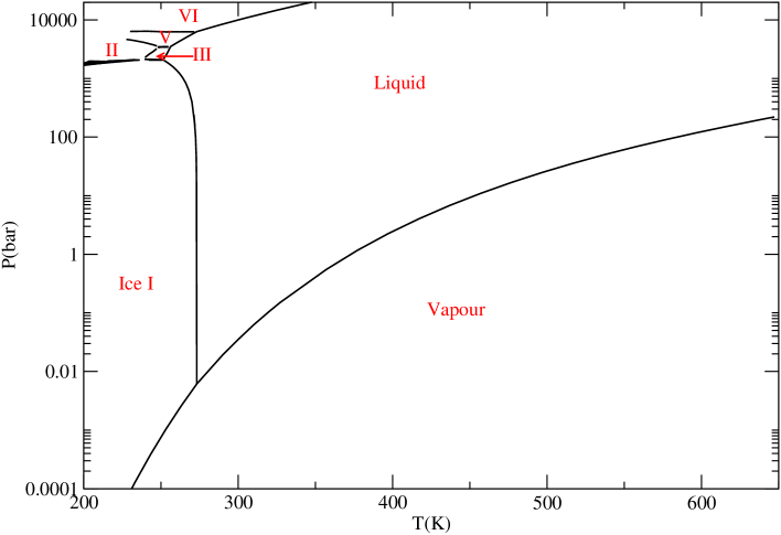
Figure 1. Experimental phase diagram of water. Roman numerals designate different ice phases. Data taken from Refs.[14, 15, 16].

Interestingly, it has become clear that such anomalous behaviour can also be reproduced by model systems interacting via spherically symmetric potentials[17]. In particular, the Hemmer-Stell potential[18], devised with the aim of describing simple systems that can exhibit multiple transitions, was shown by Jagla[19] to share with water a good number of anomalies. In this regard, Yan et. al[17], where the first to describe in this model a cascade of anomalies which is qualitatively similar to that of water (see Figure 2). Together with the Hemmer-Stell’s (or ramp) potential, a variety of interaction models have shown to be able to display peculiar behaviour, such as the Lennard-Jones+Gaussian (LJG) [20], or the square-well/square shoulder (SWSS)[2] among others. It has been argued that only the continuous version of the SWSS potential [21] yields a density anomaly, whereas other features, such as the presence of a liquid-liquid equilibrium are reproduced by the SWSS potential. These models are all characterized by the presence of two repulsive ranges of interaction. There is however an additional simple potential model that shares a good number of anomalies with these systems, namely the Gaussian core model[22]. Since this potential, being finite at zero separation, allows for complete overlap of a pair of interacting particles, it is a class of its own. One may think that together with a first repulsive range defined by the width of the Gaussian, a second range of interaction would correspond to full overlap (or the maximum of the repulsive potential), thereby casting this model into the class of two repulsive range models.

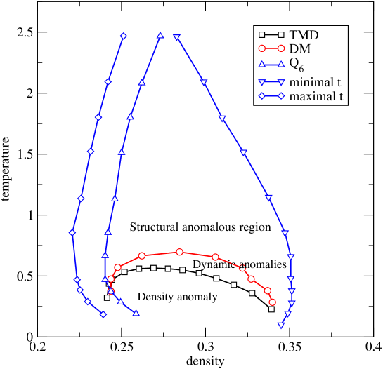
Figure 2. Cascade of anomalies for a two-short range repulsive potential (Hemmer-Stell) as studied by Yan et al.[17]. $Q_{6}$ defines the orientational order parameter, $t$ the translational order parameter (see [23]). DM designates the curve of diffusivity maxima and TMD the line of temperatures of density maxima.

Additionally, some lattice gas models have also been investigated to search for thermodynamic and structural anomalies characterized by of both isotropic[24, 25] and orientational dependent interactions[26, 27]. In this contribution we will review the simplest models that can reproduce a water-like phase behaviour and at least some of the above mentioned anomalies. Thus we will focus on one-dimensional lattice models. In this regard, the simplest system that can give a fluid-solid transition (order-disorder) in one dimension is the antiferromagnetic Ising model with two sublattices, in which the antiferromagnetic state (ordered) is mapped into a solid in lattice gas language. The model, studied in detail by Høye [28] yields a second order transition near the critical point. We will review the features of this model in the next section. Then in Section III we will see how it can be modified so as to reproduce a first order fluid-solid transition with a solid phase less dense than its fluid counterpart, following previous work by the authors[29]. In Section IV we will see how the addition of a second repulsive range brings the phase diagram closer to that of a particular class of anomalous systems such as phosphorous[30]. The two-parameter model can be thereafter tuned to yield a water-like phase diagram[31]. A purely repulsive version of the model will also be shown to reproduce the presence of density maximum, bringing much closer the analogy to water behaviour. The careful study of these and related simple yet rich physical models has been a distinctive characteristic of Prof. Johan Høye’s scientific career, representing in many cases relevant landmarks in Statistical Physics.

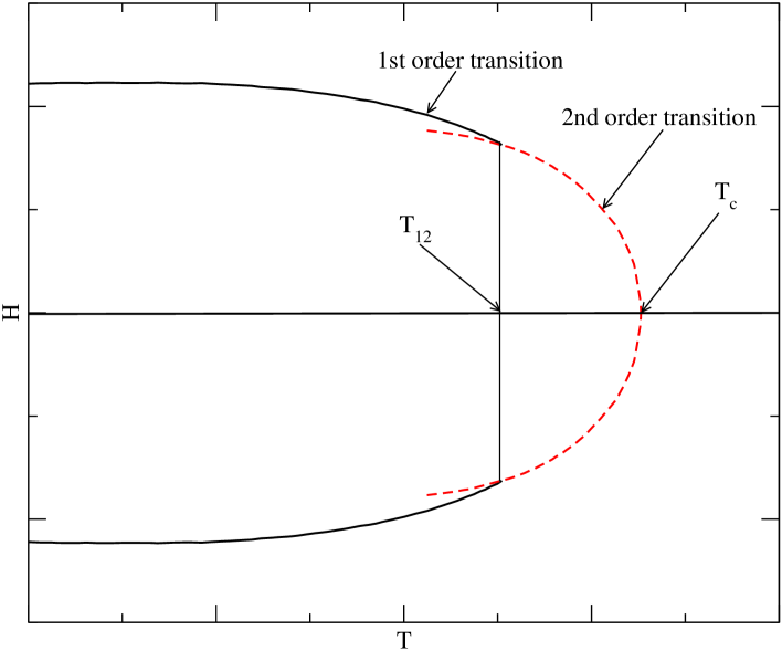
Figure 3. Qualitative phase behaviour of the one-dimensional Ising model with nearest-neighbour repulsion and an infinitely long ranged staggered mean-field acting on even numbered neighbours[28].

2. First step: antiferromagnetic models with two and three sublattices.

Back in the early seventies Høye [28] studied closely the order-disorder phase transitions of an antiferromagnetic Ising model with two sublattices, in which the antiferromagnetic state (ordered) can be mapped into a solid phase. The model is endowed with competing short range and very long range interactions, being the latter of Kac type, and acting only on even numbered spins, i.e.

$$\varphi(i-j)=\left\{\begin{array}[]{cl}-a\gamma\exp[-\gamma|i-j|],&\quad\mbox{if}\quad i-j\;\mbox{is even}\\ 0,&\quad\mbox{if}\quad i-j\;\mbox{is odd}\end{array}\right.$$ (2.1)

where $a$ is the integrated long-range interaction, i.e.

$$a=\frac{1}{2}\sum_{n=-\infty}^{\infty}\varphi(i),$$ (2.2)

and $\gamma\rightarrow 0$ being and inverse range parameter. So this long range interaction does not necessarily encourage ferromagnetic ordering. The full Hamiltonian can be written as

$$\mathcal{H}=J\sum_{i=1}^{N}s_{i}s_{i+1}+\sum_{i<j}^{N}\varphi(i-j)s_{i}s_{j}-H_{0}\sum_{i}^{N}s_{i}.$$ (2.3)

with $J>0$ being the antiferromagnetic nearest neighbour (NN) coupling constant, $N$ is the number of spins or lattice sites, $s_{i}=\pm 1$ are the spin variables, $H_{0}$ is the external field, and we consider periodic boundary conditions, i.e. $s_{i}=s_{N+i}$. This can be shown to be one of the simplest models that can yield a fluid-solid transition. However, in Ref. [28] , Høye, showed that such a system leads to a second order transition in a region close to the critical point, which for temperatures below a certain transition temperature, $T_{12}$ turns into the desired first order fluid-solid transition (see Figure 3).

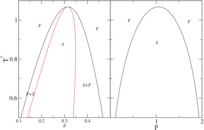
Figure 4. Phase diagram of a lattice gas with infinite NN repulsion and and three sublattices with a staggered mean field.

In order to cure this deficiency, Høye and Lomba [29], extended the model incorporating three sublattices, i.e. we considered an infinitely long ranged antiferromagnetic interaction that acts on each third spin, i.e.

$$\varphi(i-j)=\left\{\begin{array}[]{cl}3a\gamma\exp[-\gamma|i-j|],&\quad\mbox{if}\quad i-j=3n+1,\;3n+2\\ 0,&\quad\mbox{if}\quad i-j=3n\end{array}\right.$$ (2.4)

where $n$ is integer, and again the limit $\gamma\rightarrow 0$ is considered with $a>0$. The model thus constructed would have however an unwanted solid-solid transition in the middle of the order-disorder transition, due to the symmetry of the Ising model when the critical point is located at zero magnetic field or zero magnetization. The presence of a nearest neighbour hard core interaction will break the symmetry with respect to the zero field, and so remove this unwanted transition. This model can be solved using a mean field treatment to handle the long range staggered interaction and the transfer matrix method to deal with the NN antiferromagnetic coupling[32, 28]. As shown in [29] one can now get a system that yields a fluid-solid transition, in which the solid phase melts again upon compression (see Figure 4). In order to simplify the solution, the antiferromagnetic NN coupling was considered in the limit $J\rightarrow\infty$, by which then the external field $H_{0}$ must be adjusted so that $H_{0}+2J$ remains finite and spins can be turned up and down by thermal fluctuations. The model is equivalent to a lattice gas in which the particles occupy two sites. The phase diagram of Figure 4 indicates that we are now in a situation closer to a water-like behaviour: we have a model in which the solid phase melts upon compression and with a $p-T$ coexistence curve with negative slope within certain range of temperatures, i.e., pressure decreases when temperature raises. This represents a clearly “anomalous” behaviour.

3. One step beyond: two sublattices and next-to-nearest neighbour interaction

How can one improve the previous model ? On one hand we have to account for the vapour-liquid transition. This in principle can be achieved separating the mean field contribution to the free energy into a staggered term (that favours antiferromagnetic long range ordering) and an attractive term. This has to be complemented by the incorporation of a next-to-nearest neighbour interaction (NNN), which will enable to tune the location of fluid-solid equilibrium with respect to the gas-liquid critical point.

The system so constructed was studied by the author in collaboration with Høye in [30], and solved using the procedure indicated above and which will be roughly described below. The model’s Hamiltonian can be written as

$$\mathcal{H}=J\sum_{i=1}^{N}s_{i}s_{i+1}+K\sum_{i=1}^{N}s_{i}s_{i+2}+\sum_{i<j}^{N}\varphi(i-j)s_{i}s_{j}-H_{0}\sum_{i}^{N}s_{i}.$$ (3.1)

Again the $J>0$ is NN coupling, and as in [29] we let $J\rightarrow\infty$ with $H_{0}$ adjusted so that $H_{0}+2J$ remains finite, and periodic boundary conditions are imposed, but we have now a NNN interaction with a coupling constant $K>0$.

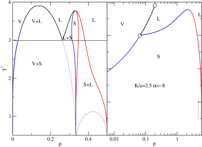
Figure 5. T-$\rho$ (left) and p-T (right) phase diagrams of a one-dimensional lattice model with NNN interactions and a staggered field. Dotted curves indicate metastable equilibria.

The lattice can be split into groups of cells made up of three sublattices in accordance with the staggered interaction (2.4). The effective fields, $H_{i}$ (acting on spins of sublattice $i$) can be expressed in terms of the mean field interaction (2.4) and the external magnetic field as

$$H_{1} = H_{0}-a(m_{2}+m_{3})$$

$$H_{2} = H_{0}-a(m_{1}+m_{3})$$

$$H_{3} = H_{0}-a(m_{1}+m_{2}),$$ (3.2)

where $m_{i}$ is the magnetization per particle of sublattice $i$. Now, we define $m_{1}=m+2u$ and $m_{2}=m_{3}=m-u$, where $m$ and $u$ are the effective and staggered magnetizations respectively. Thus the following effective field, $H_{e}$, and effective staggered field $H_{s_{e}}$, can also be defined by

$$H_{e} = \frac{1}{3}(H_{1}+H_{2}+H_{3})=H_{0}-2am$$

$$H_{s_{e}} = \frac{1}{3}(2H_{1}-H_{2}-H_{3});\;u=\frac{1}{6}(2m_{1}-m_{2}-m_{3}).$$ (3.3)

These satisfy

$$H_{0} = H_{e}+2am$$ (3.4)

$$H_{s_{e}} = 2au$$ (3.5)

The equivalency to the lattice gas gives a number density $\rho=(m+1)/2$. The reduced temperature will be defined in terms of the mean field coupling as $T^{*}=1/(\beta a)$, with $\beta=1/k_{B}T$, $k_{B}$ the Boltzmann constant, and T the absolute temperature as usual. The corresponding reduced field and NNN coupling constant will be $h^{*}=H_{0}/a$ and $K^{*}=K/a$.

Now, in order to account for the vapour-liquid transition the effect of the uniform mean field term $2am$ can be tuned, while retaining the staggered mean field contribution, $2au$. One thus ends up with

$$H_{e}=H_{0}-2\alpha am$$ (3.6)

where $\alpha$ will be a coupling term that can switch from uniform mean field attraction ($\alpha<0$) to repulsion ($\alpha>0$). Thus $\alpha\neq 1$ represents the additional uniform mean field interaction mentioned below Eq. (2.4).

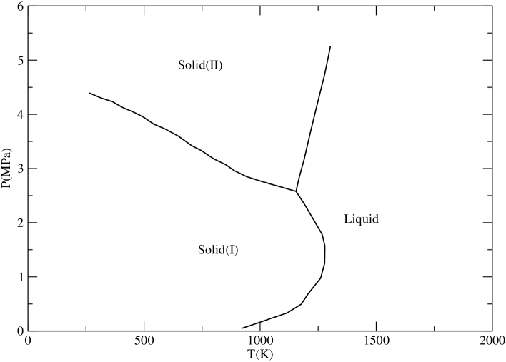
Figure 6. Phase diagram of phosphorous. Data taken from Ref.[9].

The partition function, $\lambda$, is given by the eigenvalue equation of the transfer matrix (Eqs. (23)-(25) in Ref. [30]), namely

$$\varLambda^{3}+a_{2}\varLambda^{2}+a_{1}\varLambda+a_{0}=0$$ (3.7)

where $\varLambda=\lambda^{3}$, and

$$a_{2} = -[D^{3}p^{-3}+D(2e^{-v}+e^{2v})p]$$

$$a_{1} = -[D^{2}(e^{-2v}+2e^{v})(p^{-2}-p^{2})+p^{-6}]$$

$$a_{0} = D^{3}p^{-3}(p^{-2}-p^{2})^{3},$$ (3.8)

with

$$D = \exp(-\beta H_{e})$$

$$v = \beta H_{s_{e}}\;;\;p=\exp(\beta K).$$ (3.9)

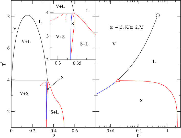
Figure 7. T-$\rho$ (left) and p-T (right) phase diagrams of a one-dimensional lattice model with NNN interactions and a staggered field with a choice of mean field attraction ($\alpha$) and NNN repulsion($K/a$) to mimic the phase diagram of water.

The magnetization $m$ and staggered magnetization $u$ result from the differentiation of the eigenvalue equation by the method used in Ref.[32], provided $\lambda$ has been calculated solving Eq. (3.7). Thus, one gets

$$m = -\frac{1}{3}\sum_{n=0}^{3}a_{n}^{\prime}\varLambda^{n}/N$$ (3.10)

$$u = -\frac{1}{3}\sum_{n=1}^{3}a_{s_{n}}^{\prime}\varLambda^{n}/N,\hskip 14.22636ptN=\sum_{n=1}^{3}na_{n}\varLambda^{n},$$ (3.11)

with

$$a_{n}^{\prime} = \frac{\partial a_{n}}{\partial(\beta H_{e})}$$

$$a_{s_{n}}^{\prime} = \frac{\partial a_{n}}{\partial(\beta H_{s_{e}})},.$$ (3.12)

Explicit expressions can be found in Ref. [30].

With this, the free energy $G$ per spin [29, 30] is given by

$$-\beta G=\ln\lambda+\beta\alpha am^{2}-\beta au^{2}.$$ (3.13)

and the corresponding lattice gas pressure $p$ reads

$$\beta p=-\beta G+\beta H+\beta K+\beta\alpha a.$$ (3.14)

We have thus all the ingredients to study the phase behaviour of our model. To that aim, we know that the phase equilibrium conditions determine that the field, $h^{*}$, and the spin free energy, $\beta G$, stay the same in both phases at equilibrium. Thus one has to solve,

$$\beta G(u=0,m_{d};T^{*}) = \beta G(u_{o},m_{o};T^{*})$$ (3.15)

$$h^{*}(u=0,m_{d};T^{*}) = h^{*}(u_{o},m_{o};T^{*})$$ (3.16)

where the subscripts _d and _o denote the disordered and ordered phases respectively. Additionally, $m_{d}$ and $h^{*}$, and $m_{o}$, $u_{o}$ and $h^{*}$ are connected via Eqs.(3.10) and (3.11). Details concerning the explicit numerical solution of these equations can be found in Refs. [29] and [30].

After a careful search over the parameter space of $K/a$ and $\alpha$, one finds that the equations (3.16) yield the phase diagram for $K/a=2.5$ and $\alpha=-8$ as shown in Figure 5. Here both the $T-\rho$ and $T-p$ phase diagrams are shown ($p$ is evaluated from Eq. (3.14)). Clearly this phase diagram departs from that of water (Figure 1) in the fact that the solid-liquid equilibrium curve starts out from the triple point with a positive instead of a negative slope. At higher densities the L-S curve reaches a liquidus point and then a region of anomalous behaviour (i.e. negative slope in the $T-p$ curve) appears. As a whole, this diagram bears some resemblance to that of phosphorous[9] depicted in Figure 6. Also in Figure 5 one observes the presence of a metastable liquid-liquid equilibrium, a feature that has been argued to be found in undercooled water (though much debated)[1, 6]. On the other hand, in the case of phosphorous, a first order liquid-liquid transition has been characterized by means of diffraction experiments in the region of high pressures and temperatures[33, 10].

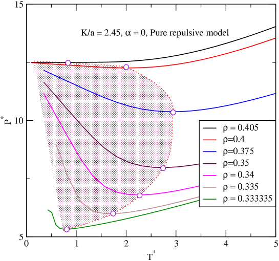
Figure 8. Temperature of maximum density curve of a one-dimensional lattice model with NNN interactions and a staggered field with purely repulsive interactions. The region of anomalous behaviour is indicated by a shaded area.

4. A water-like model

Now, the question is whether the model parameters can be tuned so as to reproduce the behaviour of water. To that aim, it seems clear from Figure 5 that the liquidus point has to be shifted into the vapour-liquid equilibrium curve. The LV curve has to be made somewhat larger in that respect so that the VL critical temperature is well above the liquidus temperature. We found that a choice of $\alpha=-15$ (a substantial increase in the dispersive interactions) and $K/a=2.75$ (a slight increase in the NNN repulsion), leads to a phase diagram in qualitative agreement with that of water, as can be seen when comparing Figures 1 and 7. One can observe in Figure 7 that now the LS equilibrium curve starts at the triple point with negative slope, as expected for a water like model. The change in density at the triple point is, on the other hand, close to one per cent, far away from the experimental $\Delta\rho/\rho\approx 10\%$ in real water. If one is to bring this to a better quantitative agreement with “real” water, both $\alpha$ and very specially $K/a$ must be fine tuned. This repulsive parameter is a key quantity since being a NNN repulsion plays an essential role in the determination of the low density solid phases. Work on this and other refinements is currently in progress.

We have seen then that a tuning of our two parameter model switches from phosphorous-like to water-like behaviour. In order to understand the key differences between both systems, one must analyze the nature of bonding in the different phases of water and phosphorous. In the case of water, both the solid and the liquid phases are dominated by the presence of relatively strong hydrogen bonds. On the other hand, low density liquid phosphorous is a molecular liquid of P₄ tetrahedra which interact via weak van der Waals forces, and the solid is formed by a layered low density orthorhombic phase[9], which upon isothermal compression melts back into a high density liquid with entangled chains and clusters of covalently bonded P atoms[34]. It is evident that attractive forces are much more important in liquid water that in the molecular P₄ liquid. This explains why in order to go from a P-like to H₂O-like phase diagram one has to substantially increase the strength of the attractive interaction (which rule the vapour-liquid equilibrium) from $\alpha=-8$ to $\alpha=-15$. As mentioned, changes in $K/a$ should make possible the fine tuning of the density change at the triple point.

Now, a question that remains to be analyzed is whether this simple model is able to reproduce the existence of density maxima for certain temperatures (at constant pressure), which is a characteristic feature of water and related systems. Using Eq. (3.14) to evaluate $p$ along isochorous curves, from elementary thermodynamics we know that those points that fulfill

$$\left(\frac{\partial p}{\partial T^{*}}\right)_{\rho}=0\;\mbox{also fulfill}\;\left(\frac{\partial\rho}{\partial T^{*}}\right)_{p}=0,$$

i.e., these state points correspond to density maxima along isobars. If one performs such a calculation with the parameters found for our water-like model, the resulting TMD curve lies in the metastable/unstable region. We have thus analyzed whether a corresponding purely repulsive model lacking a LV equilibrium can capture this feature by performing the calculations with $\alpha=0$. The result of these calculations is plotted in Figure 8. As we see the curves present clear minima which display a TMD curve that is a boundary of a thermodynamically anomalous region, in which the fluid expands upon cooling. This is actually the feature that was being sought. It remains to be seen whether a sensible choice of parameters can make compatible the existence of a TMD curve in a thermodynamically stable region with a water-like phase diagram, thus bringing our simple model to a much closer agreement with the experimental behaviour.

In summary, we have seen how one can construct a family of one dimensional lattice models that can be tuned to reproduce the behaviour of fairly complex materials such a phosphorous or water. This simple models illustrate key physical phenomena enabling a more clear understanding of the underlying physics of the anomalies found in the thermodynamics of not so simple materials. They also help expanding our knowledge of how their anomalous behaviour is originated which will in turn help in the development of more complex models that can reproduce more closely the experimental behaviour.

References

- [1] P. H. Poole, F. Sciortino, U. Essmann, and H. E. Stanley, “Phase behaviour of metastable water,,” Nature, vol. 360, pp. 324 – 328, 1992.
- [2] G. Franzese, G. Malescio, A. Skibinsky, S. V. Buldyrev, and H. E. Stanley, “Generic mechanism for generating a liquid–liquid phase transition,” Nature (London), vol. 409, pp. 692 – 695, 2001.
- [3] M. Yamada, S. Mossa, H. E. Stanley, and F. Sciortino, “Interplay between time-temperature transformation and the liquid-liquid phase transition in water,” Phys. Rev. Lett., vol. 88, p. 195701, 2002.
- [4] S. Sastry, P. G. Debenedetti, F. Sciortino, and H. E. Stanley, “Singularity-free interpretation of the thermodynamics of supercooled water,” Phys. Rev. E, vol. 53, pp. 6144 – 6154, 1996.
- [5] Z. Yan, S. V. Buldyrev, P. Kumar, N. Giovambattista, P. G. Debenedetti, and H. E. Stanley, “Structure of the first- and second-neighbor shells of simulated water: Quantitative relation to translational and orientational order,” Phys. Rev. E, vol. 76, p. 051201, 2007.
- [6] G. Franzese and H. E. Stanley, “The Widom line of supercooled water,” J. Phys.: Condens. Matter, vol. 19, p. 205126, 2007.
- [7] P. Kumar, S. Han, and H. E. Stanley, “Anomalies of water and hydrogen bond dynamics in hydrophobic nanoconfinement,” J. Phys.: Condens. Matter, vol. 21, p. 504108, 2009.
- [8] J. R. Errington and P. G. Debenedetti, “Relationship between structural order and the anomalies of liquid water,” Nature (London), vol. 409, pp. 318–322, 2001.
- [9] D. A. Young, Phase diagram of the elements. Berkeley: University of California, 1991.
- [10] G. Monaco, S. Falconi, W. A. Crichton, and M. Mezouar, “Nature of the first-order phase transition in fluid phosphorus at high temperature and pressure,” Phys. Rev. Lett., vol. 90, p. 255701, 2003.
- [11] O. Mishima, “Reversible first-order transition between two H2O amorphs at 0.2 gpa and 135 k,,” J. Chem. Phys., vol. 100, pp. 5910–5912, 1993.
- [12] I. Saika-Voivod, F. Sciortino, , and P. H. Poole, “Computer simulations of liquid silica: Equation of state and liquid-liquid phase transition,” Phys. Rev. E, vol. 63, p. 011202, 2000.
- [13] K. H. Smith, E. Shero, A. Chizmeshya, and G. H. Wolf, “The equation of state of polyamorphic germania glass: A two-domain description of the viscoelastic response,,” J. Chem. Phys., vol. 102, pp. 6851–6857, 1995.
- [14] P. Linstrom and W. Mallard, eds., NIST Chemistry WebBook, NIST Standard Reference Database Number 69. National Institute of Standards and Technology, 2011.
- [15] A. Wexler, “Vapor pressure formulation for ice,” J. Res. Nat. Bur. Stand., vol. 81A, pp. 5 – 20, 1977.
- [16] O. Mishima and S. Endo, “Phase relations of ice under pressure,” J. Chem. Phys., vol. 73, p. 2454, 1980.
- [17] Z. Yan, S. V. Buldyrev, N. Giovambattista, and H. E. Stanley, “Structural order for one-scale and two-scale potentials,” Phys. Rev. Lett., vol. 95, p. 130604, 2005.
- [18] P. C. Hemmer and G. Stell, “Fluids with several phase transitions,,” Phys. Rev. Lett., vol. 24, pp. 1284 – 1287, 1970.
- [19] E. A. Jagla, “Core-softened potentials and the anomalous properties of water,,” J. Chem. Phys., vol. 111, pp. 8980–8986, 1999.
- [20] L. B. Krott and M. C. Barbosa, “Anomalies in a waterlike model confined between plates,” J. Chem. Phys., vol. 138, p. 084505, 2013.
- [21] E. Salcedo, J. Ney M. Barraz, and M. C. Barbosa, “Relation between occupation in the first coordination shells and widom line in core-softened potentials,” J. Chem. Phys., vol. 138, p. 164502, 2013.
- [22] P. Mausbach and H.-O. May, “Static and dynamic anomalies in the gaussian core model liquid,” Fluid Phase Equilibria, vol. 249, p. 17 – 23, 2006.
- [23] T. M. Truskett, S. Torquato, and P. G. Debenedetti, “Towards a quantification of disorder in materials: Distinguishing equilibrium and glassy sphere packings,” Phys. Rev. E, vol. 62, p. 993 – 1001, 2000.
- [24] A. L. Balladares and M. C. Barbosa, “Density anomaly in core-softened lattice gas,” J. Phys.: Condens. Matter, vol. 16, pp. 8811–8822, 2004.
- [25] A. B. de Oliveira and M. C. Barbosa, “Density anomaly in a competing interactions lattice gas model,” J. Phys.: Condens. Matter, vol. 17, pp. 399–411, 2005.
- [26] M. Girardi, A. L. Balladares, V. B. Henriques, and M. C. Barbosa, “Liquid polymorphism and density anomaly in a three-dimensional associating lattice gas,” J. Chem. Phys., vol. 126, p. 064503, 2007.
- [27] M. A. A. Barbosa and V. B. Henriques, “Frustration and anomalous behavior in the Bell-Lavis model of liquid water,” Phys. Rev. E, vol. 77, p. 051204, 2008.
- [28] J. S. Høye, “Spin model with antiferromagnetic and ferromagnetic interactions,,” Phys. Rev. B, vol. 6, pp. 4261 – 4266, 1972.
- [29] J. S. Høye and E. Lomba, “Phase behavior of a simple lattice model with a two-scale repulsive interaction,,” J. Chem. Phys., vol. 129, p. 024501, 2008.
- [30] J. S. Høye, E. Lomba, and N. G. Almarza, “One- and three-dimensional lattice models with two repulsive ranges: simple systems with complex phase behaviour,” Mol. Phys., vol. 107, pp. 321 – 330, 2009.
- [31] J. S. Høye and E. Lomba, “A simple one-dimensional lattice model with water-like phase behaviour,” Mol. Phys., vol. 108, pp. 51 – 55, 2010.
- [32] W. K. Theumann and J. S. Høye, “Ising chain with several phase transitions,” J. Chem. Phys., vol. 55, p. 4159, 1971.
- [33] Y. Katayama, T. Mizutani, W. Utsumi, O. Shimomura, M. Yamakata, and K. Funakoshi, “A first-order liquid-liquid phase transition in phosphorus,,” Nature (London), vol. 403, pp. 170–174, 2000.
- [34] T. Morishita, “Polymeric liquid of phosphorus at high pressure: first-principles molecular-dynamics simulations,” Phys. Rev. B, vol. 66, p. 054204, 2002.