Majorization approach to entropic uncertainty relations for coarse-grained observables

Abstract

We improve the entropic uncertainty relations for position and momentum coarse-grained measurements. We derive the continuous, coarse-grained counterparts of the discrete uncertainty relations based on the concept of majorization. The obtained entropic inequalities involve two Rényi entropies of the same order, and thus go beyond the standard scenario with conjugated parameters. In a special case describing the sum of two Shannon entropies the majorization-based bounds significantly outperform the currently known results in the regime of larger coarse graining, and might thus be useful for entanglement detection in continuous variables.

I Introduction

The optimal entropic uncertainty relation for a couple of conjugate continuous variables (position and momentum) is known for almost 40 years BBM . One decade later, entropic formulation of the uncertainty principle has as well been developed in the discrete settings Deutsch ; MU . Even though, the topic of entropic uncertainty relations (EURs) has a long history (for a detailed review see Wehner ; IBBLR ), one can observe a recent increase of interest within the quantum information community leading to several improvements deVicente ; deVicenteComm ; Partovi ; my ; oni ; Coles ; RPZ ; Korzekwa1 ; Bosyk1 ; Bosyk2 ; Bosyk3 ; Kaniewski or even a deep asymptotic analysis of different bounds Banach . This is quite understandable, because the entropic uncertainty relations have various applications, for example in entanglement detection Lewenstein ; Partovi2 ; Rastegin1 ; ConEnt1 ; ConEnt2 , security of quantum protocols crypto ; crypto2 , quantum memory Berta ; memory2 or as an ingredient of Einstein–Podolsky–Rosen steering criteria Steering1 ; EPR . Moreover, the recent discussion HeisWerner about the original Heisenberg idea of uncertainty, led to the entropic counterparts of the noise-disturbance uncertainty relation HeisEntropic ; Rastegin2 (also obtained with quantum memory ColFur ).

My favorite example of entropic description of uncertainty partoviOld ; IBB1 ; IBB2 is situated in between the continuous and the discrete scenario. Continuous position and momentum variables, while studied with the help of coarse-grained measurements lead to discrete probability distributions. This particular formulation of the uncertainty principle has been long ago recognized Lenard ; Lahti ; Lahti2 to faithfully capture the spirit of position-momentum duality. It also carries a deep physical insight, since the coarse-grained version of the Heisenberg uncertainty relation is non-trivial for any coarse-graining (given in terms of two widths $\Delta$ and $\delta$ in positions and momenta respectively) provided that the both widths are finite OptCon . On the practical level, coarse-grained entropic relations are experimentally useful for entanglement ConEnt2 ; Megan and steering detection Steering1 in continuous variable schemes. The aim of this paper is thus to strengthen the theoretical and experimental tools based on the coarse-grained EURs by taking an advantage of the recent improvements of discrete entropic inequalities, in particular, the one based on majorization RPZ .

Let me start with a brief description of the entropic uncertainty landscape, with a special emphasis on the majorization approach developed recently. The standard position-momentum scenario deals with the sum of the continuous Shannon (or in general Rényi) entropies $-\int dz\rho\left(z\right)\ln\rho\left(z\right)$ calculated for both densities $\rho\left(x\right)=|\psi\left(x\right)|^{2}$ and $\tilde{\rho}\left(p\right)=|\tilde{\psi}\left(p\right)|^{2}$ describing positions and momenta respectively. The position and momentum wave functions are mutually related by the Fourier transformation. The discrete EURs rely on the notion of the Rényi entropy of order $\alpha$

$$H_{\alpha}\left[P\right]=\frac{1}{1-\alpha}\ln\sum_{i}P_{i}^{\alpha},$$ (1)

and the sum-inequalities of the general form

$$H_{\alpha}\left[P\left(A;\varrho\right)\right]+H_{\beta}\left[P\left(B;\varrho\right)\right]\geq B_{\alpha\beta}\left(A,B\right)$$ (2)

valid for any density matrix $\varrho$, and two non-degenerate observables $A$ and $B$. If by $\bigl{|}a_{i}\bigr{\rangle}$ and $\bigl{|}b_{j}\bigr{\rangle}$ we denote the eigenstates of the two observables in question, the associated probability distributions entering (2) are:

$$P_{i}\left(A;\varrho\right)=\bigl{\langle}a_{i}\bigr{|}\varrho\bigl{|}a_{i}\bigr{\rangle}\;\;\textrm{and }\;P_{j}\left(B;\varrho\right)=\bigl{\langle}b_{j}\bigr{|}\varrho\bigl{|}b_{j}\bigr{\rangle}.$$ (3)

The lower bound $B_{\alpha\beta}$ does not depend on $\varrho$, but only on the unitary matrix $U_{ij}=\bigl{\langle}a_{i}\bigr{|}b_{j}\bigr{\rangle}$. For instance, the most recognized result by Maassen and Uffink MU gives the bound $-2\ln\max_{i,j}|U_{ij}|$, valid whenever

$$\frac{1}{\alpha}+\frac{1}{\beta}=2.$$ (4)

The couple $(\alpha,\beta)$ constrained as in Eq. (4) is often referred to as the conjugate parameters.

I.1 Majorization entropic uncertainty relations

In the majorization approach one looks for the probability vectors $Q\left(A,B\right)$ and $W\left(A,B\right)$ which majorize the tensor product my ; oni and the direct sum RPZ of the involved distributions (3):

$$P\left(A;\varrho\right)\otimes P\left(B;\varrho\right)\prec Q\left(A,B\right),$$ (5)

$$P\left(A;\varrho\right)\oplus P\left(B;\varrho\right)\prec\{1\}\oplus W\left(A,B\right).$$ (6)

The majorization relation $x\prec y$ between any two $D$-dimensional probability vectors implies that for all $n\leq D$ we have $\sum_{k=1}^{n}x_{k}^{\downarrow}\leq\sum_{k=1}^{n}y_{k}^{\downarrow}$, with a necessary equality when $n=D$. In agreement with the usual notation, the symbol $\downarrow$ denotes the decreasing order, what means that $\bigl{(}x^{\downarrow}\bigr{)}{}_{k}\geq\bigl{(}x^{\downarrow}\bigr{)}{}_{l}$, for all $k\leq l$. In the case when the vectors compared in (5) and (6) are of different size, the shorter vector shall be completed by a proper number of coordinates equal to $0$. The tensor product $x\otimes y$ (also called the Kronecker product) is a $D^{2}$-dimensional probability vector with the coefficients equal to

$$x_{1}y_{1},x_{1}y_{2},\ldots,x_{1}y_{D},\ldots,x_{D}y_{1},x_{D}y_{2},\ldots,x_{D}y_{D},$$ (7)

while the direct sum $x\oplus y$ is a $2D$-dimensional probability vector given by

$$x_{1},x_{2},\ldots,x_{D},y_{1},y_{2},\ldots,y_{D}.$$ (8)

One of the most important properties of the Rényi entropy of any order $\alpha$ is its additivity

$$H_{\alpha}\left[x\right]+H_{\alpha}\left[y\right]=H_{\alpha}\left[x\otimes y\right].$$ (9)

Moreover, in the special case of the Shannon entropies ($H_{1}\left[\cdot\right]\equiv H\left[\cdot\right]$) one easily finds that

$$H\left[x\right]+H\left[y\right]=H\left[x\oplus y\right].$$ (10)

Since the presumed majorization relations (5, 6) are valid for every $\varrho$, the Schur-concavity of the Rényi (Shannon) entropy together with (9, 10) immediately lead to the corresponding bounds $B_{\alpha\alpha}=H_{\alpha}\left[Q\right]$ my ; oni and $B_{11}=H\left[W\right]$ RPZ . Due to the subadditivity property of the function $\ln(1+z)$ the validity of the latter bound can be extended RPZ to the range $\alpha\leq 1$ (in that case the function $\sum_{i}z_{i}^{\alpha}$ is as well Schur-concave), i.e. $B_{\alpha\alpha}^{\alpha\leq 1}=H_{\alpha}\left[W\right]$. On the other hand, when $\alpha>1$, this bound can be appropriately modified to the weaker form RPZ

$$B_{\alpha\alpha}^{\alpha>1}\left[W\right]=\frac{2}{1-\alpha}\left[\ln\left(1+\sum_{i}W_{i}\right)-\ln 2\right].$$ (11)

The whole families of the vectors $Q\left(A,B\right)$ and $W\left(A,B\right)$ fulfilling (5) and (6) have been explicitly constructed in my ; oni and RPZ respectively. The aim of the present paper is to obtain the counterpart of the majorizing vector $W\left(A,B\right)$ applicable to the position-momentum coarse-grained scenario described in detail in the forthcoming Section I.2. In Section II we derive this vector using the sole idea of majorization, so that we shall omit here a detailed prescription established in RPZ . We restrict the further discussion to the direct-sum approach, since for $\alpha\leq 1$ (this case covers the sum of two Shannon entropies), the direct-sum entropic uncertainty relation is always stronger than the corresponding tensor-product EUR RPZ .

I.2 Entropic uncertainty relations for coarse-grained observables

The last set of ingredients we shall introduce, contains the coarse-grained probabilities together with their EURs. Due to coarse-graining, the continuous densities $\rho\left(x\right)$ and $\tilde{\rho}\left(p\right)$ become the discrete probabilities:

$$q_{k}^{\Delta}=\int_{k^{-}\Delta}^{k^{+}\Delta}dx\,\rho\left(x\right),\quad p_{l}^{\delta}=\int_{l^{-}\delta}^{l^{+}\delta}dp\,\tilde{\rho}\left(p\right),$$ (12)

with $k^{\pm}=k\pm 1/2$, $l^{\pm}=l\pm 1/2$ and $k,l\in\mathbb{Z}$. The sum of the Rényi entropies $H_{\alpha}\bigl{[}q^{\Delta}\bigr{]}$ and $H_{\beta}\bigl{[}p^{\delta}\bigr{]}$ calculated for the probabilities (12) is lower-bounded by OptCon

$$B_{\alpha\beta}\left(\Delta,\delta\right)=\max\left[\mathcal{B}_{\alpha}\left(\Delta\delta/\hbar\right);\mathcal{R}\left(\Delta\delta/\hbar\right)\right],$$ (13)

where IBB2

$$\mathcal{B}_{\alpha}\left(\gamma\right)=-\frac{1}{2}\left(\frac{\ln\alpha}{1-\alpha}+\frac{\ln\beta}{1-\beta}\right)-\ln\left(\gamma/\pi\right),$$ (14)

and OptCon

$$\mathcal{R}\left(\gamma\right)=-\ln\left(\gamma/2\pi\right)-\!2\ln R_{00}\left(\gamma/4,1\right)\!\geq 0.$$ (15)

Once more the above results are valid only for conjugate parameters (4), so that we label the bound (14) only by the index $\alpha$. The function $R_{00}\left(\xi,\eta\right)$ is the “00” radial prolate spheroidal wave function of the first kind abr . When $\gamma\ll 1$, the spheroidal term in (15) becomes negligible and we have

$$\mathcal{R\left(\gamma\right)}\approx\mathcal{B}_{1}\left(\gamma\right)+\ln 2-1,$$ (16)

so that the bound (14) dominates in this regime. In the opposite case, when $\gamma>e\pi\approx 8.54$ the bound (14) is negative, so starting from some smaller ($\alpha$-dependent) value of $\gamma$ the second bound $\mathcal{R\bigl{(}\gamma\bigr{)}}$ becomes significant.

II Direct-sum majorization for coarse-grained observables

After the short but comprehensive introduction, we are in position to formulate the main result of this paper. Assume that a sum of any $M$ position probabilities $q^{\Delta}$ and any $N$ momentum probabilities $p^{\delta}$ is bounded by $1+G_{MN}\left(\gamma\right)$, that is ($\gamma=\Delta\delta/\hbar$)

$$q_{k_{1}}^{\Delta}+\ldots+q_{k_{M}}^{\Delta}+p_{l_{1}}^{\delta}+\ldots+p_{l_{N}}^{\delta}\leq 1+G_{MN}\left(\gamma\right),$$ (17)

for some indices $k_{1}\neq k_{2}\neq\ldots\neq k_{M}$ and $l_{1}\neq l_{2}\neq\ldots\neq l_{N}$. We implicitly assume here that $G_{MN}\left(\gamma\right)$ does not depend on the specific choice of the probabilities in the sum (it bounds any choice), and that $G_{MN}\left(\gamma\right)\leq 1$ since the left hand side of (17) cannot exceed $2$. Denote further by

$$F_{J}\left(\gamma\right)=\max_{0\leq M\leq J}G_{M,J-M}\left(\gamma\right).$$ (18)

Assume now that $F_{J}\left(\gamma\right)$, $J=1,2,\ldots\infty$ is an increasing sequence

$$F_{J+1}\left(\gamma\right)\geq F_{J}\left(\gamma\right).$$ (19)

If that happens, the construction of the vector $W\left(\gamma\right)$ applicable to the direct-sum majorization relation, i.e. such that $q^{\Delta}\oplus p^{\delta}\prec\{1\}\oplus W\left(\gamma\right)$ can be patterned after RPZ :

$$W_{i}\left(\gamma\right)=F_{i+1}\left(\gamma\right)-F_{i}\left(\gamma\right),$$ (20)

for $i=1,2,\ldots\infty$. Due to (19) the coefficients $W_{i}\left(\gamma\right)$ are all non-negative, so that they form a probability vector. Note that $F_{1}\left(\gamma\right)\equiv 0$, since one picks up only a single probability ($M=1$, $N=0$ or $M=0$, $N=1$), and that $F_{\infty}\left(\gamma\right)\equiv 1$, because whenever the quantum state is localized (in position or momentum) in a single bin, the left hand side of (17) is equal to $2$. This is in accordance with an expectation that $W\left(\gamma\right)$ is the probability vector.

One can check by a direct inspection that

$$1+\sum_{i=1}^{J-1}W_{i}^{\downarrow}\bigl{(}\gamma\bigr{)}\geq 1+\sum_{i=1}^{J-1}W_{i}\bigl{(}\gamma\bigr{)}=1+F_{J}\left(\gamma\right),$$ (21)

what together with (17) and (18) is the essence of majorization. As in the case of discrete majorization my ; RPZ , there is a whole family (labeled by $n=2,\ldots\infty$) of majorizing vectors $W^{(n)}\left(\gamma\right)$ given by the prescription $W_{i}^{(n)}\equiv W_{i}$ for $i<n$, $W_{n}^{(n)}=1-F_{n}$, and $W_{i}^{(n)}\equiv 0$ when $i>n$. In that notation, the basic vector (20) is equivalent to $W^{(\infty)}\left(\gamma\right)$, and the following majorization chain does hold

$$W^{(2)}\!\succ W^{(3)}\!\succ\ldots\!\succ W^{(n)}\!\succ W^{(n+1)}\!\succ\ldots\!\succ W^{(\infty)}\equiv W.$$ (22)

The remaining task is to find the candidates for the coefficients $F_{J}\left(\gamma\right)$. To this end we shall define two sets:

$$X\left(\Delta\right)=\bigcup_{a=1}^{M}\left[k_{a}^{-}\Delta,k_{a}^{+}\Delta\right],\qquad Y\left(\delta\right)=\bigcup_{b=1}^{N}\left[l_{b}^{-}\Delta,l_{b}^{+}\Delta\right],$$ (23)

which are simply the unions of intervals associated with the probabilities present in (17). The measures of these sets are equal to $M\Delta$ and $N\delta$ respectively. Eq. (17) rewritten in terms of the above sets simplifies to the form

$$\int_{X\left(\Delta\right)}dx\,\rho\left(x\right)+\int_{Y\left(\delta\right)}dp\,\tilde{\rho}\left(p\right)\leq 1+G_{MN}\left(\gamma\right).$$ (24)

Following Lenard Lenard , we shall further introduce two projectors $\hat{\mathcal{Q}}$ and $\hat{\mathcal{P}}$, such that for any function $f\left(x\right)$, the function $\bigl{(}\hat{\mathcal{Q}}f\bigr{)}\left(x\right)$ has its support equal to $X\left(\Delta\right)$ and the Fourier transform of the function $\bigl{(}\hat{\mathcal{P}}f\bigr{)}\left(x\right)$ is supported in $Y\left(\delta\right)$. If both $X\left(\Delta\right)$ and $Y\left(\delta\right)$ are intervals, then according to Theorem 4 from Lahti2 (this theorem in fact formalizes the content of Eq. 17 from Lahti ) the formal candidate for $G_{MN}\left(\gamma\right)$ is the square root of the largest eigenvalue $\lambda_{0}$ of the compact, positive operator $\hat{\mathcal{Q}}\hat{\mathcal{P}}\hat{\mathcal{Q}}$. Due to Proposition 11 (including the discussion around it) from Lenard , the above statement remains valid for any sets $X\left(\Delta\right)$ and $Y\left(\delta\right)$. As concluded by Lenard, this is a generalization of the seminal results by Landau and Pollak LandauPollak , who for the first time quantified uncertainty using spheroidal functions. It however happens Price , that $\lambda_{0}$ has the largest value exactly in the interval case, so that it can always be upper bounded by the eigenvalue found by Landau and Pollak:

$$\lambda_{0}\leq\frac{\xi}{2\pi\hbar}\left[R_{00}\left(\xi/4\hbar,1\right)\right]^{2},$$ (25)

with $\xi$ being the product of the measures of the two sets in question, that is $\xi=\bigl{(}M\Delta\bigr{)}\bigl{(}N\delta\bigr{)}$. Since the right hand side of (25) is an increasing function of $\xi$, we can easily find the maximum in (18). The maximal value of $MN$ with fixed $M+N$ is given by possibly equal contributions of the both numbers. Since $M$ and $N$ are integers we finally get

$$F_{J}\left(\gamma\right)=\sqrt{\frac{\gamma\left\lceil J/2\right\rceil\left\lfloor J/2\right\rfloor}{2\pi}}R_{00}\left(\frac{\gamma\left\lceil J/2\right\rceil\left\lfloor J/2\right\rfloor}{4},1\right),$$ (26)

where $\left\lceil\cdot\right\rceil$ and $\left\lfloor\cdot\right\rfloor$ denote the integer valued ceiling and floor functions respectively . If $J$ is odd then $\left\lceil J/2\right\rceil\left\lfloor J/2\right\rfloor=\left(J^{2}-1\right)/4$, and $\left\lceil J/2\right\rceil\left\lfloor J/2\right\rfloor=J^{2}/4$ in the simpler case when $J$ is an even number. Note that the functions (26) form the increasing sequence as desired.

The major result of the above considerations is thus the family of new majorization entropic uncertainty relations ($n=2,\ldots\infty$):

$$H_{\alpha}\bigl{[}q^{\Delta}\bigr{]}+H_{\alpha}\bigl{[}p^{\delta}\bigr{]}\geq\mathcal{R}_{\alpha}^{(n)}\left(\Delta\delta/\hbar\right)\equiv H_{\alpha}\bigl{[}W^{(n)}\left(\Delta\delta/\hbar\right)\bigr{]},$$ (27)

valid for $\alpha\leq 1$. As mentioned in Section I.1 the case of the Shannon entropy directly follows from (10), while the range $\alpha<1$ is obtained due to the subadditivity of $\ln(1+z)$. In the case $\alpha>1$ we need to replace the majorization bound according to (11), and obtain $\mathcal{R}_{\alpha}^{(n)}\left(\gamma\right)\equiv B_{\alpha\alpha}^{\alpha>1}\bigl{[}W^{(n)}\left(\gamma\right)\bigr{]}$.

III Discussion

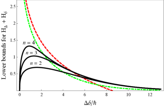
Figure 1: (Color online) As a comparison, I plot the previously known lower bounds $\mathcal{B}_{1}$ (red dashed line), and $\mathcal{R}$ (green dashed–dotted line), together with the new majorization bounds (black solid lines), labeled by $n=2,3,4$. By $H_{\Delta}$ and $H_{\delta}$ I denote $H_{1}\bigl{[}q^{\Delta}\bigr{]}$ and $H_{1}\bigl{[}p^{\delta}\bigr{]}$ respectively. From the value $\Delta\delta/\hbar\approx 4.8231$ in which the black line ($n=4$) intersects the red dashed line, the new bounds improve the previously known results.

The comparison of the previous bounds (14) and (15) with the new majorization results is presented in Fig. 1, for the case of the Shannon entropy ($\alpha=1=\beta$). I depicted the first three majorization-based bounds (black, solid lines) since they are sufficient to capture the whole content of the new uncertainty relations. First of all, only the bound for $n=2$ is slightly weaker than the remaining majorization bounds in the regime of larger $\gamma$, while there is no difference between $n=3$, $n=4$ and other (not presented) values of $n$. For $\gamma\rightarrow\infty$, all the black curves exhibit the same behavior, so that one can take an advantage of the asymptotic expansion Fuchs

$$\frac{\gamma}{2\pi}\left[R_{00}\left(\gamma/4,1\right)\right]^{2}\sim 1-2\sqrt{\pi\gamma}e^{-\gamma/2},$$ (28)

in order to show that

$$\mathcal{R}_{1}^{(n)}\left(\gamma\right)\sim\frac{\sqrt{\pi}}{2}\gamma^{3/2}e^{-\gamma/2},$$ (29)

for all $n=2,\ldots\infty$. The same expansion studied for the previous bound (15) leads to

$$\mathcal{R}\left(\gamma\right)\sim 2\sqrt{\pi\gamma}e^{-\gamma/2}.$$ (30)

The asymptotic value of (29) is larger than (30) by a divergent factor $\gamma/4$. Since the bound (15) for the sum of two Shannon entropies is always weaker than the couple $\mathcal{B}_{1}\left(\gamma\right)$ and $\mathcal{R}_{1}^{(3)}\left(\gamma\right)$, it is in this case sufficient to use only these two bounds. Obviously, the bound $\mathcal{R}\left(\gamma\right)$ remains useful (as being always non-negative) for the conjugated parameters $(\alpha,\beta)$ with $\alpha\neq\beta$, when the majorization bounds do not apply. Let me remind, that in the limiting case $\alpha=1/2$, $\beta=\infty$, the bound $\mathcal{R}\left(\gamma\right)$ is optimal and can be saturated for any value of $\gamma$.

While increasing the number $n$ we do not change the tail of the bound, we still substantially improve the area of small $\gamma$. Taking the limit $\gamma\rightarrow 0$ one can recognize that the optimal majorization bound $\mathcal{R}_{1}^{(\infty)}\left(\gamma\right)$, behaves like $-\frac{1}{2}\ln\gamma$, so is still far below the bound $\mathcal{B}_{1}\left(\gamma\right)$. To show that property one needs to associate $i\sqrt{\gamma}$ in (20) with a continuous variable $z$, so that

$$W_{i}\left(\gamma\right)\rightarrow\sqrt{\gamma}\frac{d}{dz}\left[\frac{z}{2\sqrt{2\pi}}R_{00}\left(z^{2}/16,1\right)\right],$$ (31)

and use the definition of the Riemann integral. This kind of behavior is somehow typical in the majorization approach to entropic uncertainty relations. In the discrete case, the tensor-product EUR (weaker than the direct-sum EUR used in this paper) can outperform the Maassen-Uffink result in more than $98\%$ of cases my , even for a small dimension of the Hilbert space equal to $5$. But the Maassen-Uffink lower bound MU always dominates when $U_{ij}$ is sufficiently close to the Fourier matrix, so that both eigenbases of the observables $A$ and $B$ become mutually unbiased. The continuous limit $\gamma\rightarrow 0$ is of exactly the same sort, since the resulting continuous densities originate from the wave functions in position and momentum spaces, which are related by the Fourier transformation. Note that the behavior in the limit $\gamma\rightarrow 0$ does not thus permit us to derive counterparts of the continuous EURs BBM ; IBB2 ; Vignat , valid for $\beta=\alpha$.

IV Conclusions

The direct-sum majorization entropic uncertainty relation for coarse-grained observables given by Eq. (27) is the first known bound in the case $\beta=\alpha$ and $\alpha\neq 1$. In the Shannon case, the bound (13) holds as well and the comparison of all bounds is depicted in Fig. 1. The new bounds (black, solid lines) significantly improve the previously known results in the regime of $\gamma\geq 4.8231$ (this threshold value is an intersection point between the red dashed line and the black line labeled by $n=4$). Such regime of relevance ($\gamma\geq 4.8231$) is of practical importance. In ConEnt2 , entanglement of a two-mode Gaussian state has been experimentally confirmed with the coarse-graining widths $\Delta=17\Delta_{1}$ and $\delta=15\delta_{1}$, where $\Delta_{1}=0.0250\textrm{mm}$ and $\delta_{1}/\hbar=1.546\textrm{mm}^{-1}$. To construct the entanglement criteria, one needs to put $\gamma=\Delta\delta/2\hbar$ inside the underlying uncertainty relation (the factor of $1/2$ comes from different normalization of global quadratures), so that the above numbers boil down to the value $\gamma=4.9279$. Even though, we observe a tiny overlap between the regime in which the new EUR outperforms the previous results and the parameters from ConEnt2 , for slightly larger coarse graining, say $\gamma=7$, the value of the bound increases by $60\%$ because $\mathcal{R}_{1}^{(3)}\left(7\right)/\mathcal{B}_{1}\left(7\right)=1.609$. This however suggests, that with the new bound at hand, one could improve the performance of the entanglement criteria and possibly detect entanglement beyond the cases reported in ConEnt2 . The better detection ability might become important while dealing with multipartite entanglement Saboia , since due to the increasing number of degrees of freedom, the coarse-grained measurements might appear to be the one feasible experimental method personal .

In the discrete scenario with almost mutually unbiased bases the Maassen–Uffink bound always outperforms the majorization approach. It however still can be improved with the help of the monotonicity property of the relative entropy Coles , or by combining the former approach with the majorization techniques RPZ . In the continuous case this type of analysis is far more difficult, since we actually do not have in our disposal the unitary matrix $U$ such that $a_{k}=\sum_{l}U_{kl}b_{l}$ and $a_{k},b_{l}$ are the probability amplitudes reproducing (12),

$$q_{k}^{\Delta}=|a_{k}|^{2},\qquad p_{l}^{\delta}=|b_{l}|^{2}.$$ (32)

From the beginning we deal with the per se probabilities $q_{k}^{\Delta}$ and $p_{l}^{\delta}$. This fundamental difference can be overcome if one introduces an additional degree of freedom arxivMoj ; RusLas ; OptCon corresponding to the orthonormal bases on the intervals $\left[k_{a}^{-}\Delta,k_{a}^{+}\Delta\right]$ and $\left[l_{b}^{-}\Delta,l_{b}^{+}\Delta\right]$. Even though, this approach brings the valid unitary matrix $U$, the remaining optimization required by Coles becomes a challenging task.

- (1) I. Białynicki-Birula and J. Mycielski, Commun. Math. Phys. 44, 129 (1975).
- (2) D. Deutsch, Phys. Rev. Lett. 50, 631 (1983).
- (3) H. Maassen and J. M. B. Uffink, Phys. Rev. Lett. 60, 1103 (1988).
- (4) S. Wehner and A. Winter, New J. Phys. 12, 025009 (2010).
- (5) I. Białynicki-Birula and Ł. Rudnicki Entropic uncertainty relations in quantum physics in Statistical Complexity, ed. K D Sen (Berlin: Springer) pp 1–34 (2011).
- (6) J. I. de Vicente and J. Sanchez-Ruiz, Phys. Rev. A 77, 042110 (2008).
- (7) G. M. Bosyk, M. Portesi, A. Plastino, and S. Zozor, Phys. Rev. A 84, 056101 (2011).
- (8) M. H. Partovi, Phys. Rev. A 84, 052117 (2011).
- (9) Z. Puchała, Ł. Rudnicki, and K. Życzkowski, J. Phys. A 46, 272002 (2013).
- (10) S. Friedland, V. Gheorghiu, and G. Gour, Phys. Rev. Lett. 111, 230401 (2013).
- (11) P. Coles and M. Piani, Phys. Rev. A 89, 022112 (2014).
- (12) Ł. Rudnicki, Z. Puchała, and K. Życzkowski, Phys. Rev. A 89, 052115 (2014).
- (13) K. Korzekwa, M. Lostaglio, D. Jennings, and T. Rudolph, Phys. Rev. A 89, 042122 (2014).
- (14) S. Zozor, G. M. Bosyk, and M. Portesi, J. Phys. A 46, 465301 (2013).
- (15) G. M. Bosyk, S. Zozor, M. Portesi, T. M. Osán, and P. W. Lamberti, Phys. Rev. A 90, 052114 (2014).
- (16) S. Zozor, G. M. Bosyk, and M. Portesi, J. Phys. A 47, 495302 (2014).
- (17) J. Kaniewski, M. Tomamichel, and S. Wehner, Phys. Rev. A 90, 012332 (2014).
- (18) R. Adamczak, R. Latała, Z. Puchała, and K. Życzkowski, arXiv:1412.7065 (2015).
- (19) O. Gühne and M. Lewenstein, Phys. Rev. A 70, 022316 (2004).
- (20) M. H. Partovi, Phys. Rev. A 86, 022309 (2012).
- (21) A. E. Rastegin, arXiv:1407.7333 (2014).
- (22) S. P. Walborn, B. G. Taketani, A. Salles, F. Toscano, and R. L. de Matos Filho, Phys. Rev. Lett. 103, 160505 (2009).
- (23) D. S. Tasca, Ł. Rudnicki, R.M. Gomes, F. Toscano, and S. P. Walborn, Phys. Rev. Lett. 110, 210502 (2013).
- (24) I. B. Damgaard, S. Fehr, R. Renner, L. Salvail, and C. Schaffner, in Advances in Cryptography—CRYPTO, LNCS (Springer, New York, 2007), Vol. 4622, pp. 360–378.
- (25) N. H. Y. Ng, M. Berta, and S. Wehner, Phys. Rev. A 86, 042315 (2012).
- (26) M. Berta, M. Christandl, R. Colbeck, J. M. Renes, and R. Renner, Nat. Phys. 6, 659 (2010).
- (27) T. Pramanik, P. Chowdhury, and A. S. Majumdar, Phys. Rev. Lett. 110, 020402 (2013).
- (28) J. Schneeloch, P. B. Dixon, G. A. Howland, C. J. Broadbent, and J. C. Howell, Phys. Rev. Lett. 110, 130407 (2013).
- (29) J. Schneeloch, C. J. Broadbent, and J. C. Howell, Phys. Lett. A 378, 766 (2014).
- (30) P. Busch, P. Lahti, and R. F. Werner, Phys. Rev. Lett. 111, 160405 (2013).
- (31) F. Buscemi, M. J. W. Hall, M. Ozawa, and M. M. Wilde, Phys. Rev. Lett. 112, 050401 (2014).
- (32) A. E. Rastegin, arXiv:1406.0054 (2014).
- (33) P. J. Coles, F. Furrer, Phys. Lett. A 379, 105–112 (2015).
- (34) M. H. Partovi, Phys. Rev. Lett. 50, 1883 (1983).
- (35) I. Bialynicki-Birula, Phys. Lett. A 103, 253 (1984).
- (36) I. Bialynicki-Birula, Phys. Rev. A 74, 052101 (2006).
- (37) A. Lenard, J. Functional Analysis 10, 410 (1972).
- (38) P. Lahti, Rep. Math. Phys. 23, 289 (1986).
- (39) P. Busch, T. Heinonen, P. Lahti, Physics Reports 452, 155 (2007).
- (40) Ł. Rudnicki, S. P. Walborn, and F. Toscano, Phys. Rev. A 85, 042115 (2012).
- (41) M. R. Ray and S. J. van Enk, Phys. Rev. A 88, 042326 (2013).
- (42) M. Abramowitz and I. A. Stegun, Handbook of Mathematical Functions. Dover, New York, (1964).
- (43) H. J. Landau and H. O. Pollak, Bell System Tech. J. 40, 65 (1961).
- (44) M. Cowling and J. Price, SIAM J. Math. Anal. 15, 151 (1984).
- (45) W. H. J. Fuchs, J. Math. Anal. Appl. 9, 317 (1964).
- (46) S. Zozor and C. Vignat, Physica A 375 499 (2007).
- (47) A. Saboia, A. T. Avelar, S. P. Walborn, and F. Toscano, arXiv:1407.7248 (2014).
- (48) D. Tasca and S. P. Walborn, personal communication, (2014).
- (49) Ł. Rudnicki, Uncertainty related to position and momentum localization of a quantum state in: “Proceedings of New Perspectives in Quantum Statistics and Correlations”, M. Hiller, F. de Melo, P. Pickl, T. Wellens, S. Wimberger (Eds.), Universitatsverlag Winter, p. 49 (2012).
- (50) Ł. Rudnicki, J. Russ. Laser Res. 32, 393 (2011).