Breast Cancer Data Analytics With Missing Values: A study on Ethnic, Age and Income Groups

Abstract

An analysis of breast cancer incidences in women and the relationship between ethnicity and survival rate has been an ongoing study with recorded incidences of missing values in the secondary data. In this paper, we study and report the results of breast cancer survival rate by ethnicity, age and income groups from the dataset collected for 53593 patients in South East England between the years 1998 and 2003. In addition to this, we also predict the missing values for the ethnic groups in the dataset. The principle findings in our study suggest that: 1) women of white ethnicity in South East England have a highest percentage of survival rate when compared to the black ethnicity, 2) High income groups have higher survival rates to that of lower income groups and 3) Age groups between 80-95 and 20-35 have lower percentage of survival rate.

I Introduction

I-A Motivation for imputation

Surveys often contain missing values and the process of replacing these missing values with substituted values is called as imputation [7] [8]. These missing values might induce more useful information in predicting the trends and statistics. For conveniences of analysis, statisticians normally discard observations containing the missing values. This results in the reduction of the sample size for the analysis and interesting information might get lost. This can be a serious hindrance not only by misleading the results [9] but also by producing overly simplified conclusions. Hence, there is a need for imputation when dealing with the data analysis especially in the health care domain.

From the literature the missing value problem can be categorised into two main types: 1) missing values at random and 2) missing values not at random [10]. Missing values not at random can again be of two types 1) for discrete values (group membership) [11] and 2) for continues values. Methods such as: 1) mean substitution, 2) median substitution could be utilises for computing the missing values at random [12] [10]. Other method including, maximum votes and nearest neighbours techniques can also be employed for this purpose. Regression based substitution can be employed for continuous missing values that are not at random. The aforementioned methods fail when imputing the values for group membership (refer to [13] for computing missing values for group memberships). When dealing with missing values for group memberships, methods such as: 1) analysis of variance (AnoVa) [14], 2) analysis of mean and 3) classification based methods [15] could be employed. In the earlier methods, the variance and mean for each group is calculated and mean square error is computed between the observations of group and the new group that contains missing values. The group member with minimum mean square error is assigned to the missing value. In the classification based approach, the missing values are considered as the unknown class labels and a classifier model is built on the existing observations. Using the classifier model the missing values are then computed. In this process, the classifier must be cross validated for the performance.

Using traditional statistical methods sometimes might give us overly simplified solutions, hence there is a need for statistical machine learning algorithms which are a combination of both probability and statistics [15]. Therefore, we in this study use classification based method to impute the missing values for group membership, i.e ethnicity group.

I-B Motivation underlying the current study

Breast cancer is a malignant tumour that originates from the cells of the breast and grows into surrounding and distant tissues [1]. It is the second most common cancer in women which makes this study important. The relationship between ethnicity, survival percentage, and breast cancer is complex. Studies carried out in the past have shown that women of different ethnicity have different rates of survival from breast cancer after diagnosis [2]. Many comparisons and links have been made between ethnicity, income and survival rates in women diagnosed with breast cancer [3] [4] [5]. According to a study carried out by the Cancer Research UK , after grouping women into ethnicity groups aged between 15 and 64 years, the percentage of survival from breast cancer of those of white ethnicity is relatively higher at 91.4% than women of black ethnicity with survival percentage of 85.0%. The National Cancer Intelligence Network  have produced a report [6] on ‘Cancer Incidence and Survival by Major Ethnic Groups in England between 2002 and 2006’. This report shows that the survival rates of women with breast cancer categories into four major ethnicity groups namely: White, Asian, Black and Unknown, white women had a higher rate of survival compared to those of black ethnicity. Bradley $et$ $al.$ in [5], showed that low socioeconomic status was associated with late-stage breast cancer at diagnosis and mostly in death.

I-C Objectives and contribution

The main objectives of this study are two-fold. On one hand, from the computational perspective, we would like to examine the feasibility of using machine learning based classifier (e.g, Naive Bayes) in filling up the missing values in the data. On the other hand, from the scientific perspective, we would like understand whether the insights from breast cancer analytics correspond to what clinicians would expect. For example to answer the following questions that are exploratory in nature.

• Does survival rate get affected by the age and ethnic group of the patient? for instance, are black and older women more likely to die if they have breast cancer.

• Does financial status of the patient have any effect on the survival rate? i.e, do wealthier have lower possibility of dying from the breast cancer.

Our contribution in this paper is to show how a machine learning based classifier can be utilised to impute the missing values in the health care data and obtain insights. When there are many classification methods available in the literature, it is difficult to choose which one to use. In such a case simplicity, reputation of the method and experience of its usage can influence the selection process. Therefore, in this study, we have chosen Naive Bayes classifier to compute the missing values because of its simplicity and inexpensiveness.

I-D Organisation

The organisation of the paper is as follows: In section II, we present and analyse the breast cancer dataset. In section III, we discuss our methodology. Results are discussed in section IV. Finally, in section V, we draw conclusions and summarise with the discussions.

II Data preprocessing

The dataset is collected for 53593 breast cancer incidences in women taken in South East England between the years 1998 and 2003. The initial dataset consists of 13 features however some of these features are simply an alternative way of representing the existing ones. Therefore these features are removed from the dataset. Features such as ’Year of Diagnosis’ and ’Year of Death or Censored’ are removed as this data was available to us within the ’Survival’ feature. We also have removed the single year ’Age at diagnosis’ feature as we already have this information within the ’Age’ feature. This left us with a final dataset of 9 features as shown in Table I along with its Data format.

TABLE I: Table showing the features and their format.

Feature	Data Format
Income Quintile	1 = (Most Affluent) to 5 = (Most Deprived)
Age at Diagnosis Group	0 = (0-4); 5 = (5-9) to 100 = (100+)
Ethnic Group	Ethnic Groups (Table 2)
Radiotherapy	0=No; 1=Yes
Chemo Therapy	0=No; 1=Yes
Hormone Therapy	0=No; 1=Yes
Cancer Surgery	0=No; 1=Yes
Survival days	Total no. of days
Death of Breast Cancer	0=No; 1=Yes

The second stage of our data preprocessing is to convert the ethnic group data from nominal to indices (Table II) and remove header labels from the dataset so that it can be used for further data analysis.

TABLE II: Nominal values of ethnic groups and their corresponding numerical value.

Ethnicity Group	Nominal Values	Indices
White	W	1
Not Known	NK	2
Any Other	Oth	3
Black Caribbean	BC	4
Chinese	C	5
Indian	In	6
Black African	BA	7
Pakistani	P	8
Black Other	BO	9
Asian Other	AO	10
Mixed	M	11
Bangladeshi	Ba	12

II-A Demographics

The age group distribution in the dataset as seen in Figure 1 shows an expected normal distribution of age within the patients and indicates the highest frequency of them are between 50 and 65 years of age.

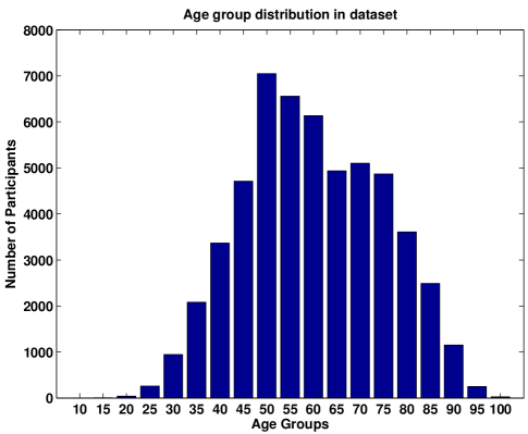
Figure 1: Distribution of age within the patients.

The most common cancer treatment taken by women of white ethnicity is radiotherapy as seen in Figure 2. However this seems to be the least common treatment for women of black African ethnicity.

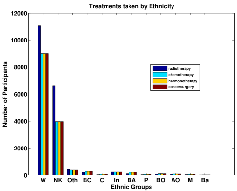
Figure 2: Different treatments for breast cancer.

Figure 3 shows that the women from the white ethnic group are quite evenly distributed in terms of their socioeconomic deprivation.

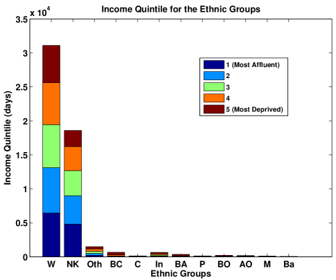
Figure 3: Distribution of income within the patients.

Looking at the average of survival days across the ethnic groups shows that women of Chinese ethnicity have the highest days of survival from breast cancer (see, Figure 4). It also highlights that although the proportion of women of white ethnicity is significantly higher than any other groups, an average count gives a better indication of the caner survival rate across the ethnicity. Figure 7 shows that the proportion of breast cancer survival compared to death is much higher within the white ethnic group and similar in black Caribbean and Indian ethnicity.

Figure 4: Average survival days across the ethnic groups.

III Methodology

III-A Naive Bayes for imputation

In order to fill up the ethnicity of the records with unknown ethnicity group, we decided to take a supervised-learning approach. The supervised-learning (machine learning) uses known set of input data and response to the data to build a predictor model that will generate predictions for the response to the new set of data. Since our dataset mainly consisted of binary and nominal data values we determined that this was a classification problem and chose Naive Bayes classification algorithm to model our predictor. The Naive Bayes algorithm seemed to be the optimal choice despite it having a low predictive accuracy because it handles categorical predictors very well and its speed and memory usage are good for simple distributions. More importantly this algorithm is easy to interpret because it is based on finding the posterior probability for the new data belonging to the classes given that the features are independent of one another in each class.

The Naive Bayes classifier involves two stages. The first stage is training, where the probabilities of every features’ parameter given each class as well as the probability of each class are estimated. These are known as the Likelihood $P(X|C)$ and Class Prior probability $P(C)$ respectively. The second stage is prediction, where the posterior probability algorithm (Eq. 1) calculates the probability of each class given the parameters of each feature in the new data. Finally it predicts the class with the highest posterior probability as the result. As the features of our dataset are also assumed to be independent of each other and the class we believe that using the Naive Bayes algorithm will give us the best output.

$$P(C|X)=\frac{P(X|C)P(C)}{P(X)}.$$ (1)

III-B Parameter tuning

The Naive Bayes Classifier supports a number of probability distribution estimates. Based on theory the Multivariate Multinomial Distribution is the ideal distribution for us to choose as our dataset consists of categorical features; however we decided to conduct a set of parameter tuning experiments with the different distribution options available in Matlab to observe the legitimacy of the theory. We chose: 1)Normal (Gaussian), 2) Kernel, 3) Multinomial and 4) Multivariate Multinomial and set the class prior probability as uniform for all cases so that the probabilities are equal for all classes. subsequently, we decided to choose the best distribution depending on the highest value for accuracy after cross validations.

III-C Cross validation

In order to run the cross validation we first extracted the records of unknown ethnic group from the original dataset and created the training data with the remaining records. We decided to use the K Fold Cross validation process in order to enhance the accuracy of the results and a value of 10 for K seemed ideal for such a large dataset. The 10 fold cross validation involved dividing our training data into 10 sets, then setting aside one set for validation we used the remaining 9 sets to train the Bayesian classifier. Then we cross validated the results with the validation set and calculated its accuracy using unbiased F-measure [16]. This cross validation was computed 10 times where every time a different set was used for validation and then an average of the F-measure percentages are calculated. After running this for each of the distribution parameters we chose to use the distribution with the highest accuracy. We ran the prediction model for the four distributions we considered.

III-D Performance evaluation

The F-measure is a good way to calculate the performance of a prediction model by checking the predicted results against the actual results. The process involves finding the total number of True Positives (tp), True Negatives (tn), False Positives (fp) and False Negatives (fn) from the result comparison. Then finding the Precision and Recall using the equations in Table III where Precision is the ratio of number of correct results to the number of all returned results and Recall is the ratio of the number of correct results to the number of results that should have been returned [11]. Finally the unbiased F-measure is then calculated by finding the harmonic mean of the Precision and Recall rates.

TABLE III: Performance measurement methods

Method	Formula
Recall	$Re=\frac{TP}{TP+FN}$
Precision	$Pr=\frac{TP}{TP+FP}$
F-measure	$F=2*\frac{Pr\times Re}{Pr+Re}$

III-E Imputation

Once the dataset was finally ready to be classified by the Bayesian model we assigned the previously extracted records of the unknown ethnic group as our testing dataset and keeping all of the remaining data records for training and the Ethnic group feature was assigned as the class label. The testing dataset consisted of 18595 records which is around 35% of the original records. This actually gives a close 30:70 ratio between the testing and training which is optimal as previously mentioned. Once the predicted results were obtained we integrated the unknown records back into the original dataset and replaced the unknown values with the predicted ethnic groups.

IV Results

In this section, we present the results for the following:

• Cross validation results for considered distributions.

• Show the effect of ethnicity on the survival rate.

• Show the impact of age on the survival rate.

• Show the implication between financial status and the survival rate.

IV-A Cross validation

Table IV indicates that fitting the Bayesian model with a ’Kernel’ distribution with uniform prior and ’Gaussian’ distribution with no prior as parameters give the most accurate 94.10% and 94.01% results respectively when compared to the other distributions. Therefore, we consider predictions based on kernel distribution for the imputation.

TABLE IV: F-measure % according to each distribution.

Distribution type	F-measure %
Gaussian with no prior	94.01%
Gaussian with uniform prior	48.7%
Kernel with uniform prior	94.10%
Multinomial with uniform prior	41.98%
Multinomial Multivariate with uniform prior	50.80%

IV-B Ethnic groups vs survival rates

IV-B1 Before imputation

Figure 5 shows the distribution of ethnicity within our original dataset. According to that, the majority of our samples are white women (58%). A high percentage (35%) of the samples are from unknown ethnic groups. Other ethnic groups exist in small percentages with Bangladesh being the lowest. The high number of white women is due to socio-demographic reasons. The data was collected in Southwest of England where most of the population is of white ethnic group. This is justified by the data produced by the Office for National Statistics census data, UK [17]. The population in South East England by ethnic group in 2009 contains 90.7% of white ethnicity.

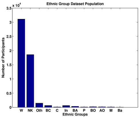
Figure 5: Distribution of ethnic groups with the majority of participants being white.

The distribution of data affects our results due to the unequal number of samples between the ethnic groups. In order to avoid that, we convert the existing numbers to percentages so as to make results more reliable.

The results for the mortality rate according to ethnicity show that the highest number of people that died of breast cancer is in white ethnic group (Figure 5). This does not necessarily mean that this group is more probable to die from breast cancer. In order to get the possibility of each ethnic group facing cancer we translate our results in percentages within each group.

Figure 6: Distribution of ethnic groups with the majority of participants being white.

Figure 6 shows that white women have lower mortality rate than black African, mixed and black other.

IV-B2 After imputation

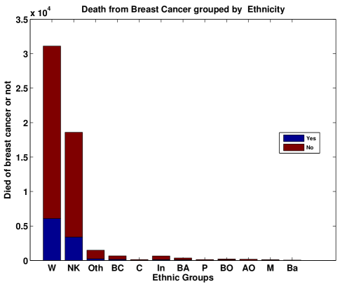
Figure 7: Death and Survival from breast cancer across ethnic groups.

Figure 8 shows the predicted values for the unknown ethnicity records and indicates that the majority of them belong to the white ethnic group.

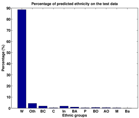
Figure 8: Percentage of predicted data for each ethnicity.

Figure 9 depicts, ‘For women aged between 15-64, the percentage of survival from Breast Cancer of those of white ethnicity is likely to be higher than those of black ethnicity’ as the white women are shown to have a 84% survival rate compared to a 77% survival rate for the women belonging to the Black ethnic group.

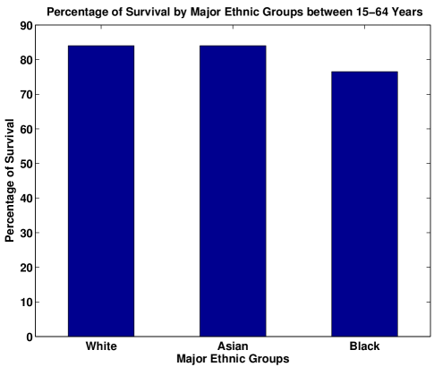
Figure 9: Percentage of survival rate in white is higher than black ethnicity.

Figure 7 and Figure 10 shows the comparison between the ethnic group distribution before and after prediction, respectively where all unknown records are classified into the existing ethnic groups based on the predicted percentages obtained for each ethnicity, as shown in Figure 8. Similarly the comparison of numerals before and after imputation is shown in Table V.

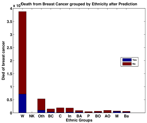
Figure 10: Death from Breast Cancer grouped by Ethnicity after prediction.

IV-C Age vs survival rates

Similarly, we produce the results for the relationship between ages and mortality.

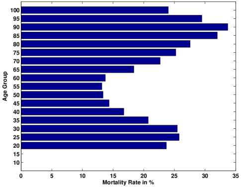
Figure 11: Mortality rate according to age groups.

Figure 11 depicts that ages from 50 to 60 had the lowest possibility of dying from breast cancer. The highest death possibilities are detected in the ages between 80 and 95. Another interesting information is that high death possibilities are detected in the earlier ages of 20-35. This might be because younger people are not properly informed or do not visit their doctors in a frequent basis in comparison to older women.

IV-D Income vs survival rate

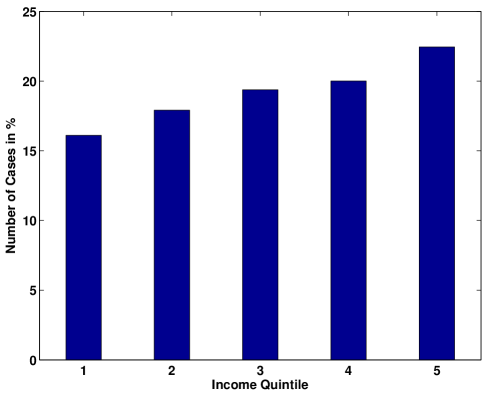
Figure 12: Distribution of income within the patients.

The final objective that we are interested is know whether the financial status effects the death rate. Income feature indicates the financial status of patients and values from 1(richest) to 5(poorer) are used. In Figure 12, we see that wealthier patients have lower death rates. This is probably because they can afford better treatment facilities.

TABLE V: comparison between the ethnic group distribution before and after imputation.

	With Missing data		After Prediction
Ethnicity	Death	Survival	Death	Survival
White	6072.00	25037.00	7184.00	31578.00
Not Known	3385.00	15210.00	0	0
Any Other	230.00	1249.00	986.00	4358.00
Black Caribbean	145.00	507.00	324.00	1156.00
Chinese	14.00	103.00	140.00	1770.00
Indian	113.00	526.00	260.00	1576.00
Black African	95.00	249.00	274.00	595.00
Pakistani	23.00	98.00	92.00	376.00
Black Other	54.00	158.00	147.00	463.00
Asian Other	22.00	148.00	68.00	878.00
Mixed	30.00	83.00	470.00	234.00
Bangladeshi	9.00	33.00	223.00	345.00

V Conclusions and Discussions

After obtaining and appraising our results, we affirm that the type of dataset to be classified plays a role in selecting the appropriate distribution type for the Bayesian classifier. Based on our results, kernel distribution has the best F-measure percentage amongst all other distributions.

Comparing our results with previous statistical research in [18] and [5], we can confirm that our scientific objectives are consistent with their findings. In fact, referring to [6]and [18] approves that white women have higher survival percentage than black women with 91.4% and 85%, respectively. Similarly, older woman and lower income groups have high mortality rates.

There always exists some limitations with the data collection. In fact, by examining the breast cancer dataset, we can notice a clear imbalanced number of participants between the different ethnic groups where white females were representing more than half of the population versus very few numbers amongst all other ethnicity. This limitation might have certainly misled our prediction results which may explain the low F-measure percentages obtained on other distributions excluding kernel and Gaussian.

References

- [1] C. L. Griffiths and J. L. Olin, “Triple negative breast cancer: a brief review of its characteristics and treatment options,” Journal of pharmacy practice, vol. 25, no. 3, pp. 319–323, 2012.
- [2] J. W. Eley, H. A. Hill, V. W. Chen, D. F. Austin, M. N. Wesley, H. B. Muss, R. S. Greenberg, R. J. Coates, P. Correa, C. K. Redmond et al., “Racial differences in survival from breast cancer: results of the national cancer institute black/white cancer survival study,” Jama, vol. 272, no. 12, pp. 947–954, 1994.
- [3] V. Grann, A. B. Troxel, N. Zojwalla, D. Hershman, S. A. Glied, and J. S. Jacobson, “Regional and racial disparities in breast cancer-specific mortality,” Social science & medicine, vol. 62, no. 2, pp. 337–347, 2006.
- [4] S. L. Parker, K. J. Davis, P. A. Wingo, L. A. Ries, and C. W. Heath, “Cancer statistics by race and ethnicity,” CA: a cancer journal for clinicians, vol. 48, no. 1, pp. 31–48, 1998.
- [5] C. J. Bradley, C. W. Given, and C. Roberts, “Race, socioeconomic status, and breast cancer treatment and survival,” Journal of the National Cancer Institute, vol. 94, no. 7, pp. 490–496, 2002.
- [6] R. J, “Cancer incidence and survival by major ethnic group, england, 2002 - 2006,” Cancer Research UK, 2009, [Online; accessed 19-May-2014].
- [7] D. B. Rubin, Multiple imputation for nonresponse in surveys. John Wiley & Sons, 2004, vol. 81.
- [8] J. M. Brick and G. Kalton, “Handling missing data in survey research,” Statistical methods in medical research, vol. 5, no. 3, pp. 215–238, 1996.
- [9] J. L. Schafer, “Multiple imputation: a primer,” Statistical methods in medical research, vol. 8, no. 1, pp. 3–15, 1999.
- [10] R. J. Little and D. B. Rubin, “Statistical analysis with missing data,” 2002.
- [11] B. G. Tabachnick, L. S. Fidell et al., “Using multivariate statistics,” 2001.
- [12] P. D. Allison, “Missing data: Quantitative applications in the social sciences,” British Journal of Mathematical and Statistical Psychology, vol. 55, no. 1, pp. 193–196, 2002.
- [13] S. Sethi and M. E. Seligman, “Optimism and fundamentalism,” Psychological Science, vol. 4, no. 4, pp. 256–259, 1993.
- [14] D. C. Hoaglin and R. E. Welsch, “The hat matrix in regression and anova,” The American Statistician, vol. 32, no. 1, pp. 17–22, 1978.
- [15] D. Lowd and P. Domingos, “Naive bayes models for probability estimation,” in Proceedings of the 22nd international conference on Machine learning. ACM, 2005, pp. 529–536.
- [16] G. Forman and M. Scholz, “Apples-to-apples in cross-validation studies: pitfalls in classifier performance measurement,” ACM SIGKDD Explorations Newsletter, vol. 12, no. 1, pp. 49–57, 2010.
- [17] CODE, “The center for dynamics of ethnicity,” ethnicity.ac.uk, 2009, [Online; accessed 10-May-2014].
- [18] R. Jack, E. Davies, and H. Møller, “Breast cancer incidence, stage, treatment and survival in ethnic groups in south east england,” British journal of cancer, vol. 100, no. 3, pp. 545–550, 2009.