The Cosmological Constant as an Eigenvalue of the Hamiltonian constraint in a Varying Speed of Light theory

Abstract

In the framework of a Varying Speed of Light theory, we study the eigenvalues associated with the Wheeler-DeWitt equation representing the vacuum expectation values associated with the cosmological constant. We find that the Wheeler-DeWitt equation for the Friedmann-Lemaître-Robertson-Walker metric is completely equivalent to a Sturm-Liouville problem provided that the related eigenvalue and the cosmological constant be identified. The explicit calculation is performed with the help of a variational procedure with trial wave functionals related to the Bessel function of the second kind $K_{\nu}\left(x\right)$. We find the existence of a family of eigenvalues associated to a negative power of the scale. Furthermore, we show that at the inflationary scale such a family of eigenvalues does not appear.

I Introduction

What is the Cosmological Constant? How can be computed? These are some of the many puzzling questions which are still unsolved. Basically the Cosmological Constant can be connected to the energy of the vacuum. However, the absence of a complete Quantum Gravitational theory increases the number of questions instead of giving answers. General Relativity (GR) is the best theory explaining the behavior of the gravitational field including also the cosmological constant. However GR fails to describe the gravitational field in the quantum range. Despite of this problem, in GR there exists a quantization procedure known as the Wheeler-De Witt equation (WDW)DeWitt which encodes some aspects of the quantum properties of the gravitational field included the cosmological constant. We say “some”, because a complete solution of the WDW equation does not exist and one needs to reduce the degree of the difficulty by fixing a background and freezing some degrees of freedom. The WDW equation is the quantum version of the classical Hamiltonian constraint representing the invariance under time reparametrization. Its derivation is a consequence of the Arnowitt-Deser-Misner (ADM) decomposition ADM of space time based on the following line element

$$ds^{2}=g_{\mu\nu}\left(x\right)dx^{\mu}dx^{\nu}=\left(-N^{2}+N_{i}N^{i}\right)dt^{2}+2N_{j}dtdx^{j}+g_{ij}dx^{i}dx^{j},$$ (1)

where $N$ is the lapse function and $N_{i}$ the shift function. In terms of the ADM variables, the four dimensional scalar curvature $R$ can be decomposed in the following way

$$\mathcal{R}=R+K_{ij}K^{ij}-\left(K\right)^{2}-2\nabla_{\mu}\left(Ku^{\mu}+a^{\mu}\right),$$ (2)

where

$$K_{ij}=-\frac{1}{2N}\left[\partial_{t}g_{ij}-N_{i|j}-N_{j|i}\right]$$ (3)

is the second fundamental form, $K=$ $g^{ij}K_{ij}$ is its trace, $R$ is the three dimensional scalar curvature and $\sqrt{g}$ is the three dimensional determinant of the metric. The last term in $\left(\ref{R}\right)$ represents the boundary terms contribution where the four-velocity $u^{\mu}$ is the timelike unit vector normal to the spacelike hypersurfaces ($t$=constant) denoted by $\Sigma_{t}$ and $a^{\mu}=u^{\alpha}\nabla_{\alpha}u^{\mu}$ is the acceleration of the timelike normal $u^{\mu}$. Thus

$$\mathcal{L}\left[N,N_{i},g_{ij}\right]=\sqrt{-\text{\/\thinspace\thinspace}^{4}\text{\/{}\negthinspace}g}\left(\mathcal{R}-2\Lambda\right)=\frac{N}{2\kappa}\sqrt{g}\text{ }\left[K_{ij}K^{ij}-K^{2}+\,R-2\Lambda-2\nabla_{\mu}\left(Ku^{\mu}+a^{\mu}\right)\right]$$ (4)

represents the gravitational Lagrangian density where $\kappa=8\pi G$ with $G$ the Newton’s constant and for the sake of generality we have also included a cosmological constant $\Lambda$. After a Legendre transformation, the WDW equation simply becomes

$$\mathcal{H}\Psi=\left[\left(2\kappa\right)G_{ijkl}\pi^{ij}\pi^{kl}-\frac{\sqrt{g}}{2\kappa}\!{}\!\left(\,\!R-2\Lambda\right)\right]\Psi=0,$$ (5)

where $G_{ijkl}$ is the super-metric and where the conjugate super-momentum $\pi^{ij}$ is defined as

$$\pi^{ij}=\frac{\delta\mathcal{L}}{\delta\left(\partial_{t}g_{ij}\right)}=\left(g^{ij}K-K^{ij}\text{ }\right)\frac{\sqrt{g}}{2\kappa}.$$ (6)

Note that $H=0$, represents the classical constraint which guarantees the invariance under time reparametrization. The other classical constraint represents the invariance by spatial diffeomorphism and it is described by $\pi_{|j}^{ij}=0$, where the vertical stroke “$|$” denotes the covariant derivative with respect to the $3D$ metric $g_{ij}$. Solving Eq.$\left(\ref{WDWO}\right)$ allows to extract information on the early universe and on the cosmological constant. Of course, the form of the solution is depending on the background one considers. In this paper, we fix our attention on the Friedmann-Lemaître-Robertson-Walker (FLRW) metric without matter fields. To the reader, this choice could seem a restriction, however one has to think that in the very early universe, before the inflationary phase, it is likely that all the quantum information can be carried on by the gravitational field, because of its non-linear nature. However, even in this simplified vision many problems arise, especially for the inflationary epoch. In recent years, the idea of modifying GR to cure some of its diseases has been considered. From one side, the so-called $f\left(R\right)$ theories have been taken under examination to cure some problems in the infrared (IR) regionf(R) and on the other hand modifications on short scales allowing a power-counting ultraviolet (UV) renormalizable have been proposed by Hořava motivated by the Lifshitz theory in solid state physicsHorava Lifshitz . This theory is dubbed as Hořava-Lifshitz (HL) theory and should recover general relativity in the IR limit. Nevertheless the price to pay to obtain a renormalizable theory in the HL proposal is that we have no general covariance or, in other words Lorentz symmetry is broken. Another proposal which distorts gravity in the UV is Gravity’s RainbowMagSmo . Gravity’s Rainbow has some appealing features to explain inflationAM . In a series of papers, one of us used Gravity’s Rainbow to cure some divergences appearing in Zero Point Energy (ZPE) calculations, at least to one loopGMLM . The final ZPE result has been interpreted as an induced Cosmological Constant obtained as an eigenvalue of an appropriate Sturm-Liouville problem. It is interesting to note that the same idea has been applied in a HL theoryRemoHL in a FLRW background, the final result is that non trivial eigenvalues have been found depending on the parameters of the theory. Note that in GR, as we will show extensively in the next section, the cosmological constant cannot be considered as an eigenvalue of any Sturm-Liouville problem for the FLRW background in a mini-superspace approximation without matter fields. It appears therefore, that distortions of GR allow new results that otherwise should not be possible. It remains to consider another distortion connected with the previous ones: a Varying Speed of Light (VSL) theoryharko ; moffat ; Albrecht ; Barrow1 ; Barrow2 ; Barrow3 . In this approach, one allows the speed of light to change in some specified way, in an attempt to solve the major cosmological issues of modern theoretical physics. It is well known, that one of the major features of Einstein’s theory of relativity is that the speed of light in a vacuum is always at constant rate. However, the cosmological problems that led to the theoretical introduction of dark matter and dark energy into modern cosmology have motivated some physicists to look for solutions in other directions, included the variation of the speed of light. In VSL, it is supposed that light travels faster in the early periods of the existence of the Universe and for this reason, it could solve problems related to the inflationary phase (flatness, horizon, homogeneity, etc.…)Barrow1 Kolb90 ; guth ; linde ; AA ; veneziano . Of course, this hypothesis breaks the Lorentz invariance. The VSL model has been embedded within the general framework of the time varying fine structure constant theory and reformulated as a dielectric vacuum theory Barrow2 . Moreover, isotropy and homogeneity problems may find their appropriate solutions through this mechanism ellis ; magueio ; moff . Recently quantum cosmological aspect of VSL models have been studied to see if the “Tunneling from Nothing”Vilenkin  and the “Hartle-Hawking No-boundary proposal”HH  can be better approached in this contextharko1 ; sho . The purpose of this paper is to repeat the calculation of Ref.RemoHL in a VSL context to see if there are non trivial eigenvalues of an appropriate Sturm-Liouville problem, which will be interpreted as a Cosmological Constant induced by quantum fluctuations of the scale factor. The paper is organized as follows. In Sec. II we discuss the Wheeler-deWitt equations for Friedmann-Lemaître-Robertson-Walker space time. While, in Sec. III, we show how it is possible to derive the Wheeler-deWitt equations for Friedmann-Lemaître-Robertson-Walker space time in presence of varying speed of light. Conclusions are drawn in Sec.IV.

II The Wheeler-DeWitt equation for the Friedmann-Lemaître-Robertson-Walker space-time

A homogeneous, isotropic and closed universe is represented by the FLRW line element

$$ds^{2}=-N^{2}dt^{2}+a^{2}\left(t\right)d\Omega_{3}^{2},$$ (7)

where

$$d\Omega_{3}^{2}=\gamma_{ij}dx^{i}dx^{j}$$ (8)

is the line element on the three-sphere, $N$ is the lapse function and $a(t)$ denotes the scale factor. Let us consider a very simple mini-superspace model described by the metric of Eq.$\left(\ref{FRW}\right)$. In this background, the Ricci curvature tensor and the scalar curvature read simply

$$R_{ij}=\frac{2}{a^{2}\left(t\right)}\gamma_{ij}\qquad\mathrm{and}\qquad R=\frac{6}{a^{2}\left(t\right)}~{},$$ (9)

respectively. The Einstein-Hilbert action in $(3+1)$-dim is

$$S=\frac{1}{16\pi G}\int_{\Sigma\times I}\mathcal{L}~{}dt~{}d^{3}x=\frac{1}{16\pi G}\int_{\Sigma\times I}N\sqrt{g}\left[K^{ij}K_{ij}-K^{2}+R-2\Lambda\right]~{}dt~{}d^{3}x~{},$$ (10)

with $\Lambda$ the cosmological constant, $K_{ij}$ the extrinsic curvature and $K$ its trace. Using the line element, Eq. $\left(\ref{FRW}\right)$, the above written action, Eq. $\left(\ref{action}\right)$, becomes

$$S=-\frac{3\pi}{4G}\int_{I}\left[\dot{a}^{2}a-a+\frac{\Lambda}{3}a^{3}\right]dt~{},$$ (11)

where we have computed the volume associated to the three-sphere, namely $V_{3}=2\pi^{2}$, and set $N=1$.

The canonical momentum reads

$$\pi_{a}=\frac{\delta S}{\delta\dot{a}}=-\frac{3\pi}{2G}\dot{a}a~{},$$ (12)

and the resulting Hamiltonian density is

$$\mathcal{H} =\pi_{a}\dot{a}-\mathcal{L}$$

$$=-\frac{G}{3\pi a}\pi_{a}^{2}-\frac{3\pi}{4G}a+\frac{3\pi}{4G}\frac{\Lambda}{3}a^{3}~{}.$$ (13)

Following the canonical quantization prescription, we promote $\pi_{a}$ to a momentum operator, setting

$$\pi_{a}^{2}\rightarrow-a^{-q}\left[\frac{\partial}{\partial a}a^{q}\frac{\partial}{\partial a}\right],$$ (14)

where we have introduced a factor order ambiguity $q$. The generalization to $k=0,-1$ is straightforward. The WDW equation for such a metric is

$$H\Psi\left(a\right)=\left[-a^{-q}\left(\frac{\partial}{\partial a}a^{q}\frac{\partial}{\partial a}\right)+\frac{9\pi^{2}}{4G^{2}}\left(a^{2}-\frac{\Lambda}{3}a^{4}\right)\right]\Psi\left(a\right)\,,$$

$$\left[-\frac{\partial^{2}}{\partial a^{2}}-\frac{q}{a}\frac{\partial}{\partial a}+\frac{9\pi^{2}}{4G^{2}}\left(a^{2}-\frac{\Lambda}{3}a^{4}\right)\right]\Psi\left(a\right)=0.$$ (15)

It represents the quantum version of the invariance with respect to time reparametrization. If we define the following reference length $a_{0}=\sqrt{3/\Lambda}$, then Eq.$\left(\ref{WDW_0}\right)$ assumes the familiar form of a one-dimensional Schrödinger equation for a particle moving in the potential

$$U\left(a\right)=\frac{9\pi^{2}a_{0}^{2}}{4G^{2}}\left[\left(\frac{a}{a_{0}}\right)^{2}-\left(\frac{a}{a_{0}}\right)^{4}\right]\,,$$ (16)

with zero total energy. The potential $U\left(a\right)$ resembles a potential well which is unbounded from below. When $0<a<a_{0}$, Eq. $\left(\ref{U(a)}\right)$ implies $U\left(a\right)>0$, which is the classically forbidden region, while for $a>a_{0}$, one gets $U\left(a\right)<0$, which is the classically allowed region. It is interesting to note that for for the special case of the operator ordering $q=-1$, one can determine exact solutionVilenkin . This can be easily verified by introducing the function

$$z\left(a\right)=\left(\frac{3\pi a_{0}^{2}}{4G}\right)^{\frac{2}{3}}\left(1-\frac{a^{2}}{a_{0}^{2}}\right)=z_{0}\left(1-\frac{a^{2}}{a_{0}^{2}}\right),$$

where the solution can be written in terms of Airy functions, namely

$$\Psi\left(a\right)=\alpha Ai\left(z\right)+\beta Bi\left(z\right).$$ (17)

However, the wave function $\left(\ref{Airy}\right)$, cannot be normalized in the following sense

$$\int_{0}^{\infty}daa^{q}\Psi^{\ast}\left(a\right)\Psi\left(a\right).$$ (18)

The same happens for the other special value $q=3$. Even if the WDW equation $\left(\ref{WDW_0}\right)$ has a zero energy eigenvalue, it also has a hidden structure. Indeed Eq.$\left(\ref{WDW_0}\right)$ has the structure of a Sturm-Liouville eigenvalue problem with the cosmological constant as eigenvalue. We recall to the reader that a Sturm-Liouville differential equation is defined by

$$\frac{d}{dx}\left(p\left(x\right)\frac{dy\left(x\right)}{dx}\right)+q\left(x\right)y\left(x\right)+\lambda w\left(x\right)y\left(x\right)=0$$ (19)

and the normalization is defined by

$$\int_{a}^{b}dxw\left(x\right)y^{\ast}\left(x\right)y\left(x\right).$$ (20)

In the case of the FLRW model we have the following correspondence

$$p\left(x\right) \rightarrow a^{q}\left(t\right)\,,$$

$$q\left(x\right) \rightarrow\left(\frac{3\pi}{2G}\right)^{2}a^{q+2}\left(t\right)\,,$$

$$w\left(x\right) \rightarrow a^{q+4}\left(t\right)\,,$$

$$y\left(x\right) \rightarrow\Psi\left(a\right)\,,$$

$$\lambda \rightarrow\frac{\Lambda}{3}\left(\frac{3\pi}{2G}\right)^{2}\,,$$ (21)

and the normalization becomes

$$\int_{0}^{\infty}daa^{q+4}\Psi^{\ast}\left(a\right)\Psi\left(a\right).$$ (22)

It is a standard procedure, to convert the Sturm-Liouville problem $\left(\ref{SL}\right)$ into a variational problem of the form

$$F\left[y\left(x\right)\right]=\frac{-\int_{a}^{b}dxy^{\ast}\left(x\right)\left[\frac{d}{dx}\left(p\left(x\right)\frac{d}{dx}\right)+q\left(x\right)\right]y\left(x\right)}{\int_{a}^{b}dxw\left(x\right)y^{\ast}\left(x\right)y\left(x\right)}\,.$$ (24)

with boundary condition to be specified. If $y\left(x\right)$ is an eigenfunction of $\left(\ref{SL}\right)$, then

$$\lambda=\frac{-\int_{a}^{b}dxy^{\ast}\left(x\right)\left[\frac{d}{dx}\left(p\left(x\right)\frac{d}{dx}\right)+q\left(x\right)\right]y\left(x\right)}{\int_{a}^{b}dxw\left(x\right)y^{\ast}\left(x\right)y\left(x\right)}\,,$$ (25)

is the eigenvalue, otherwise

$$\lambda_{1}=\min_{y\left(x\right)}\frac{-\int_{a}^{b}dxy^{\ast}\left(x\right)\left[\frac{d}{dx}\left(p\left(x\right)\frac{d}{dx}\right)+q\left(x\right)\right]y\left(x\right)}{\int_{a}^{b}dxw\left(x\right)y^{\ast}\left(x\right)y\left(x\right)}\,.$$ (26)

The minimum of the functional $F\left[y\left(x\right)\right]$ corresponds to a solution of the Sturm-Liouville problem $\left(\ref{SL}\right)$ with the eigenvalue $\lambda.$ In the mini-superspace approach with a FLRW background, one finds RemoHL

$$\frac{\int\mathcal{D}aa^{q}\Psi^{\ast}\left(a\right)\left[-\frac{\partial^{2}}{\partial a^{2}}-\frac{q}{a}\frac{\partial}{\partial a}+\frac{9\pi^{2}}{4G^{2}}a^{2}\right]\Psi\left(a\right)}{\int\mathcal{D}aa^{q+4}\Psi^{\ast}\left(a\right)\Psi\left(a\right)}=\frac{3\Lambda\pi^{2}}{4G^{2}},$$ (27)

The best form of the trial wave function can be guessed by looking the asymptotic behavior of Eq.$\left(\ref{WDW_0}\right)$. For $a\rightarrow\infty$, we find

$$\left[-\frac{\partial^{2}}{\partial a^{2}}-\frac{q}{a}\frac{\partial}{\partial a}+\frac{9\pi^{2}}{4G^{2}}\left(a^{2}-\frac{\Lambda}{3}a^{4}\right)\right]\Psi\left(a\right)\simeq\left[-\frac{\partial^{2}}{\partial a^{2}}-\frac{3\Lambda\pi^{2}}{4G^{2}}a^{4}\right]\Psi\left(a\right)=0$$ (28)

and when $a\rightarrow 0$, we find

$$\left[-\frac{\partial^{2}}{\partial a^{2}}-\frac{q}{a}\frac{\partial}{\partial a}+\frac{9\pi^{2}}{4G^{2}}\left(a^{2}-\frac{\Lambda}{3}a^{4}\right)\right]\Psi\left(a\right)\simeq\left[-\frac{\partial^{2}}{\partial a^{2}}-\frac{q}{a}\frac{\partial}{\partial a}+\frac{9\pi^{2}}{4G^{2}}a^{2}\right]\Psi\left(a\right)=0.$$ (29)

When $a\rightarrow 0$, the previous equation can be exactly solved by a superposition of modified Bessel functions of the first $\left(I_{\nu}\left(x\right)\right)$ and second kind $\left(K_{\nu}\left(x\right)\right)$. We findWiltshire

$$\Psi_{0}\left(a\right)=C_{1}{a}^{\left(1-q\right)/2}I_{\left(q-1\right)/4}{\left(\frac{3\pi}{4G}{a}^{2}\right)}+C_{2}{a}^{\left(1-q\right)/2}K_{\left(q-1\right)/4}{\left(\frac{3\pi}{4G}{a}^{2}\right).}$$ (30)

However, the solution $\left(\ref{sol}\right)$ is exact for a vanishing eigenvalue. Since our purpose is the evaluation of Eq.$\left(\ref{WDW_1}\right)$, we need a solution for $a\rightarrow 0$, which considers a generic not vanishing eigenvalue. This is described by

$$\Psi\left(a\right)=C_{1}\exp\left(-\frac{3\pi a^{2}}{8G}\right)M{\left(\frac{q+1}{4}-\frac{GE^{2}}{3\pi},\frac{q+1}{2},\frac{3\pi}{4G}{a}^{2}\right)}$$

$$+C_{2}\exp\left(-\frac{3\pi a^{2}}{8G}\right)U{\left(\frac{q+1}{4}-\frac{GE^{2}}{3\pi},\frac{q+1}{2},\frac{3\pi}{4G}{a}^{2}\right),}$$ (31)

where $M{\left(a,b,x\right)}$ and $U{\left(a,b,x\right)}$ are the Kummer functions. For practical purposes, it is useful to transform $M{\left(a,b,x\right)}$ and $U{\left(a,b,x\right)}$ in terms of $I_{\nu}\left(x\right)$ and $K_{\nu}\left(x\right)$. We find

$$\left\{\begin{array}[c]{c}M{\left(a+1/2,2a+1,2x\right)=\Gamma}\left(1+a\right)\mathrm{\exp}\left(x\right)I_{a}{\left(x\right)/}\left(x/2\right)^{a}\\ \\ U{\left(a+1/2,2a+1,2x\right)=}\mathrm{\exp}\left(x\right)K_{a}{\left(x\right)/}\left(\sqrt{\pi}\left(2x\right)^{a}\right)\end{array}\right..$$ (32)

Since $M{\left(a,b,x\right)}$ is proportional to $I_{a}{\left(x\right)}$ which is divergent for large $x$, we will fix $C_{1}=0$ to obtain normalizable solutions. Thus, we consider the following form

$$\Psi\left(a\right)=\exp\left(-\frac{\beta{a}^{2}}{2}\right)U{\left(\frac{q+1}{4},\frac{q+1}{2},\beta{a}^{2}\right)=\frac{\left(\beta{a}^{2}\right)^{\left(1-q\right)/4}}{\sqrt{\pi}}K_{\left(q-1\right)/4}{\left(\frac{\beta{a}^{2}}{2}\right)}},$$ (33)

for the trial wave function and we plug $\left(\ref{Psi}\right)$ into Eq.$\left(\ref{WDW_1}\right)$. After an integration over the scale factor $a\left(t\right)$, one gets

$$\frac{3\Lambda\left(\beta\right)\pi^{2}}{4G^{2}}=\frac{\int_{0}^{\infty}dxxK_{\left(q-1\right)/4}^{2}{\left(x\right)}}{2\int_{0}^{\infty}dxx^{2}K_{\left(q-1\right)/4}^{2}{\left(x\right)}}\left(-\beta^{3}+\frac{9\pi^{2}}{4G^{2}}\beta\right),$$ (34)

where $\beta$ is a variational parameter and where we have rescaled the integrals with the help of the results of Appendix A. By imposing that $\Lambda\left(\beta\right)$ be stationary against arbitrary variations of the parameter $\beta$, we obtain

$$\frac{d}{d\beta}\Lambda\left(\beta\right)=\frac{3\int_{0}^{\infty}dxxK_{\left(q-1\right)/4}^{2}{\left(x\right)}}{2\int_{0}^{\infty}dxx^{2}K_{\left(q-1\right)/4}^{2}{\left(x\right)}}\left(\frac{2G}{3\pi}\right)^{2}\frac{d}{d\beta}\left(-\beta^{3}+\left(\frac{3\pi}{2G}\right)^{2}\beta\right)=\,0.$$ (35)

This implies

$$\beta_{\pm}=\pm\frac{\sqrt{3}\pi}{2G}.$$ (36)

Plugging $\left(\ref{sol12}\right)$ into Eq.$\left(\ref{LambdaB}\right)$, one finds

$$\Lambda\left(\beta_{\pm}\right)=4\beta_{\pm}\frac{\Gamma\left(\frac{3+q}{4}\right)\Gamma\left(\frac{5-q}{4}\right)}{\Gamma\left(\frac{5+q}{4}\right)\Gamma\left(\frac{7-q}{4}\right)}.$$ (37)

It is easy to check that $\beta_{+}$ is a maximum and $\beta_{-}$ is a minimum. However $\beta_{-}$ is negative independently on $q$ and this leads to a normalization $\left(\ref{Norm1}\right)$ in the range $\left(-\infty,0\right]$ which is non physical. A further exploration with a pure Gaussian choice, namely

$$\Psi\left(a\right)=\exp\left(-\frac{\beta{a}^{2}}{2}\right)$$ (38)

for $q=0$, leads to

$$3\Lambda\left(\frac{\pi}{2G}\right)^{2}=\frac{\int\mathcal{D}a\Psi^{\ast}\left(a\right)\left[-\frac{\partial^{2}}{\partial a^{2}}+\left(\frac{3\pi}{2G}\right)^{2}a^{2}\right]\Psi\left(a\right)}{\int\mathcal{D}aa^{4}\Psi^{\ast}\left(a\right)\Psi\left(a\right)}=\frac{2}{3}\left(\beta^{3}+\left(\frac{3\pi}{2G}\right)^{2}\beta\right).$$ (39)

The application of the variational procedure leads to imaginary solutions and therefore it will be discarded. It remains to test the following assumption

$$\Psi\left(a\right)=\exp\left(-\frac{\beta{a}^{4}}{2}\right),$$ (40)

suggested by the asymptotic behavior $\left(\ref{asy}\right)$. In the next section we will discuss the choice $\left(\ref{a4}\right)$ as a particular case of a VSL theory. One could insist in this direction and try to explore other trial wave functions. However, choices $\left(\ref{twf}\right)$, $\left(\ref{Gauss}\right)$ and $\left(\ref{a4}\right)$ have been chosen following the standard procedure for a variational approach. Therefore, the other choices can only be small variations of the proposed trial wave functions above mentioned. Therefore we are led to consider a distorted version of the gravitational field induced by a VSL theory.

III The Wheeler-DeWitt equation for the Friedmann-Lemaitre-Robertson-Walker space-time in the presence of varying speed of light

A VSL cosmology model is described by the following line element

$$ds^{2}=-N^{2}\left(t\right)c^{2}\left(t\right)dt^{2}+a^{2}\left(t\right)d\Omega_{3}^{2},$$ (41)

where $d\Omega_{3}^{2}$ is described by Eq.$\left(\ref{domega}\right)$ and where $c\left(t\right)$ is an arbitrary function of time with the dimensions of a $\left[length/time\right]$. The form of the background is such that the shift function $N^{i}$ vanishes. Thus, the extrinsic curvature reads

$$K_{ij}=-\frac{\dot{g}_{ij}}{2N\left(t\right)c\left(t\right)}=-\frac{\dot{a}\left(t\right)}{N\left(t\right)c\left(t\right)a\left(t\right)}g_{ij},$$ (42)

where the dot denotes differentiation with respect to time $t$. The gravitational action fulfilling the Einstein’s Field equation with the speed of light explicitly written is

$$S=\frac{1}{16\pi G}\int_{\mathcal{M}}c^{4}\left(t\right)\sqrt{-g}Rd^{4}x,$$ (43)

where we have used the following relationship $dx^{0}=c\left(t\right)dt$. It is easy to write the form of the reduced action of the mini-superspace. Indeed, reintroducing the speed of light into the action $\left(\ref{action}\right)$, one gets in $(3+1)$

$$S=\frac{1}{16\pi G}\int_{\Sigma\times I}N\left(t\right)c^{4}\left(t\right)\sqrt{g}\left[K^{ij}K_{ij}-K^{2}+R-2\Lambda\right]~{}dt~{}d^{3}x~{},$$ (44)

Using the line element, Eq. $\left(\ref{FRWc}\right)$, the above written action, Eq. $\left(\ref{actionc}\right)$, becomes

$$S=-\frac{3\pi}{4G}\int_{I}c^{2}\left(t\right)\left[\dot{a}^{2}a-ac^{2}\left(t\right)+\frac{\Lambda}{3}a^{3}c^{2}\left(t\right)\right]dt~{},$$ (45)

where we have computed the volume associated to the three-sphere, namely $V_{3}=2\pi^{2}$, and set $N=1$. The canonical momentum reads

$$\pi_{a}=\frac{\delta S}{\delta\dot{a}}=-\frac{3\pi}{2G}\dot{a}\,a\,c^{2}\left(t\right)~{},$$ (46)

and the resulting Hamiltonian density is

$$\mathcal{H} =\pi_{a}\dot{a}-\mathcal{L}$$

$$=-\frac{G}{3\pi ac^{2}\left(t\right)}\pi_{a}^{2}-\frac{3\pi}{4G}a\,c^{4}\left(t\right)+\frac{3\pi}{4G}\frac{\Lambda}{3}a^{3}c^{4}\left(t\right)~{}.$$ (47)

According to the usual prescription where $\pi_{a}$ is promoted to an operator, we can write

$$\pi_{a}\rightarrow-i\hbar c\left(t\right)\frac{\partial}{\partial a}$$ (48)

and introducing the factor ordering ambiguity

$$\pi_{a}^{2}\rightarrow-\left(\hbar c\left(t\right)\right)^{2}a^{-q}\frac{\partial}{\partial a}a^{q}\frac{\partial}{\partial a},$$ (49)

the WDW equation $\mathcal{H}\Psi=0$ simply becomes

$$\left[-\frac{G}{3\pi ac^{2}\left(t\right)}\pi_{a}^{2}-\frac{3\pi}{4G}a\,c^{4}\left(t\right)+\frac{3\pi}{4G}\frac{\Lambda}{3}a^{3}c^{4}\left(t\right)\right]\Psi\left(a\right)=0.$$ (50)

FollowingBarrow1 ; Barrow2 ; Barrow3 , we assume that

$$c\left(t\right)=c_{0}\left(\frac{a\left(t\right)}{a_{0}}\right)^{\alpha}$$ (51)

where $a_{0}$ is a reference length scale whose value will be fixed later. If the factor ordering is not distorted by the presence of a varying speed of light, one can further simplify the above equation to obtain

$$\left(-\frac{\partial^{2}}{\partial a^{2}}-\frac{q}{a}\frac{\partial}{\partial a}+U_{c}\left(a\right)\right)\Psi\left(a\right)=0,$$ (52)

where we have set $N=1$ and the quantum potential is defined as

$$U_{c}\left(a\right)=\left(\frac{3\pi}{2G\hbar}\right)^{2}a^{2}c^{6}\left(t\right)\left(1-\frac{\Lambda}{3}a^{2}\right)=\left(\frac{3\pi c_{0}^{3}}{2G\hbar a_{0}^{3\alpha}}\right)^{2}a^{2+6\alpha}\left(1-\frac{\Lambda}{3}a^{2}\right).$$ (53)

Note that the potential $U_{c}\left(a\right)$ vanishes in the same points where $U\left(a\right)$ has its roots. Now, we are ready to discuss the analogue of Eq.$\left(\ref{WDW_1}\right)$ in presence of a VSL distortion. To this purpose Eq.$\left(\ref{WDWg}\right)$ can be cast into the form

$$\frac{\int\mathcal{D}aa^{q}\Psi^{\ast}\left(a\right)\left[-\frac{\partial^{2}}{\partial a^{2}}-\frac{q}{a}\frac{\partial}{\partial a}+\left(\frac{3\pi}{2l_{P}^{2}a_{0}^{3\alpha}}\right)^{2}a^{2+6\alpha}\right]\Psi\left(a\right)}{\int\mathcal{D}aa^{q+4+6\alpha}\Psi^{\ast}\left(a\right)\Psi\left(a\right)}=3\Lambda\left(\frac{\pi}{2l_{P}^{2}a_{0}^{3\alpha}}\right)^{2},$$ (56)

where we have defined $l_{P}=\sqrt{G\hbar/c_{0}^{3}}$. Because of the VSL distortion, the asymptotic behavior of the trial wave function must be different compared to $\left(\ref{WDW_1}\right)$. Since

$$\left\{\begin{array}[c]{cc}K_{\nu}{\left(x\right)\rightarrow}\sqrt{\pi/\left(2x\right)}\mathrm{\exp}\left(-x\right)&x\rightarrow\infty\\ &\\ \begin{array}[c]{c}K_{0}{\left(x\right)\rightarrow-\ln}\left(x\right)\\ K_{\nu}{\left(x\right)\rightarrow}\Gamma\left(\nu\right)\left(x/2\right)^{-\nu}/2\end{array}&x\rightarrow 0\end{array}\right.,$$ (57)

we find extremely useful the following assumption of the trial wave function

$$\Psi\left(a\right)={a}^{-\frac{q+1}{2}}\left(\beta{a}\right)^{-3\alpha}\exp\left(-\frac{\beta{a}^{4}}{2}\right),$$ (58)

which is a small variation of $\left(\ref{Psi}\right)$. The exponential encodes the large $a$ behavior, while $\left(\beta{a}\right)^{-3\alpha}$ encodes the small scale factor behavior and $\beta$ is the variational parameter. Plugging $\left(\ref{Psib}\right)$ into Eq.$\left(\ref{VeV}\right)$, after an integration over the scale factor $a\left(t\right)$, we find

$$\Lambda_{q,\alpha}\left(\beta\right)=3\left(\frac{2l_{P}^{2}a_{0}^{3\alpha}}{3\pi}\right)^{2}\left(C_{q}\left(\alpha\right){{\beta}^{\frac{3\left(1+\alpha\right)}{2}}}+\left(\frac{3\pi}{2l_{P}^{2}a_{0}^{3\alpha}}\right)^{2}\sqrt{{{\beta\pi}}}\right),$$ (59)

where

$$C_{q}\left(\alpha\right)=\frac{1}{4}{({q}^{2}-24\alpha-2\,q-7)\Gamma\left({-\frac{1+3{\alpha}}{2}}\right)}.$$ (60)

We demand that

$$\frac{d\Lambda_{q,\alpha}\left(\beta\right)}{d\beta}=\frac{3}{2{{\beta}^{\frac{1}{{2}}}}}\left(\frac{2l_{P}^{2}a_{0}^{3\alpha}}{3\pi}\right)^{2}\left(3\left(1+\alpha\right)C_{q}\left(\alpha\right){{\beta}^{\frac{2+3\alpha}{2}}}+\left(\frac{3\pi}{2l_{P}^{2}a_{0}^{3\alpha}}\right)^{2}\sqrt{\pi}\right)=0,$$ (61)

where

$$\bar{\beta}_{q}\left(\alpha\right)=\left(-\left(\frac{3\pi}{2l_{P}^{2}a_{0}^{3\alpha}}\right)^{2}\frac{\sqrt{\pi}}{3\left(1+\alpha\right)C_{q}\left(\alpha\right)}\right)^{\frac{2}{2+3\alpha}}.$$ (62)

with the conditions $1+\alpha\neq 0$ and $2+3\alpha\neq 0$. Plugging $\bar{\beta}$ into $\Lambda_{q,\alpha}\left(\beta\right)$, one finds

$$\Lambda_{q,\alpha}\left(\beta\right)=\bar{\beta}_{q}^{\frac{1}{2}}\left(\alpha\right)\sqrt{{{\pi}}}\frac{2+3{\alpha}}{{1+\alpha}}.$$ (63)

The result is again dependent by the VSL parameter and on the reference scale $a_{0}$. To this purpose we assume, without a loss of generality, that $a_{0}=kl_{P}$. Then one gets

$$\Lambda_{q}\left(\alpha\right)=l_{P}^{-2}\left(-\left(\frac{3\pi}{2k^{3\alpha}}\right)^{2}\frac{\sqrt{\pi}}{3\left(1+\alpha\right)C_{q}\left(\alpha\right)}\right)^{\frac{1}{2+3\alpha}}\sqrt{{{\pi}}}\frac{2+3{\alpha}}{{1+\alpha}}.$$ (64)

To have one and only one solution, we find a stationary point for $\Lambda_{q}\left(\alpha\right)$ and we impose that

$$\frac{d\Lambda_{q}\left(\alpha\right)}{d\alpha}=0\Longleftrightarrow k=A\left(q,\alpha\right)\exp\left(B\left(q,\alpha\right)\right)$$ (65)

where

$$A\left(q,\alpha\right)=\frac{\pi^{\frac{5}{8}}}{3^{\frac{1}{4}}}\left({\left(1+\alpha\right)\Gamma\left(-\frac{1+3\alpha}{2}\right)\left(-{q}^{2}+24\alpha-2q-7\right)}\right)^{\frac{1}{4}}$$ (66)

and

$$B\left(q,\alpha\right)=\frac{{(3\alpha{q}^{2}-72{\alpha}^{2}+6\alpha q+2{q}^{2}-27\alpha+4q+14)\,\Psi\left(-\frac{1+3\alpha}{2}\right)+48\alpha+32}}{8({q}^{2}-24\alpha+2q+7)}.$$ (67)

In the table below, it is shown the result of the procedure $\left(\ref{LambdaA}\right)$ for some specific choices of $q$

q=0k0=0.5843673484α¯=−1.988596177q=−1k0=0.6030705325α¯=−1.940190188.\left\{\begin{tabular}[c]{|c|c|c|}\hline\cr$q=1$&$k_{0}=0.5779378002$&$\bar{\alpha}=-2.007150679$\\ \hline\cr$q=0$&$k_{0}=0.5843673484$&$\bar{\alpha}=-1.988596177$\\ \hline\cr$q=-1$&$k_{0}=0.6030705325$&$\bar{\alpha}=-1.940190188$\\ \hline\cr\end{tabular}\ \ \ \ \right..

=q1=k00.5779378002=¯α-2.007150679 (68)

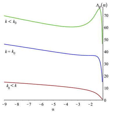
Figure 1: Plot of $\Lambda_{q}\left(\alpha\right)$ as a function of $\alpha$ depicted for $q=1$. The local minimum and the local maximum appear below the critical scale $k_{0}$. For $k=k_{0}$ there is only a stationay point which disappears for $k>k_{0}$.

As depicted in Fig.$\left(\ref{Lambda}\right)$, the couple $\left(k_{0},\bar{\alpha}\right)$ does not represent the solution of the problem, because the point is stationary and not a local minimum. Rather we can interpret the couple $\left(k_{0},\bar{\alpha}\right)$ as a critical value below which a minimum and a maximum appear. In particular, as shown in Fig..$\left(\ref{Lambda}\right)$, for $k<k_{0}$ and $\alpha<\bar{\alpha}$ we have a minimum and for $k<k_{0}$ and $\alpha>\bar{\alpha}$, we have a maximum. In the spirit of the variational procedure only the minimum can be considered as the solution of the problem. Note that the lower the value of $k_{0}$, the higher the value of $\Lambda_{q}\left(\bar{\alpha}\right)$. Note also that the value of $k_{0}$ is transplanckian. From the expression of $\Lambda_{q}\left(\alpha\right)$, this is true when ${\alpha>0}$ or when ${\alpha<-2/3}$, otherwise when ${-2/3<\alpha<0}$, the behavior on $k$ reverses. From the assumption $\left(\ref{c(t)}\right)$, we see that for ${\alpha>0}$, we have $c\left(t\right)\gg c_{0}$ when the scale factor $a\left(t\right)\gg a_{0}$ and this is ruled out by observation. Therefore, the correct range of solutions is when ${\alpha<-2/3}$. Furthermore to have also positive solutions we need ${\alpha<-1}$. The physical reason of why we obtain solutions in the negative range of ${\alpha}$ is that in the early universe one expects to measure strong quantum effects when the scale factor $a\left(t\right)$ is really small. In this framework, this is realized with a speed of light which is really big compared to $c_{0}$. It is interesting to note that for $k>k_{0}$, there is no solution at all and for $k\gg k_{0}$, $\Lambda_{q}\left(\alpha\right)\ll 1$ in Planck’s units and $\alpha\in\left(\bar{\alpha}-\varepsilon,\bar{\alpha}\right)$ with $\varepsilon>0$ arbitrarily small.

IV Conclusions

Motivated by the results obtained in different contexts of distorted gravity and in special way in the HL theoryRemoHL , in this paper we have examined the possibility that the cosmological constant can be considered as an eigenvalue of an appropriate Sturm-Liouville problem of a VSL theory. This interpretation is not new and it has been explored in different contextsGMLM ; GMLM1 ; RemoHL . What is different in this paper is that the WDW equation on a FLRW background in a mini-superspace approach reveals a complete analogy with a Sturm-Liouville problem and the cosmological constant has the natural interpretation of its related eigenvalue. The WDW equation has been examined taking account of the factor order ambiguity. We have probed ordinary gravity without matter fields with different families of trial wave functions and we have found no sign of a cosmological constant induced by quantum fluctuations. Of course we have not exhausted all the possible choices of the trial wave functions. However, the form we have adopted has been chosen using the standard criteria for a variational approach. Therefore, we can conjecture that for a mini-superspace approach without matter fields, a cosmological constant cannot be generated. The introduction of a VSL

$$c\left(t\right)=c_{0}\left(\frac{a\left(t\right)}{a_{0}}\right)^{\alpha}$$ (69)

makes the situation different because of the power law on the scale factor. This modification is also supported by the following alternative definition of the speed of light

$$c\left(E/E_{\mathrm{Pl}}\right)=\frac{dE}{dp}=c_{0}\frac{g_{2}\left(E/E_{\mathrm{Pl}}\right)}{g_{1}\left(E/E_{\mathrm{Pl}}\right)},$$ (70)

which can be easily extracted if one introduces Gravity’s Rainbow into the FLRW metric. In this formulation, the space-time geometry is described by the deformed metric

$$ds^{2}=-\frac{N^{2}\left(t\right)}{g_{1}^{2}\left(E/E_{\mathrm{Pl}}\right)}dt^{2}+\frac{a^{2}\left(t\right)}{g_{2}^{2}\left(E/E_{\mathrm{Pl}}\right)}d\Omega_{3}^{2}~{},$$ (71)

where $g_{1}(E/E_{\mathrm{Pl}})$ and $g_{2}(E/E_{\mathrm{Pl}})$ are functions of energy, which incorporate the deformation of the metric. Concerning the low-energy limit it is required to consider

$$\lim_{E/E_{\mathrm{Pl}}\rightarrow 0}g_{1}\left(E/E_{\mathrm{Pl}}\right)=1\qquad\mathrm{and}\qquad\lim_{E/E_{\mathrm{Pl}}\rightarrow 0}g_{2}\left(E/E_{\mathrm{Pl}}\right)=1,$$ (72)

and thus to recover the usual background $\left(\ref{FRW}\right)$. Hence, $E$ quantifies the energy scale at which quantum gravity effects become apparent. For instance, one of these effects would be that the graviton distorts the background metric as we approach the Planck scale. In a distorted FLRW metric the dispersion relation for a massless graviton is

$$E^{2}g_{1}^{2}\left(\frac{E}{E_{P}}\right)=p^{2}g_{2}^{2}\left(\frac{E}{E_{P}}\right),$$ (73)

leading to $\left(\ref{c(E)}\right)$. Setting for example

$$g_{1}\left(E/E_{\mathrm{Pl}}\right) =1$$

$$g_{2}\left(E/E_{\mathrm{Pl}}\right) =1+\left(\frac{a\left(t\right)}{a_{0}}\right)^{\alpha},$$ (74)

one obtains a different, but equivalent form of the VSL. This formulation has the advantage to avoid technical complications as in Ref.RGES . The choice in $\left(\ref{VSLb}\right)$ appears to be connected also to the following potential

$$a^{4}\left(t\right)\left[\frac{6}{a^{2}\left(t\right)}-\frac{96\pi Gb}{a^{4}\left(t\right)}-\frac{\allowbreak 3456\pi^{2}G^{2}c}{a^{6}\left(t\right)}-2\Lambda\right],$$ (75)

coming from a HL theory without detailed balanced condition. In this kind of potential, one discovers positive eigenvalues depending on the various coupling constants choices. However the potential $\left(\ref{HL}\right)$ appears to be more flexible to produce positive eigenvalues. It is for this reason that the structure of the trial wave function we have used in this paper is more elaborated compared to a simple gaussian function which has bees used in a HL theoryRemoHL . The procedure of finding a minimum for $\Lambda\left(\beta\right)$ of Eq.$\left(\ref{LB}\right)$ has produced a result depending on two other parameters, the power $\alpha$ and the reference scale $k$. A further minimization procedure allows to select one value compatible with the procedure which however does not constitute the final answer, rather it has been interpreted as a critical value below which we have eigenvalues while above which we have none. Note that the appearance of eigenvalues compatible with the procedure is in the transplanckian regime and for negative values of $\alpha$. Negative values of $\alpha$ have been found in Ref.harko , even if the authors discuss the “Creation from Nothing” problem. Note that for Planckian and cisplanckian values of the scale $a_{0}$, the eigenvalue does not appear and for larger scales, like the inflationary one, the whole expression in $\left(\ref{Lq}\right)$ becomes very small for every value of $\alpha<-1$. At this stage of calculation, we do not know if this behavior is simply a failure of the approach or further information can be extracted.

Appendix A Integrals for $\Psi\left(a\right)=\exp\left(-\frac{\beta{a}^{2}}{2}\right)U{\left(\frac{q+1}{4},\frac{q+1}{2},\beta{a}^{2}\right)}$

If the trial wave function assumes the form

$$\Psi\left(a\right)=\exp\left(-\frac{\beta{a}^{2}}{2}\right)U{\left(\frac{q+1}{4},\frac{q+1}{2},\beta{a}^{2}\right),}$$ (76)

then, for practical purposes, it can be transformed into

$$\Psi\left(a\right)={\frac{\left(\beta{a}^{2}\right)^{\left(1-q\right)/4}}{\sqrt{\pi}}K_{\left(q-1\right)/4}{\left(\frac{\beta{a}^{2}}{2}\right)},}$$ (77)

where we have used the identity $\left(\ref{Kummer}\right)$

$$U{\left(a+1/2,2a+1,2x\right)=}\mathrm{\exp}\left(x\right)K_{a}{\left(x\right)/}\left(\sqrt{\pi}\left(2x\right)^{a}\right),$$ (78)

with $a=\left(q-1\right)/4$ and $x=\beta{a}^{2}/2$. Plugging the trial wave function $\left(\ref{BesselK}\right)$ into the kinetic term, one gets

$$\left[-\frac{\partial^{2}}{\partial a^{2}}-\frac{q}{a}\frac{\partial}{\partial a}\right]\Psi\left(a\right)$$

$$=-\beta^{2}a^{2}\exp\left(-\frac{\beta{a}^{2}}{2}\right)U{\left(\frac{q+1}{4},\frac{q+1}{2},\beta{a}^{2}\right).}$$ (79)

If we multiply the expression $\left(\ref{HPsi}\right)$ on the left by $a^{q}\Psi^{\ast}\left(a\right)$ and we integrate over the scale factor, we find

$$\int_{0}^{\infty}daa^{q}\Psi^{\ast}\left(a\right)\left[-\frac{\partial^{2}}{\partial a^{2}}-\frac{q}{a}\frac{\partial}{\partial a}\right]\Psi\left(a\right)=-\beta^{2}\int_{0}^{\infty}daa^{q+2}\exp\left(-\beta{a}^{2}\right)U^{2}{\left(\frac{q+1}{4},\frac{q+1}{2},\beta{a}^{2}\right)}$$

$$=-\,\frac{\beta^{\frac{5-q}{2}}}{\pi}\int_{0}^{\infty}daa^{3}K_{\left(q-1\right)/4}^{2}{\left(\frac{\beta{a}^{2}}{2}\right)}$$

$${\underset{\sqrt{\beta/2}a=\sqrt{x}}{=}-}\frac{{2}}{\pi}\beta^{\frac{1-q}{2}}\int_{0}^{\infty}dxxK_{\left(q-1\right)/4}^{2}{\left(x\right)}=-\frac{\beta^{\frac{1-q}{2}}}{\pi}\Gamma\left(\frac{3+q}{4}\right)\Gamma\left(\frac{5-q}{4}\right),$$ (80)

where we have used the following relationshipPBM

$$\int_{0}^{\infty}dxx^{\alpha-1}K_{\mu}{\left(cx\right)}K_{\nu}{\left(cx\right)}$$

$$=\frac{2^{\alpha-3}}{c^{\alpha}\Gamma\left(\alpha\right)}\Gamma\left(\frac{\alpha+\mu+\nu}{2}\right)\Gamma\left(\frac{\alpha+\mu-\nu}{2}\right)\Gamma\left(\frac{\alpha+\nu-\mu}{2}\right)\Gamma\left(\frac{\alpha-\mu-\nu}{2}\right)$$

$$\operatorname{Re}c>0;\operatorname{Re}\alpha>\left|\operatorname{Re}\nu\right|+\left|\operatorname{Re}\mu\right|.$$ (81)

and where $\Gamma\left(x\right)$ is the gamma function. The contribution coming from the potential term without the VSL distortion is composed by

$$\int_{0}^{\infty}daa^{q}\Psi^{\ast}\left(a\right)a^{2}\Psi\left(a\right)=\int_{0}^{\infty}daa^{q+2}\exp\left(-\beta{a}^{2}\right)U^{2}{\left(\frac{q+1}{4},\frac{q+1}{2},\beta{a}^{2}\right)}$$

$$=\frac{\beta^{\frac{1-q}{2}}}{\pi}\int_{0}^{\infty}daa^{3}K_{\left(q-1\right)/4}^{2}{\left(\frac{\beta{a}^{2}}{2}\right)}$$

$${\underset{\sqrt{\beta/2}a=\sqrt{x}}{=}2}\frac{\beta^{-\frac{3+q}{2}}}{\pi}\int_{0}^{\infty}dxxK_{\left(q-1\right)/4}^{2}{\left(x\right)}=\frac{1}{\pi\beta^{\frac{3+q}{2}}}\Gamma\left(\frac{3+q}{4}\right)\Gamma\left(\frac{5-q}{4}\right)$$ (82)

and

$$\int_{0}^{\infty}daa^{q}\Psi^{\ast}\left(a\right)a^{4}\Psi\left(a\right)=\int_{0}^{\infty}daa^{q+4}\exp\left(-\beta{a}^{2}\right)U^{2}{\left(\frac{q+1}{4},\frac{q+1}{2},\beta{a}^{2}\right)}$$

$$=\frac{\beta^{\frac{1-q}{2}}}{\pi}\int_{0}^{\infty}daa^{5}K_{\left(q-1\right)/4}^{2}{\left(\frac{\beta{a}^{2}}{2}\right)}$$

$${\underset{\sqrt{\beta/2}a=\sqrt{x}}{=}4}\frac{\beta^{-\frac{5+q}{2}}}{\pi}\int_{0}^{\infty}dxx^{2}K_{\left(q-1\right)/4}^{2}{\left(x\right)=\frac{1}{2\beta^{\frac{5+q}{2}}}\Gamma\left(\frac{5+q}{4}\right)\Gamma\left(\frac{7-q}{4}\right)}.$$ (83)

The contribution coming from the potential term with the VSL distortion is composed by

$$\int_{0}^{\infty}daa^{q}\Psi^{\ast}\left(a\right)a^{2+6\alpha}\Psi\left(a\right)=\int_{0}^{\infty}daa^{q+2+6\alpha}\exp\left(-\beta{a}^{2}\right)U^{2}{\left(\frac{q+1}{4},\frac{q+1}{2},\beta{a}^{2}\right)}$$

$$=\frac{\beta^{\frac{1-q}{2}}}{\pi}\int_{0}^{\infty}daa^{3+6\alpha}K_{\left(q-1\right)/4}^{2}{\left(\frac{\beta{a}^{2}}{2}\right)\underset{\sqrt{\beta/2}a=\sqrt{x}}{=}}\frac{{2}^{1+3\alpha}}{\pi\beta^{2+3\alpha+\frac{q-1}{2}}}\int_{0}^{\infty}dxx^{1+3\alpha}K_{\left(q-1\right)/4}^{2}{\left(x\right)}$$

$$=\frac{{2}^{6\alpha}}{\pi\beta^{\frac{3+q}{2}+3\alpha}\Gamma\left(2+3\alpha\right)}\Gamma\left(\frac{3+6\alpha+q}{4}\right)\Gamma^{2}\left(\frac{2+3\alpha}{2}\right)\Gamma\left(\frac{5+6\alpha-q}{4}\right)$$ (84)

and

$$\int_{0}^{\infty}daa^{q}\Psi^{\ast}\left(a\right)a^{4+6\alpha}\Psi\left(a\right)=\int_{0}^{\infty}daa^{q+4+6\alpha}\exp\left(-\beta{a}^{2}\right)U^{2}{\left(\frac{q+1}{4},\frac{q+1}{2},\beta{a}^{2}\right)}$$

$$=\frac{\beta^{\frac{1-q}{2}}}{\pi}\int_{0}^{\infty}daa^{5+6\alpha}K_{\left(q-1\right)/4}^{2}{\left(\frac{\beta{a}^{2}}{2}\right)\underset{\sqrt{\beta/2}a=\sqrt{x}}{=}}\frac{2^{2+3\alpha}}{\pi\beta^{3+3\alpha+\frac{q-1}{2}}}\int_{0}^{\infty}dxx^{2+3\alpha}K_{\left(q-1\right)/4}^{2}{\left(x\right)}$$

$${=\frac{2^{2+6\alpha}}{\pi\beta^{\frac{5+q}{2}+3\alpha}\Gamma\left(3+3\alpha\right)}\Gamma\left(\frac{5+6\alpha+q}{4}\right)\Gamma}^{2}{\left(\frac{3+3\alpha}{2}\right)\Gamma\left(\frac{7+6\alpha-q}{4}\right)}.$$ (85)

Appendix B Integrals for $\Psi\left(a\right)={a}^{-\frac{q+1}{2}}\left(\beta{a}\right)^{\frac{\rho}{2}}\exp\left(-\frac{\beta{a}^{\lambda}}{2}\right)$

If the trial wave function assumes the form

$$\Psi\left(a\right)={a}^{-\frac{q+1}{2}}\left(\beta{a}\right)^{\frac{\rho}{2}}\exp\left(-\frac{\beta{a}^{\lambda}}{2}\right){,}$$ (86)

when we plug the trial wave function $\left(\ref{BesselK}\right)$ into the kinetic term, one gets

$$\left[-\frac{\partial^{2}}{\partial a^{2}}-\frac{q}{a}\frac{\partial}{\partial a}\right]\Psi\left(a\right)=\frac{1}{4}\,\exp\left(-\frac{\beta{a}^{\lambda}}{2}\right)\beta^{\frac{\rho}{2}}{a}^{\frac{\rho-5-q}{2}}\left[\left({q}^{2}-{\rho}^{2}+4\rho-2q-3\right)\right.$$

$$=\left.2{\beta a}^{\lambda}\left({\lambda}^{2}+\rho\,\lambda-2\lambda\right)-{a}^{2\,\lambda}{\beta}^{2}{\lambda}^{2}\right]{.}$$ (87)

If we multiply the expression $\left(\ref{HPsi}\right)$ on the left by $a^{q}\Psi^{\ast}\left(a\right)$ and we integrate over the scale factor, we find

$$\int_{0}^{\infty}daa^{q}\Psi^{\ast}\left(a\right)\left[-\frac{\partial^{2}}{\partial a^{2}}-\frac{q}{a}\frac{\partial}{\partial a}\right]\Psi\left(a\right)={\frac{\lambda\rho+{q}^{2}-2\lambda-2\,q+1}{4\lambda}\Gamma\left({\frac{-2+\rho}{\lambda}}\right){\beta}^{{\frac{\lambda\rho-\rho+2}{\lambda}}}},$$ (88)

where $\Gamma\left(x\right)$ is the gamma function. The contribution coming from the potential term with the VSL distortion is composed by

$$\int_{0}^{\infty}daa^{q}\Psi^{\ast}\left(a\right)a^{2+6\alpha}\Psi\left(a\right)=\int_{0}^{\infty}daa^{1+6\alpha+\rho}\beta^{\rho}\exp\left(-\beta{a}^{\lambda}\right)$$

$$={\frac{1}{\lambda}{\beta}^{{\frac{\lambda\rho-6\alpha-\rho-2}{\lambda}}}\Gamma\left({\frac{2+6\alpha+\rho}{\lambda}}\right)}$$ (89)

and

$$\int_{0}^{\infty}daa^{q}\Psi^{\ast}\left(a\right)a^{4+6\alpha}\Psi\left(a\right)=\int_{0}^{\infty}daa^{3+6\alpha+\rho}\beta^{\rho}\exp\left(-\beta{a}^{\lambda}\right)$$

$$={\frac{1}{\lambda}{\beta}^{{\frac{\lambda\rho-6\alpha-\rho-4}{\lambda}}}\Gamma\left({\frac{4+6\alpha+\rho}{\lambda}}\right)}$$ (90)

References

- (1) B. S. DeWitt, Phys. Rev. 160, 1113 (1967).
- (2) R. Arnowitt, S. Deser, and C. W. Misner, in Gravitation: An Introduction to Current Research, edited by L. Witten (John Wiley & Sons, Inc., New York, 1962); B. S. DeWitt, Phys. Rev. 160, 1113 (1967). arXiv:gr-qc/0405109.
- (3) S. Capozziello and M.De Laurentis, Phys. Rept. 509, 167 (2011); arXiv:1108.6266 [gr-qc]. S. Nojiri and S. D. Odintsov, Phys. Rept. 505, 59 (2011); arXiv:1011.0544 [gr-qc]. T. P. Sotiriou and V. Faraoni, Rev. Mod. Phys. 82, 451 (2010); arXiv:0805.1726 [gr-qc].
- (4) P. Hǒrava, JHEP, 0903, 020 (2009). ArXiv: 0812.4287 [hep-th]; P. Hǒrava, Phys. Rev. Lett. 102, 161301 (2009) ArXiv: 0902.3657 [hep-th].
- (5) E.M. Lifshitz, Zh. Eksp. Toer. Fiz. 11, 255; 269 (1941).
- (6) J. Magueijo and L. Smolin, Class. Quant. Grav. 21, 1725 (2004) [arXiv:gr-qc/0305055].
- (7) S. Alexander and J. Magueijo, Noncommutative geometry as a realization of varying speed of light cosmology in Proceedings of the XIIIrd Rencontres de Blois, pp281, 2004 [arXiv:hep-th/0104093].
- (8) R. Garattini and G. Mandanici, Phys. Rev. D 83 084021 (2011); [arXiv:1102.3803 [gr-qc]]. R. Garattini, JCAP 1306 (2013) 017; arXiv:1210.7760 [gr-qc]. R. Garattini and B. Majumder, Nucl. Phys. B 884 125, (2014) [arXiv:1311.1747 [gr-qc]].
- (9) R. Garattini, Phys.Lett. B 685 329 (2010); [arXiv:0902.3927 [gr-qc]]. R. Garattini and F. S.N. Lobo, Phys. Rev. D 85 024043 (2012); [arXiv:1111.5729 [gr-qc]]. R. Garattini and G. Mandanici, Phys. Rev. D 85 023507 (2012); [arXiv:1109.6563 [gr-qc]]. R. Garattini and B. Majumder, Nucl. Phys. B 883 598, (2014); [arXiv:1305.3390 [gr-qc]. R. Garattini and F. S. N. Lobo, Eur. Phys. J. C 74 2884, (2014); [arXiv:1303.5566 [gr-qc]].
- (10) R. Garattini, Phys. Rev. D 86 123507 (2012); [arXiv:0912.0136 [gr-qc]].
- (11) O. Bertolami and C. A. D. Zarro, Phys. Rev. D 84 044042, (2011); [arXiv:1106.0126 [hep-th]]
- (12) A. V. Astashenok, E. Elizalde and A. V. Yurov, Astrophys. Space Sci. 349 25 (2014);[arXiv:1212.4268 [astro-ph.CO]].
- (13) R. Garattini and E. N. Saridakis, Gravity’s Rainbow: a bridge towards Horava-Lifshitz gravity, [arXiv:1411.7257 [gr-qc]].
- (14) T. Harko and M. K. Mak, Class. Quantum Grav. 16, 2741 (1999).
- (15) J. W. Moffat, Int. J. Mod. Phys. D 2 351, (1993).
- (16) A. Albrecht and J. Magueijo, Phys. Rev. D 59, 043516 (1999).
- (17) J. D. Barrow, Phys. Rev. D 59,043515 (1999).
- (18) J. D. Barrow and J. Magueijo, Phys. Lett. B 443, 104 (1999).
- (19) J. D. Barrow and J. Magueijo, Phys. Lett. B 447,246 (1999).
- (20) E. W. Kolb and M. S. Turner, The Early Universe (Wiley, New York, 1990).
- (21) A.H. Guth, Phys. Rev. D 23, 347 (1981).
- (22) A. Linde, Phys. Lett. B 108, 389 (1982).
- (23) A. Albrecht and P. Steinhardt, Phys. Rev. Lett. 48, 1220 (1982).
- (24) G. Veneziano, Phys. Lett. B 406, 297 (1997).
- (25) G.F.R. Ellis, Gen. Rel. Grav., 39, 511 (2007).
- (26) J. Magueijo, Phys. Rev. D 62, 103521 (2000).
- (27) J. Magueijo, J. W. Moffat, Gen.Rel.Grav. 40, 1797 (2008).
- (28) A. Vilenkin, Phys. Rev. D 37 (1988) 888.
- (29) J. B. Hartle and S. W. Hawking, Phys. Rev. D 28 (1983) 2960; S. W. Hawking, Nucl. Phys. B 239 (1984) 257.
- (30) T. Harko, H. Q. Lu, M. k. Mak and K. S. Cheng, Europhys. Lett. 49, 814 (2000).
- (31) F. Shojai, S. Molladavoudi, Gen. Relativ. Gravit. 39, 795 (2007).
- (32) . J. W. Moffat, Published in “Janke, W. (ed.) et al.: Fluctuating paths and fields” 741-757; preprint astro-ph/9811390 (1998). ;
- (33) T. Harko, H. Q. Lu, M. K. Mak and K. S. Cheng, Europhys. Lett., 49 (6), pp. 814–820 (2000). A.V. Yurov and V.A. Yurov, “The semiclassical tunneling probability in quantum cosmologies with varying speed of light”, arXiv:hep-th/0410231.
- (34) J. Magueijo and L. Smolin, Phys. Rev. D 67 (2003) 044017 [arXiv:gr-qc/0207085].
- (35) D. L. Wiltshire, An introduction to quantum cosmology. [gr-qc/0101003]. D. L. Wiltshire, Gen.Rel.Grav. 32, 515 (2000); [arXiv: gr-qc/9905090]. N. Kontoleon and D.L. Wiltshire, Phys. Rev. D 59, 063513 (1999); [arXiv: gr-qc/9807075].
- (36) S. Watson, M. J. Perry, G. L. Kane and F. C. Adams, JCAP 0711 017 (2007); [arXiv: hep-th/0610054].
- (37) A. P. Prudnikov, Yu. A. Brychkov and O.I. Marichev, Integrals and Series,Vol. 2: More Special Functions, edited by Gordon and Breach Science Publishers, Second Printing 1998.