The Relationship Between the Dust and Gas-Phase CO Across the California Molecular Cloud
Abstract
We present results of an extinction–CO line survey of the southeastern part of the California Molecular Cloud (CMC). Deep, wide-field, near-infrared images were used to construct a sensitive, relatively high resolution ( 0.5 arc min) (NICEST) extinction map of the region. The same region was also surveyed in the 12CO(2-1), 13CO(2-1), C18O(2-1) emission lines at the same angular resolution. These data were used to investigate the relation between the molecular gas, traced by CO emission lines, and the dust column density, traced by extinction, on spatial scales of 0.04 pc across the cloud. We found strong spatial variations in the abundances of 13CO and C18O that were correlated with variations in gas temperature, consistent with temperature dependent CO depletion/desorption on dust grains. The 13CO to C18O abundance ratio was found to increase with decreasing extinction, suggesting selective photodissociation of C18O by the ambient UV radiation field. The effect is particularly pronounced in the vicinity of an embedded cluster where the UV radiation appears to have penetrated deeply (i.e., AV 15 mag) into the cloud. We derived the cloud averaged X-factor to be XCO 2.53 1020 , a value somewhat higher than the Milky Way average. On sub-parsec scales we find there is no single empirical value of the 12CO X-factor that can characterize the molecular gas in cold (Tk 15 K) cloud regions, with XCO A for AV 3 magnitudes. However in regions containing relatively hot (Tex 25 K) molecular gas we find a clear correlation between W(12CO) and AV over a large (3 AV 25 mag) range of extinction. This results in a constant XCO 1.5 1020 for the hot gas, a lower value than either the average for the CMC or the Milky Way. Overall we find an (inverse) correlation between XCO and Tex in the cloud with XCO Tex-0.7. This correlation suggests that the global X-factor of a Giant Molecular Cloud (GMC) may depend on the relative amounts of hot gas contained within the cloud.
Subject headings:
stars: formation; ISM: clouds; (ISM:) dust, extinction; ISM: abundances1. Introduction
The relationship between the dust and gas in a molecular cloud is crucial in understanding the cloud properties and the star formation activities therein. Dust provides the most reliable and useful tracer of the total gas column density (e.g., Bohlin et al., 1978; Rachford et al., 2009; Goodman et al., 2009), while molecules like 13CO and C18O are more useful as tracers of the local physical and chemical conditions (e.g., gas temperatures and velocities, CO column densities, etc.) A comparison between them allows us to probe the variation of molecular gas abundances, i.e., [13CO] and [C18O] ([molecule] N(molecule)/N(H) where N is column density), caused by such factors as photodissociation and chemical depletion/desorption in cold/warm environments. This helps to reveal the physical and chemical properties of the molecular cloud, which enables us to better understand the initial conditions of star formation and its potential dependence on such factors as cloud chemistry and structure. Such variations have been noted in previous observations of a variety of GMCs, including Perseus (Pineda et al., 2008), Taurus (Pineda et al., 2010), and Orion (Ripple et al., 2013), made at relatively high spatial resolutions (0.2 - 0.4 pc). Here we report the results of a combined CO-dust extinction study of the California molecular cloud (CMC, Lada, Lombardi, & Alves, 2009) at even higher spatial resolution ( 0.04 pc) in order to investigate in more detail the relation between CO gas and dust in this interesting nearby GMC.
The CMC is a useful laboratory for such studies. In particular, it contains a massive filamentary structure in its southeast region that consists of both cold molecular gas with little star formation activity and hot molecular gas associated with an active star forming region containing the massive star LkH 101 and its accompanying embedded cluster. This provides a physical environment with large temperature and density variations that are interesting to explore. Indeed, as reported in Lada, Lombardi, & Alves (2009), the CMC overall shows an order of magnitude lower star formation rate (SFR) than the Orion molecular cloud, even though these equally distant GMCs have similar mass, size, and morphology. Recently, Li et al. (2014) also found the 13CO clumps in the CMC to be characterized by similar kinematic states as those in Orion. Lada, Lombardi, & Alves (2009) proposed that the difference in SFRs between the two clouds was a result of a difference in cloud structure, specifically the amount of dense gas in each cloud. Moreover, this close connection between dense gas mass and the SFR appears to be a general physical property of galactic GMCs (Lada et al., 2010). It would be of interest to compare other properties of the CMC with similar ones in the Orion cloud to look for additional factors, such as cloud chemistry for example, that could contribute to the difference in the SFR between the two clouds.
A combined CO-extinction study can also be used to investigate the CO X-factor (XCO N(H2)/WCO(1-0), where W is integrated intensity) which is widely used to derive molecular cloud masses from the CO(1-0) line flux, especially in external galaxies (see e.g. Sandstrom et al., 2013; Bolatto et al., 2013). Despite being very optically thick, this CO rotational transition is still thought to be a good tracer for the total molecular gas mass, due to the effect of photon transport in gas with large velocity gradients. However, variations of physical conditions can have an effect on the X-factor and, in many instances, render its application rather uncertain. Apparently, there is no universally valid X-factor (see recent review from Bolatto et al., 2013). Consequently, investigating the dependence of the X-factor on differing physical conditions is clearly of great interest in establishing practical guidelines for its application. Combined CO-extinction studies of nearby clouds can therefore provide potentially important insights into this issue.
In this paper, we present observational results of molecular lines 12CO(2-1), 13CO(2-1), and C18O(2-1). The total gas mass (or N) is traced by extinction derived from NIR observations, independent from the molecular lines. The area covered in our observation is mainly dense gas with AV 3 mag. With the NICEST technique (Lombardi, 2009), we are able to trace extinction up to AV 33 mag, which is much deeper than achieved in a similar study of Orion by Ripple et al. (2013) who used the NICER technique (Lombardi & Alves, 2001) to trace extinction depths up to AV 15 mag. We also observed the optically thinner C18O(2-1) line, which provides insights into CO chemistry (e.g., Lada et al., 1994; Shimajiri et al., 2014) that cannot be readily derived using only 12CO and 13CO observations.
2. Observations and Data Reduction
2.1. Near-Infrared Wide-Field Mapping Survey
2.1.1 Telescope and Observations
| Field ID | Date Obs. | Center Coords. | Filter | Seeing | LF PeakaaExpresses turnover point of observed magnitude distribution | |
|---|---|---|---|---|---|---|
| J2000 | [] | [mag] | ||||
| CALAR ALTO 3.5 m OMEGA 2000 OBSERVATIONS | ||||||
| CN-01 | 2009-12-24 | 04:30:58.81 | +34:51:57.5 | 1.49 | 19.00 | |
| CN-01 | 2009-12-24 | 04:30:58.81 | +34:51:57.5 | 1.52 | 19.75 | |
| CN-01 | 2009-12-24 | 04:30:58.81 | +34:51:57.5 | 1.39 | 19.25 | |
| CN-02 | 2009-12-08 | 04:30:38.55 | +35:04:20.4 | 1.36 | 19.50 | |
| CN-02 | 2009-10-09 | 04:30:38.55 | +35:04:20.4 | 1.59 | 20.75 | |
| CN-02 | 2009-10-09 | 04:30:38.55 | +35:04:20.4 | 1.47 | 19.75 | |
| CN-03 | 2012-12-23 | 04:30:07.84 | +35:16:06.6 | 1.11 | 22.25 | |
| CN-03 | 2012-12-23 | 04:30:07.84 | +35:16:06.6 | 1.06 | 20.25 | |
| CN-03 | 2012-12-23 | 04:30:07.84 | +35:16:06.6 | 1.12 | 19.25 | |
| CN-04 | 2009-10-07 | 04:30:44.04 | +35:27:49.5 | 1.05 | 21.25 | |
| CN-04 | 2009-10-07 | 04:30:44.04 | +35:27:49.5 | 0.96 | 19.50 | |
| CN-04 | 2009-10-09 | 04:30:44.04 | +35:27:49.5 | 1.05 | 21.50 | |
| CN-05 | 2009-10-07 | 04:30:44.04 | +35:41:24.1 | 0.91 | 21.25 | |
| CN-05 | 2009-10-07 | 04:30:44.04 | +35:41:24.1 | 0.93 | 22.00 | |
| CN-05 | 2009-10-06 | 04:30:44.04 | +35:41:24.1 | 1.17 | 19.75 | |
| CN-06 | 2009-10-06 | 04:30:44.73 | +35:54:54.8 | 1.29 | 22.00 | |
| CN-06 | 2009-10-06 | 04:30:44.73 | +35:54:54.8 | 1.26 | 21.00 | |
| CN-06 | 2009-10-06 | 04:30:44.73 | +35:54:54.8 | 1.30 | 20.00 | |
| CN-07 | 2010-01-02 | 04:29:08.58 | +36:29:18.7 | 1.07 | 20.75 | |
| CN-07 | 2010-01-02 | 04:29:08.58 | +36:29:18.7 | 1.13 | 19.00 | |
| CN-07 | 2010-01-02 | 04:29:08.58 | +36:29:18.7 | 1.18 | 18.75 | |
| CN-08 | 2010-01-03 | 04:28:16.37 | +36:29:58.4 | 1.37 | 20.25 | |
| CN-08 | 2010-01-03 | 04:28:16.37 | +36:29:58.4 | 1.35 | 20.00 | |
| CN-08 | 2010-01-03 | 04:28:16.37 | +36:29:58.4 | 1.02 | 19.25 | |
Near-IR observations for this study were obtained at the 3.5 m telescope of the Centro Astronómico Hispano Alemán observatory (hereafter CAHA) at Calar Alto in Almería, Spain. Our observations were made with the OMEGA 2000 camera, which has a field of view of 15. In this paper we report observations for eight fields that cover the L1482 region. These fields are part of a more comprehensive survey of the CMC with a total of 24 fields. Fields CN01 to CN08 (Table 1) were observed in the three main near-IR broadbands, , and , between October 2009 and January 2010, with acceptable weather and seeing, except for one field, CN03, which was repeated on December, 2012. All observations consisted of 20 exposures of 60 seconds, coadded as 1200 second exposure mosaics. The fields observed with the CAHA 3.5 m telescope were selected to cover the main filament or “spine” of L1482, including the region of the LkH 101 cluster. The pixel scale of OMEGA 2000 at the 3.5 m telescope is 0.45 , with excellent uniformity and negligible geometric distortion across the FOV.
A list of all fields observed and considered for final analysis can be consulted in table 1. The table lists the field identification, the center of field positions, observation date, filter, an estimate of the seeing based on the average FWHM of the stars detected in each field, and the peak values for the brightness distributions, which are a good measurement of the sensitivity limits achieved. Below, we describe the observations and the data reduction process, including the construction of the photometric catalogs used to make our dust extinction map.
2.1.2 Near-Infrared Data Reduction and Calibration
The near-IR image data from OMEGA 2000 was reduced with pipelines that made use of standard IRAF procedures complemented with stand alone routines. These pipelines are based on the FLAMINGOS near-IR reduction, photometry and astrometry pipelines (Román-Zúñiga, 2006; Levine, 2006). The data process is essentially identical to the one described in Román-Zúñiga et al. (2010) and we refer the reader to that paper for details.
Both photometry and astrometry of OMEGA 2000 data products were calibrated relative to Two-Micron All Sky Survey (2MASS) lists obtained from the All-Sky Point Source Catalog (PSC). The final photometry catalogs were merged with a combination of TOPCAT-STIL (Taylor, 2005) and IDL routines. In the case of adjacent fields, overlapping areas were treated with a routine designed to handle duplicate detections in such a way that we list preferentially a higher quality observation (e.g. a smaller photometric uncertainty) over a lower quality one.
The 2MASS data were also used to replace observations for saturated stars in all our frames. We used, in all cases, lists retrieved from the 2MASS All-Sky Point Source Catalog (PSC) at the Infrared Processing and Analysis Center (IPAC). The final photometry catalogs, containing either J, H, and Ks, or H and Ks photometry were merged with a combination of TOPCAT-STIL (Taylor, 2005) and self-made IDL routines.
2.2. The CO Molecular-Line Survey
2.2.1 Telescope and Observations
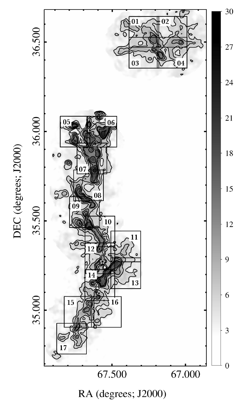
A series of observations were carried out with the Heinrich Hertz Sub-millimeter Telescope (SMT) on Mount Graham, Arizona, from November 2011 to April 2012. The SMT is located at an elevation of 3200 meters. The receiver has prototype ALMA Band 6 sideband separating mixers with two orthogonal polarizations. Typical single sideband system temperatures during the observing were around 200 K. The molecular lines 12CO(2-1) (230.538 GHz), 13CO(2-1) (220.399 GHz), and C18O(2-1) (219.560 GHz) were observed over a selection of 17 square regions (hereafter “tiles”) along the south-eastern dense ridge of the CMC, roughly at RA=, DEC= (see Figure 1, also figure 1 of Lada, Lombardi, & Alves, 2009). These tiles have AV 3 mag, and cover the higher extinction regions of the cloud as well as the LkH 101 cluster (roughly centered in tile 12).
In each tile, we performed the observations using the “on-the-fly (OTF)” mode. The scanning rate was per second along the direction of Right Ascension (RA), with each row being separated by in Declination (DEC). Each sampling point has a 0.4-second integration, corresponding to 4 spatial sampling in RA with a beam size around , therefore the source is fully sampled. The total integration time for each tile is roughly 1 hour. We utilized dual side band mode and had two distinct sets of observations: Obs1: 13CO(2-1) in lower side-band (LSB) and 12CO(2-1) in upper side-band (USB); Obs2: C18O(2-1) in LSB and 12CO(2-1) in USB. In each set, two orthogonal linear polarizations were observed simultaneously. The total bandwidth we cover with the spectrometer is 128 channels of 0.25 MHz each or 32 MHz total, for each line (12CO, 13CO, and C18O). The channel resolution is 0.25 MHz, set by the filter widths, and this corresponds to about 0.34 velocity resolution, depending on the line rest frequencies via the doppler formula. We checked the pointing on the compact nearby CO source CRL618 (RA=, DEC=) at the beginning of every tile. Five-second integrations were performed on each point of a 5-point cross pattern centered on that source. The pointing error was typically 5. To calibrate the intensity, we observed the strong CO source W3OH (RA=, DEC=) between every two tiles.
2.2.2 Millimeter-wave Data Reduction
All data were first processed through the CLASS software package. We fitted linear baselines and subtracted them from the data. The data image cubes were ported into MIRIAD software format (Sault et al., 1995) for further analysis and display. OTF data were interpolated onto regular grids with grid spacing of 10 before being stored into the MIRIAD data set. Next the data were calibrated using W3OH. A scale factor is derived through the observation toward W3OH between every two tiles. The factor is used to scale the antenna temperature to the main-beam brightness temperature Tmb (see Bieging et al., 2010, for details). For each molecular transition, the two polarizations were averaged to increase the SNR. Finally all 17 tiles were combined together to form a single map (weighted by their RMS noise at the small overlapped area). The original data cube, with 0.34 km s-1 velocity channels (set by the 0.25 MHz filter bandwidth) were re-sampled onto a 0.15 km s-1 spacing, by 3rd-order polynomial interpolation. This re-sampling puts all of the CO isotopologues on exactly the same velocity grid, so we can make ratio maps, for example. We convolved all maps with Gaussian kernels (FWHM = 18.1 for 12CO map, FWHM = 13.6 for 13CO and C18O maps) to have a final map resolution (FWHM) of 38 with a grid spacing of 19 in order to match the resolution of and facilitate direct comparison with our dust extinction maps.
We calculated the RMS noise for all emission-free channels in each map to be about 0.1 K for all three lines. We compared the integrated intensity maps of the two sets of 12CO maps by subtracting one from the other. We found a small spatial difference (typically 10 between each pair of corresponding tiles), and we shifted and re-gridded Obs1 12CO and 13CO maps to Obs2. We averaged the two sets of 12CO maps weighted by their RMS noise to lower the noise in the averaged 12CO map to 0.07 K (RMS).
3. Results and Analysis
3.1. The NICEST Dust Extinction Map
Figure 1 shows the deep dust extinction map of the southeast portion of the CMC derived from our observations. For this map Calar Alto data were supplemented with data from 2MASS in some outer portions of the surveyed area where Calar Alto data were not available. Also shown are the boundaries of the 17 tiles of the multi-line CO mapping survey. The extinction map was constructed with the optimized version of the Near Infrared Color Excess Revised (NICER) technique, known as NICEST (Lombardi & Alves, 2001; Lombardi, 2009). The NICER/NICEST technique allows us to measure dust extinction from the infrared excess in the colors of background stars caused by dust absorption. The excess is derived by assuming as intrinsic colors, the colors of stars detected in a nearby off-cloud control field with negligible extinction (see Table 1). For the measurements of extinction, we avoid the use of sources with intrinsic color excess, such as candidate young stellar objects and dusty galaxies. NICEST is essentially identical to NICER, except that the AV estimator is modified to account for small-scale inhomogeneities, due to a bias introduced by the decrease in the number of observable stars as extinction increases toward the denser areas of a molecular cloud. The bias is removed by modifying the estimator with an additional term that accounts for the expected decrement.
Extinction measurements for individual sources are smoothed with Gaussian filter with a FWHM of 38, and the maps are constructed with 19 spatial sampling. At each (line-of-sight) position in the map, each star falling within the beam is given a weight calculated from a Gaussian function, and the inverse of the variance squared, which is in turn also used for the bias-correction factor. A preliminary value of AV at the map position is calculated as the weighted median of all possible values within the beam. Then, we estimate the mean absolute deviation (m.a.d.) of these values to remove large deviates using m.a.d.-clipping. The remaining values are used by the NICEST estimator to calculate the final AV at the corresponding position.
In the case of pixel positions where only 2MASS sources are available, the number of sources per beam is significantly smaller, and there are cases where there are not enough stars to estimate AV; in those cases, our code increases the size of the beam by a factor of 2 over the nominal value. The nominal 38 FWHM of our maps represents an increase of resolution by a factor of 2.1 compared to the earlier study of Lada, Lombardi, & Alves (2009). This resolution is comparable to the beam size of the CO maps. The resulting noise of extinction map is 0.05 mag for AV 10 mag and 0.1 mag for AV 10 mag.
3.2. CO Spectra and Integrated Intensity Maps
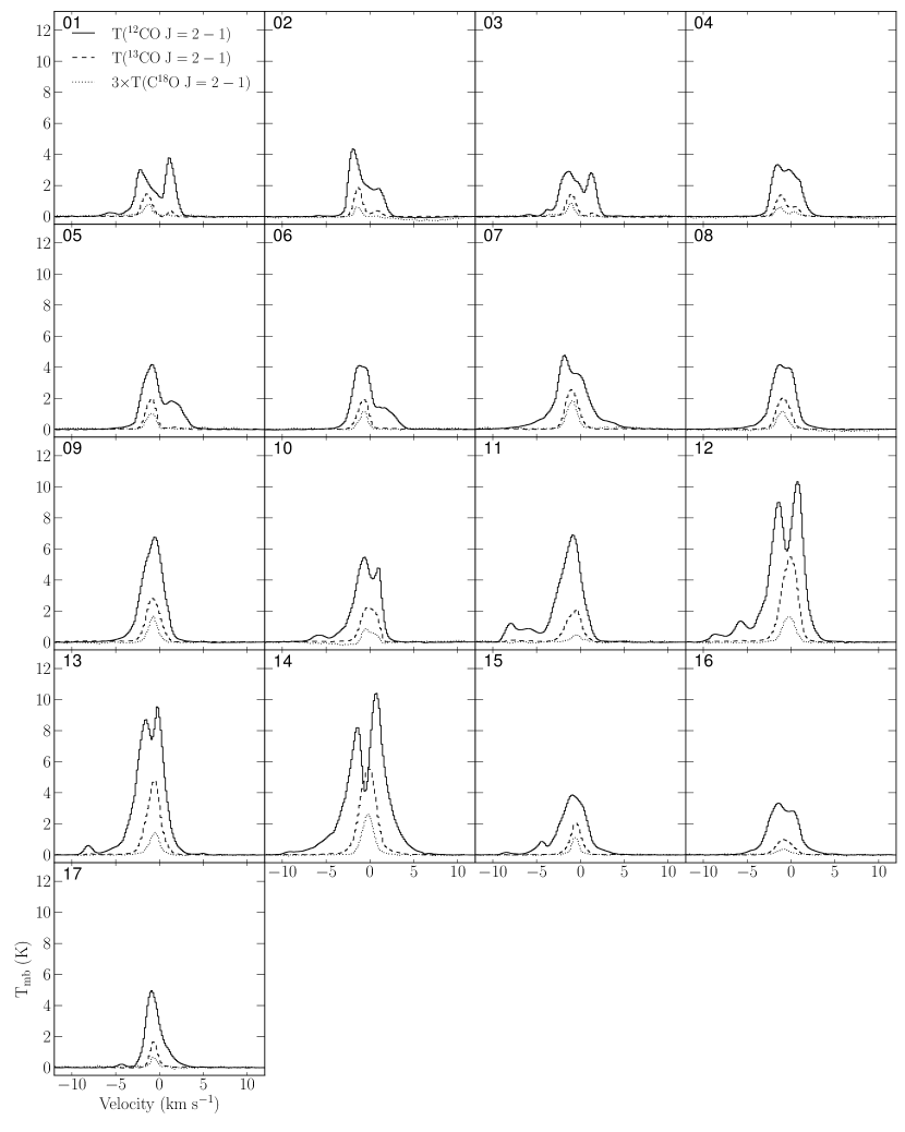
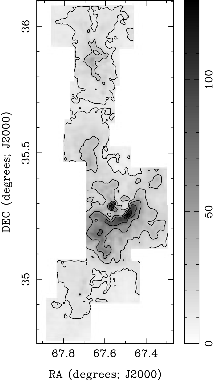
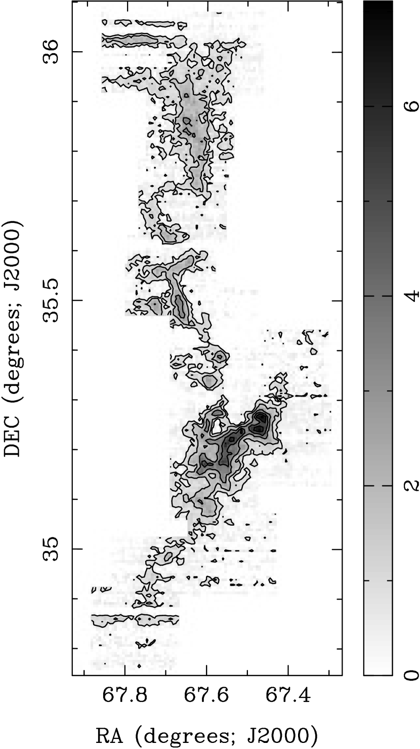
In order to provide an overview of the observations and the general quality of the data we first show in Figure 2 the averaged CO spectra derived for each of the tiles of our mapping grid. On this coarse scale (1.3 1.3 pc) the 12CO profiles exhibit evidence for both self-absorption and multi-component structure. The presence of self-absorption indicates that the 12CO emission is quite optically thick. The profiles of the rarer isotopes appear to be less complex, mostly characterized by simple Gaussian-like shapes. Maps of the emission from 12CO(2-1), 13CO(2-1), C18O(2-1) integrated over velocity ranges, 12 to 10 km s-1, 10 to 6 km s-1, 4 to 3 km s-1, respectively, are shown in Figure 3 as grey scale maps with contours overlaid for clarity. The maps display some common morphological features. The strongest emission occurs in the mid-southern area (tiles 11-14, ) and is in close proximity to the LkH 101 cluster (which lies within tiles 10-12, ). On close inspection of the maps, a sharp drop off in CO emission is observed along a warm filamentary structure southwest of the cluster. This sharp drop in CO emission together with the enhanced CO emission within the warm filament likely indicates a physical interaction between the cluster stars and the filamentary ridge structure. A similar structure with an accompanying drop off is also present in the extinction map of Figure 1. Here we can see that the warm filamentary structure is a small section of the more extended high extinction ridge that forms the backbone of the cloud in this region and which is the subject of this survey. In these more extended regions away from the cluster, the CO emission is comparatively quiescent.
(a) (b) (c)

The RMS noise for the integrated intensity maps (in K km s-1) was first estimated using
| (1) |
where (in K) is the RMS noise per channel derived for emission-free velocities, is the velocity width over which the integrated intensity is calculated. Nchannel here is the number of real independent channels or filters (of bandwidth 0.25 MHz, 0.34 km s-1) within . The estimated for 12CO(2-1), 13CO(2-1), C18O(2-1) integrated intensity maps are 0.16, 0.22, 0.16 , respectively. We also calculated the RMS for an integrated intensity map computed over the same number of emission free channels in the data cube. The derived this way are 0.11, 0.24, 0.24 , respectively. To be conservative we adopt the larger value for , i.e., 0.16, 0.24, 0.24 , for 12CO(2-1), 13CO(2-1), C18O(2-1), respectively (hereafter , , ). The 12CO and 13CO lines are very strong and in our subsequent analysis we only consider integrated intensities detected above 5. With C18O, we only consider detections above 2. We also note some striping apparent in tiles 5, 16 and 17 of the C18O map. These are likely artifacts due to system temperature variations in some of the OTF scans in those regions of the cloud. Prior to the subsequent analysis of these data reported below this map was “cleaned” so that pixels containing the stripes were removed from the C18O database111 In all cases, the stripes show up in only one polarization. We masked them before combining the two polarization maps. The striping area would therefore have higher noise (by a factor of 1.4).
3.3. CO excitation and column densities of 13CO and C18O
In this paper we adopt the standard LTE analysis to determine excitation temperatures and column densities. The main beam brightness temperature, Tmb, is given by :
| (2) |
where is the Rayleigh-Jeans equivalent temperature of a blackbody of physical temperature T, Tex the excitation temperature of the line under consideration, Tbg the temperature of the background (in this case the CMB), and the optical depth of the transition. The excitation temperature Tex of a given line can be derived from the peak temperature of the line, provided the line is optically thick. Typically 12CO emission is optically thick in GMCs. In the CMC a large opacity for the 12CO(2-1) line is confirmed by the 12CO/13CO integrated intensity ratio. The probability density distribution for this ratio for all pixels is found to peak near a value of 3.5, considerably smaller than the optically thin limit of 40-70 (see, e.g., Langer & Penzias, 1993). Less than 10% of the pixels are characterized by ratios exceeding 10. This is consistent with the fact that the surveyed area was dominated by relatively high extinction (dust column density). For , Tex for the 12CO line is calculated from the following equation (by solving Eq.2):
| (3) |
where Tmb,p is the peak brightness temperature in the 12CO line. At this frequency, = 0.19 K and is generally much less than the peak line temperature (Tmb,p). The typical error222This value encloses 90% of pixel errors. in Tex propagated from the 3 sigma uncertainty in Tmb,p is 0.22 K. The maximum percentage error in Tex is below 5%. Note that in some regions, e.g., tiles 12 and 14, the 12CO line shows self-absorption, this would result in underestimation of Tmb,p and thus Tex. For Tmb,p between 6 K and 50 K, a change of this quantity by 1 K produces a corresponding change of Tex by 1 K.
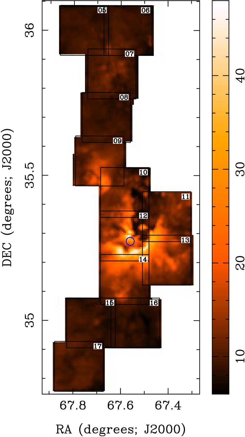
Figure 4 shows a map of the spatial distribution of the 12CO excitation temperatures in the surveyed region. Over the vast majority of the cloud, Tex is found to be in a narrow range around 10 K as expected for gas heated by cosmic rays and cooled by molecular lines (Goldsmith & Langer, 1978; Bergin & Tafalla, 2007). Higher temperatures are found in the southern part of the region. The highest excitation temperatures approach 40 K and are found within the bright filamentary ridge southwest of the LkH 101 cluster (see figure) suggesting that the cluster is providing additional heating of the gas in that area.
The optical depths of 13CO(2-1) () and C18O(2-1) () were calculated assuming LTE from:
| (4) |
Here Tex for both transitions was taken to be that derived for 12CO(2-1). The probability density distribution of opacities for 13CO peaks around 0.5 with the majority (87%) of pixels appearing to be relatively optically thin (i.e., 1). For C18O the distribution peaks around 0.2, significantly less than that for 13CO (as expected), and with 1 for essentially all pixels in the map.
We followed Pineda et al. (2010) in calculating both the 13CO and C18O column density using Eq.5 for J=2-1 transition333We noticed the typo in equation (18) in Pineda et al. (2010), as pointed out by Ripple et al. (2013). The rotational constant B0 and the Einstein coefficient A2→1 are taken from an online database444http://home.strw.leidenuniv.nl/~moldata/CO.html. The partition function Q is estimated by Eq.6, which is accurate to 10 percent for T 5 K (note that in our data, Tex 5 K everywhere, as shown in Figure 4).
| (5) |
| (6) |
We note that sub-thermal excitation for the optically thin 13CO(2-1) and C18O(2-1) lines might be expected to be a concern in low extinction regions of the cloud where number densities may be lower than the critical density for thermal (LTE) excitation ( 3 104 cm-3). This could lead to underestimates of the CO column densities in the outer regions. However, since the studied area here is dominated by relatively high extinction (AV 3-4 magnitudes) we expect that the effects of any sub-thermal excitation are minimized. We can roughly estimate the magnitude of this effect using the RADEX, non-LTE, radiative transfer code (van der Tak et al., 2007). We find that with cm-3, Tgas 10 K, and W(13CO) 2.5 K km s-1, NRADEX 2.0 NLTE.
4. Discussion
4.1. CO Column Densities and Visual Extinction
4.1.1 13CO and C18O Abundances
Since our measurements of CO column densities and dust extinction are set to the same angular resolution and spatial grid, we are in a position to directly compare the two data sets. We note here that the angular scale of a pixel is 19, corresponding to a spatial scale of 0.04 pc ( 8000 AU) at a distance of 450 pc (Lada, Lombardi, & Alves, 2009).
Assuming a constant gas-to-dust mass ratio, (N(H)/AV =1.881021 cm-2 mag-1) (Bohlin et al., 1978; Rachford et al., 2009; Pineda et al., 2008), the CO abundance can be expressed as: [CO] = N(CO)/N(H) = N(CO)/[AV()]. For optically thin emission lines, such as 13CO and C18O, we expect the gas column density to increase linearly with AV, provided the cloud is characterized by a constant CO abundance (e.g., Lada et al., 1994; Alves et al., 1999). In Figure 5 we plot the molecular column density vs. extinction at each pixel in the mapped region for 13CO (a) and C18O (b), respectively. Contrary to our simple expectations, each plot exhibits considerable scatter with only weak correlations between gas and dust column densities. If the gas in the CMC were characterized by a single, constant abundance, the relation between its column density and extinction would consist of a single straight line in each plot. At fixed AV there would be only small scatter in N(CO), which is clearly not the case. For instance, at AV 20 mag the ratio between the highest and lowest values of N(13CO) and N(C18O) is 10 for each isotope. Clearly, the two plots suggest strong spatial variations in abundances of these two species across the cloud.
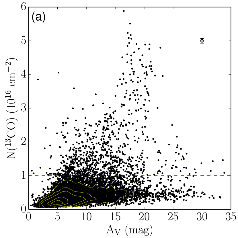
On closer inspection of Figure 5 one can almost make out two significant branches (correlations) of pixels in both plots. First, a large group of pixels in each plot (below the blue dashed line, i.e., N(13CO) 1.01016 cm-2, N(C18O) 1.01015 cm-2) display an almost constant, low column density across a wide range of AV. This flat relation between the two quantities indicates a trend of decreasing molecular abundance ([13CO] and [C18O]) from low to high AV pixels. Second, another group (above the blue dashed line) of pixels is characterized by gas column densities that appear to rise more or less linearly with extinction to very high column density at AV 20 mag (1.01016 cm-2 N(13CO) 6.01016 cm-2, 1.01015 cm-2 N(C18O) 6.01015 cm-2), indicating a more or less uniform molecular abundance with depth into the cloud for this group of pixels. These branches likely mark two limiting extremes of spatially dependent variation in the chemical conditions within the CMC.
Spatial variations in 13CO abundances have been reported previously in a few other molecular clouds, although in these clouds the variations appear less pronounced than found here. For the Perseus molecular cloud, Pineda et al. (2008) found generally tighter correlations of 13CO column density with extinction than found here, although they explored the correlation at much lower extinctions (i.e., AV 10 mag) than in this study. Nonetheless, over this lower extinction range they did find measurable variations (at the 40% level) in the abundances with position across the cloud. For the Orion A molecular cloud, Ripple et al. (2013) measured abundances at both low and high extinction and found more significant positional variations in the 13CO abundance across the cloud than observed in Perseus (Pineda et al., 2008). At AV 20 mag, N(13CO) in Orion A was found to vary by about a factor of 4 between various locations in the cloud. Further, Ripple et al. (2013) were able to associate these positional variations in abundance with positional variations in the physical conditions within the cloud. At the lowest extinctions (AV 3 mag), where there is not enough 13CO to self-shield against UV dissociation, they found extremely low 13CO abundances with significant (factor of 8) spatial variations. At intermediate extinctions (3 AV 10 mag), where self-shielding is considerably more effective, higher abundances were found with modest (factor of 2) spatial variations. At the highest extinctions they observed the highest abundances but also the largest spatial variations in abundances across the cloud. This latter regime included cold portions of the cloud where CO depletion depressed the abundances as well as hot regions heated by young stars where CO desorption produced enhanced CO abundances.
4.1.2 Mapping Spatial Variations in CO Abundances
The molecular abundance is regulated by the physical and chemical conditions in the GMC. For instance, the gas-phase molecules can condense onto dust grains to form ice mantles, and the molecules on grain surfaces can be returned to the gas via thermal evaporation (e.g., van Dishoeck et al., 1993; Caselli et al., 1999). These processes are tightly linked to the local temperature (especially the dust temperature), and are responsible for setting the gas-phase molecular abundance. At low extinctions where column densities of dust and gas are low, abundances are very sensitive to FUV radiation which can drive volatile chemistry via processes of fractionation and selective photodissociation (Lada et al., 1994; Röllig & Ossenkopf, 2013). The large scatter in Figure 5 could plausibly be caused by strong variation of such physical/chemical conditions in different sub regions of the surveyed area of the cloud. If this is the case, we would expect to observe a tighter correlation between column density and AV if we restricted the plots to cover smaller spatial areas within the surveyed region, since the physical conditions in such smaller regions would be expected to be more uniform. Indeed, Ripple et al. (2013) demonstrated the connection between such physical conditions and spatial CO abundance variations in the Orion cloud.
| Tile | slopeaa Linear regression results from Figure 6. In tiles 11-14, the fitting is performed over the entire AV range. In the rest of tiles, the fitting is up to AV = 10 mag. The r-value (Pearson coefficient) is an estimation of correlation coefficient. | r-valueaa Linear regression results from Figure 6. In tiles 11-14, the fitting is performed over the entire AV range. In the rest of tiles, the fitting is up to AV = 10 mag. The r-value (Pearson coefficient) is an estimation of correlation coefficient. | |
|---|---|---|---|
| (K) | (1016 cm-2 mag-1) | ||
| 01 | 9.21 | 0.014 | 0.42 |
| 02 | 9.31 | 0.027 | 0.65 |
| 03 | 8.30 | 0.031 | 0.64 |
| 04 | 8.52 | 0.025 | 0.50 |
| 05 | 9.14 | 0.024 | 0.57 |
| 06 | 9.23 | 0.018 | 0.43 |
| 07 | 9.99 | 0.046 | 0.64 |
| 08 | 9.19 | 0.037 | 0.55 |
| 09 | 12.3 | 0.034 | 0.37 |
| 10 | 12.3 | 0.066 | 0.67 |
| 11 | 13.1 | 0.148 | 0.80 |
| 12 | 19.6 | 0.193 | 0.76 |
| 13 | 16.5 | 0.204 | 0.91 |
| 14 | 16.9 | 0.102 | 0.62 |
| 15 | 9.07 | 0.059 | 0.75 |
| 16 | 8.65 | 0.054 | 0.64 |
| 17 | 9.66 | 0.022 | 0.64 |
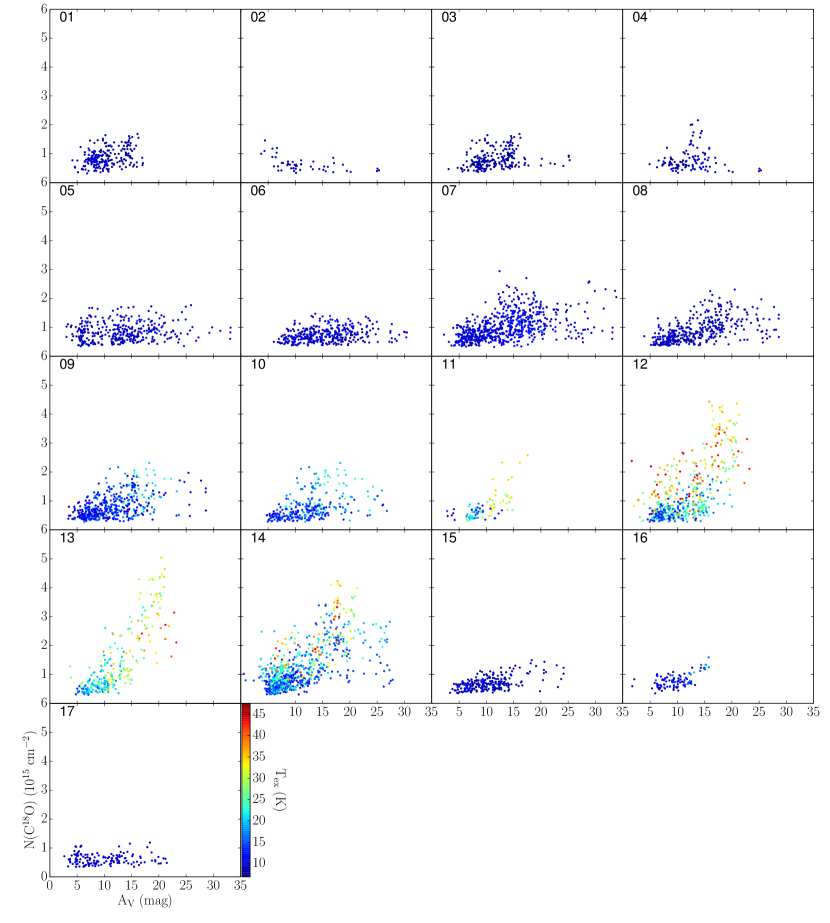
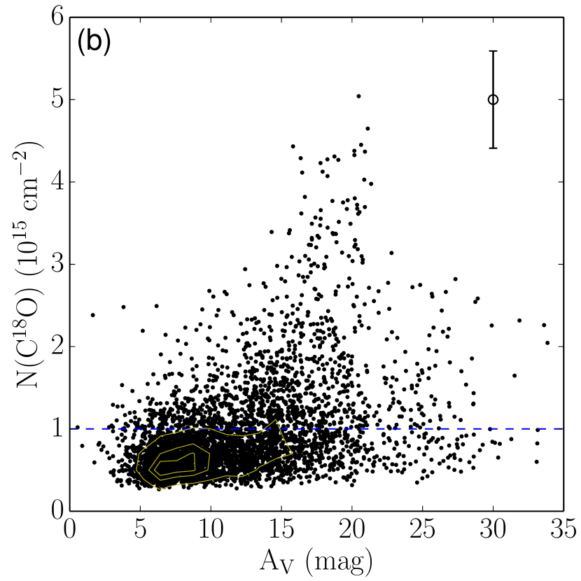
In order to examine the distributions of N(13CO) and N(C18O) versus AV on smaller spatial scales, we constructed these relations for each individually observed mapping tile (c.f. Figures 1 and 2). In Figures 6 and 7 we plot the results for 13CO and C18O, respectively. In the individual plots contained within these figures we indeed see a significant reduction in scatter compared to that characterizing Figure 5. More importantly, there is very strong spatial variation in the relation between extinction and CO column density across the surveyed region of the CMC. This is evident in Figure 6 where we plot linear fits to the data. The results of the fits are shown in Table 2 where the slopes vary by nearly an order of magnitude across the cloud. This is also readily apparent in Figure 7 where the axes on the plots have the same scaling and especially clear on close inspection of Figure 6 where the scale of the vertical axis ranges by as much as an order of magnitude between the various tiles. These spatial variations in N(13CO) and N(C18O) give rise to the large dispersion in these quantities in the merged relation constructed for the entire observed region as in Figure 5. Despite the variation in the range of column densities at different locations across the cloud, the range in extinction spanned by the observations in all the plots is very nearly the same. The large variation of column density of 13CO and C18O with dust extinction confirms that the abundances of the two isotopologues exhibit large spatial variations. Consider Figure 6. The tiles can be placed into two groups, one containing tiles 1-10 and 15-17, and the other consisting of tiles 11-14. In the former group, N(13CO) rarely exceeds a 5-6 1015 cm-2, while in the latter group N(13CO) can reach values as high as 3-5 1016 cm-2 over the same extinction range. The N(C18O) plots in Figure 7 exhibit similar behavior.
4.1.3 The Relation between Gas Temperature and CO Abundances
From comparison of Figures 7 and 6 with Figure 4 we see that the tiles (11-14) with the largest values of CO column density spatially coincide with the region of elevated 12CO excitation temperature. Since the 12CO(2-1) line is generally so optically thick, and since our sampled region preferentially contains high column density (AV 3-5 mag) gas, sub-thermal excitation of 12CO is unlikely. Therefore the excitation temperature map traces the gas kinetic temperature and the distribution of the molecular abundances [13CO] and [C18O] are tightly related to local physical conditions, in particular the gas kinetic temperature. As a further test of the connection between column density and temperature we have color-coded the points in Figures 6 and 7 according to the gas temperature in each individual pixel. Inspection of the figures shows that the pixels with the highest gas temperatures (Tex 15 K) are also the pixels with the largest CO column densities. Pixels with low gas temperatures (Tex 15 K) rarely reach high CO column densities, independent of extinction. These correlations imply that the abundances of 13CO and C18O are physically related to the gas temperature distribution.
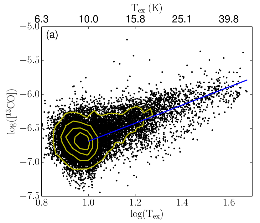
To examine more directly the relation between the molecular abundances and the gas temperature, we plot the log([13CO]) - log(Tex) relation and log([C18O]) - log(Tex) relation in Figure 8. Both molecular abundances show dependence on Tex, although [13CO] is apparently sensitive to Tex over a larger range of temperature than [C18O]. This confirms that [13CO] and [C18O] are both regulated by gas temperature, but over different ranges of temperature in the extinction range (3 mag AV 25 mag) we observed. To quantify the relations, we empirically fit a power-law functions to the unbinned data for both correlations. Tex is derived from the 12CO line, which has very good SNR. Since the noise of extinction map is relatively small, i.e., 0.05 mag for Av10 mag and 0.1 mag for Av10 mag, uncertainties in the abundances are dominated by the noise in the molecular line data.
The fits were performed over different ranges of Tex for the two lines: Tex 10 K for 13CO and Tex 17 K for C18O. The low temperature cutoffs were empirically chosen, by inspection, to correspond to the ranges where the relations appeared to be linear. However, it did not escape our attention that the low temperature cutoff for C18O corresponds to the CO sublimation temperature of 17 K (van Dishoeck & Black, 1988), and as discussed later this may not be coincidental. The linear regression gave the following results: [13CO] T with correlation coefficient = 0.66; [C18O] T with correlation coefficient = 0.34. We performed a test on the power-law model for [13CO] - Tex and [C18O] - Tex relations. The is calculated using:
| (7) |
where O and E stand for observed and modeled [CO] (calculated from the fitted power-law), respectively, and the local standard deviation derived in a 2 K bin enclosing the data. At a significance level of 0.05, the fitted power-law models for [13CO] - Tex and [C18O] - Tex relations are acceptable, and the per degree of freedom are 1.02 and 1.06 for [13CO] and [C18O], respectively, meaning the fit is reasonable. The implications of these results will be discussed in the next two sections of the paper.
4.1.4 Molecular Depletion and Desorption
We argue here that the dependence of the 13CO and C18O abundances on gas temperature shown in Figure 8 is a result of the combined effects of gas depletion and desorption in the CMC. Theoretical considerations suggest that sticking of CO onto dust grains can remove the molecule from gas-phase very efficiently within cold (T 17 K) and dense (n(H2) 104 cm-3) regions of molecular clouds (see, e.g., van Dishoeck et al., 1993). Indeed, compelling observational evidence for reduction of [C18O] has been reported for numerous cold (T 10 K) and high extinction (AV 10 magnitudes) regions of molecular clouds (e.g., Lada et al., 1994; Alves et al., 1999; Caselli et al., 1999; Kramer et al., 1999; Bergin et al., 2001, 2002). Both the radial stratification of the clouds (e.g., Alves et al., 1998, 2001; Bergin et al., 2001) and the presence of emission from high dipole molecules such as NH3 from such regions indicate that they likely correspond to sufficiently high gas volume densities (104 cm-3) to promote CO condensation onto grain surfaces.
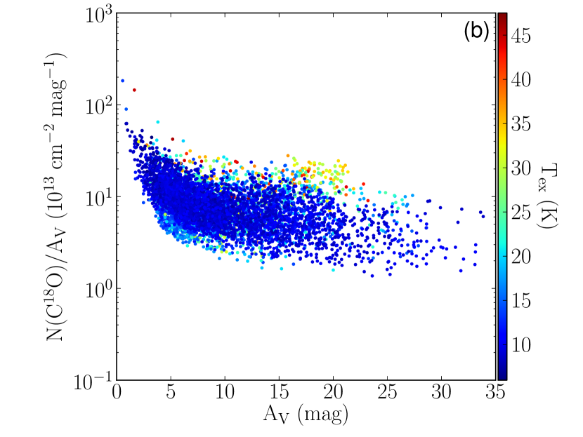
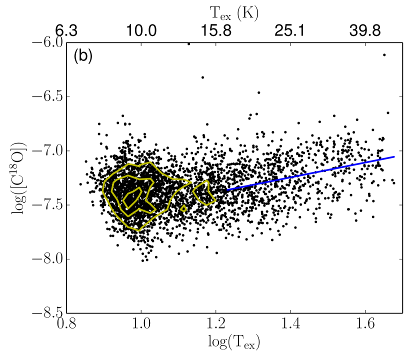
In Figure 9 we plot the relation between (a) 13CO and (b) C18O abundance and extinction in the CMC. Although there is a large scatter in both relations, it is clear that the abundances of the two species decline with extinction in a manner consistent with similar abundance reductions seen in other molecular clouds and suggestive of CO freeze out onto grain surfaces in the interior regions of the cloud. If this decline in abundances at high extinctions is due to freeze out, we also expect the reduction of the gas-phase abundances to be occurring in the coldest regions of the cloud. In Figure 9 the points are color-coded by the gas temperature and we see both a preponderance of cold gas in the cloud, and a prominent decrease in abundance with extinction for the cold pixels, while the warm pixels show no decrease. This supports the hypothesis that the decline in abundances with extinction in cold regions is largely due to depletion. Of course, depletion requires low dust temperature and our analysis has been based on measurements of gas temperature. Gas temperature generally tracks dust temperature (e.g., Forbrich et al., 2014) but direct observations of dust temperature would make for a more compelling case. Fortunately, published maps of dust temperature for the CMC based on Herschel observations exist (Harvey et al., 2013). Comparison with our maps shows generally good agreement between the gas and dust temperature spatial distributions. In particular, in the cold regions away from LkH 101 (corresponding to our tiles 01-09 and 15-17, respectively), the median Td 14.5 K and the minimum Td 10 K (Harvey et al., 2013), far below pure CO ice sublimation temperature ( 17 K, van Dishoeck et al., 1993). Under such conditions, Bergin et al. (1995) showed a relatively short CO depletion timescale, 106 yr. So with Td 10 K and = 104 cm-3, CO would unavoidably deplete. This is consistent with the reduction of CO abundance we observe in the cold, high extinction regions in the CMC.
At the higher gas temperatures (T 17 K) we would expect that thermal evaporation (desorption) of the gas from the grain surfaces releases any trapped CO and increases its gas phase abundance relative to the cold regions of the cloud. Indeed, that is what is clearly shown in Figure 8 where the observed abundances increase with increasing gas temperature. The warmest CO gas in our surveyed region is found in four contiguous tiles (11-14) that are in close proximity to the massive star LkH 101 and its associated cluster (shown as the blue circle in Figure 4). The CMC dust temperature map from Harvey et al. (2013) (see their figure 4) shows a vast region of high dust temperature (Td 28 K) near LkH 101, which coincides with the positions of tiles 11-14 in our observation. It is in this warm area that the CO abundances appear to be at their highest. CO thermal evaporation is caused by high dust temperature. For instance, Bergin et al. (1995) reported that shortly after a “star turns on”, the dust temperature reaches Td = 25 K ( = 104 cm-3, Tgas = 20 K), and all CO is in the gas phase within 100 yr. The abundance enhancement near LkH 101 is likely caused by hot dust heated by the cluster. Over most of the rest of the cloud Harvey et al. (2013) find Td 10 - 14 K. In these regions the gas temperatures are also found to be near 10 K and a significant amount of CO should be locked in ice mantles on the dust grains at least at the highest extinctions (also see Bergin et al., 1995). These considerations suggest that the variation of [13CO] and [C18O] in the CMC is mostly regulated by the chemistry of depletion and desorption which in turn is driven by the (dust) temperature distribution.
Recently, Ripple et al. (2013) have reported similar results for the Orion A molecular cloud. They divided that cloud into 9 spatial partitions (1-9) and considered regions within those partitions with extinctions, AV 5 magnitudes, similar to those studied here for the CMC. They found that in regions with 5 AV 10 magnitudes, N(13CO) was generally linearly correlated with AV. However, in those partitions (2, 3 & 4) that also contained higher extinction material and were characterized by mean gas excitation temperatures that were below 22 K, the N(13CO)-AV relation became flat above AV 10 magnitudes. On the other hand, in two partitions (5 & 6) with both high extinctions and high mean gas excitation temperatures (Tex 26-33 K), N(13CO) continued to rise above AV 10 magnitudes. Ripple et al. (2013) posited that this behavior of N(13CO) with extinction was a result of depletion/desorption effects at AV 10 magnitudes. Our results for the CMC are certainly consistent with those of Ripple et al. (2013) for Orion A. In this respect, the physical/chemical conditions in the Orion and the CMC appear to be quite similar. The spatial variations in abundances of the rarer isotopes of CO are largely determined by depletion/desorption effects due to spatial variations in dust (and gas) temperatures resulting from localized star formation activity within the clouds.
4.1.5 The 13CO-to-C18O Abundance Ratio: Influence of UV photodissociation
In the outer, lower extinction regions of molecular clouds, FUV radiation is expected to play a role in cloud chemistry (e.g., van Dishoeck & Black, 1988; Visser et al., 2009). In low extinction regions (i.e., AV 3 mag) fractionation of 13CO can increase its abundance relative to 12CO. At somewhat higher extinctions (AV 5 mag) selective photodissociation of C18O is likely to occur due to differences in self-shielding of the FUV intensity at the dissociation wavelengths for the various CO isotopes. The more abundant 12CO and 13CO isotopes are effectively self-shielded at relatively low extinctions (AV 1 magnitudes) but because the dissociation wavelength of C18O is slightly shifted compared to 12CO and 13CO, and its abundance is relatively low so it is not as effectively self-shielded as the main isotopes, FUV radiation can penetrate deeper into the cloud and dissociate the C18O (Visser et al., 2009). Since our surveys cover relatively high extinction regions (AV 5 mag) we would not necessarily expect selective photodissociation to strongly effect the 13CO to C18O abundance ratios. However, earlier studies of Lada et al. (1994) and Shimajiri et al. (2014) suggest that the effects of selective photodissociation may be present at much higher extinctions.
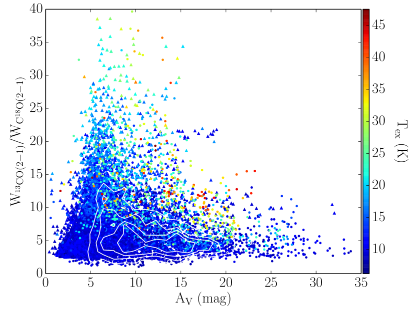
In Figure 10 we plot the ratio of integrated intensities, W(13CO)/W(C18O), as a function of extinction. This ratio is proportional to the abundance ratio for the two species for optically thin lines. It has been shown to be sensitive to the effects of UV radiation on cloud chemistry and abundances (e.g. Lada et al., 1994; Shimajiri et al., 2014). For a solar abundance and optically thin lines, the ratio should be equal to about 5.5 and one would expect the points to scatter around this value, independent of extinction, provided the cloud is characterized by a constant relative abundance throughout and that the excitation of the two species is not too different. Although at lower extinctions (AV 15 magnitudes) there indeed appears to be no obvious correlation between this ratio and extinction, the observed values scatter over an enormous range ( 0 - 40). The highest values of the ratio exceed the solar value by nearly an order of magnitude555We note here that in the outer regions of the cloud, C18O is often undetected while 13CO is still quite strong. Because C18O is in the denominator, the ratio is very sensitive to noise in the outer regions. However, at all locations 13CO detections exceed the 5 level. To reduce the scatter in the plot due to non-detections of C18O we set the C18O integrated intensity equal to 2 for those pixels where W(C18O) is below 2 . We represent the resulting lower limits on the calculated ratio as triangles in the plot (see figure).. In contrast, at high extinctions (AV 15 magnitudes) the relation is relatively flat with a relatively low dispersion, as might be expected for a constant abundance ratio, and is centered at a value (approximately 4.5) near but somewhat less than the solar value. This behavior does not appear to depend on gas temperature (see figure) and thus is not likely a result of depletion or desorption processes on grains. It is more likely indicative of an active chemical processing of C18O by FUV radiation in regions where AV 15 magnitudes. The scatter in Figure 10 is so large at these extinctions because the relative abundance of 13CO and C18O is highly unstable possibly due to the stochastic variations in FUV flux resulting, in turn, from such factors as the cloud structure and geometry and nature of the external radiation field.
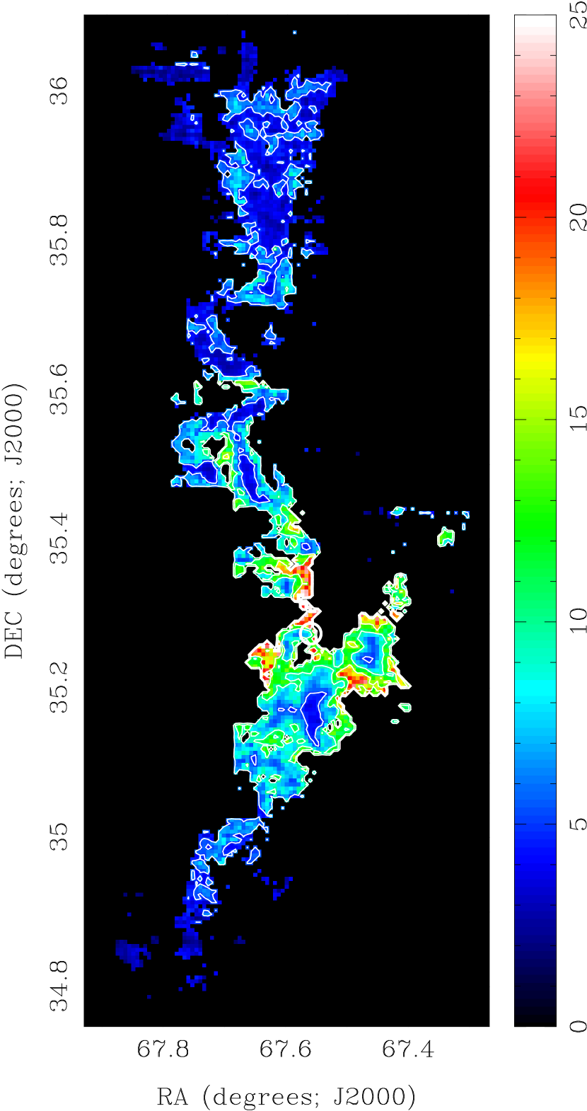
In Figure 11 we show a map of the distribution of the integrated intensity ratio over the southern portion of the CMC. Examination of this map shows systematically increasing values of the integrated intensity ratio at the edges of the cloud with the material nearest the star LkH 101 exhibiting the largest center to edge increases in the ratio. This latter region appears to contain a well developed photon dominated region (PDR) while the dense cloud material to the north is much more quiescent in this regard. In their study of the Orion cloud Shimajiri et al. (2014) reported averaged values of the 13CO to C18O integrated intensity ratio ranging from about 10 to 17 in the seven PDRs they observed in that cloud. Moreover they also found the variations in this ratio to be linked to variations in the external FUV radiation field.
In the inner, higher extinction regions of the CMC, where FUV photons cannot penetrate, the abundances are more chemically stable and apparently somewhat below the solar value. Our observations do indicate, however, that FUV photons are present at relatively large (projected) depths (AV 15 magnitudes) in the cloud confirming results from earlier studies (e.g. Lada et al., 1994; Shimajiri et al., 2014).
We now address the earlier observation that the relations between the CO abundances and temperature (Figure 8) show positive correlations but over different temperature ranges. One might have expected both 13CO and C18O molecules to show abundances that increased with temperature over similar temperature ranges, since their binding energies are very similar. However, the difference may result from the effects of selective UV dissociation of C18O.

In the CMC we also find Tex to be correlated with AV in regions where warm gas is present. Figure 12 displays the relation between Tex and AV for the warm tiles (11-13) in our map. Although the scatter is large at high AV, there is no doubt of a strong trend between the two quantities with Tex AV. Interestingly in this region the temperature reaches the CO sublimation temperature at roughly AV 6-7 magnitudes. Therefore it is possible that, even though C18O is being evaporated from grains at AV 6 magnitudes, (where Tex 17 K) it is also being selectively photodissociated by deeply penetrating UV radiation until depths of AV 15 magnitudes. For larger values of AV, dust absorption effectively removes the dissociating UV radiation and higher gas (dust) temperatures associated with this region liberate more C18O from grain surfaces. Indeed, the C18O abundances at these higher extinctions and temperatures may reach levels that also allow some C18O self-shielding. Consequently, C18O does not reach the expected levels of increased abundance due to evaporation from grains until cloud depths are sufficient to shield the molecule from UV radiation. Because of its higher abundance, 13CO self-shields at much lower cloud depths and the effects of its increased abundance, due to evaporation from grains, are observed at lower extinctions (and corresponding lower temperatures) than C18O.
4.2. X(CO) on Sub-Parsec Scales
Even though H2 is the dominant constituent of molecular clouds, 12CO emission is the most accessible tracer of such gas in the ISM. It is often the only molecular tracer that can be readily detected in distant clouds and galaxies and consequently has been used to estimate the mass of the molecular component of the ISM in these systems (e.g. Bolatto et al., 2013). To make such estimations requires knowledge of the so-called X-factor, that is, the CO conversion factor,
| (8) |
The standard determination of this factor is via use of virial theorem techniques (e.g. Solomon et al., 1987). However, the most straightforward way to determine the X-factor is by comparing direct measurements of CO and AV on sub-parsec scales in local clouds. Traditionally this is accomplished by measuring the slope of the correlation between the two quantities at low extinctions (AV 5 mag) where the CO appears to be effectively thin (e.g. Dickman, 1978; Frerking, Langer, & Wilson, 1982; Lombardi et al., 2006). We adopt a slightly different approach and use all our observations to compute a global or average X-factor for the CMC cloud, that is, = / 2.531020 cm-2 (K km s-1)-1. This value is 25% larger than the standard Milky Way value but within the range of values derived for individual molecular clouds in other studies (e.g. Bolatto et al., 2013). Another approach is to derive the on-the-spot XCO, that is, we evaluate Equation 8 at each pixel in our map and obtain = 3.11020 cm-2 (K km s-1)-1. The former XCO is equivalent to the latter weighted by the integrated intensity.
However, both recent observational studies (Pineda et al., 2008, 2010; Bieging et al., 2010; Ripple et al., 2013; Lee et al., 2014) and numerical simulations (Shetty et al., 2011a, b) have shown that XCO can be strongly dependent on local physical conditions. Since the CMC displays a wide range of physical conditions (e.g. temperature, star formation activity and spatially variable CO abundances), it would be interesting to measure both XCO and its internal variation on sub-cloud, sub-parsec scales.
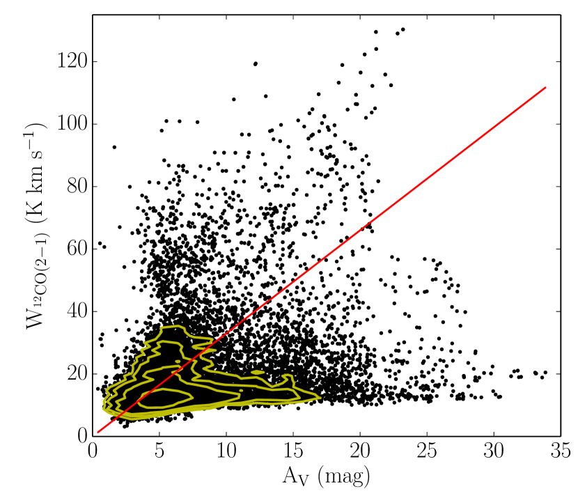
To do this we first performed the traditional pixel-by-pixel comparison between W and AV for the entire surveyed region, as shown in Figure 13. Assuming a constant gas-to-dust ratio N(H2)/AV =9.41020 cm-2 mag-1 (Bohlin et al., 1978; Rachford et al., 2009; Pineda et al., 2008) and a constant line integrated intensity ratio WCO(2-1)/WCO(1-0) = 0.7, XCO(1-0) is inversely proportional to W/AV in the plot. In the Milky Way disk, the typical value is XCO(1-0) 21020 cm-2 (K km s-1)-1 (e.g., Bolatto et al., 2013). This implies a reference value AV/WCO(2-1) 0.30 (K km s-1)-1 mag. We plot a red line indicating this reference value in Figure 13, with a slope of WCO(2-1)/AV 3.3 (K km s-1) mag-1. At fixed AV, a point above this line indicates a smaller XCO(2-1), and vice versa.

We can see significant scatter in this plot indicating significant spatial variations in XCO(2-1) on pixel or sub-parsec spatial scales. In order to investigate the spatial dependence of XCO(2-1), we determined the W–AV relation in each individual tile of our CO survey, following Section 4.1.2. These relations are shown in Figure 14. There are several familiar features of these plots that are similar to what we have seen in Figure 6, i.e., less scatter in the relations within the individual tiles, systematic spatial variations in the W – AV relation across the cloud, and good correlation between high W and high gas temperature (Tex 15 K).
The general similarity666 By “similarity” we mean the hot tiles 11-14 show steeper slopes than the cold tiles in both W - AV (Figure 14) and N(13CO) - AV (Figure 6) relations. The apparent relative differences between the the cold tiles in Figure 6 compared to Figure 14 is a result of different y-axis scaling. in the behavior of W and N(13CO) with extinction is perhaps surprising given that the 12CO emission is very optically thick while 13CO emission is considerably less thick and mostly optically thin. Since N(13CO) is proportional to W, consider that in this situation , while , where is the line width of the corresponding spectrum. Unlike W, W has no dependence on or column density, but it is proportional to Tex, the gas excitation temperature.
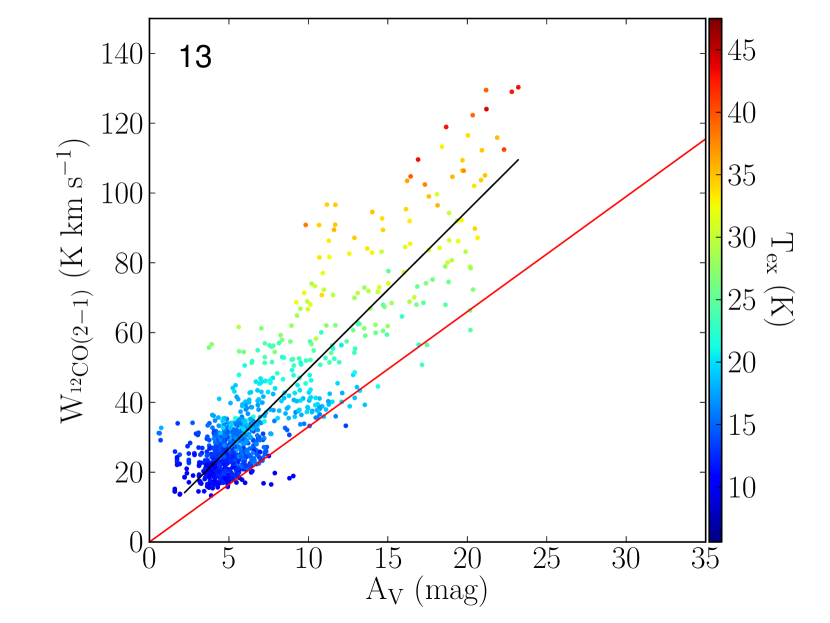
Particularly interesting in this regard is the behavior of W in tile 13 near where the embedded cluster is heating the cloud. Here, there appears to be a clear linear relation between W and AV to the highest measured extinctions ( 25 magnitudes) despite the fact that the 12CO emission in this region of the cloud is so saturated that it is self-reversed (see Figure 2). Because the CO emission is so optically thick, this behavior must be primarily the result of the gradient of Tex with AV observed in this region of the cloud (see Figure 12) . This is also evident in Figure 15 which shows an expanded view of the W–AV relation for tile 13. We can clearly see a temperature gradient in the distribution of color-coded points from low to high AV. Both W(CO) and T increase by a factor of 5-6 from low to high AV. This indicates that the temperature gradient accounts for the bulk of the change in W(CO) with AV in this region. Of course, other factors could contribute to the increase in W(CO) such as an increase in velocity dispersion with temperature, or even increased [CO] due to desorption as with C18O and 13CO as discussed previously. We do find some evidence for a marginal (35%) increase in the velocity dispersion of the hot gas, but its magnitude is far from sufficient to account for the increased () measures of W(CO). A desorption induced increase in CO abundance most certainly has occurred in the hot gas, and although the 12CO line is very optically thick, we might expect that additional photons could leak out in the line wings and possibly increase the measured velocity dispersion. But as we already remarked, this effect cannot be significant since the change in peak brightness is observed to be comparable to the change in W(CO) and substantially larger than changes in the velocity dispersion.
Consequently, in the set of tiles near the massive star LkH 101 (11-14) we conclude that heating of CO enhances W in a manner that induces a positive correlation with extinction despite the fact that the emission is saturated. These observations suggest that heating by OB stars produces gradients in the excitation temperature of the CO emitting gas such that in warm regions W(12CO) is proportional to AV and thus to N(H2) over a wide range of extinctions. This, in turn, indicates that a single, meaningful X-factor can be derived for these hotter regions using the observations. In Figure 14, tile 13 shows the best correlation between W(12CO) and AV. We performed a linear regression for tile 13, which is shown in Figure 15. Our result implies
in this tile over the range 3 mag AV 25 mag. From the average of the individual, on-the-spot, XCO values in tile 13 we find XCO , in excellent agreement with the value derived from the linear regression. This clearly supports the idea of a constant value in the hot gas. The derived value is less than both that found for the global average of the CMC and the value () usually adopted for the Milky Way.
This result would suggest that in regions heated by OB stars (e.g., as HII regions, extragalactic starbursts, etc.), reasonably accurate gas masses could be derived using a standard X-factor analysis with a single value of the X-factor. Unfortunately it is not at all clear how one would predict the appropriate value to use in all situations.
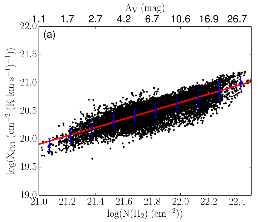
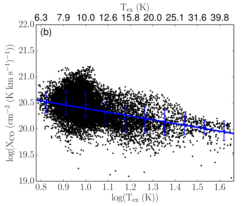
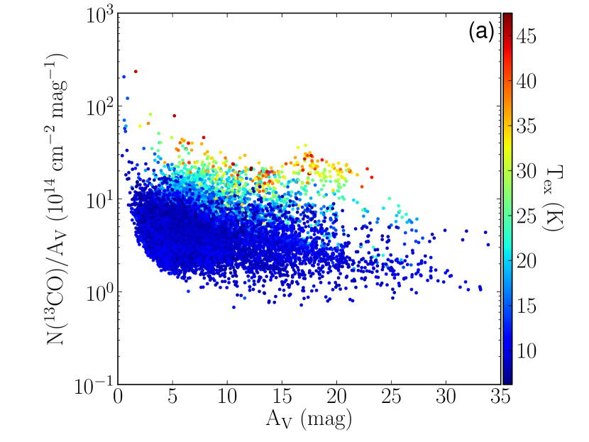
However some clues may be found in the analysis of the regions away from OB stars, where there is only ambient heating of the gas from cosmic rays and the general galactic UV radiation field. Here we observe no correlation between W and AV at modest to high extinctions (i.e., AV 3-5 mag). This behavior is due to the fact the 12CO line is almost always saturated at high extinctions and the cold gas is very nearly isothermal. Consequently, these cold, quiescent regions, are not characterized by a single empirical X-factor, instead, the X-factor systematically increases with extinction and, in the CMC, is almost always larger than the Milky Way value. This is shown in Figure 16a where we plot the relation between the on-the-spot X-factor and AV for the regions of the cloud not heated by the cluster (i.e., tiles 1-10 and 15-17). As expected there is a clear correlation and a linear least-squares fit to the unbinned data finds that XCO N(H2)0.7. For the cold tiles we find XCO = 3.4 1020 . The (constant) X-factor in the hotter regions (e.g., tile 13) has a value considerably lower than those in the cold regions, suggesting that XCO may also increase with decreasing gas temperature within the cloud. Such a trend is clearly evident in our observations and is shown in Figure 16b where we plot the relation between the on-the-spot XCO and Tex for the entire cloud. A linear least-square fit to the (binned) data gives, XCO 2.0 1020(Tex/10)-0.7 . In this instance we chose to fit the binned data to give greater weight to high temperature measurements. A fit to the unbinned data gives a slightly steeper slope (-0.9 vs. -0.7).
The observed inverse correlation between XCO and Tex is potentially interesting. It suggests that differences between globally averaged X-factors derived for different clouds could be a result of variations in the relative amounts of hot and cold gas within the clouds, provided their velocity dispersions are similar. Active star forming clouds with OB stars and HII regions, such as Orion, might be expected to have average X-factors that are lower than more quiescent clouds, such as the CMC. Indeed, Digel et al. (1999) derive XCO 1.35 1020 for the entire Orion complex from ray data, in agreement with recent determinations using CO (Ripple et al., 2013). Moreover, ray observations of Orion with the Fermi satellite by Ackermann et al. (2012) found that in the (cold) regions removed from the OB stars and HII regions, XCO 2.2 1020 , while in the (hotter) parts of the cloud complex associated with the HII regions, XCO 1.3 1020 , very similar to what we find in the California cloud. For the Taurus cloud, which has no OB stars or HII regions, Pineda et al. (2010) find XCO = 2.1 1020 from CO observations of that cloud. A relatively high value (2.54 1020 ) for XCO was also derived from Planck observations of high latitude diffuse and presumably cold, CO gas (Planck Collaboration et al., 2011). We noted earlier that the global X-factor for the CMC was 25% higher than the Milky Way value and this is may be due to the relatively large tracts of cold regions included in the average for the CMC. Of course, variations in velocity dispersions between clouds could also contribute to the variation in their observed X-factors. However, we would expect similar velocity dispersions to characterize gravitationally bound or virialized clouds of similar mass and size. Moreover, since the average column densities of molecular clouds are also constant (e.g., Larson, 1981; Lombardi et al., 2010), we would expect XCO T for such clouds. As recently pointed out by Narayanan & Hopkins (2013), Galactic GMCs are characterized by very similar physical properties resulting in X-factors that span a relatively narrow range of values. They suggest that this is a result of the competition between stellar feedback and gravity that is necessary to maintain the relative stability of these objects. Here we are suggesting that variation within that narrow range of observed XCO may be due to variations in the relative fractions of hot gas in these clouds. This hot gas, of course, is a direct product of the amount of stellar feedback the clouds are experiencing. Resolved maps of the internal X-factor distribution in additional clouds would be useful to determine the relative contribution of temperature to the derived values of XCO within GMCs in general and could directly test this idea.
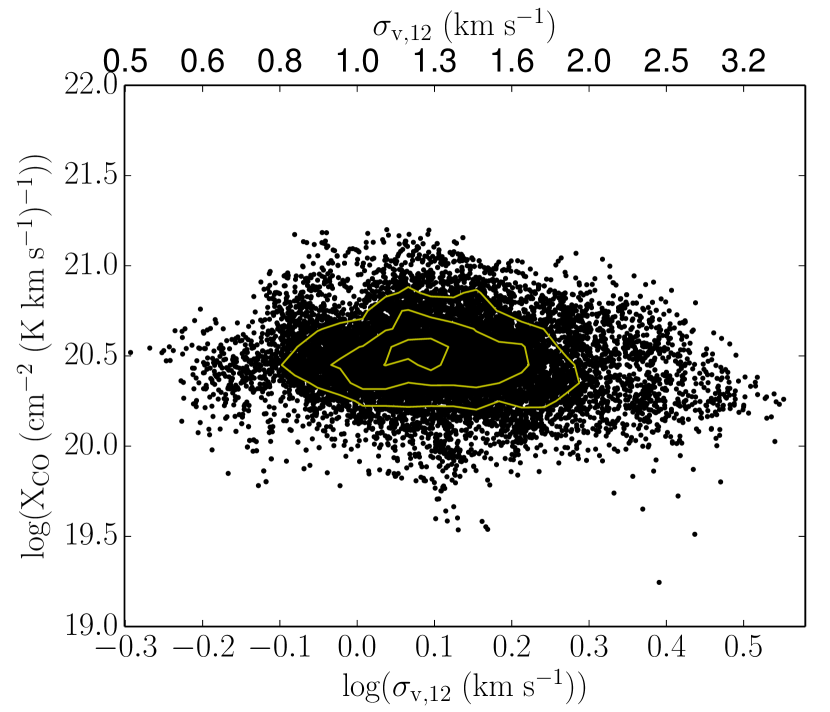
Absent of such additional data, it is instructive to compare our observations to recent simulations of turbulent cloud evolution that resolve synthetic clouds and derive the internal spatial distribution of the X-factor (Shetty et al., 2011a, b). These simulations are thus directly comparable to observations such as ours. The Shetty et al. simulations include chemical evolution and radiative transfer to enable predictions of CO line emission. However, the calculations do not include gas-dust chemical interactions and are thus not relevant to our earlier findings or discussion regarding [13CO], [C18O], and W(13CO)/W(C18O). But since 12CO is so optically thick we safely assume that effects of depletion/desorption are not important for our X-factor determinations and thus comparisons with these models are appropriate. Because the Shetty et al. simulations do not incorporate stellar feedback, the most appropriate comparison will be with our data in the regions of the CMC away from the embedded cluster (all tiles excluding 11-14). The simulated cloud of Shetty et al. (2011b) whose physical conditions match most closely those of typical GMCs is characterized by a global XCO lower than we observe in the cold tiles of the CMC map (2.2 vs. 3.4 10) but closer to the Milky Way value. On sub-cloud scales Shetty et al. (2011b) find a correlation between XCO and AV (see their figure 4) similar to but somewhat weaker than we observe in the CMC. The simulations also predict that there should be a correlation between the X-factor and the velocity dispersion in the cloud, with XCO . In figure 17 we plot XCO against the velocity dispersion, in the cold cloud regions777 is the second moment of the 12CO(2-1) profile where M1 is the first moment . equals the velocity dispersion if line profile is Gaussian.. We find no correlation between these same quantities contrary to the predictions of the simulation. Although the simulations of individual clouds do not include any systematic temperature gradients or increases due to stellar heating, simulations were performed to investigate how increasing the overall cloud temperature can effect XCO. These simulations predict a trend of decreasing X with T, consistent with what we observe here. The simulations find XCO T-0.5 for different temperature clouds which is only somewhat weaker than what is observed here, i.e., XCO T-0.7 within the CMC. Overall, we conclude that the agreement between these simulations and the CMC is mixed and it is unclear whether any similarities between the simulations and the observations of the California cloud are more than coincidental.
5. Summary & Conclusions
In this study we presented the results of extinction and molecular-line mapping toward the most active star forming region within the nearby California GMC. The relationship between dust and gas properties in this active portion of the cloud was investigated with the following results:
1. The LTE molecular abundances of 13CO and C18O in the cloud exhibit significant spatial variations. These variations are correlated with the spatial variation in gas (and presumably dust) temperature in the cloud. These temperature variations are likely caused by the heating from the adjacent, partially embedded, LkH 101 cluster. We argue that the spatial variations in the derived 13CO and C18O gas abundances are largely due to temperature dependent gas depletion/desorption on/off dust grains.
2. The abundance ratio between 13CO and C18O increases in lower extinction regions of the California cloud, suggesting selective photo-dissociation of C18O in those regions. This is likely caused by ambient UV radiation which apparently penetrates relatively deeply (i.e., AV 15 mag) into the cloud, particularly near the embedded cluster. There is also evidence that the selective photo-dissociation of C18O can suppress its abundance even in warm regions heated by the embedded cluster where evaporation off grain surfaces would otherwise lead to an increase in the C18O abundance at these cloud depths.
3. Dramatic spatial variations are also observed in the relationship between the 12CO integrated intensity, W, and AV, particularly at the intermediate and high extinctions (AV 3-5 mag) primarily probed in this study. However, unlike the case for its two rarer isotopologues, the variation in 12CO integrated intensity appears to be a direct result of a spatial gradient of the excitation temperature (and gas kinetic temperature) with extinction and not the result of any detectable variation in the 12CO abundance due to depletion/desorption effects.
4. We compute the X-factor (N(H2)/W(CO)) for each individual pixel in our map and average the results to obtain XCO 2.53 1020 , a value somewhat higher than the Milky Way average.
5. On the sub-parsec scales in the CMC there is no single empirical value of the 12CO X-factor that can characterize the molecular gas in cold (Tk 15 K) regions with AV 3 magnitudes. For those regions we find that XCO A with XCO 3.4 1020 . We do however find a clear correlation between W(12CO) and AV in regions containing relatively hot (Tex 25 K ) molecular gas at AV 3 magnitudes suggesting that, unlike the cold gas, the warm material may be characterized by a single value of XCO. However in this warm gas we find a value for the X-factor, XCO 1.5 1020 , significantly lower than the averages for the cold gas, the overall CMC and the Milky Way.
6. Overall we find an (inverse) correlation between XCO and Tex with XCO Tex-0.7. Such a correlation may potentially explain the observed variations in global X-factors between GMCs as being due in large part to variations in the relative amounts of warm gas heated by OB stars within the clouds.
References
- Ackermann et al. (2012) Ackermann, M., Ajello, M., Allafort, A., et al. 2012, ApJ, 756, 4
- Alves et al. (1998) Alves, J., Lada, C. J., Lada, E. A., Kenyon, S. J., & Phelps, R. 1998, ApJ, 506, 292
- Alves et al. (1999) Alves, J., Lada, C. J., & Lada, E. A. 1999, ApJ, 515, 265
- Alves et al. (2001) Alves, J. F., Lada, C. J., & Lada, E. A. 2001, Nature, 409, 159
- Bergin et al. (2001) Bergin, E. A., Ciardi, D. R., Lada, C. J., Alves, J., & Lada, E. A. 2001, ApJ, 557, 209
- Bergin et al. (2002) Bergin, E. A., Alves, J., Huard, T., & Lada, C. J. 2002, ApJ, 570, L101
- Bergin & Tafalla (2007) Bergin, E. A., & Tafalla, M. 2007, ARA&A, 45, 339
- Bergin et al. (1995) Bergin, E. A., Langer, W. D., & Goldsmith, P. F. 1995, ApJ, 441, 222
- Bieging et al. (2010) Bieging, J. H., Peters, W. L., & Kang, M. 2010, ApJS, 191, 232
- Bolatto et al. (2013) Bolatto, A. D., Wolfire, M., & Leroy, A. K. 2013, ARA&A, 51, 207
- Bohlin et al. (1978) Bohlin, R. C., Savage, B. D., & Drake, J. F. 1978, ApJ, 224, 132
- Caselli et al. (1999) Caselli, P., Walmsley, C. M., Tafalla, M., Dore, L., & Myers, P. C. 1999, ApJ, 523, L165
- Dickman (1978) Dickman, R. L., 1978, ApJS, 37, 407
- Digel et al. (1999) Digel, S. W., Aprile, E., Hunter, S. D., Mukherjee, R., & Xu, F. 1999, ApJ, 520, 196
- Forbrich et al. (2014) Forbrich, J., Öberg, K., Lada, C. J., et al. 2014, A&A, 568, AA27
- Frerking, Langer, & Wilson (1982) Frerking, M. A., Langer, W. D., Wilson, R. W., 1982, ApJ, 262, 590
- Goldsmith & Langer (1978) Goldsmith, P. F., & Langer, W. D. 1978, ApJ, 222, 881
- Goodman et al. (2009) Goodman, A. A., Pineda, J. E., & Schnee, S. L. 2009, ApJ, 692, 91
- Harvey et al. (2013) Harvey, P. M., Fallscheer, C., Ginsburg, A., et al. 2013, ApJ, 764, 133
- Kramer et al. (1999) Kramer, C., Alves, J., Lada, C. J., et al. 1999, A&A, 342, 257
- Lada et al. (1994) Lada, C. J., Lada, E. A., Clemens, D. P., & Bally, J. 1994, ApJ, 429, 694
- Lada, Lombardi, & Alves (2009) Lada, C. J., Lombardi, M., & Alves, J. F., 2009, ApJ, 703, 52
- Lada et al. (2010) Lada, C. J., Lombardi, M., & Alves, J. F. 2010, ApJ, 724, 687
- Langer & Penzias (1993) Langer, W. D., & Penzias, A. A. 1993, ApJ, 408, 539
- Larson (1981) Larson, R. B. 1981, MNRAS, 194, 809
- Lee et al. (2014) Lee, M.-Y., Stanimirović, S., Wolfire, M. G., et al. 2014, ApJ, 784, 80
- Levine (2006) Levine, J. 2006, PhD thesis, University of Florida
- Li et al. (2014) Li, D. L., Esimbek, J., Zhou, J. J., et al. 2014, A&A, 567, A10
- Lombardi & Alves (2001) Lombardi, M., & Alves, J. 2001, A&A, 377, 1023
- Lombardi et al. (2006) Lombardi, M., Alves, J., & Lada, C. J. 2006, A&A, 454, 781
- Lombardi (2009) Lombardi, M. 2009, A&A, 493, 735
- Lombardi et al. (2010) Lombardi, M., Alves, J., & Lada, C. J. 2010, A&A, 519, LL7
- Narayanan & Hopkins (2013) Narayanan, D., & Hopkins, P. F. 2013, MNRAS, 433, 1223
- Pineda et al. (2008) Pineda, J. E., Caselli, P., & Goodman, A. A. 2008, ApJ, 679, 481
- Pineda et al. (2010) Pineda, J. L., Goldsmith, P. F., Chapman, N., et al. 2010, ApJ, 721, 686
- Planck Collaboration et al. (2011) Planck Collaboration, Ade, P. A. R., Aghanim, N., Arnaud, M., et al. 2011, A&A, 536, A19
- Rachford et al. (2009) Rachford, B. L., Snow, T. P., Destree, J. D., et al. 2009, ApJS, 180, 125
- Ripple et al. (2013) Ripple, F., Heyer, M. H., Gutermuth, R., Snell, R. L., Brunt, C. M., 2013, MNRAS, 431, 1296
- Röllig & Ossenkopf (2013) Röllig, M., & Ossenkopf, V. 2013, A&A, 550, A56
- Román-Zúñiga (2006) Román-Zúñiga, C. G. 2006, PhD thesis, University of Florida
- Román-Zúñiga et al. (2010) Román-Zúñiga, C. G., Alves, J. F., Lada, C. J., & Lombardi, M. 2010, ApJ, 725, 2232
- Sandstrom et al. (2013) Sandstrom, K. M., Leroy, A. K., Walter, F., et al. 2013, ApJ, 777, 5
- Sault et al. (1995) Sault, R. J., Teuben, P. J., & Wright, M. C. H. 1995, Astronomical Data Analysis Software and Systems IV, 77, 433
- Shetty et al. (2011a) Shetty, R., Glover, S. C., Dullemond, C. P., et al. 2011a, MNRAS, 415, 3253
- Shetty et al. (2011b) Shetty, R., Glover, S. C., Dullemond, C. P., & Klessen, R. S. 2011b, MNRAS, 412, 1686
- Shimajiri et al. (2014) Shimajiri, Y., Kitamura, Y., Saito, M., et al. 2014, A&A, 564, A68
- Solomon et al. (1987) Solomon, P. M., Rivolo, A. R., Barrett, J., & Yahil, A. 1987, ApJ, 319, 730
- Taylor (2005) Taylor, M. B. 2005, Astronomical Data Analysis Software and Systems XIV, 347, 29
- van der Tak et al. (2007) van der Tak, F. F. S., Black, J. H., Schöier, F. L., Jansen, D. J., & van Dishoeck, E. F. 2007, A&A, 468, 627
- van Dishoeck & Black (1988) van Dishoeck, E. F., & Black, J. H. 1988, ApJ, 334, 771
- van Dishoeck et al. (1993) van Dishoeck, E. F., Blake, G. A., Draine, B. T., & Lunine, J. I. 1993, in Protostars and Planets III, ed. E. H. Levy & J. I. Lunine (Tucson, AZ: Univ. Arizona Press), 163
- Visser et al. (2009) Visser, R., van Dishoeck, E. F., & Black, J. H. 2009, A&A, 503, 323