Traction Boundary Conditions for Molecular Static Simulations

Abstract.

This paper presents a consistent approach to prescribe traction boundary conditions in atomistic models. Due to the typical multiple-neighbor interactions, finding an appropriate boundary condition that models a desired traction is a non-trivial task. We first present a one-dimensional example, which demonstrates how such boundary conditions can be formulated. We further analyze the stability, and derive its continuum limit. We also show how the boundary conditions can be extended to higher dimensions with an application to a dislocation dipole problem under shear stress.

1. Introduction

Atomistic models have established a critical role in material modeling and simulations. In order to study the mechanical responses, boundary conditions (BC) must be imposed. While specifying the displacement of the atoms at the boundary is straightforward, imposing a traction is much more challenging due to the fact that the range of the atomic interactions typically goes beyond nearest neighbors. In direct contrast to continuum mechanics, where the boundary is of lower dimension (curves or surfaces), the ‘boundary’ in an atomistic model often consists of a few layers of atoms. As a result, there are multiple ways to prescribe a traction BC. For instance, forces can be applied directly to atoms at the boundary in such a way that they add up to the given traction. However, it is unclear how to distribute these forces among the atoms. In particular, boundary layers may develop and create large modeling error.

Meanwhile, many mathematical problems associated with material defects have been formulated as a system under traction. Examples include cracks under mode-I loading [sih1968fracture], where uniform stress can be specified in the far field, and dislocations under shear stress [hirth1982theory], which led to the important concepts of Peierls barrier. Problems of this type can not simply be treated with BCs that prescribe the displacement of the atoms at the boundary. Another possible approach to introduce traction is the Parrinello-Rahman method [parrinello1981polymorphic], where the stress is created by allowing the shape of the simulation cell to change, which is particularly useful when phase transformation processes occur. But the method is limited to periodic cells, and it can not treat material defects without introducing artificial images.

The purpose of this paper is to formulate a proper BC that represents a traction force along the boundary. We set up the problem by embedding the computational domain within an infinite molecular system, where the traction in the far-field can be introduced. This is motivated by the observation that molecular simulations are typically conducted within part of the entire sample, due to the heavy computational cost. Mathematically, the extra degrees of freedom in the surrounding region can be eliminated by solving the finite difference equations associated with the molecular statics model. This gives rise to a BC, which is expressed as an extrapolation of the displacement to the atoms outside the boundary, along with a shift vector, which depends on the traction in the far field. We further demonstrate that the typical approach in which external forces are directly applied at the boundary might be incompatible with these BCs, and that they can lead to ill-posed problems.

The present approach allows one to simulate a material system with local defects under traction load, which mimics a surround elastic medium. Another potential application is to the domain decomposition (DD) method for solving a large-scale molecular system, where the problem is divided into sub-problems, each of which is associate with a sub-domain. In particular, the Dirichlet-Neumann method and Neumann-Neumann method (e.g., see [toselli2005domain]) offer a coupling strategy without creating overlapping regions. Our method can be implemented within the DD framework to fascilitate parallelization.

The paper is organized as follows: We first consider a one-dimensional system to demonstrate how the BC can be derived. We further analyze the stability of the resulting boundary value problem and the continuum limit. As an application, and a demonstration of such BCs in high dimensions, we consider a dislocation dipole problem in section 3. We close the paper by a summary and some discussions.

2. A one-dimensional example

To better illustrate the idea, let us first consider a one-dimensional semi-infinite chain of atoms with undeformed position $x_{i}=i$, where $i\in\mathbb{Z}_{+}\cup\{0\}$. We will also use the undeformed position to label the atoms. The deformed position is denoted by $y_{i}$ with displacement $u_{i}$. We assume that the atomistic potential has next-nearest-neighbor pairwise interactions. Namely, the total energy in the bulk can be written as,

$$E=\sum_{i\geq 0}\bigl{(}V(y_{i+2}-y_{i})+V(y_{i+1}-y_{i})\bigr{)}.$$

The extension to more general potentials and higher dimensions will be discussed later.

Intuitively, there are at least two ways to impose a traction at the boundary. For instance, one may apply forces, denoted by $T_{0}$ and $T_{1}$, to the first two atoms, located at $y_{0}$ and $y_{1},$ respectively. Alternatively, one can introduce two additional atoms outside the boundary, which in the present case, have current positions $y_{-2}$ and $y_{-1}$. These additional atoms will be referred to as ghost atoms, since they play different roles as the atoms in the interior. By specifying $y_{-2}$ and $y_{-1}$ (or $u_{-2}$ and $u_{-1}$), one also creates a traction at the boundary. These two methods are illustrated in Fig. 1.

Figure 1. A one-dimensional chain with next nearest-neighbor interactions. Top: Tractions, in the form of point forces, are applied to the two atoms at the left boundary; Bottom: two ghost atoms are introduced outside the boundary.

Remark 1.

At this point, both methods seem plausible, and it is not immediately clear how they are related to each other. Also notable is that there are two parameters available to specific one traction condition. This will be clarified in the next section.

We illustrate possible BCs with the following numerical experiment: We consider the one-dimensional chain model with harmonic interactions. The force constants are $\kappa_{1}=1$ and $\kappa_{2}=-0.2$ for the nearest neighbor and next nearest neighbor interactions. A traction force needs to be applied at the left boundary, while the atoms at $x_{N}$ and $x_{N+1}$ are fixed. We choose $N=20.$ Three traction BCs are tested. In the first case, we apply a unit force on the first atom, and in the second case, we apply the same force to the second atom. In the third test, we split the force among the first two atoms ($\frac{1}{2}$ and $\frac{1}{2}$). For such a simple setup, one would anticipate that the corresponding continuum model has a simple solution which is given by a uniform deformation gradient. These results are shown in Fig. 2. In all these cases, the solutions develop a boundary layer, and none of them is fully consistent with the continuum solution. As comparison, we include the result from the traction BC that will be derived later, in which the position of the first two atoms is determined based on the given traction. It is clear that the boundary layer has been eliminated.

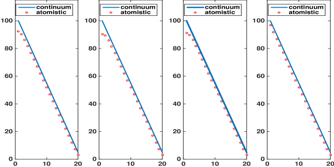
Figure 2. Testing several boundary conditions for the one-dimensional model. Left to right: A unit force applied to the first atom; A unit force applied to the second atoms; Forces applied to both atoms; Traction boundary condition that will be derived in the next section.

2.1. The derivation of the traction BC

To understand the traction BC, we start by embedding the semi-infinite atom chain into an infinite chain. We recall that $x_{i}=i$, $i\in\mathbb{Z}$ denotes the equilibrium positions. We take the view point that the BCs acting on the atom at $x_{0}$ should be determined by the interaction of the semi-infinite chain with the atoms on the left ($i<0$), whose degrees of freedom will be implicitly incorporated. In other words, the atoms $x_{i}$, $i\in\mathbb{Z}_{-}$ serves as an environment for the system we consider. We will hence distinguish the two groups of atoms by referring them as system atoms and environment atoms, respectively. This is based on our observation that most atomistic simulations are focused on part of the entire sample due to the small spatial scale associated with molecular models.

The problem now is reduced to removing the atoms in the environment. To facilitate the reduction of degrees of freedom from the whole chain to the semi-infinite, we will take the harmonic approximation. This amounts to assuming that the interaction between the atoms $x_{i}$ and $x_{j}$ is harmonic if either $i<0$ or $j<0$. In this paper, we focus our attention to static problems, which can be formulated as an energy minimization problem. For the current problem, the potential energy will be divided into several terms in accordance with the partition of the system,

(1) $$E=E_{\text{sys}}+E_{\text{int}}+E_{\text{env}}$$

where $E_{\text{sys}}$ is the interaction among the atoms in the semi-infinite chain on the right:

(2) $$E_{\text{sys}}=\sum_{i\geq 0}\bigl{(}V(y_{i+2}-y_{i})+V(y_{i+1}-y_{i})\bigr{)}.$$

Meanwhile $E_{\text{int}}$ collects the interaction terms between a system atom and an environmental atom. In terms of the displacement $u_{j}=y_{j}-x_{j}$, we have,

(3) $$E_{\text{int}}=\frac{\kappa_{1}}{2}(u_{0}-u_{-1})^{2}+\frac{\kappa_{2}}{2}(u_{0}-u_{-2})^{2}+\frac{\kappa_{2}}{2}(u_{1}-u_{-1})^{2},$$

where $\kappa_{1}=V^{\prime\prime}(1)$ and $\kappa_{2}=V^{\prime\prime}(2)$ are two stiffness constants for nearest-neighbor and next-nearest-neighbor interactions. Further, $E_{\text{env}}$ denotes the energy for the environment, given by

(4) $$E_{\text{env}}=\sum_{i<0}\bigl{[}\frac{\kappa_{1}}{2}(u_{i}-u_{i-1})^{2}+\frac{\kappa_{2}}{2}(u_{i}-u_{i-2})^{2}\bigr{]}.$$

Since the interaction is assumed to be next-nearest-neighbor, the environment atoms only interact with atoms with reference positions $x_{0}$ and $x_{1}$, but not other system atoms. Given the displacement $u_{0}$ and $u_{1}$, the force balance equations for the environment atoms can be written as

(5) $$\kappa_{2}(u_{j+2}-2u_{j}+u_{j-2})+\kappa_{1}(u_{j+1}-2u_{j}+u_{j-1})=0,\qquad j\in\mathbb{Z}_{-}.$$

The general solution of this finite difference equation is given by,

(6) $$u_{j}=A+Bj+C\lambda^{j}+D\lambda^{-j},$$

where $\lambda$ is a root of the characteristic polynomial associated to (5) (the other roots are $1/\lambda$ and $1$ with multiplicity $2$):

(7) $$\lambda=-1-\dfrac{\kappa_{1}}{2\kappa_{2}}\left[1-\sqrt{1+\frac{4\kappa_{2}}{\kappa_{1}}}\,\right].$$

We collect some elementary properties of $\lambda$ in the following lemma.

Lemma 1.

Assume $\kappa_{1}>0$ and $\kappa=\kappa_{1}+4\kappa_{2}>0$, we have $\lvert\lambda\rvert\leq 1$ and $-\kappa_{2}\lambda\geq 0$.

Proof.

First notice that

$$1+\frac{4\kappa_{2}}{\kappa_{1}}\leq 1+\frac{4\kappa_{2}}{\kappa_{1}}+\frac{4\kappa_{2}^{2}}{\kappa_{1}^{2}}=\Bigl{(}1+\frac{2\kappa_{2}}{\kappa_{1}}\Bigr{)}^{2},$$

which yields

$$1-\sqrt{1+\frac{4\kappa_{2}}{\kappa_{1}}}\geq-\frac{2\kappa_{2}}{\kappa_{1}}.$$

For $\kappa_{2}>0$, we then get

$$0\leq-\frac{\kappa_{1}}{2\kappa_{2}}\biggl{(}1-\sqrt{1+\frac{4\kappa_{2}}{\kappa_{1}}}\biggr{)}\leq 1.$$

Hence, by definition of $\lambda$ in (7), we get $\lambda\in[-1,0]$.

For $\kappa_{2}<0$, we have

$$-\frac{\kappa_{1}}{2\kappa_{2}}\biggl{(}1-\sqrt{1+\frac{4\kappa_{2}}{\kappa_{1}}}\biggr{)}\geq 1.$$

This yields $\lambda\geq 0$. Since $1+4\kappa_{2}/\kappa_{1}<1$, we also have

$$\sqrt{1+\frac{4\kappa_{2}}{\kappa_{1}}}\geq 1+\frac{4\kappa_{2}}{\kappa_{1}}$$

and hence

$$-\frac{\kappa_{1}}{2\kappa_{2}}\biggl{(}1-\sqrt{1+\frac{4\kappa_{2}}{\kappa_{1}}}\biggr{)}\leq-\frac{\kappa_{1}}{2\kappa_{2}}\biggl{(}1-1-\frac{4\kappa_{2}}{\kappa_{1}}\biggr{)}=2.$$

We conclude that $\lambda\leq 1$. ∎

Since $\lvert\lambda\rvert<1$, $\lambda^{j}$ grows exponentially as $j\to-\infty$ and hence unphysical. This leads to the requirement that $C=0$. The positions of the atoms at $x_{0}$ and $x_{1}$ further provide two BCs for (5). The remaining one degree of freedom is determined by the traction at the boundary,

(8) $$-\kappa_{1}(u_{0}-u_{-1})-\kappa_{2}(u_{0}-u_{-2})-\kappa_{2}(u_{1}-u_{-1})=T,$$

where $T$ is the prescribed traction at the boundary (scalar in $1D$). Intuitively, the traction across a material interface is given by the sum of the forces between two atoms that are on different sides of the interface [Admal2010unified, WuLi14]. This is indeed non-trivial, especially for multi-body interactions. But formulas are available for most empirical potentials [WuLi14].

Remark 2.

We further remark that the traction is conserved since no external force acts on the fictitious atoms: For $j\in\mathbb{Z}_{-}$,

$$\Bigl{(}-\kappa_{1}(u_{j}-u_{j-1})-\kappa_{2}(u_{j}-u_{j-2})\Bigr{)}-\kappa_{2}(u_{j+1}-u_{j-1})\\ \stackrel{{\scriptstyle\eqref{eq:fdhalfchain}}}{{=}}\Bigl{(}-\kappa_{1}(u_{j+1}-u_{j})-\kappa_{2}(u_{j+2}-u_{j})\Bigr{)}-\kappa_{2}(u_{j+1}-u_{j-1})\\ =-\kappa_{1}(u_{j+1}-u_{j})-\kappa_{2}(u_{j+1}-u_{j-1})-\kappa_{2}(u_{j+2}-u_{j}).$$

The solution to (5) can now be found. In particular, the coefficients are

$$A=\frac{-\lambda^{-1}u_{0}+u_{1}+T/\kappa}{1-\lambda^{-1}},\quad B=-T/\kappa,\quad\text{and}\quad C=\frac{u_{0}-u_{1}-T/\kappa}{1-\lambda^{-1}},$$

where $\kappa=\kappa_{1}+4\kappa_{2}$. As a result, the displacements $u_{-1}$ and $u_{-2}$ are given by

(9a) $$u_{-1}=(1+\lambda)u_{0}-\lambda u_{1}+(1-\lambda)T/\kappa;$$

(9b) $$u_{-2}=(1+\lambda)u_{-1}-\lambda u_{0}+(1-\lambda)T/\kappa.$$

Notice that $u_{-1}$ and $u_{-2}$ depend linearly on the displacements $u_{0}$, $u_{1}$ and the traction $T$. This is a result of the harmonic approximation in the environment. Now that the degrees of freedom associated with the atoms further on the left are removed, we can formulate the boundary value problem for the semi-infinite atom chain $x_{i}$, $i\in\mathbb{Z}_{+}\cup\{0\}$ in terms of ghost atoms $x_{-1}$ and $x_{-2}$ at the boundary. In general, the number of needed layers of atoms is determined by the interaction range.

With the BCs, the molecular statics model is complete. We consider a slightly more general problem by allowing body forces $f_{i}$ to be applied to the system atoms. In this case, the force balance equations read as follows,

(10a) $$-V^{\prime}(y_{j+2}-y_{j})-V^{\prime}(y_{j+1}-y_{j})+V^{\prime}(y_{j}-y_{j-1})+V^{\prime}(y_{j}-y_{j-2})=f_{j},\qquad j\geq 2$$

(10b) $$-V^{\prime}(y_{3}-y_{1})-V^{\prime}(y_{2}-y_{1})+V^{\prime}(y_{1}-y_{0})+\kappa_{2}(u_{1}-u_{-1})=f_{1},$$

(10c) $$-V^{\prime}(y_{2}-y_{0})-V^{\prime}(y_{1}-y_{0})+\kappa_{1}(u_{0}-u_{-1})+\kappa_{2}(u_{0}-u_{-2})=f_{0},$$

together with the BCs given by (9).

Another observation is that due to the semi-infinite nature, (10)-(9) can only determine $u$ up to a constant. To uniquely fix the arbitrary constant, we choose $u_{0}=0$. In addition, while the solution $u$ can be a linear function that corresponds to a uniformly stretched (or compressed) state, it is natural to exclude those solutions that grow superlinearly at infinity [luskin2013atomistic]. Hence, the complete set of BCs for the semi-infinite chain consists of the traction BC (9) and the conditions

(11a) $$u_{0}=0;$$

(11b) $$\limsup_{j\to\infty}\frac{\lvert u_{j}\rvert}{j}<\infty.$$

We emphasize that the above two BCs are associated with the semi-infinite chain under consideration, but not the traction at the left end of the chain. For finite system with a right boundary, appropriate BCs should be chosen to replace (11) according to the physical situation. Our emphasis, however, is on the traction condition at the left boundary.

Let us summarize the general framework for our BC construction in one-dimensional systems as follows

• Supplement the system with a fictitious environment of atoms with linear approximation;

• Solve the positions of the environmental atoms with the condition of fixed traction;

• The BC of the atomistic system is then given in terms of the positions of the ghost atoms.

This procedure can be clearly generalized to one-dimensional atomistic systems with arbitrary short-range interactions. The number of BCs depends on the interaction range.

Next, we turn to several properties of the BCs. These will help us better understand the traction BC and also facilitate the extension to higher dimension.

2.2. The continuum limit

For continuum elasticity models, traction BCs are imposed as the normal component of the stress. In this subsection, we show that the continuum limit of the reduced system (10), together with the BCs (9), leads to the Cauchy-Born elasticity with continuum traction BC in elasticity. Hence, our BCs (9) can be viewed as the molecular statics analog of the traction boundary condition in continuum elasticity.

To this end, we adopt the natural rescaling of the system such that the distance between nearest-neighbor atoms in equilibrium becomes $\varepsilon$. We will use superscript to make explicit the dependence on the scaling parameter $\varepsilon$. Hence, the equilibrium positions scale to $x_{j}^{\varepsilon}=j\varepsilon$, $j\in\mathbb{Z}_{+}\cup\{0\}$ and the deformed positions are $y_{j}^{\varepsilon}=x_{j}^{\varepsilon}+u^{\varepsilon}(x_{j}^{\varepsilon})$. We rewrite the force balance equation and the traction BC accordingly:

(12a) $$-V^{\prime}\Bigl{(}\frac{y_{j+2}^{\varepsilon}-y_{j}^{\varepsilon}}{\varepsilon}\Bigr{)}-V^{\prime}\Bigl{(}\frac{y_{j+1}^{\varepsilon}-y_{j}^{\varepsilon}}{\varepsilon}\Bigr{)}+V^{\prime}\Bigl{(}\frac{y_{j}^{\varepsilon}-y_{j-1}^{\varepsilon}}{\varepsilon}\Bigr{)}+V^{\prime}\Bigl{(}\frac{y_{j}^{\varepsilon}-y_{j-2}^{\varepsilon}}{\varepsilon}\Bigr{)}=\varepsilon f_{j},\qquad j\geq 2$$

(12b) $$-V^{\prime}\Bigl{(}\frac{y_{3}^{\varepsilon}-y_{1}^{\varepsilon}}{\varepsilon}\Bigr{)}-V^{\prime}\Bigl{(}\frac{y_{2}^{\varepsilon}-y_{1}^{\varepsilon}}{\varepsilon}\Bigr{)}+V^{\prime}\Bigl{(}\frac{y_{1}^{\varepsilon}-y_{0}^{\varepsilon}}{\varepsilon}\Bigr{)}+\kappa_{2}\Bigl{(}\frac{u_{1}^{\varepsilon}-u_{-1}^{\varepsilon}}{\varepsilon}\Bigr{)}=\varepsilon f_{1},$$

(12c) $$-V^{\prime}\Bigl{(}\frac{y_{2}^{\varepsilon}-y_{0}^{\varepsilon}}{\varepsilon}\Bigr{)}-V^{\prime}\Bigl{(}\frac{y_{1}^{\varepsilon}-y_{0}^{\varepsilon}}{\varepsilon}\Bigr{)}+\kappa_{1}\Bigl{(}\frac{u_{0}^{\varepsilon}-u_{-1}^{\varepsilon}}{\varepsilon}\Bigr{)}+\kappa_{2}\Bigl{(}\frac{u_{0}^{\varepsilon}-u_{-2}^{\varepsilon}}{\varepsilon}\Bigr{)}=\varepsilon f_{0}$$

with

(13a) $$u_{-1}^{\varepsilon}=(1+\lambda)u_{0}^{\varepsilon}-\lambda u_{1}^{\varepsilon}+\varepsilon(1-\lambda)T/\kappa;$$

(13b) $$u_{-2}^{\varepsilon}=(1+\lambda)u_{-1}^{\varepsilon}-\lambda u_{0}^{\varepsilon}+\varepsilon(1-\lambda)T/\kappa.$$

We now take the continuum limit $\varepsilon\to 0$. To the leading order, the equation (12a) becomes

(14) $$-\operatorname{div}\bigl{[}V^{\prime}(y^{\prime}(x))+2V^{\prime}(2y^{\prime}(x))\bigr{]}=f(x).$$

Note that for the current atomistic interaction potential, the Cauchy-Born stored energy density is given by [EMing:2007a]:

(15) $$W_{\mathrm{CB}}(A)=V\bigl{(}I+A\bigr{)}+V\bigl{(}2(I+A)\bigr{)}.$$

Hence, (14) is exactly the force balance equation for the Cauchy-Born elasticity since

(16) $$\partial_{A}W_{\mathrm{CB}}(u^{\prime})=V^{\prime}\bigl{(}1+u^{\prime}(x)\bigr{)}+2V^{\prime}\bigl{(}2+2u^{\prime}(x)\bigr{)}.$$

Combining (12b), (12c) and the BCs (13), we get

(17) $$-V^{\prime}\Bigl{(}\frac{y_{3}^{\varepsilon}-y_{1}^{\varepsilon}}{\varepsilon}\Bigr{)}-V^{\prime}\Bigl{(}\frac{y_{2}^{\varepsilon}-y_{1}^{\varepsilon}}{\varepsilon}\Bigr{)}-V^{\prime}\Bigl{(}\frac{y_{2}^{\varepsilon}-y_{0}^{\varepsilon}}{\varepsilon}\Bigr{)}=\varepsilon f_{1}+\varepsilon f_{0}+T.$$

To the leading order, this yields

(18) $$-V^{\prime}\bigl{(}1+u^{\prime}(0)\bigr{)}-2V^{\prime}\bigl{(}2+2u^{\prime}(0)\bigr{)}=T.$$

As the left hand side is equal to $n\cdot\partial_{A}W_{\mathrm{CB}}(u^{\prime})\big{|}_{x=0}$, where $n$ is the unit exterior normal, the BC (18) is exactly the traction BC for the elastic energy density $W_{\mathrm{CB}}$.

2.3. Linear stability at the equilibrium

We also make the observe that the force balance equations (12) with the traction BC (13) can be viewed as a finite difference system with BCs. It is then natural to analyze the stability of such a finite difference system, similar in spirit to the analysis in the context of atomistic-to-continuum methods [LuMing:13, LuMing:14]. We also note that the stability is the crucial ingredient for the rigorous proof of the continuum limit in §2.2. The stability of molecular statics models under periodic and Dirichlet BCs have been analyzed in [EMing:2007a, ehrlacher2013analysis].

To understand the stability, we linearize the force balance equations (10) at the equilibrium (undeformed) state, yielding,

(19) $$-\kappa_{2}(u_{j+2}-2u_{j}+u_{j-2})-\kappa_{1}(u_{j+1}-2u_{j}+u_{j-1})=f_{j},\qquad j\geq 0,$$

supplemented by the BC (9) and (11). Given $T$, we define the map $H_{T}:l^{2}(\mathbb{N})\to l^{2}(\mathbb{N})$ as

(20) $$(H_{T}u)_{j}=-\kappa_{2}(u_{j+2}-2u_{j}+u_{j-2})-\kappa_{1}(u_{j+1}-2u_{j}+u_{j-1}),\qquad j\geq 0$$

with $u_{-1}$ and $u_{-2}$ determined by (13) (and hence the dependence on $T$). Thus we have

(21) $$H_{T}(u)_{j}-H_{0}(u)_{j}=\begin{cases}-\bigl{(}\kappa_{2}(2+\lambda)+\kappa_{1}\bigr{)}(1-\lambda)T/\kappa,&j=0;\\ -\kappa_{2}(1-\lambda)T/\kappa,&j=1;\\ 0,&\text{otherwise}.\end{cases}$$

Let us introduce a few short-hand notations. First we define the forward difference as

(22) $$(Du)_{j}=u_{j+1}-u_{j}.$$

Moreover, the discrete Laplacian is given by

(23) $$(\Delta_{d}u)_{j}=u_{j+1}-2u_{j}+u_{j-1}.$$

Direct calculations yield,

(24) $$(\Delta_{d}\Delta_{d}u)_{j}+4(\Delta_{d}u)_{j}=\bigl{(}u_{j+2}-4u_{j+1}+6u_{j}-4u_{j-1}+u_{j-2}\bigr{)}+4\bigl{(}u_{j+1}-2u_{j}+u_{j-1}\bigr{)}\\ =(u_{j+2}-2u_{j}+u_{j-2}).$$

With these preparations, we calculate the quadratic form $\left\langle u,H_{0}(u)\right\rangle$:

(25) $$\left\langle u,H_{0}u\right\rangle =-\kappa_{2}\sum_{j=0}^{\infty}u_{j}\bigl{(}(\Delta_{d}\Delta_{d}u)_{j}+4(\Delta_{d}u)_{j}\bigr{)}-\kappa_{1}\sum_{j=0}^{\infty}u_{j}(\Delta u)_{j}$$

$$=-\kappa_{2}\sum_{j=0}^{\infty}u_{j}(\Delta\Delta u)_{j}-\kappa\sum_{j=0}^{\infty}u_{j}(\Delta u)_{j}$$

Summation by parts gives (recall that $u_{0}=0$)

(26) $$\sum_{j=0}^{\infty}u_{j}(\Delta u)_{j}=-\sum_{j=0}^{\infty}\lvert(Du)_{j}\rvert^{2}.$$

For the fourth order term, we get

(27) $$\sum_{j=0}^{\infty}u_{j}(\Delta\Delta u)_{j}=\sum_{j=0}^{\infty}\lvert(\Delta u)_{j}\rvert^{2}-u_{-1}(u_{1}+u_{-1})=\sum_{j=0}^{\infty}\lvert(\Delta u)_{j}\rvert^{2}+\lambda(1-\lambda)u_{1}^{2},$$

where in the last equality, we used $u_{-1}=-\lambda u_{1}$ in the case $T=0$ and $u_{0}=0$.

Finally, we have,

(28) $$\left\langle u,H_{0}u\right\rangle=\kappa\sum_{j=0}^{\infty}\lvert(Du)_{j}\rvert^{2}-\kappa_{2}\sum_{j=0}^{\infty}\lvert(\Delta u)_{j}\rvert^{2}-\kappa_{2}\lambda(1-\lambda)u_{1}^{2}.$$

By Lemma 1, we have $-\kappa_{2}\lambda(1-\lambda)>0$ as long as $\kappa_{1}>0$ and $\kappa>0$. Thus, we have

(29) $$\left\langle u,H_{0}u\right\rangle\geq\kappa\sum_{j=0}^{\infty}\lvert(Du)_{j}\rvert^{2}-\kappa_{2}\sum_{j=0}^{\infty}\lvert(\Delta u)_{j}\rvert^{2}$$

Therefore, the scheme is stable as long as the underlying atomistic model is stable.

For a general traction $T$, we have

(30) $$\left\langle u,H_{T}u\right\rangle=\left\langle u,H_{0}u\right\rangle-\frac{\kappa_{2}}{\kappa}(1-\lambda)Tu_{1}.$$

Therefore, the stability follows from the stability in the case of $T=0$.

Remark 3.

This analysis also shows that if $\lambda$ in (9) is replaced by an appropriate approximation, i.e., $\widetilde{\lambda}\approx\lambda$ satisfying $-\kappa_{2}\widetilde{\lambda}(1-\widetilde{\lambda})>0$, a stable model would also be obtained.

We show that a careless choice of the BC may lead to instability of the scheme. Instead of (9), let us consider an alternative set of BCs (to distinguish, we use $\widetilde{u}$ for the displacement)

(31a) $$\widetilde{u}_{-1}=(1+\lambda^{-1})\widetilde{u}_{0}-\lambda^{-1}\widetilde{u}_{1}+(\lambda^{-1}-1)T/\kappa;$$

(31b) $$\widetilde{u}_{-2}=(1+\lambda^{-1})\widetilde{u}_{-1}-\lambda^{-1}\widetilde{u}_{0}+(\lambda^{-1}-1)T/\kappa.$$

It is straightforward to check that this set of BC also yields traction $T$ at the boundary

(32) $$-\kappa_{1}(\widetilde{u}_{0}-\widetilde{u}_{-1})-\kappa_{2}(\widetilde{u}_{0}-\widetilde{u}_{-2})-\kappa_{2}(\widetilde{u}_{1}-\widetilde{u}_{-1})=T,$$

and hence consistent with the traction BC in continuum elasticity. However, the resulting scheme with the BC (31) is not stable. In fact, we even lose uniqueness: it is easy to check that $\widetilde{u}_{j}=\lambda^{j}-1$ for $j\geq-2$ satisfies

(33) $$-\kappa_{2}(\widetilde{u}_{j+2}-2\widetilde{u}_{j}+\widetilde{u}_{j-2})-\kappa_{1}(\widetilde{u}_{j+1}-2\widetilde{u}_{j}+\widetilde{u}_{j-1})=0,\qquad j\geq 0,$$

and also at the boundary

(34) $$\widetilde{u}_{-1}=(1+\lambda^{-1})\widetilde{u}_{0}-\lambda^{-1}\widetilde{u}_{1};$$

(35) $$\widetilde{u}_{-2}=(1+\lambda^{-1})\widetilde{u}_{-1}-\lambda^{-1}\widetilde{u}_{0};$$

(36) $$\widetilde{u}_{0}=0;$$

(37) $$\limsup_{j\to\infty}\frac{\lvert\widetilde{u}_{j}\rvert}{j}=0.$$

2.4. Connection to BCs with applied forces at the boundary

As we alluded to at the beginning of this section, it is also possible to apply forces ($T_{0}$ and $T_{1}$) directly at the boundary to create a traction. But it is not immediately clear how much forces to apply on each of the two atoms at the boundary. Here we will demonstrate the connection to that approach. In particular, this discussion will also shed light on the selection of the forces.

If we substitute (9) into the force balance equation (10), we get

$$-V^{\prime}(y_{3}-y_{1})-V^{\prime}(y_{2}-y_{1})+V^{\prime}(y_{1}-y_{0}) =f_{1}+T_{1};$$

$$-V^{\prime}(y_{2}-y_{0})-V^{\prime}(y_{1}-y_{0})=f_{0}+T_{0}.$$

with

(38) $$T_{1} =\kappa_{2}(u_{-1}-u_{0})=\kappa_{2}\bigl{(}(1+\lambda)(u_{0}-u_{1})+(1-\lambda)T/\kappa\bigr{)};$$

(39) $$T_{0} =\kappa_{2}(u_{-2}-u_{0})+\kappa_{1}(u_{-1}-u_{0})$$

$$=\lambda\bigl{(}\kappa_{1}+\kappa_{2}(1+\lambda)\bigr{)}(u_{0}-u_{1})+(1-\lambda)\bigl{(}\kappa_{1}+\kappa_{2}(2+\lambda)\bigr{)}T/\kappa.$$

This provides the formulas for the forces. An important observation, however, is that these forces should depend on the displacement of the atoms at $x_{0}$ and $x_{1}$.

2.5. Traction BC from the Green’s function

To facilitate the extension of the BC to two dimensional systems, we take yet another point of view of the traction BC, from the lattice Green’s function perspective.

Let us define the lattice Green’s function associated with the model (5),

(40) $$-\kappa_{2}(G_{j+2}-2G_{j}+G_{j-2})-\kappa_{1}(G_{j+1}-2G_{j}+G_{j-1})=\delta(j),\qquad j\in\mathbb{Z}.$$

In general, the lattice Green’s functions are useful analytical tools for studying lattice distortions around defects (see e.g., [Tewary1973]). A typical route to compute the Green’s function is via a Fourier transform,

(41) $$\widehat{G}(\xi)=\sum_{j\in\mathbb{Z}}e^{i\xi j}G_{j},\qquad\xi\in[-\pi,\pi)$$

with the inverse given by,

(42) $$G_{j}=\frac{1}{2\pi}\int_{-\pi}^{\pi}e^{-i\xi j}\widehat{G}(\xi)\,\mathrm{d}\xi$$

This leads to

(43) $$-\kappa_{2}\bigl{(}e^{2i\xi}-2+e^{-2i\xi}\bigr{)}\widehat{G}(\xi)-\kappa_{1}\bigl{(}e^{i\xi}-2+e^{-i\xi}\bigr{)}\widehat{G}(\xi)=1,$$

and

(44) $$\widehat{G}(\xi)=\frac{1}{4\kappa_{2}\sin^{2}(\xi)+4\kappa_{1}\sin^{2}(\xi/2)}.$$

However, due to the singularity at $\xi=0$, the integral (42) with $\widehat{G}$ given above is not well defined. A remedy [MaRo02] is to modify (42):

(45) $$G_{j} =\frac{1}{2\pi}\int_{-\pi}^{\pi}\frac{e^{-i\xi j}-1}{4\kappa_{2}\sin^{2}(\xi)+4\kappa_{1}\sin^{2}(\xi/2)}\,\mathrm{d}\xi$$

$$=-\frac{1}{2\pi}\int_{-\pi}^{\pi}\frac{2\sin^{2}(\xi j/2)}{4\kappa_{2}\sin^{2}(\xi)+4\kappa_{1}\sin^{2}(\xi/2)}\,\mathrm{d}\xi.$$

Conceptually, the Green’s function (40) is only defined up to a constant, and one can fix $G_{0}=0$ by subtracting a (infinite) constant from (42).

As a result, the integral is now well defined as the integrand is regular as $\xi\to 0$. The function $G_{j}$ defined this way still satisfies the equations (40). We now make the connections to the BCs (9).

Lemma 2.

For $j\leq 0$,

(46) $$G_{j-1}=(1+\lambda)G_{j}-\lambda G_{j+1}$$

Proof.

Rewrite (45) using a change of variable $z=\exp(i\xi)$ and the characteristic polynomial associated to the denominator, we get

$$G_{j} =\frac{1}{2\pi\kappa_{2}i}\int_{\lvert z\rvert=1}\frac{(z^{-j}-1)z}{(z-1)^{2}(z-\lambda)(z-\lambda^{-1})}\,\mathrm{d}z$$

$$=\frac{1}{2\pi\kappa_{2}i}\lim_{\epsilon\to 0}\int_{\gamma_{\epsilon}}\frac{(z^{-j}-1)z}{(z-1)^{2}(z-\lambda)(z-\lambda^{-1})}\,\mathrm{d}z$$

where the contour $\gamma_{\epsilon}$ is given by the boundary of $B_{1}(0)\backslash B_{\epsilon}(1)$ on the complex plane. The second equality uses the fact that the integrand is regular as $z\to 1$.

Using this representation, we have

$$G_{j-1}-(1+\lambda)G_{j}+\lambda G_{j+1} =\frac{1}{2\pi\kappa_{2}i}\lim_{\epsilon\to 0}\int_{\gamma_{\epsilon}}\frac{z^{-j}\bigl{(}z^{2}-(1+\lambda)z+\lambda\bigr{)}}{(z-1)^{2}(z-\lambda)(z-\lambda^{-1})}\,\mathrm{d}z$$

$$=\frac{1}{2\pi\kappa_{2}i}\lim_{\epsilon\to 0}\int_{\gamma_{\epsilon}}\frac{z^{-j}}{(z-1)(z-\lambda^{-1})}\,\mathrm{d}z.$$

As $j\leq 0$ and $\lvert\lambda\rvert<1$, the integrand is holomorphic in $B_{1}(0)\backslash B_{\epsilon}(1)$ for any $\epsilon$, and hence the integral vanishes for any $\epsilon$ by Cauchy’s integral theorem. Therefore, (46) holds. ∎

The equation (46) is exactly in the same form as the BCs (9) when $T=0$. This is not surprising, since the Green’s function represents a special set of solutions. In particular, $G_{j}$ satisfies the homogeneous difference equations (5). Nevertheless, this simple observation can be employed to determine the coefficients in the BCs by using the Green’s functions as test functions. This will be implemented for problems in two-dimensions, and the implementation will be discussed in the next sections.

3. Implementation in two-dimensional models

Here we demonstrate how the BC can be extended to two-dimensional systems.

3.1. The traction BC and the induced boundary value problem

For multi-dimensional problems, the BC is typically non-local [MeKaLi06], in that the displacement of all the atoms at the boundary is coupled. It is also possible to consider nonlocal boundary conditions, for example, in the spirit of the boundary element method for molecular static models by one of the authors [Li:12]. Another alternative is to seek a local BC, in the sense that the position of the ghost atoms are only determined by the positions of nearby atoms in the system. To make the dependence local, we would employ a “local flattening” of the boundary. Roughly speaking, for an atom at the boundary, the position is determined by a homogeneous approximation of the local atom configuration with the local value of the traction tensor.

To better explain the idea, we consider the face-centered cubic (FCC) lattice of Aluminum with the axis aligned in $\langle 110\rangle$, $\langle 001\rangle$ and $\langle 1\bar{1}0\rangle$ orientations. When projected to the $\langle 1\bar{1}0\rangle$ plane, the lattice spacing in the horizontal and vertical directions are $\frac{a_{0}}{\sqrt{2}}$ and $\frac{a_{0}}{2}$, respectively, which makes it look like a triangular lattice, as shown in Fig. 3. Again, we introduce ghost atoms outside the boundary in order to achieve the desired traction condition. They are represented by open circles in Fig. 3.

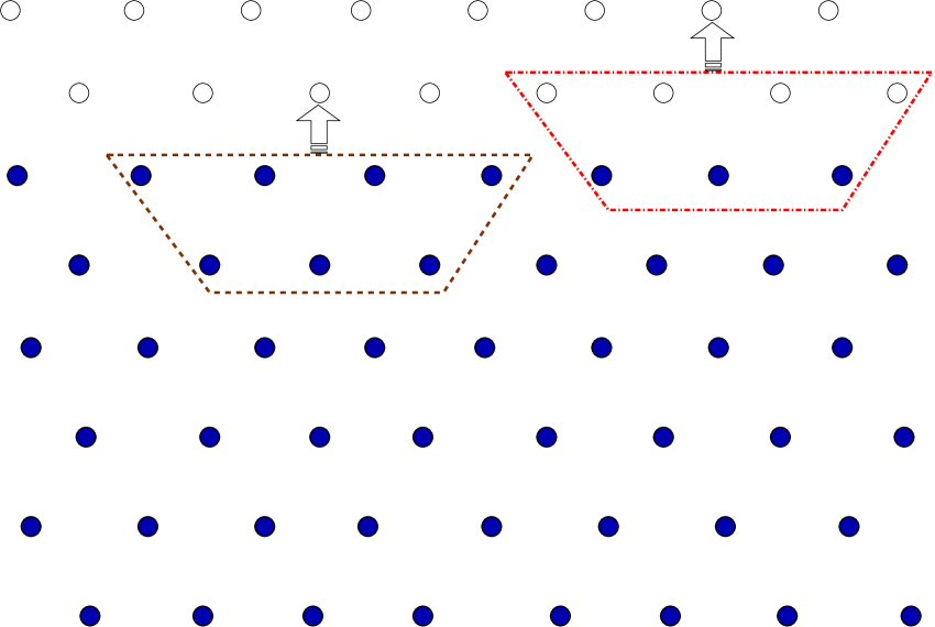
Figure 3. The projected atomic position of a FCC lattice. Filled circles: Atoms in the interior; Open circles: the ghost atoms introduced outside the boundary. The boxes contain the set of atoms $S_{j}$ that will be used to determine the displacement of the $j$th atom (see equation (47)).

Our main goal is to determine the actual position of the ghost atoms based on the displacement of the atoms in the interior and the applied traction $T$, which is a two-dimensional vector. In this case, it is in general cumbersome to obtain the exact boundary condition. Motivated by the one-dimensional traction BC, we seek an approximate BC in the following form,

(47) $$u_{j}=\sum_{i\in S_{j}}B_{ji}u_{i}+p_{j}.$$

The shift vector $p$ is similar to the non-homogeneous term in (9), and it will be determined so that the correct traction is obtained. In the case when $p=0$, this boundary condition would coincide with the BCs that models an environment that is at a mechanical equilibrium with zero stress [Li2009b, MeKaLi06]. In principle, an exact BC in this form can be derived, e.g., in [MeKaLi06], which mathematically, is a discrete analogue of the Dirichlet-to-Neumann (DtN) map. The exact expression is typically nonlocal, in that the summation is over all the atoms near the boundary. But here we choose a local approximation, and restrict the summation in (47) to those atoms that are close to the $j$ atoms. These neighbors are collected by the set $S_{j}.$ Due to the translational symmetry of the lattice, we will use the same set of neighbors when implementing the formula (47), which is also demonstrated in Fig. 3. More specifically, we start with the layer of ghost atoms closest to the boundary and apply the BCs (47). Once the displacement of these atoms are updated, we move to the next layer, and these steps will be repeated until the position of all the ghost atoms are updated.

We now discuss how to determine the coefficients $B_{ji}$. Since they are independent of the applied traction, they can be computed for the case $T=0$ and $p=0.$ In this case, these coefficients can be determined using an optimization procedure, developed in [Li2009b]. More specifically, we choose an objective function as follows,

(48) $$\min h,\quad h=\sum_{k}|G_{j,k}-\sum_{i}B_{ji}G_{i,k}|^{2}.$$

Here $G_{j,k}$ is the two-dimensional lattice Green’s function [Tewary1973]. The main observation is that the BC should by satisfied by special solutions, especially the lattice Green’s functions $G_{i,k}$, which corresponds to the solution of the linearized molecular statics model when a point force is applied on the $k$th atom. This was already observed for the one-dimensional model. Ideally, the objective function would be zero when the BC is exact. Further, we introduce a constraint,

(49) $$\sum_{i}B_{ji}=I,$$

so that the constant solutions are admitted. This is also seen in the one-dimensional system: The two coefficients in (9) add up to 1.

It remains to estimate the vector $p$. In principle, it should be determined by requiring the traction to arrive at a prescribed value. The total tractions along the boundary is given by the sum of the forces [Admal2010unified, WuLi14],

(50) $$t=\sum_{i\in\Omega,j\notin\Omega}f_{ij}.$$

Here, $f_{ij}$ comes from a force decomposition. Namely,

(51) $$f_{i}=\sum_{j\neq i}f_{ij},\quad f_{ij}=-f_{ji}.$$

This formula, which was already indicated by (8), is consistent with the intuition of Cauchy. The explicit expressions for the force decomposition (51), especially for multi-body potentials, can be found in [Chen2006local, WuLi14].

To control the local traction, we divide the region with ghost atoms into blocks, each denoted by $\Omega^{c}_{\alpha},$ $\alpha=1,2,\cdots,M$. The computational domain is denoted by $\Omega,$ and the intersection with $\Omega^{c}_{\alpha}$, is written as $\partial\Omega_{\alpha}.$ For each block $\Omega^{c}_{\alpha},$ we introduce a shift vector $p_{\alpha}$. They are chosen so that the traction along $\partial\Omega_{\alpha}$ agrees with a prescribed value $t_{\alpha}$. This arrangement is illustrated in Fig. 4.

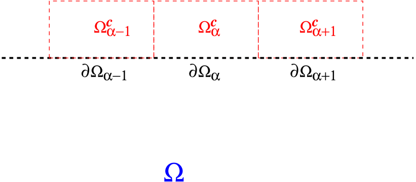
Figure 4. Imposing tractions along the boundary: $\Omega$ indicate the computational domain. The atoms outside the boundary are grouped into blocks $\Omega_{\alpha}^{c}$ with the intersection with the boundary given by $\partial\Omega_{\alpha}$. The traction on each $\partial\Omega_{\alpha}$ is prescribed.

We now put the mathematical models together.

(52) $$\left\{\begin{aligned} &\frac{\partial}{\partial u_{i}}V=0,&&\forall x_{i}\in\Omega,\\ &u_{j}=\sum_{i}B_{ji}u_{i}+p_{\alpha},&&\forall x_{j}\in\partial\Omega_{\alpha},\\ &\sum_{i\in\Omega,j\in\Omega_{\alpha}^{c}}f_{ij}=t_{\alpha}.&\end{aligned}\right.$$

The first set of equations represent the force balance in the interior, with potential energy given by $V$. The remaining equations serve as BCs with prescribed tractions $t_{\alpha}$. The unknowns are the atomic displacement, together with the shift vectors $p_{\alpha}$. The atomic degrees of freedom associated with the atoms outside $\Omega$ has been implicitly taken into account by the second and third equations in (52). In the next section, we will discuss an implementation method.

3.2. Numerical implementations

Our reduced model (52) consists of a set of nonlinear algebraic equations. It is therefore natural to make use of iterative methods, such as the quasi-Newton’s method. In general, this requires the approximation of the Jacobian matrix, since the analytical form is usually not available. The convergence is typically slow, especially when the system is not well prepared.

To find an alternative, we notice that in the domain $\Omega$, the molecular statics model is associated with an energy. Therefore, for Dirichlet BCs, where the atoms outside the boundary are held fixed, the solution to the molecular statics model correspond to an energy minimization, which is usually more robust and much more efficient than solving the nonlinear equations.

We implement the equations by a domain decomposition approach, and alternate among the three sets of equations in (52). As an example to explain the idea, we may consider the coupling of the first two sets of equations and assume that $p_{\alpha}$ is given. We create a few overlapping layers, in which the atoms serve as both ghost atoms and interior atoms. This is illustrated by Fig. 5. In each iteration, we first update the displacement of all the ghost atoms including those in the overlapping region using (47) (or the second equation in (52)). We then turn to the interior atoms, assuming that other atoms are held fixed (open circles in Fig. 5). By minimizing the energy, we obtain the updated position of the interior atoms. The numerical implementation has been done with the BFGS package [Liu1989lbfgs]. This iteration can be continued until convergence is reached. This is simply the Schwartz iteration [toselli2005domain]) between the two models.

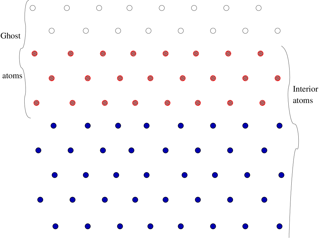
Figure 5. An overlapping domain decomposition.

3.3. Results from numerical experiments

As a test problem, we consider a dislocation dipole under a shear load. The atoms around the two dislocations with opposite Burgers vectors are shown in Fig. 6. The embedded atom model (EAM) [ercolessi1994interatomic] has been used as the interatomic potential.

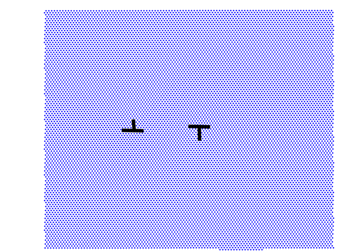
Figure 6. The atoms near the two dislocations.

We first manually control the vector $p=(p_{1},0),$ and observe the influence on the traction changes. As a quasi-static loading, we increase $p_{1}$ with small increment and then solve the molecular statics model using the domain decomposition method described in the previous section. For each step, we also compute the traction at the boundary. The history of the total boundary traction is shown in Fig. 7. We observe that the traction increases as $p_{1}$ increases. However, when $p_{1}$ reaches certain critical value, a sudden drop is observed. In this case, the two dislocations move to the boundary, and the entire sample undergoes a complete slip. Fig. 8 shows the atomic positions before and after the slip.

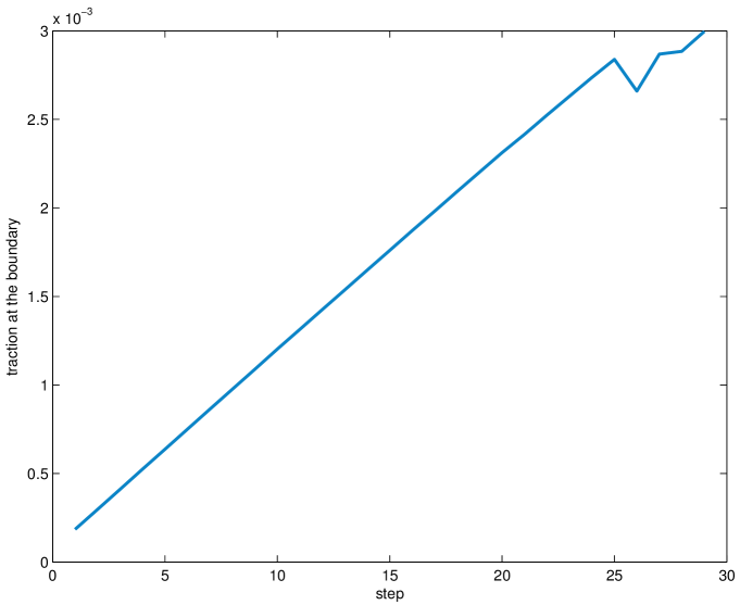
Figure 7. The history of the traction at the boundary.

Figure 8. The position of the atoms before and after the yield stress.

In the next experiment, we apply a uniform traction along the upper and lower boundaries. In Fig. 9, we show the resulting values of $p_{1}$ along the boundary. While, the resulting tractions have reached the prescribed values $(2\times 10^{-4},0)$, it is clear that the values for $p$ are not homogeneous, mainly due to the presence of the dislocations. The displacement is shown in Fig. 10, together with a close-up view of the atomic positions. All these results suggest that the atomic positions are not uniform. Compared to the simulations of dislocation dipoles using the Parrinello-Rahman method (e.g.,[wang2004calculating]), the current approach does not introduce periodic images of the dislocation dipole. Moreover, the uniform shear stress can be applied without forcing a uniform deformation along the boundaries.

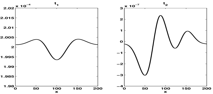
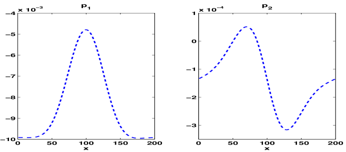
Figure 9. The traction (top) and the shift vector $p_{1}$ (bottom) along the upper boundary.

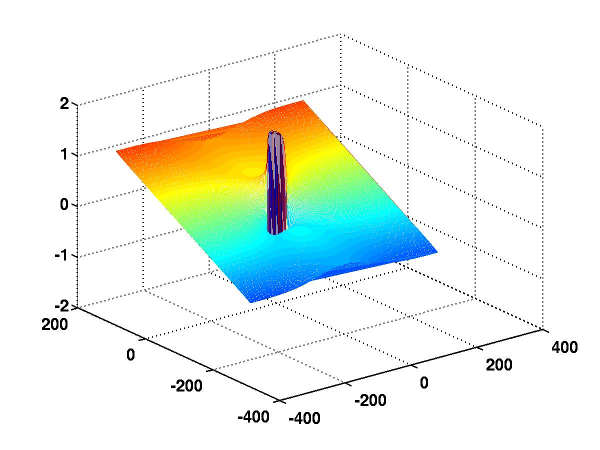
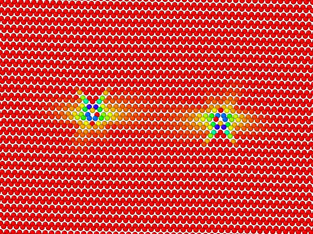
Figure 10. The displacement $u_{1}$ and a close-up view of the atoms near the two dislocations (generated in Ovito [stukowski2010visualization]).

4. Summary and Discussion

We have formulated boundary conditions that impose a traction force on a molecular statics model. These boundary conditions are derived by taking into account the surrounding elastic environment. Hence, the computational domain is part of a much bigger sample, and artificial boundary effects can be eliminated. In the continuum limit, these boundary conditions coincide with the Neumann boundary condition for continuum elasticity models. We have restricted our discussions to static problems. Extension to dynamic problems will be considered in future works.

Acknowledgment. The work of J.L. was supported in part by the Alfred P. Sloan foundation and National Science Foundation under award DMS-1312659.