Online Matrix Completion and Online Robust PCA

Abstract

This work studies two interrelated problems - online robust PCA (RPCA) and online low-rank matrix completion (MC). In recent work by Candès et al., RPCA has been defined as a problem of separating a low-rank matrix (true data), $L:=[\ell_{1},\ell_{2},\dots\ell_{t},\dots,\ell_{t_{\max}}]$ and a sparse matrix (outliers), $S:=[x_{1},x_{2},\dots x_{t},\dots,x_{t_{\max}}]$ from their sum, $M:=L+S$. Our work uses this definition of RPCA. An important application where both these problems occur is in video analytics in trying to separate sparse foregrounds (e.g., moving objects) and slowly changing backgrounds.

While there has been a large amount of recent work on both developing and analyzing batch RPCA and batch MC algorithms, the online problem is largely open. In this work, we develop a practical modification of our recently proposed algorithm to solve both the online RPCA and online MC problems. The main contribution of this work is that we obtain correctness results for the proposed algorithms under mild assumptions. The assumptions that we need are: (a) a good estimate of the initial subspace is available (easy to obtain using a short sequence of background-only frames in video surveillance); (b) the $\ell_{t}$’s obey a ‘slow subspace change’ assumption; (c) the basis vectors for the subspace from which $\ell_{t}$ is generated are dense (non-sparse); (d) the support of $x_{t}$ changes by at least a certain amount at least every so often; and (e) algorithm parameters are appropriately set.

I Introduction

Principal Components Analysis (PCA) is a tool that is frequently used for dimension reduction. Given a matrix of data $\bm{D}$, PCA computes a small number of orthogonal directions, called principal components, that contain most of the variability of the data. For relatively noise-free data that lies close to a low-dimensional subspace, PCA is easily accomplished via singular value decomposition (SVD). The problem of PCA in the presence of outliers is referred to as robust PCA (RPCA). In recent work, Candès et al. [2] posed RPCA as a problem of separating a low-rank matrix, $\bm{L}$, and a sparse matrix, $\bm{S}$, from their sum, $\bm{M}:=\bm{L}+\bm{S}$. They proposed a convex program called principal components’ pursuit (PCP) that provided a provably correct batch solution to this problem under mild assumptions. PCP solves

$$\min_{\tilde{\bm{L}},\tilde{\bm{S}}}\|\tilde{\bm{L}}\|_{*}+\lambda\|\tilde{\bm{S}}\|_{\operatorname{sum}}\quad\text{subject to}\quad\tilde{\bm{L}}+\tilde{\bm{S}}=\bm{M},$$

where $\|\cdot\|_{*}$ is the nuclear norm (sum of singular values), $\|\cdot\|_{\operatorname{sum}}$ is the sum of the absolute values of the entries, and $\lambda$ is an appropriately chosen scalar. The same program was analyzed in parallel by Chandrasekharan et al. [3] and later by Hsu et al. [4]. Since these works, there has been a large amount of work on batch approaches for RPCA and their performance guarantees.

When RPCA needs to be solved in a recursive fashion for sequentially arriving data vectors it is referred to as online (or recursive) RPCA. Online RPCA assumes that a short sequence of outlier-free (sparse component free) data vectors is available. An example application where this problem occurs is the problem of separating a video sequence into foreground and background layers (video layering) on-the-fly [2]. Video layering is a key first step for automatic video surveillance and many other streaming video analytics tasks. In videos, the foreground usually consists of one or more moving persons or objects and hence is a sparse image. The background images usually change only gradually over time [2], e.g., moving lake waters or moving trees in a forest, and hence are well modeled as lying in a low-dimensional subspace that is fixed or slowly changing. Also, the changes are global (dense) [2]. In most video applications, it is valid to assume that an initial short sequence of background-only frames is available and this can be used to estimate the initial subspace via SVD.

Often in video applications the sparse foreground $\bm{x}_{t}$ is actually the signal of interest, and the background $\bm{\ell}_{t}$ is the noise. In this case, the problem can be interpreted as one of recursive sparse recovery in (potentially) large but structured noise. Our result allows for $\bm{\ell}_{t}$ to be large in magnitude as long as it is structured. The structure we impose is that the $\bm{\ell}_{t}$’s lie in a low dimensional subspace that changes slowly over time.

In some other applications, instead of there being outliers, parts of a data vector may be missing entirely. When the (unknown) complete data vector is a column of a low-rank matrix, the problem of recovering it is referred to as matrix completion (MC). For example, recovering video sequences and tracking their subspace changes in the presence of easily detectable foreground occlusions. If the occluding object’s intensity is known and is significantly different from that of the background, its support can be obtained by simple thresholding. The background video recovery problem then becomes an MC problem. A nuclear norm minimization (NNM) based solution for MC was introduced in [5] and studied in [6]. The convex program here is to minimize the nuclear norm of $\tilde{\bm{M}}$ subject to $\tilde{\bm{M}}$ and $\bm{M}$ agreeing on all observed entries. Since then there has been a large amount of work on batch methods for MC and their correctness results.

I-A Problem Definition

Consider the online MC problem. Let $\mathcal{T}_{t}$ denote the set of missing entries at time $t$. We observe a vector $\bm{m}_{t}\in\mathbb{R}^{n}$ that satisfies

$$\bm{m}_{t}=\bm{I}_{\overline{\mathcal{T}}_{t}}{\bm{I}_{\overline{\mathcal{T}}_{t}}}^{\prime}\bm{\ell}_{t}\qquad\text{ for }t=t_{\mathrm{train}}+1,t_{\mathrm{train}}+2,\dots,t_{\max}.$$ (1)

with the possibility that $t_{\max}$ can be infinity too. Here $\bm{\ell}_{t}$ is such that, for $t$ large enough (quantified in Model 2.2), the matrix $\bm{L}_{t}:=[\bm{\ell}_{1},\bm{\ell}_{2},\dots,\bm{\ell}_{t}]$ is a low-rank matrix. Notice that by defining $\bm{m}_{t}$ as above, we are setting to zero the entries that are missed (see the notation section on page I-D).

Consider the online RPCA problem. At time $t$ we observe a vector $\bm{m}_{t}\in\mathbb{R}^{n}$ that satisfies

$$\bm{m}_{t}=\bm{\ell}_{t}+\bm{x}_{t}\qquad\text{ for }t=t_{\mathrm{train}}+1,t_{\mathrm{train}}+2,\dots,t_{\max}.$$ (2)

Here $\bm{\ell}_{t}$ is as defined above and $\bm{x}_{t}$ is the sparse (outlier) vector. We use $\mathcal{T}_{t}$ to denote the support set of $\bm{x}_{t}$.

For both problems above, for $t=1,2,\dots,t_{\mathrm{train}}$, we are given complete outlier-free measurements $\bm{m}_{t}=\bm{\ell}_{t}$ so that it is possible to estimate the initial subspace. For the video surveillance application, this would correspond to having a short initial sequence of background only images, which can often be obtained. For $t>t_{\mathrm{train}}$, the goal is to estimate $\bm{\ell}_{t}$ (or $\bm{\ell}_{t}$ and $\bm{x}_{t}$ in case of RPCA) as soon as $\bm{m}_{t}$ arrives and to periodically update the estimate of $\operatorname{range}(\bm{L}_{t})$.

In the rest of the paper, we refer to $\mathcal{T}_{t}$ as the missing/corrupted entries’ set.

I-B Related Work

Some other work that also studies the online MC problem (defined differently from above) includes [7, 8, 9, 10]. We discuss the connection with the idea from [7] in Section IV. The algorithm from [8], GROUSE, is a first order stochastic gradient method; a result for its convergence to the local minimum of the cost function it optimizes is obtained in [10]. The algorithm of [9], PETRELS, is a second order stochastic gradient method. It is shown in [9] that PETRELS converges to the stationary point of the cost function it optimizes. The advantage of PETRELS and GROUSE is that they do not need initial subspace knowledge. Another somewhat related work is [11].

Partial results have been provided for ReProCS for online RPCA in our older work [12]. In other more recent work [13] another partial result is obtained for online RPCA defined differently from above. Neither of these is a correctness result. Both require an assumption that depends on intermediate algorithm estimates. Another somewhat related work is [14] on online PCA with contaminated data. This does not model the outlier as a sparse vector but defines anything that is far from the data subspace as an outlier.

Some other works only provide an algorithm without proving any performance results, e.g., [15].

We discuss the most related works in detail in Sec III-C.

I-C Contributions

In this work we develop and study a practical modification of the Recursive Projected Compressive Sensing (ReProCS) algorithm introduced and studied in our earlier work [12] for online RPCA. We also develop a special case of it that solves the online MC problem. The main contribution of this work is that we obtain a complete correctness result for ReProCS-based algorithms for both online MC and online RPCA (or more generally, online sparse plus low-rank matrix recovery). Online algorithms are useful because they are causal (needed for applications like video surveillance) and, in most cases, are faster and need less storage compared to most batch techniques (we should mention here that there is some recent work on faster batch techniques as well, e.g., [16]). To the best of our knowledge, this work and an earlier conference version of this [1] may be among the first correctness results for online RPCA. The algorithm studied in [1] is more restrictive.

Moreover, as we will see, by exploiting temporal dependencies, such as slow subspace change, and initial subspace knowledge, our result is able to allow for a more correlated set of missing/corrupted entries than do the various results for PCP [2, 3, 4] or NNM [6] (see Sec. III).

Our result uses the overall proof approach introduced in our earlier work [12] that provided a partial result for online RPCA. The most important new insight needed to get a complete result is described in Section IV-C. Also see Sec. III-C. New proof techniques are needed for this line of work because almost all existing works only analyze batch algorithms that solve a different problem. Also, as explained in Section IV, the standard PCA procedure cannot be used in the subspace update step and hence results for it are not applicable.

As shown in [17], because it exploits initial subspace knowledge and slow subspace change, ReProCS has significantly improved recovery performance compared with batch RPCA algorithms - PCP [2] and [18] - as well as with the online algorithm of [15] for foreground and background extraction in many simulated and real video sequences; it is also faster than the batch methods but slower than [15].

I-D Notation

We use ^′ to denote transpose. The 2-norm of a vector and the induced 2-norm of a matrix are denoted by $\|\cdot\|_{2}$. For a set $\mathcal{T}$ of integers, $|\mathcal{T}|$ denotes its cardinality and $\overline{\mathcal{T}}$ denotes its complement set. We use $\emptyset$ to denote the empty set. For a vector $\bm{x}$, $\bm{x}_{\mathcal{T}}$ is a smaller vector containing the entries of $\bm{x}$ indexed by $\mathcal{T}$. Define $\bm{I}_{\mathcal{T}}$ to be an $n\times|\mathcal{T}|$ matrix of those columns of the identity matrix indexed by $\mathcal{T}$. For a matrix $\bm{A}$, define $\bm{A}_{\mathcal{T}}:=\bm{AI}_{\mathcal{T}}$. For matrices $\bm{P}$ and $\bm{Q}$ where the columns of $\bm{Q}$ are a subset of the columns of $\bm{P}$, $\bm{P}\setminus\bm{Q}$ refers to the matrix of columns in $\bm{P}$ and not in $\bm{Q}$.

For an $n\times n$ Hermitian matrix $\bm{H}$, $\bm{H}\overset{\mathrm{EVD}}{=}\bm{U\Lambda U}^{\prime}$ denotes an eigenvalue decomposition. That is, $\bm{U}$ has orthonormal columns, and $\bm{\Lambda}$ is a diagonal matrix of size at least $\operatorname{rank}(\bm{H})\times\operatorname{rank}(\bm{H})$. (If $\bm{H}$ is rank deficient, then $\bm{\Lambda}$ can have any size between $\operatorname{rank}(\bm{H})$ and $n$.) For Hermitian matrices $\bm{A}$ and $\bm{B}$, the notation $\bm{A}\preceq\bm{B}$ means that $\bm{B}-\bm{A}$ is positive semi-definite. We order the eigenvalues of an Hermitian matrix in decreasing order. So $\lambda_{1}\geq\lambda_{2}\geq\dots\geq\lambda_{n}$.

For integers $a$ and $b$, we use the interval notation $[a,b]$ to mean all of the integers between $a$ and $b$, inclusive, and similarly for $[a,b)$ etc.

Definition 1.1.

For a matrix $\bm{A}$, the restricted isometry constant (RIC) $\delta_{s}(\bm{A})$ is the smallest real number $\delta_{s}$ such that

$$(1-\delta_{s})\|\bm{x}\|_{2}^{2}\leq\|\bm{Ax}\|_{2}^{2}\leq(1+\delta_{s})\|\bm{x}\|_{2}^{2}$$

for all $s$-sparse vectors $\bm{x}$ [19]. A vector $\bm{x}$ is $s$-sparse if it has $s$ or fewer non-zero entries.

Definition 1.2.

We refer to a matrix with orthonormal columns as a basis matrix. Notice that if $\bm{P}$ is a basis matrix, then ${\bm{P}}^{\prime}\bm{P}=\bm{I}$.

Definition 1.3.

For basis matrices $\hat{\bm{P}}$ and $\bm{P}$, define $\mathrm{dif}(\hat{\bm{P}},\bm{P}):=\|(\bm{I}-\hat{\bm{P}}\hat{\bm{P}}^{\prime})\bm{P}\|_{2}$. This quantifies the difference between their range spaces. If $\hat{\bm{P}}$ and $\bm{P}$ have the same number of columns, then $\mathrm{dif}(\hat{\bm{P}},\bm{P})=\mathrm{dif}(\bm{P},\hat{\bm{P}})$, otherwise the function is not necessarily symmetric.

I-E Organization

The remainder of the paper is organized as follows. In Section II we give the model and main result for both online MC and online RPCA. Next we discuss our main results in Section III. The algorithms for solving both problems are given and discussed in Section IV. The discussion also explains why the proof of our main result should go through. Section IV-C within this section describes the key insight needed by the proof and Section IV-D gives the proof outline. The most general form of our model on the missing entries set, $\mathcal{T}_{t}$, is described in Section V. A key new lemma for proving our main results is also given in this section. The proof of our main results can be found in Section VI. Proofs of three long lemmas needed for proving the lemmas leading to the main theorem are postponed until Section VII. Section VIII shows numerical experiments backing up our claims. We discuss some extensions in Section IX and give conclusions in Section X

II Online Matrix Completion: Assumptions and Main Result

Before we give our model on $\bm{\ell}_{t}$, we need the following definition.

Definition 2.1.

Recall that $\bm{m}_{t}=\bm{\ell}_{t}$ for $t=1,\dots,t_{\mathrm{train}}$ is the training data. Let ${\hat{\lambda}_{\mathrm{train}}^{-}}$ be the minimum non-zero eigenvalue of $\frac{1}{t_{\mathrm{train}}}\sum_{t=1}^{t_{\mathrm{train}}}\bm{m}_{t}{\bm{m}_{t}}^{\prime}$. That is

$${\hat{\lambda}_{\mathrm{train}}^{-}}:=\min_{\lambda_{i}>0}\lambda_{i}\left(\frac{1}{t_{\mathrm{train}}}\sum_{t=1}^{t_{\mathrm{train}}}\bm{m}_{t}{\bm{m}_{t}}^{\prime}\right)$$

Define $\hat{\bm{P}}_{t_{\mathrm{train}}}$ to be the matrix containing the eigenvectors of $\frac{1}{t_{\mathrm{train}}}\sum_{t=1}^{t_{\mathrm{train}}}\bm{m}_{t}{\bm{m}_{t}}^{\prime}$, with eigenvalues larger than or equal to ${\hat{\lambda}_{\mathrm{train}}^{-}}$, as its columns.

We will use $\hat{\bm{P}}_{t_{\mathrm{train}}}$ as the initial subspace knowledge in the algorithms. We will use ${\hat{\lambda}_{\mathrm{train}}^{-}}$ in our algorithms to set the eigenvalue threshold to both detect subspace change and estimate the number of newly added directions. We also use ${\hat{\lambda}_{\mathrm{train}}^{-}}$ to state the slow subspace change assumption below We use this to state the most general version of the slow subspace change assumption in Model 2.2. However, as explained in the footnote in the line below (4), we can get a slightly more restrictive model without using ${\hat{\lambda}_{\mathrm{train}}^{-}}$.

II-A Model on $\bm{\ell}_{t}$l_t

We assume that $\bm{\ell}_{t}$ is a vector from a fixed or slowly changing low-dimensional subspace that changes in such a way that the matrix $\bm{L}_{t}:=[\bm{\ell}_{1},\bm{\ell}_{2},\dots\bm{\ell}_{t}]$ is low rank for $t$ large enough. This can be modeled in various ways. The simplest and most commonly used model for data that lies in a low-dimensional subspace is to assume that at all times, it is is independent and identically distributed (iid) with zero mean and a fixed covariance matrix $\bm{\Sigma}$ that is low rank. However this is often impractical since, in most applications, data statistics change with time, albeit “slowly”. To model this perfectly, one would need to assume that $\bm{\ell}_{t}$ is zero mean with covariance $\bm{\Sigma}_{t}$ that changes at each time. Let $\bm{\Sigma}_{t}=\bm{P}_{t}\bm{\Lambda}_{t}\bm{P}_{t}^{\prime}$ denote its diagonalization (with $\bm{P}_{t}$ tall); then this means that both $\bm{P}_{t}$ and $\bm{\Lambda}_{t}$ can change at each time $t$. This is the most general case but it but it has an identifiability problem for estimating the subspace of $\bm{\ell}_{t}$. The subspace spanned by the columns of $\bm{P}_{t}$ cannot be estimated with one data point. If $\bm{P}_{t}$ has $r_{t}$ columns, one needs $r_{t}$ or more data points for its accurate estimation. So, if $\bm{P}_{t}$ changes at each time, it is not clear how all the subspaces can be accurately estimated. Moreover, in general (without specific assumptions), this will not ensure that the matrix $\bm{L}_{t}$ is low rank. To resolve this issue, a general enough but tractable option is to assume that $\bm{P}_{t}$ is constant for a certain period of time and then changes and $\bm{\Lambda}_{t}$ can change at each time. To ensure that $\bm{\Sigma}_{t}$ changes “slowly”, we assume that, when $\bm{P}_{t}$ changes, the eigenvalues along the newly added subspace directions are small for some time ($d$ frames) after the change. One precise model for this is specified next. We also assumed boundedness of $\bm{\ell}_{t}$. This is more practically valid rather than the usual Gaussian assumption (often made for simplicity) since most sensor data or noise is bounded.

Figure 1: A diagram of Model 2.2

Model 2.2 (Model on $\bm{\ell}_{t}$).

Assume that the $\bm{\ell}_{t}$ are zero mean and bounded random vectors in $\mathbb{R}^{n}$ that are mutually independent over time. Also assume that their covariance matrix $\bm{\Sigma}_{t}$ has an eigenvalue decomposition

$$\mathbb{E}[\bm{\ell}_{t}{\bm{\ell}_{t}}^{\prime}]=\bm{\Sigma}_{t}\overset{\mathrm{EVD}}{=}\bm{P}_{t}\bm{\Lambda}_{t}{\bm{P}_{t}}^{\prime}$$

where $\bm{P}_{t}$ changes as

$$\bm{P}_{t}=\begin{cases}[\bm{P}_{t-1}\ \bm{P}_{t,\mathrm{new}}]&\text{if}\ t=t_{1}\text{ or }t_{2}\text{ or }\dots\ t_{J}\\ \bm{P}_{t-1}&\text{otherwise.}\end{cases}$$ (3)

and $\bm{\Lambda}_{t}$ changes as follows. For $t\in[t_{j},t_{j+1})$, define $\bm{\Lambda}_{t,\mathrm{new}}:={\bm{P}_{t_{j},\mathrm{new}}}^{\prime}\bm{\Sigma}_{t}\bm{P}_{t_{j},\mathrm{new}}$ and assume that

$$(\bm{\Lambda}_{t,\mathrm{new}})_{i,i}=(v_{i})^{t-t_{j}}q_{i}{\hat{\lambda}_{\mathrm{train}}^{-}}\ \text{ for }\ i=1,\dots,r_{j,\mathrm{new}}$$ (4)

where $q_{i}\geq 1$ and $v_{i}>1$ but not too large . We assume that (a) $t_{j+1}-t_{j}\geq d$ for a $d\geq(K+2)\alpha$; and (b) for all $i$, $q_{i}(v_{i})^{d}\leq 3$. Here $K$ and $\alpha$ are algorithm parameters that are set in Theorem 2.7.

Other minor assumptions are as follows. (i) Define $t_{0}:=1$ and assume that $t_{\mathrm{train}}\in[t_{0},t_{1})$. (ii) For $j=0,1,2,\dots,J$, define

$$r_{j}:=\operatorname{rank}(\bm{P}_{t_{j}})\ \text{ and }\ r_{j,\mathrm{new}}:=\operatorname{rank}(\bm{P}_{t_{j},\mathrm{new}}).$$

and assume that $r_{J}<\min(n,t_{j+1}-t_{j})$. This ensures that, for all $t>r_{J}$, the matrix $\bm{L}_{t}$ is low-rank. (iii) Define

$$\lambda^{+}:=\sup_{t}\lambda_{\max}(\bm{\Lambda}_{t})$$

as the maximum eigenvalue at any time and assume that $\lambda^{+}<\infty$.

Observe from the above that $\bm{P}_{t}$ is a basis matrix and $\bm{\Lambda}_{t}$ is diagonal. We refer to the $t_{j}$’s as the subspace change times.

A visual depiction of the above model can be found in Figure 1.

Define the largest and smallest eigenvalues along the new directions for the first $d$ frames after a subspace change as

$$\lambda_{\mathrm{new}}^{+}:=\max_{j}\max_{t\in[t_{j},t_{j}+d]}\lambda_{\max}\left(\bm{\Lambda}_{t,\mathrm{new}}\right)\ \text{and}\ \lambda_{\mathrm{new}}^{-}:=\min_{j}\min_{t\in[t_{j},t_{j}+d]}\lambda_{\min}\left(\bm{\Lambda}_{t,\mathrm{new}}\right)$$

The slow change model on $\bm{\Lambda}_{t,\mathrm{new}}$ is one way to ensure that

$${\hat{\lambda}_{\mathrm{train}}^{-}}\leq\lambda_{\mathrm{new}}^{-}\leq\lambda_{\mathrm{new}}^{+}\leq 3{\hat{\lambda}_{\mathrm{train}}^{-}}$$ (5)

i.e. the maximum variance of the projection of $\bm{\ell}_{t}$ along the new directions is small enough for the first $d$ frames after a change. Also the minimum variance is larger than a constant greater than zero (and hence detectable). The proof of our main result only relies on (5) and does not use the actual slow increase model in any other way. The above inequality along with $t_{j+1}-t_{j}\geq d\geq(K+2)\alpha$ quantifies “slow subspace change”.

Notice that the above model does not put any assumption on the eigenvalues along the existing directions. In particular, they do not need to be greater than zero and hence the model automatically allows existing directions (columns of $\bm{P}_{t_{j}-1}$ for $t\in[t_{j},t_{j+1})$) to drop out of the current subspace. It could be the case that for some time period, $(\bm{\Lambda}_{t})_{i,i}=0$ (for an $i$ corresponding to a column of $\bm{P}_{t_{j}-1}$), so that the $i^{\text{th}}$ column of $\bm{P}_{t_{j}-1}$ is not contributing anything to $\bm{\ell}_{t}$ at that time. For the same index $i$, $(\bm{\Lambda}_{t})_{i,i}$ could also later increase again to a nonzero value. Therefore $r_{0}+\sum_{i=1}^{j}r_{i,\mathrm{new}}$ is only a bound on the rank of $\bm{\Sigma}_{t}$ for $t\in[t_{j},t_{j+1})$, and not necessarily the rank itself. A more explicit model for deletion of directions is to let $\bm{P}_{t}$ change as

$$\bm{P}_{t}=\begin{cases}[(\bm{P}_{t-1}\setminus\bm{P}_{t,\mathrm{del}})\ \ \bm{P}_{t,\mathrm{new}}]&\text{if}\ t=t_{1}\text{ or }t_{2}\text{ or }\dots\ t_{J}\\ \bm{P}_{t-1}&\text{otherwise.}\end{cases}$$ (6)

where $\bm{P}_{t,\mathrm{del}}$ contains the columns of $\bm{P}_{t-1}$ for which the variance is zero. If we add the assumption that $[\bm{P}_{t_{1}-1}\ \bm{P}_{t_{1},\mathrm{new}}\ \bm{P}_{t_{2},\mathrm{new}}\ \dots\ \bm{P}_{t_{J},\mathrm{new}}]$ be a basis matrix (i.e. deleted directions cannot be part of a later $\bm{P}_{t_{j},\mathrm{new}}$), then this is a special case of Model 2.2 above. We say special case because this only allows deletions at times $t_{j}$, whereas Model 2.2 allows deletion of old directions at any time.

The above model assumes that $\bm{\ell}_{t}$’s are zero mean and mutually independent over time. In the video analytics application, zero mean is easy to ensure by letting $\bm{\ell}_{t}$ be the background image at time $t$ with an empirical ‘mean background image’ (computed using the training data) subtracted out. The independence assumption then models independent background variations around a common mean. As we explain in Section IX, this can be easily relaxed and we can get a result very similar to the current one under a first order autoregressive model on the $\bm{\ell}_{t}$’s.

For $t\in[t_{j},t_{j+1})$, let $\bm{P}_{t,*}:=\bm{P}_{t_{j}-1}$ and $\bm{\Lambda}_{t,*}:={\bm{P}_{t,*}}^{\prime}\bm{\Sigma}_{t}\bm{P}_{t,*}$. Observe that Model 2.2 does not have any constraint on $\bm{\Lambda}_{t,*}$. Thus if we assume that its entries are such that their changes from $t$ to $t+1$ are smaller than or equal to $\|\bm{\Lambda}_{t,\mathrm{new}}-\bm{\Lambda}_{t+1,\mathrm{new}}\|_{2}$, then clearly, $\frac{\|\bm{\Sigma}_{t+1}-\bm{\Sigma}_{t}\|_{2}}{\|\bm{\Sigma}_{t}\|_{2}}\leq(3^{1/d}-1)$ for all $t\in[t_{j},t_{j}+d]$ and all $j$ . Since $d$ is large, the upper bound is a small quantity, i.e. the covariance matrix changes slowly. For later time instants, we do not have any requirement (and so in particular $\bm{\Sigma}_{t}$ could still change slowly). Hence the above model includes “slow changing” and low-rank $\bm{\Sigma}_{t}$ as a special case.

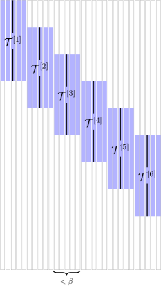
(a) $\varrho=3$ and $\beta=5$ case

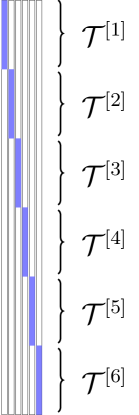
(b) $\varrho=1$ and $\beta=1$ case

Figure 2: Examples of Model 2.3. (a) shows a 1D video object of length $s$ that moves by at least $s/3$ pixels once every $5$ frames. (b) shows the object moving by $s$ at every frame. (b) is an example of the best case for our result - the case with smallest $\rho,\beta$ ($\mathcal{T}_{t}$’s mutually disjoint)

II-B Model on the set of missing entries or the outlier support set, $\mathcal{T}_{t}$

Our result requires that the set of missing entries (or the outlier support sets), $\mathcal{T}_{t}$, have some changes over time. We give one simple model for it below. One example that satisfies this model is a video application consisting of a foreground with one object of length $s$ or less that can remain static for at most $\beta$ frames at a time. When it moves, it moves downwards (or upwards, but always in one direction) by at least $s/\rho$ pixels, and at most $s/\rho_{2}$ pixels. Once it reaches the bottom of the scene, it disappears. The maximum motion is such that, if the object were to move at each frame, it still does not go from the top to the bottom of the scene in a time interval of length $\alpha$, i.e. $\frac{s}{\rho_{2}}\alpha\leq n$. Anytime after it has disappeared another object could appear. We show this example in Fig. 2.

Model 2.3 (model on $\mathcal{T}_{t}$).

Let $t^{k}$, with $t^{k}<t^{k+1}$, denote the times at which $\mathcal{T}_{t}$ changes and let $\mathcal{T}^{[k]}$ denote the distinct sets. For an integer $\alpha$ (we set its value in Theorem 2.7), assume the following.

1. Assume that $\mathcal{T}_{t}=\mathcal{T}^{[k]}$ for all times $t\in[t^{k},t^{k+1})$ with $(t^{k+1}-t^{k})<\beta$ and $|\mathcal{T}^{[k]}|\leq s$.

2. Let $\rho$ be a positive integer so that for any $k$,

   $$\mathcal{T}^{[k]}\cap\mathcal{T}^{[k+\rho]}=\emptyset;$$

   assume that

   $${\rho}^{2}\beta\leq 0.01\alpha.$$

3. For any $k$,

   $$\sum_{i=k+1}^{k+\alpha}\left|\mathcal{T}^{[i]}\setminus\mathcal{T}^{[i+1]}\right|\leq n$$

   and for any $k<i\leq k+\alpha$,

   $$(\mathcal{T}^{[k]}\setminus\mathcal{T}^{[k+1]})\cap(\mathcal{T}^{[i]}\setminus\mathcal{T}^{[i+1]})=\emptyset.$$

   (One way to ensure $\sum_{i=k+1}^{k+\alpha}|\mathcal{T}^{[i]}\setminus\mathcal{T}^{[i+1]}|\leq n$ is to require that for all $i$, $|\mathcal{T}^{[i]}\setminus\mathcal{T}^{[i+1]}|\leq\frac{s}{\rho_{2}}$ with $\frac{s}{\rho_{2}}\alpha\leq n$.)

In this model, $k$ takes values $1,2,\dots$; the largest value it can take is $t_{\max}$ (this will happen if $\mathcal{T}_{t}$ changes at every time).

Clearly the video moving object example satisfies the above model as long as $\rho^{2}\beta\leq 0.01\alpha$. This becomes clearer from Fig. 2.

II-C Denseness

In order to recover the $\bm{\ell}_{t}$’s from missing data or to separate them from the sparse outliers, the basis vectors for the subspace from which they are generated cannot be sparse. We quantify this using the incoherence condition from [2]. Let $\mu$ be the smallest real number such that

$$\max_{i}\|{\bm{P}_{t_{0}}}^{\prime}\bm{I}_{i}\|_{2}^{2}\leq\frac{\mu r_{0}}{n}\quad\text{ and }\quad\max_{i}\|{\bm{P}_{t_{j},\mathrm{new}}}^{\prime}\bm{I}_{i}\|_{2}^{2}\leq\frac{\mu r_{j,\mathrm{new}}}{n}\text{ for all }j$$ (7)

Recall from the notation section that $\bm{I}_{i}$ is the $i^{\text{th}}$ column of the identity matrix (or $i^{\text{th}}$ standard basis vector). We bound $\mu r_{0}$ and $\mu r_{j,\mathrm{new}}$ in the theorem.

II-D Main Result for Online Matrix Completion

Definition 2.4.

Recall that $r_{j,\mathrm{new}}:=\operatorname{rank}(\bm{P}_{t_{j},\mathrm{new}})$ and $r_{j}:=\operatorname{rank}(\bm{P}_{t_{j}})$. Define $r_{\mathrm{new}}:=\max_{j}r_{j,\mathrm{new}}$, and $r=r_{0}+Jr_{\mathrm{new}}$.

Also define $\bm{a}_{t}:={\bm{P}_{t}}^{\prime}\bm{\ell}_{t}$, and for $t\in[t_{j},t_{j+1})$, $\bm{a}_{t,\mathrm{new}}:={\bm{P}_{t_{j},\mathrm{new}}}^{\prime}\bm{\ell}_{t}$. Let

$$\gamma:=\max_{t}\|\bm{a}_{t}\|_{\infty}\quad\text{ and }\quad\gamma_{\mathrm{new}}:=\max_{j}\max_{t\in[t_{j},t_{j}+d]}\|\bm{a}_{t,\mathrm{new}}\|_{\infty}$$

Notice that $\operatorname{rank}(\bm{L})=\operatorname{rank}(\bm{P}_{t_{\max}})\leq r$. Also, $\|\bm{a}_{t}\|_{2}\leq\sqrt{r}\gamma$ and for $t\in[t_{j},t_{j}+d]$, $\|\bm{a}_{t,\mathrm{new}}\|_{2}\leq\sqrt{r_{\mathrm{new}}}\gamma_{\mathrm{new}}$.

The following theorem gives a correctness result for Algorithm 1 given and explained in Section IV. The algorithm has two parameters - $\alpha$ and $K$. The parameter $\alpha$ is the number of consecutive time instants that are used to obtain an estimate of the new subspace, and $K$ is the total number of times the new subspace is estimated before we get an accurate enough estimate of it. The algorithm uses ${\hat{\lambda}_{\mathrm{train}}^{-}}$ and $\hat{\bm{P}}_{t_{\mathrm{train}}}$ defined in Definition 2.1 and $\bm{m}_{t}$ as inputs.

Theorem 2.5.

Consider Algorithm 1. Assume that $\bm{m}_{t}$ satisfies (1). Pick a $\zeta$ that satisfies

$$\zeta\leq\min\left\{\frac{10^{-4}}{r^{2}},\frac{0.03{\hat{\lambda}_{\mathrm{train}}^{-}}}{r^{2}\lambda^{+}},\frac{1}{r^{3}\gamma^{2}},\frac{{\hat{\lambda}_{\mathrm{train}}^{-}}}{r^{3}\gamma^{2}}\right\}.$$

Suppose that the following hold.

1. $\mathrm{dif}(\hat{\bm{P}}_{t_{\mathrm{train}}},\bm{P}_{t_{\mathrm{train}}})\leq r_{0}\zeta$ (notice from Model 2.2 that $\bm{P}_{t_{\mathrm{train}}}=\bm{P}_{t_{0}}=\bm{P}_{1}$);

2. The algorithm parameters are set as:
   $K=\left\lceil\frac{\log(0.16r_{\mathrm{new}}\zeta)}{\log(0.83)}\right\rceil$; and $\alpha=C(\log(6(K+1)J)+11\log(n))$ for a constant

   $$C\geq C_{\mathrm{add}}:={32\cdot 100^{2}}\frac{\max\{16,1.2(\sqrt{\zeta}+\sqrt{r_{\mathrm{new}}}\gamma_{\mathrm{new}})^{4}\}}{\left(r_{\mathrm{new}}\zeta{\hat{\lambda}_{\mathrm{train}}^{-}}\right)^{2}};$$ (8)

3. (Subspace change) Model 2.2 on $\bm{\ell}_{t}$ holds;

4. (Changes in the missing/corrupted sets $\mathcal{T}_{t}$) Model 2.3 on $\mathcal{T}_{t}$ holds or its generalization, Model 5.1 (given in Section V), holds;

5. (Denseness and bound on $s$, $r_{0}$, $r_{\mathrm{new}}$) the bounds in (7) hold with $2s(r_{0}+Jr_{\mathrm{new}})\mu\leq{0.09n}$ and $2sr_{\mathrm{new}}\mu\leq{0.0004n}$;

Then, with probability at least $1-n^{-10}$, at all times $t$,

1. $\|\hat{\bm{\ell}}_{t}-\bm{\ell}_{t}\|_{2}\leq 1.2\left(\sqrt{\zeta}+\sqrt{r_{\mathrm{new}}}\gamma_{\mathrm{new}}\right)$

2. the subspace error $\mathrm{SE}_{t}:=\|(\bm{I}-\hat{\bm{P}}_{t}\hat{\bm{P}}_{t}{}^{\prime})\bm{P}_{t}\|_{2}$ is bounded above by $10^{-2}\sqrt{\zeta}$ for $t\in[t_{j}+d,t_{j+1})$.

Proof.

The proof is given in Sections VI and VII. As shown in Lemma 5.2, Model 2.3 is a special case of Model 5.1 (Model 5.1 is more general) on $\mathcal{T}_{t}$. Hence we prove the result only using Model 5.1. ∎

Theorem 2.5 says that if an accurate estimate of the initial subspace is available; the two algorithm parameters are set appropriately; the $\bm{\ell}_{t}$’s are mutually independent over time and the low-dimensional subspace from which $\bm{\ell}_{t}$ is generated changes “slowly” enough, i.e. (a) the delay between change times is large enough ($d\geq(K+2)\alpha$) and (b) the eigenvalues along the newly added directions are small enough for $d$ frames after a subspace change (so that (5) holds); the set of missing entries at time $t$, $\mathcal{T}_{t}$, has enough changes; and the basis vectors that span the low-dimensional subspaces are dense enough; then, with high probability (w.h.p.), the error in estimating $\bm{\ell}_{t}$ will be small at all times $t$. Also, the error in estimating the low-dimensional subspace will be initially large when new directions are added, but will decay to a small constant times $\sqrt{\zeta}$ within a finite delay.

Consider the accurate initial subspace assumption. If the training data truly satisfies $\bm{m}_{t}=\bm{\ell}_{t}$ (without any noise or modeling error) and if we have at least $r_{0}$ linearly independent $\bm{\ell}_{t}$’s (if $\bm{\ell}_{t}$’s are continuous random vectors, this corresponds to needing $t_{\mathrm{train}}\geq r_{0}$ almost surely), then the estimate of $\operatorname{range}(\bm{P}_{t_{\mathrm{train}}})$ obtained from training data will actually be exact, i.e. we will have $\mathrm{dif}(\hat{\bm{P}}_{t_{\mathrm{train}}},\bm{P}_{t_{\mathrm{train}}})=0$. The theorem assumption that $\mathrm{dif}(\hat{\bm{P}}_{t_{\mathrm{train}}},\bm{P}_{t_{\mathrm{train}}})\leq r_{0}\zeta$ allows for the initial training data to be noisy or not exactly satisfying the model. If the training data is noisy, we need to know $r_{0}$ (in practice this is computed by thresholding to retain a certain percentage of largest eigenvalues). In this case we can let ${\hat{\lambda}_{\mathrm{train}}^{-}}$ be the $r_{0}$-th eigenvalue of $\frac{1}{\alpha}\sum_{t=1}^{t_{\mathrm{train}}}\bm{m}_{t}{\bm{m}_{t}}^{\prime}$ and $\hat{\bm{P}}_{t_{\mathrm{train}}}$ be the $r_{0}$ top eigenvectors.

The following corollary is also proved when we prove the above result.

Corollary 2.6.

The following conclusions also hold under the assumptions of Theorem 2.7 with probability at least $1-n^{-10}$

1. The estimates of the subspace change times given by Algorithm 1 satisfy $t_{j}\leq\hat{t}_{j}\leq t_{j}+2\alpha$, for $j=1,\dots,J$;

2. The estimates of the number of new directions are correct, i.e. $\hat{r}_{j,\mathrm{new},k}=r_{j,\mathrm{new}}$ for $j=1,\dots,J$ and $k=1,\dots,K$;

3. The recovery error satisfies:

   $$\|\hat{\bm{\ell}}_{t}-\bm{\ell}_{t}\|_{2} \leq\begin{cases}1.2\left(\sqrt{\zeta}+\sqrt{r_{\mathrm{new}}}\gamma_{\mathrm{new}}\right)&t\in\left[t_{j},\hat{t}_{j}\right]\\ 1.2\left(1.84\sqrt{\zeta}+(0.83)^{k-1}\sqrt{r_{\mathrm{new}}}\gamma_{\mathrm{new}}\right)&t\in\left[\hat{t}_{j}+(k-1)\alpha,\hat{t}_{j}+k\alpha-1\right],\ k=1,2,\dots,K\\ 2.4\sqrt{\zeta}&t\in\left[\hat{t}_{j}+K\alpha,t_{j+1}-1\right];\end{cases}$$

4. The subspace error satisfies,

   $$\mathrm{SE}_{t}\leq\begin{cases}1&t\in\left[t_{j},\hat{t}_{j}\right]\\ 10^{-2}\sqrt{\zeta}+0.83^{k-1}&t\in\left[\hat{t}_{j}+(k-1)\alpha,\hat{t}_{j}+k\alpha-1\right],\ k=1,2,\dots,K\\ 10^{-2}\sqrt{\zeta}&t\in\left[\hat{t}_{j}+K\alpha,t_{j+1}-1\right].\end{cases}$$

II-E Main Result for Online Robust PCA

Recall that in this case we assume that the observations $\bm{m}_{t}$ satisfy $\bm{m}_{t}=\bm{\ell}_{t}+\bm{x}_{t}$ with the support of $\bm{x}_{t}$, denoted $\mathcal{T}_{t}$, not known. We have the following result for Algorithm 2 given and explained in Section IV. This requires two extra assumptions beyond what the previous result needed. For the matrix completion problem, the set of missing entries is known, while in the robust PCA setting, the support set, $\mathcal{T}_{t}$, of the sparse outliers, $\bm{x}_{t}$, must be determined. We recover this using an ell-1 minimization step followed by thresholding. To do this correctly, we need a lower bound on the absolute values of the nonzero entries of $\bm{x}_{t}$. Moreover, Algorithm 2 has two extra parameters - $\xi$, which is the bound on the two norm of the noise seen by the ell-1 minimization step, and $\omega$, which is the threshold used to recover the support of $\bm{x}_{t}$. These need to be set appropriately.

Theorem 2.7.

Consider Algorithm 2. Assume that $\bm{m}_{t}$ satisfies (2) and assume everything else in Theorem 2.5. Also assume

1. The two extra algorithm parameters are set as: $\xi=\sqrt{r_{\mathrm{new}}}\gamma_{\mathrm{new}}+(\sqrt{r}+\sqrt{r_{\mathrm{new}}})\sqrt{\zeta}$ and $\omega=7\xi$

2. We have $x_{\min}:=\min_{t}\min_{i:(\bm{x}_{t})_{i}\neq 0}|(\bm{x}_{t})_{i}|>14\xi$

Then with probability at least $1-n^{-10}$,

1. all conclusions of Theorem 2.5 and Corollary 2.6 hold;

2. the support set $\mathcal{T}_{t}$ is exactly recovered, i.e. $\hat{\mathcal{T}}_{t}=\mathcal{T}_{t}$ for all $t$;

3. $\|\bm{x}_{t}-\hat{\bm{x}}_{t}\|_{2}=\|\bm{\ell}_{t}-\hat{\bm{\ell}}_{t}\|_{2}$ and $\|\bm{\ell}_{t}-\hat{\bm{\ell}}_{t}\|_{2}$ satisfies the bounds given in Theorem 2.5 and Corollary 2.6.

The second assumption above can be interpreted as either a lower bound on $x_{\min}$, or as an upper bound on $\sqrt{r_{\mathrm{new}}}\gamma_{\mathrm{new}}$ in terms of $x_{\min}$. This latter interpretation is another “slow subspace change” condition. For the $\bm{x}_{t}$’s, this result shows that their support is exactly recovered w.h.p. and its nonzero entries are accurately recovered.

II-F Simple Generalizations

Model on $\ell_{t}$. Consider the subspace change model, Model 2.2. For simplicity we put a slow increase model on the eigenvalues along the new directions for the entire period $[t_{j},t_{j+1})$. However, as explained below the model, the proof of our result does not actually use this slow increase model. It only uses (5), i.e. ${\hat{\lambda}_{\mathrm{train}}^{-}}\leq\lambda_{\mathrm{new}}^{-}\leq\lambda_{\mathrm{new}}^{+}\leq 3{\hat{\lambda}_{\mathrm{train}}^{-}}$. Recall that $\lambda_{\mathrm{new}}^{-}$ and $\lambda_{\mathrm{new}}^{+}$ are the minimum and maximum eigenvalues along the new directions for the first $d$ frames after a subspace change. Thus, in the interval $[t_{j}+d+1,t_{j+1})$ our proof actually does not need any constraint on $\bm{\Lambda}_{t,\mathrm{new}}$.

With a minor modification to our proof, we can prove our result with an even weaker condition. We need (5) to hold with $\lambda_{\mathrm{new}}^{-}$ being the minimum of the minimum eigenvalues of any $\alpha$-frame average covariance matrix along the new directions over the period $[t_{j},t_{j}+d]$, i.e. with $\lambda_{\mathrm{new}}^{-}=\min_{j}\min_{\tau\in[t_{j},t_{j}+d-\alpha]}\lambda_{\min}(\frac{1}{\alpha}\sum_{t=\tau}^{\tau+\alpha-1}\bm{\Lambda}_{t,\mathrm{new}})$. For video analytics, this translates to requiring that, after a subspace change, enough (but not necessarily all) background frames have ‘detectable’ energy along the new directions, so that the minimum eigenvalue of the average covariance is above a threshold.

Secondly, we should point out that there is a trade off between the bound on $q_{i}{v_{i}}^{d}$, and consequently on $\lambda_{\mathrm{new}}^{+}$, in Model 2.2 and the bound on ${\rho}^{2}\beta$ assumed in Model 2.3. Allowing a larger value of $q_{i}{v_{i}}^{d}$ (faster subspace change) will require a tighter bound on $\rho^{2}\beta$ which corresponds to requiring more changes to $\mathcal{T}_{t}$. We chose the bounds $q_{i}(v_{i})^{d}\leq 3$ and $\rho^{2}\beta\leq.01\alpha$ for simplicity of computations. There are many other pairs that would also work. The above trade-off can be seen from the proof of Lemma 6.14. The proof uses Model 5.1 of which Model 2.3 is a special case. For video analytics, this means that if the background subspace changes are faster, then we also need the foreground objects to be moving more so we can ‘see’ enough of the background behind them.

Thirdly, in Model 2.2 we let $\bm{P}_{t}\bm{\Lambda}_{t}{\bm{P}_{t}}^{\prime}$ be an EVD of $\bm{\Sigma}_{t}$. This automatically implies that $\bm{\Lambda}_{t}$ is diagonal. But our proof only uses the fact that $\bm{\Lambda}_{t}$ is block diagonal with blocks $\bm{\Lambda}_{t,*}$ and $\bm{\Lambda}_{t,\mathrm{new}}$. If we relax this and we let $\bm{P}_{t}\bm{\Lambda}_{t}{\bm{P}_{t}}^{\prime}$ be a decomposition of $\bm{\Sigma}_{t}$ where $\bm{\Lambda}_{t}$ is block diagonal as above, then our model allows the variance along any direction from $\operatorname{range}(\bm{P}_{t_{j}-1})$ to become zero for any period of time and/or become nonzero again later. Thus, in the special case of (6) we can actually allow $\bm{P}_{t}=[(\bm{P}_{t-1}\bm{R}_{t}\setminus\bm{P}_{t,\mathrm{del}})\ \ \bm{P}_{t,\mathrm{new}}]$, where $\bm{R}_{t}$ is an $r_{j-1}\times r_{j-1}$ rotation matrix and $\bm{P}_{t,\mathrm{del}}$ contains the columns of $\bm{P}_{t-1}\bm{R}_{t}$ for which the variance is zero. This will be a special case of this generalization if $[\bm{P}_{t_{1}-1}\ \bm{P}_{t_{1},\mathrm{new}}\ \bm{P}_{t_{2},\mathrm{new}}\ \dots\ \bm{P}_{t_{J},\mathrm{new}}]$ is a basis matrix.

Initialization condition. The first condition of the theorem requires that we have accurate initial subspace knowledge. As explained below the theorem, this means that we can allow noisy training data. Moreover, notice that if we let $t_{1}=t_{\mathrm{train}}+1$, then new background directions can enter the subspace at the same time as the first foreground object. Said another way, all we need is an accurate enough estimate of all but $r_{\mathrm{new}}$ directions of the initial subspace, and an assumption of small eigenvalues for sometime ($d$ frames) along the directions for which we do not have an accurate enough estimate (or do not have an estimate).

Denseness assumption. Consider the denseness assumption. Define the (un)denseness coefficient as follows.

Definition 2.8.

For a basis matrix $\bm{P}$, define $\displaystyle\kappa_{s}(\bm{P}):=\max_{|\mathcal{T}|\leq s}\|{\bm{I}_{\mathcal{T}}}^{\prime}\bm{P}\|_{2}$.

Notice that left hand side in (7) is $\left[\kappa_{1}(\bm{P})\right]^{2}$. Using the triangle inequality, it is easy to show that $\kappa_{s}(\bm{P})\leq\sqrt{s}\kappa_{1}(\bm{P})$ [12]. Therefore, using the fact that for a basis matrix $[\bm{P}_{1}\ \bm{P}_{2}]$, $(\kappa_{s}([\bm{P}_{1}\ \bm{P}_{2}]))^{2}\leq(\kappa_{s}(\bm{P}_{1}))^{2}+(\kappa_{s}(\bm{P}_{2}))^{2}$ (see proof of the first statement of Lemma C.2 in Appendix C), the denseness assumptions of Theorem 2.7 imply that

$$\kappa_{s,*}:=\kappa_{2s}(\bm{P}_{t_{J}})\leq 0.3\quad\text{ and }\quad\kappa_{s,\mathrm{new}}:=\max_{j}\kappa_{2s}(\bm{P}_{t_{j},\mathrm{new}})\leq 0.02.$$ (9)

The proof of Theorem 2.7 only uses (9) for the denseness assumption.

The reason for defining $\kappa_{s}$ as above is the following lemma from [12].

Lemma 2.9 ([12]).

For a basis matrix $\bm{P}$, $\delta_{s}(\bm{I}-\bm{P}\bm{P}^{\prime})=\left(\kappa_{s}(\bm{P})\right)^{2}$.

Lower bound on minimum nonzero entry of $x_{t}$ in the online RPCA result (Corollary 2.7). For online RPCA, notice that our result needs a lower bound on the minimum magnitude nonzero entry, $x_{\min}$, of the outlier vector $x_{t}$. This may seem counter-intuitive, since it means that outlier magnitudes need to be large enough for the proposed algorithm to work whereas one would expect that smaller corruptions are easier to deal with. This is actually true in our case as well, and the lower bound on minimum nonzero entry of $x_{t}$ is an artifact of trying to use a simpler model and a simpler proof approach. As we explain next, what we really need is that the corruptions either be small enough (to not affect subspace recovery too much) or be large enough (to be detectable).

Corollary 2.10 (No lower bound on outlier magnitude).

Consider Algorithm 2. Assume that $\bm{m}_{t}$ satisfies (2). Assume that the following hold:

1. Suppose that $\bm{x}_{t}$ and $\bm{\ell}_{t}$ are mutually independent; and there exists a partition of $\mathcal{T}_{t}$ into $\mathcal{T}_{t,\mathrm{large}},\mathcal{T}_{t,\mathrm{small}}$ so that

   • $\min_{t}\min_{i\in\mathcal{T}_{t,\mathrm{large}}}|(\bm{x}_{t})_{i}|-14\max_{t}\|(\bm{x}_{t})_{\mathcal{T}_{t,\mathrm{small}}}\|_{2}>14(\sqrt{r_{\mathrm{new}}}\gamma_{\mathrm{new}}(d)+(\sqrt{r}+\sqrt{r_{\mathrm{new}}})\sqrt{\zeta})$

   • and $\max_{t}\|(\bm{x}_{t})_{\mathcal{T}_{t,\mathrm{small}}}\|_{2}^{2}\leq 0.03\zeta{\hat{\lambda}_{\mathrm{train}}^{-}}$

   Let $\epsilon_{w}:=\max_{t}\|(\bm{x}_{t})_{\mathcal{T}_{t,\mathrm{small}}}\|_{2}$.

2. Algorithm parameters are set as $\xi=\epsilon_{w}+\sqrt{r_{\mathrm{new}}}\gamma_{\mathrm{new}}+(\sqrt{r}+\sqrt{r_{\mathrm{new}}})\sqrt{\zeta}$; $\omega=7\xi$; $K=\left\lceil\frac{\log(0.16r_{\mathrm{new}}\zeta)}{\log(0.83)}\right\rceil$; and $\alpha\geq{32\cdot 100^{2}}\frac{\max\{16,1.2(\sqrt{\zeta}+\sqrt{r_{\mathrm{new}}}\gamma_{\mathrm{new}}+\epsilon_{w})^{4}\}}{\left(r_{\mathrm{new}}\zeta{\hat{\lambda}_{\mathrm{train}}^{-}}\right)^{2}}(\log(6(K+1)J)+11\log n)$;

3. Everything else in Theorem 2.5 holds with $\mathcal{T}_{t}$ replaced by $\mathcal{T}_{t,\mathrm{large}}$.

Then, with probability at least $1-n^{-10}$, the support set of the large entries of $x_{t}$, $\mathcal{T}_{t,\mathrm{large}}$, is exactly recovered at all times, $\|\bm{x}_{t}-\hat{\bm{x}}_{t}\|_{2}=\|\bm{\ell}_{t}-\hat{\bm{\ell}}_{t}\|_{2}\leq 1.2\left(\sqrt{\zeta}+\sqrt{r_{\mathrm{new}}}\gamma_{\mathrm{new}}+\epsilon_{w}\right)$ and and all other conclusions of Theorem 2.5 hold.

Proof.

The proof will follow in exactly the same fashion as the proof of the original theorem. We will just need to treat $(x_{t})_{\mathcal{T}_{t,\mathrm{small}}}$ as an extra “noise” term and use one of the following three facts at various places. Let $\mathbb{E}[.]$ denote expectation conditioned on accurate recovery so far and on $\mathcal{T}_{t}$ (this is formally defined in the proofs). We will use (a) $\|(\bm{x}_{t})_{\mathcal{T}_{t,\mathrm{small}}}\|_{2}\leq\epsilon_{w}\leq\sqrt{0.03\zeta{\hat{\lambda}_{\mathrm{train}}^{-}}}$; (b) $\mathbb{E}[\bm{\ell}_{t}(\bm{x}_{t})_{\mathcal{T}_{t,\mathrm{small}}}{}^{\prime}]=0$ (this follows because $\bm{\ell}_{t}$ is zero mean and $\bm{\ell}_{t}$ and $\bm{x}_{t}$ are independent (and hence $\bm{\ell}_{t}$ and $\{\mathcal{T}_{t},(\bm{x}_{t})_{\mathcal{T}_{t,\mathrm{small}}}\}$ are independent)); and (c) $\|\mathbb{E}[(\bm{x}_{t})_{\mathcal{T}_{t,\mathrm{small}}}(\bm{x}_{t})_{\mathcal{T}_{t,\mathrm{small}}}{}^{\prime}]\|_{2}\leq\max_{t}\|(x_{t})_{\mathcal{T}_{t,\mathrm{small}}}(\bm{x}_{t})_{\mathcal{T}_{t,\mathrm{small}}}{}^{\prime}\|_{2}\leq\epsilon_{w}^{2}\leq 0.03\zeta{\hat{\lambda}_{\mathrm{train}}^{-}}$. ∎

III Discussion

III-A Discussion of the assumptions used

In the previous section, we provide two related results, one for online matrix completion (MC) and the second for online robust PCA (RPCA). The result for online RPCA can also be interpreted as a result for online sparse matrix recovery in (potentially) large but structured noise $\bm{\ell}_{t}$. Notice that our result does not require an upper bound on $\lambda^{+}$ (the maximum eigenvalue of $\operatorname{Cov}(\bm{\ell}_{t})$ at any time) or on $\gamma$ (the bound on the maximum magnitude of any entry of $\bm{P}_{t}^{\prime}\bm{\ell}_{t}$ for any time $t$). Both these parameters are only used to select $\zeta$, which in turn governs the value of $K$ and $\alpha$ and hence governs the required delay between subspace change times.

Our results require accurate initial subspace knowledge. As explained earlier, for video analytics, this corresponds to requiring an initial short sequence of background-only video frames whose subspace can be estimated via SVD (followed by using a singular value threshold to retain a certain number of top left singular vectors). Alternatively if an initial short sequence of the video data satisfies the assumptions required by a batch method such as PCP (for RPCA) and NNM (for MC), that can be used to estimate the low-rank part, followed by SVD to get the column subspace. For online MC, another alternative is to use the initialization techniques of GROUSE [8] or PETRELS [9] or to use the adaptive MC idea of [11].

In Model 2.2, we are placing a slow increase assumption on the eigenvalues along the new directions, $\bm{P}_{t_{j},\mathrm{new}}$, for the interval $[t_{j},t_{j+1})$. Thus after $t_{j+1}$, the eigenvalues along $\bm{P}_{t_{j},\mathrm{new}}$ can increase gradually or suddenly to any large value up to $\lambda^{+}$. In fact as explained above, our proof needs the slow increase to hold only for the first $d$ time instants after $t_{j}$, so, in fact, at any time after $t_{j}+d$, the eigenvalues along $\bm{P}_{t_{j},\mathrm{new}}$ could increase to a large value.

Model 2.3 on $\mathcal{T}_{t}$ is a practical model for moving foreground objects in video. We should point out that this model is one special case of the general set of conditions we need (Model 5.1). Some other special cases of it are discussed in Section IX.

The model on $\mathcal{T}_{t}$ (Model 2.3) and the denseness condition of the theorem constrain $s$ and $s,r_{0},r_{\mathrm{new}},J$ respectively. Model 2.3 requires $s\leq\rho_{2}n/\alpha$ for a constant $\rho_{2}$. Using the expression for $\alpha$, it is easy to see that as long as $J\in\mathcal{O}(n)$, we have $\alpha\in\mathcal{O}(\log n)$ and so Model 2.3 needs $s\in\mathcal{O}(\frac{n}{\log n})$. With $s\in\mathcal{O}(\frac{n}{\log n})$, the denseness condition will hold if $r_{0}\in\mathcal{O}(\log n)$, $J\in\mathcal{O}(\log n)$ and $r_{\mathrm{new}}$ is a constant. This is one set of sufficient conditions that we allow on the rank-sparsity product.

III-B Comparison with the results for PCP and NNM

Let $\bm{L}:=[\bm{\ell}_{1},\bm{\ell}_{2},\dots,\bm{\ell}_{t_{\max}}]$ and $\bm{S}:=[\bm{x}_{1},\bm{x}_{2},\dots,\bm{x}_{t_{\max}}]$. Let $r_{\text{mat}}:=\operatorname{rank}(\bm{L})$. Clearly $r_{\text{mat}}\leq r_{0}+Jr_{\mathrm{new}}$ and the bound is tight. Let $s_{\text{mat}}:=t_{\max}s$ be a bound on the total number of missing entries of $\bm{L}$ or on the support size of the outliers’ matrix $\bm{S}$. In terms of $r_{\text{mat}}$ and $s_{\text{mat}}$, what we need is $r_{\text{mat}}\in\mathcal{O}(\log n)$ and $s_{\text{mat}}\in\mathcal{O}(\frac{nt_{\max}}{\log n})$. This is stronger than what the PCP result from [2] or the result for NNM from [6] need (e.g., the PCP result from [2] allows $r_{\text{mat}}\in\mathcal{O}\left(\frac{n}{(\log n)^{2}}\right)$ while allowing $s_{\text{mat}}\in\mathcal{O}(nt_{\max})$), but is similar to what the PCP results from [3, 4] need.

Other disadvantages of our result are as follows. (1) Our result needs accurate initial subspace knowledge and slow subspace change of $\bm{\ell}_{t}$. As explained earlier and in [12, Fig. 6], both of these are often practically valid for video analytics applications. Moreover, we also need the $\bm{\ell}_{t}$’s to be zero mean and mutually independent over time. Zero mean is achieved by letting $\bm{\ell}_{t}$ be the background image at time $t$ with an empirical ‘mean background image’, computed using the training data, subtracted out. The independence assumption then models independent background variations around a common mean. As we explain in Section IX, this can be easily relaxed and we can get a result very similar to the current one under a first order autoregressive model on the $\bm{\ell}_{t}$’s. (2) Moreover, Algorithms 1 and 2 need multiple algorithm parameters to be appropriately set. The PCP or NNM results need this for none [2, 6] or at most one [3, 4] algorithm parameter. (3) Thirdly, our result for online RPCA also needs a lower bound on $x_{\min}$ while the PCP results do not need this. (4) Moreover, even with this, we can only guarantee accurate recovery of $\bm{\ell}_{t}$, while PCP or NNM guarantee exact recovery.

(1) The advantage of our work is that we analyze an online algorithm (ReProCS) that is faster and needs less storage compared with PCP or NNM. It needs to store only a few $n\times\alpha$ or $n\times r_{\text{mat}}$ matrices, thus the storage complexity is $\mathcal{O}(n\log n)$ while that for PCP or NNM is $\mathcal{O}(nt_{\max})$. In general $t_{\max}$ can be much larger than $\log n$. (2) Moreover, we do not need any assumption on the right singular vectors of $\bm{L}$ while all results for PCP or NNM do. (3) Most importantly, our results allow highly correlated changes of the set of missing entries (or outliers). From the assumption on $\mathcal{T}_{t}$, it is easy to see that we allow the number of missing entries (or outliers) per row of $\bm{L}$ to be $\mathcal{O}(t_{\max})$ as long as the sets follow Model 2.3. The PCP results from [3, 4] need this number to be $\mathcal{O}(\frac{t_{\max}}{r_{\text{mat}}})$ which is stronger. The PCP result from [2] or the NNM result [6] need an even stronger condition - they need the set $(\cup_{t=1}^{t_{\max}}\mathcal{T}_{t})$ to be generated uniformly at random.

III-C Other results for online RPCA and online MC

Our online RPCA result improves upon the online RPCA results from our earlier work [12] for two reasons. First, the result of [12] was a partial result because it required a denseness assumption on $(\bm{I}-\bm{P}_{t_{j},\mathrm{new}}{\bm{P}_{t_{j},\mathrm{new}}}^{\prime})\hat{\bm{P}}_{t}$ and $(\bm{I}-\hat{\bm{P}}_{t,*}\hat{\bm{P}}_{t,*}{}^{\prime}-\hat{\bm{P}}_{t,\mathrm{new}}\hat{\bm{P}}_{t,\mathrm{new}}{}^{\prime})\bm{P}_{t_{j},\mathrm{new}}$. Here $\hat{\bm{P}}_{t,*}$ and $\hat{\bm{P}}_{t,\mathrm{new}}$ are estimates computed by Algorithm 2. Thus, the result depended on intermediate algorithm estimates satisfying certain properties. In this work, we remove this requirement and instead provide a complete correctness result. The extra assumption that we need is Model 2.3 on $\mathcal{T}_{t}$ (or its generalization given in Model 5.1 later). Secondly, we provide a correctness result for a ReProCS-based algorithm that detects subspace change automatically and also estimates the rank of the new subspace automatically. The algorithm studied in [12] required knowing $t_{j}$ and $r_{j,\mathrm{new}}$ exactly for each $j$. Algorithms 1 and 2 in this work only require upper bounds on $r_{\mathrm{new}}$, $\gamma_{\mathrm{new}}$ and $J$ (these are needed to set the algorithm parameters - $\alpha$ and $K$ for Algorithm 1, and also $\xi$ and $\omega$ for Algorithm 2) and a small enough $\zeta$ (need bounds on $r$, $\lambda^{+}$ and $\gamma$ to set this). A third minor advantage is that we also provide an algorithm and a result for online MC.

The proof of our results adapts the overall framework developed in [12]. The two important additions are: (a) Model 5.1 and Lemma 5.3 for it, and the way it is used in the proof of Lemma 6.23; and (b) the detection lemma (Lemma 6.17), the no false detection lemma (Lemma 6.16) and the p-PCA lemma (Lemma 6.18) and the lemmas used to prove these. (a) allows us to get a complete correctness result; (b) allows us to analyze an algorithm that does not use knowledge of $t_{j}$ or $r_{j,\mathrm{new}}$.

In [20], Feng et. al. propose a method for online RPCA and prove a partial result for their algorithm. The approach is to reformulate the PCP program and use this reformulation to develop a recursive algorithm that converges asymptotically to the solution of PCP as long as the basis estimate $\hat{\bm{P}}_{t}$ is full rank at each time $t$. Since this result assumes something about the algorithm estimates, it is also only a partial result.

Another recent work that uses knowledge of the initial subspace estimate and performs recovery in a piecewise batch fashion is modified-PCP [21]. However, like PCP, the result for modified PCP also needs uniformly randomly generated support sets. Its advantage is that its assumption on the rank-sparsity product is weaker than that of PCP, and hence weaker than that needed by this work. A detailed simulation comparison between modified-PCP, ReProCS and PCP demonstrating both these things is available in [21, Fig. 6].

Some other recent works that also study the online MC problem (defined differently from how we define it) include [7], Grassmanian Rank-One Update Subspace Estimation (GROUSE) [8] and Parallel Subspace Estimation and Tracking by Recursive Least Squares From Partial Observations (PETRELS) [9]. We discuss the connection with [7] in Section IV. GROUSE is a first order stochastic gradient method. It uses rank-one updates to track the underlying subspace on the Grassmannian manifold. A result for its convergence to the local minimum of the cost function it optimizes is obtained in [10]. PETRELS is a second order stochastic gradient method. As explained in [9], in PETRELS, the low-dimensional subspace is tracked by minimizing a geometrically discounted sum of projection residuals on the observed entries at each time index. If missing entries are required then they can be reconstructed via least squares estimation. The subspace is updated recursively so that it is not necessary to retain historical data indefinitely. If the underlying subspace is fixed and the data stream is fully observed, then it is shown that the PETRELS estimate converges to the true subspace. In general, it always converges to the stationary point of the cost function it optimizes [9]. The advantage of PETRELS and GROUSE is that they do not need initial subspace knowledge. For our algorithms, when the initial subspace knowledge is not available or initial complete and outlier-free data is not available, we can also use the PETRELS or GROUSE ideas for initialization.

IV Automatic ReProCS Algorithms for Online MC and Online RPCA and Why They Work

In this section, we first introduce the automatic ReProCS based algorithm for online MC and explain why it works (this also provides the key idea why the proof of our main result would go through). Next, we do the same thing for the online RPCA algorithm. In the last two subsections (Sections IV-C and IV-D), we explain the key insight used by our proof and give the proof outline.

IV-A Automatic ReProCS for Online MC (Algorithm 1)

The model on $\bm{m}_{t}$ from (1) is a special case of that from (2) with $\bm{x}_{t}=-\bm{I}_{{\mathcal{T}}_{t}}\bm{I}_{{\mathcal{T}}_{t}}{}^{\prime}\bm{\ell}_{t}$ and with the support of $\bm{x}_{t}$, $\mathcal{T}_{t}$ known [2]. Thus, we can use a simplification of the ReProCS idea for online RPCA [12] to also solve the online MC problem.

Algorithm 1 proceeds as follows. Let $\hat{\bm{P}}_{t-1}$ denote the basis matrix for the estimate of the subspace where $\bm{\ell}_{t-1}$ lies. If it is an accurate estimate, because of “slow subspace change”, projecting the measurement $\bm{m}_{t}=\bm{x}_{t}+\bm{\ell}_{t}$ onto its orthogonal complement will nullify most of $\bm{\ell}_{t}$. Specifically, we compute $\bm{y}_{t}:=\bm{\Phi}_{t}\bm{m}_{t}$ where $\bm{\Phi}_{t}:=\bm{I}-\hat{\bm{P}}_{t-1}\hat{\bm{P}}_{t-1}{}^{\prime}$. Thus, $\bm{y}_{t}$ can be rewritten as

$$\bm{y}_{t}=\bm{\Phi}_{t}\bm{x}_{t}+\bm{b}_{t}\ \text{where}\ \bm{b}_{t}:=\bm{\Phi}_{t}\bm{\ell}_{t}$$

and it can be argued that $\|\bm{b}_{t}\|_{2}$ is small. Since the support of $\bm{x}_{t}$, $\mathcal{T}_{t}$, is known, we can simply recover its nonzero entries by least squares (LS) estimation, i.e. we get $\hat{\bm{x}}_{t}=\bm{I}_{\mathcal{T}_{t}}(\bm{\Phi}_{t})_{\mathcal{T}_{t}}{}^{\dagger}\bm{y}_{t}$ and then get an estimate of $\bm{\ell}_{t}$ as $\hat{\bm{\ell}}_{t}=\bm{m}_{t}-\hat{\bm{x}}_{t}$. The above approach of recovering $\bm{\ell}_{t}$ is equivalent to that used by Brand in [7], there they recover $\bm{\ell}_{t}$ as an LS estimate of $\hat{\bm{P}}\hat{\bm{P}}^{\prime}\bm{\ell}_{t}\approx\bm{\ell}_{t}$.

Let $\bm{e}_{t}:=\bm{\ell}_{t}-\hat{\bm{\ell}}_{t}$. With the above, it is easy to see that

$$\bm{e}_{t}=\bm{I}_{\mathcal{T}_{t}}(\bm{\Phi}_{t})_{\mathcal{T}_{t}}{}^{\dagger}\bm{b}_{t}=\bm{I}_{\mathcal{T}_{t}}[(\bm{\Phi}_{t})_{\mathcal{T}_{t}}{}^{\prime}(\bm{\Phi}_{t})_{\mathcal{T}_{t}}]^{-1}\bm{I}_{\mathcal{T}_{t}}{}^{\prime}\bm{\Phi}\bm{\ell}_{t}.$$

Using the denseness assumption, it can be argued that the RIC of $\bm{\Phi}_{t}$ will be small (see Lemma 2.9). Under the theorem’s assumptions, and conditioned on accurate recovery so far, we can bound it by 0.14. Thus, $\|(\bm{\Phi}_{t})_{\mathcal{T}_{t}}{}^{\prime}(\bm{\Phi}_{t})_{\mathcal{T}_{t}}^{-1}\|_{2}\leq 1/(1-0.14)<1.2$ and so $\|\bm{e}_{t}\|_{2}\leq 1.2\|\bm{b}_{t}\|_{2}$, i.e. it is small too (see Lemma 6.15).

Projection-PCA (p-PCA). The next step is to use a modification of standard PCA called projection-PCA (p-PCA), to update the subspace estimate. The reason we need p-PCA is this. Let $\sum_{t}$ denote a sum over an $\alpha$ length time interval. In our problem, the error, $\bm{e}_{t}$, in the observation/estimate of $\bm{\ell}_{t}$, $\hat{\bm{\ell}}_{t}$, is correlated with $\bm{\ell}_{t}$. Because of this, the dominant terms in the perturbation seen by standard PCA, $\frac{1}{\alpha}\sum_{t}\hat{\bm{\ell}}_{t}\hat{\bm{\ell}}_{t}{}^{\prime}-\frac{1}{\alpha}\sum_{t}\bm{\ell}_{t}{\bm{\ell}_{t}}^{\prime}$, are $\frac{1}{\alpha}\sum_{t}\bm{\ell}_{t}{\bm{e}_{t}}^{\prime}$ and its transpose. Thus, when the condition number of $\operatorname{Cov}(\bm{\ell}_{t})$ is large, it becomes difficult to argue that the perturbation will be small compared to the smallest eigenvalue of $\operatorname{Cov}(\bm{\ell}_{t})$. With a large perturbation, either the $\sin\theta$ theorem [22] (that bounds the subspace error between the eigenvectors of the true and estimated sample covariance matrices) cannot be applied or it gives a useless bound.

Our proposed approach, projection-PCA (p-PCA) addresses the above issue as follows. At $t=t_{j}$, let $\bm{P}_{*}:=\bm{P}_{t_{j-1}}$, $\bm{P}_{\mathrm{new}}:=\bm{P}_{t_{j},\mathrm{new}}$, and suppose that the subspace $\operatorname{range}(\bm{P}_{*})$ has been accurately recovered, i.e. we have $\hat{\bm{P}}_{*}$ so that $\mathrm{dif}(\hat{\bm{P}}_{*},\bm{P}_{*})\ll 1$. Then at a time at or after $t_{j}+\alpha$ if we project the $\alpha$ previous $\hat{\bm{\ell}}_{t}$’s perpendicular to $\hat{\bm{P}}_{*}$, we will considerably reduce the perturbation seen by the PCA step. We detect subspace change by checking if the maximum singular value of the matrix formed by these projected $\hat{\bm{\ell}}_{t}$’s is above a threshold. Denote the time at which change is detected by ${\hat{t}}_{j}$. After ${\hat{t}}_{j}$ we use SVD on $K$ different sets of $\alpha$ frames of the projected $\hat{\bm{\ell}}_{t}$’s to get improved estimates of the new subspace $\operatorname{range}(\bm{P}_{\mathrm{new}})$ in each iteration. To be precise, we get the $k$-th estimate, $\hat{\bm{P}}_{\mathrm{new},k}$, as the left singular vectors of $(\bm{I}-\hat{\bm{P}}_{*}\hat{\bm{P}}_{*}{}^{\prime})[\hat{\bm{\ell}}_{{\hat{t}}_{j}+(k-1)\alpha+1},\dots,\hat{\bm{\ell}}_{{\hat{t}}_{j}+k\alpha}]$ with singular values above a threshold. After each p-PCA step, we update $\hat{\bm{P}}_{t}$ as $\hat{\bm{P}}_{t}=[\hat{\bm{P}}_{*}\ \textit{}\hat{\bm{P}}_{\mathrm{new},k}]$. Finally at time $t={\hat{t}}_{j}+K\alpha$, we update $\hat{\bm{P}}_{*}$ as $[\hat{\bm{P}}_{*}\ \hat{\bm{P}}_{\mathrm{new},K}]$.

In the subspace update step, Algorithm 1 toggles between the “detect” phase and the “ppca” phase. It starts in the “detect” phase. When a subspace change is detected, i.e. at $t={\hat{t}}_{j}$ it enters the “ppca” phase. After $K$ iterations of p-PCA, i.e. at $t={\hat{t}}_{j}+K\alpha+1$, the new subspace has been accurately estimated and this time it enters the “detect” phase again.

Why p-PCA works. The reason p-PCA works is as follows. Before the first p-PCA step, i.e. for $t\in[t_{j},{\hat{t}}_{j}+\alpha)$, $\hat{\bm{P}}_{t}=\hat{\bm{P}}_{*}$ and thus the noise seen by the projected sparse recovery step, $\bm{b}_{t}=\bm{\Phi}\bm{\ell}_{t}=(\bm{I}-\hat{\bm{P}}_{*}\hat{\bm{P}}_{*}{}^{\prime})\bm{\ell}_{t}$, will be the largest. Hence the error $\bm{e}_{t}$ will also be the largest for the $\hat{\bm{\ell}}_{t}$’s used for the first p-PCA step. However because of the projection perpendicular to $\hat{\bm{P}}_{*}$ and slow subspace change, even this error is not too large. Because of this and because $\bm{e}_{t}$ is sparse and supported on $\mathcal{T}_{t}$ and $\mathcal{T}_{t}$ follows Model 2.3, we can argue that $\hat{\bm{P}}_{\mathrm{new},1}$ is a good estimate, i.e. $\mathrm{dif}([\hat{\bm{P}}_{*}\ \hat{\bm{P}}_{\mathrm{new},1}],\bm{P}_{\mathrm{new}})\leq 0.2<1$. After the first p-PCA step, $\hat{\bm{P}}_{t}=[\hat{\bm{P}}_{*}\ \hat{\bm{P}}_{\mathrm{new},1}]$ and this will reduce $\bm{b}_{t}$ and hence $\bm{e}_{t}$ for the $\hat{\bm{\ell}}_{t}$’s in the next $\alpha$ frames. This and the sparseness of $\bm{e}_{t}$, in turn, will mean that the perturbation seen by the second p-PCA step will be smaller and so $\hat{\bm{P}}_{\mathrm{new},2}$ will be a more accurate estimate of $\operatorname{range}(\bm{P}_{\mathrm{new}})$ than $\hat{\bm{P}}_{\mathrm{new},1}$. This is done $K$ times with $K$ chosen so that $\mathrm{dif}([\hat{\bm{P}}_{*}\ \hat{\bm{P}}_{\mathrm{new},K}],\bm{P}_{\mathrm{new}})\leq r_{\mathrm{new}}\zeta$. By the theorem assumptions, and because we can show $t_{j}\leq{\hat{t}}_{j}<t_{j}+2\alpha$ (we explain this below), it is clear that $t_{j+1}>{\hat{t}}_{j}+K\alpha$. Thus, the new subspace added at $t_{j}$ is accurately estimated before the next change time $t_{j+1}$.

Why ${\hat{t}}_{j}$ are correctly detected. As explained above, we detect subspace changes by comparing the eigenvalues of $(\bm{I}-\hat{\bm{P}}_{*}\hat{\bm{P}}_{*}{}^{\prime})\frac{1}{\alpha}\sum_{t}\hat{\bm{\ell}}_{t}\hat{\bm{\ell}}_{t}{}^{\prime}(\bm{I}-\hat{\bm{P}}_{*}\hat{\bm{P}}_{*}{}^{\prime})$ to a chosen threshold at every $t=u\alpha$ for $u=1,2,\dots,\left\lfloor\frac{t_{\max}}{\alpha}\right\rfloor$ when the algorithm is in the “detect” phase. In order to correctly detect ${\hat{t}}_{j}$, the algorithm first must not falsely detect new directions when none are present and it must detect subspace change within a short delay after it has occurred. The former will occur because conditioned on accurate recovery of the current subspace, $(\bm{I}-\hat{\bm{P}}_{*}\hat{\bm{P}}_{*}{}^{\prime})\frac{1}{\alpha}\sum_{t}\hat{\bm{\ell}}_{t}\hat{\bm{\ell}}_{t}{}^{\prime}(\bm{I}-\hat{\bm{P}}_{*}\hat{\bm{P}}_{*}{}^{\prime})$ will have very small eigenvalues when no new directions are present. If the recovery were exact and no new directions present, this matrix would be zero. In our case, the recovery is only accurate and so we show that all eigenvalues of this matrix will be below the chosen threshold (see Lemma 6.16). Next consider detection of the subspace change after it has occurred. When $u=u_{j}:=\left\lceil\frac{t_{j}}{\alpha}\right\rceil$, i.e. when $t_{j}$ is in the interval $\big{(}(u-1)\alpha+1,u\alpha\big{]}$, not all of the $\bm{\ell}_{t}$’s in this interval will contain new directions. Thus, depending on where in the interval $t_{j}$ lies, the algorithm may or may not detect the subspace change. However, in the next interval, $[u_{j}\alpha+1,(u_{j}+1)\alpha]$, all of the $\bm{\ell}_{t}$’s will contain new directions, and we can prove that the subspace change will be detected w.h.p. (see Lemma 6.17). Thus, w.h.p., either $\hat{t}_{j}=u_{j}\alpha$, or $\hat{t}_{j}=(u_{j}+1)\alpha$. Thus, we will be able to show that $t_{j}\leq{\hat{t}}_{j}\leq t_{j}+2\alpha$ w.h.p..

A visual description of Algorithm 1 is shown in Fig. 3. This figure uses Definition 6.4.

Algorithm 1 ReProCS for Online MC

Parameters: $\alpha$, $K$, Inputs: $\hat{\bm{P}}_{t_{\mathrm{train}}}$, ${\hat{\lambda}_{\mathrm{train}}^{-}}$, $\bm{m}_{t}$ for each $t$, Output: $\hat{\bm{\ell}}_{t}$, $\hat{\bm{P}}_{t}$, $\hat{t}_{\hat{\jmath}}$, $\hat{r}_{\hat{\jmath},\mathrm{new},k}$

Let $\mathrm{thresh}=\frac{{\hat{\lambda}_{\mathrm{train}}^{-}}}{2}$ (this is the eigenvalue threshold that will be used to detect subspace change).

Set $\hat{\bm{P}}_{t,*}\leftarrow\hat{\bm{P}}_{t_{\mathrm{train}}}$, $\hat{\bm{P}}_{t,\mathrm{new}}\leftarrow[.]$, $\hat{\jmath}\leftarrow 0$, $\mathrm{phase}\leftarrow\mathrm{detect}$.

For every $t>t_{\mathrm{train}}$, do the following:

• Compute $\bm{y}_{t}\leftarrow\bm{\Phi}_{t}\bm{m}_{t}$ where $\bm{\Phi}_{t}\leftarrow\bm{I}-\hat{\bm{P}}_{t-1}\hat{\bm{P}}_{t-1}{}^{\prime}$

• Estimate $\bm{\ell}_{t}$: $\hat{\bm{\ell}}_{t}\leftarrow\bm{m}_{t}-\bm{I}_{\mathcal{T}_{t}}((\bm{\Phi}_{t})_{{\mathcal{T}}_{t}})^{{\dagger}}\bm{y}_{t}$

• If $t\mod\alpha\neq 0$ then $\hat{\bm{P}}_{t,*}\leftarrow\hat{\bm{P}}_{t-1,*}$, $\hat{\bm{P}}_{t,\mathrm{new}}\leftarrow\hat{\bm{P}}_{t-1,\mathrm{new}}$, $\hat{\bm{P}}_{t}\leftarrow[\hat{\bm{P}}_{t,*}\ \hat{\bm{P}}_{t,\mathrm{new}}]$

• If $t\mod\alpha=0$ then detection or projection PCA
  If $\mathrm{phase}=\mathrm{detect}$ then

  1. Set $u=\frac{t}{\alpha}$ and compute $\bm{\mathcal{D}}_{u}=(\bm{I}-\hat{\bm{P}}_{u\alpha-1,*}\hat{\bm{P}}_{u\alpha-1,*}{}^{\prime})[\hat{\bm{\ell}}_{(u-1)\alpha+1},\dots\hat{\bm{\ell}}_{u\alpha}]$

  2. $\hat{\bm{P}}_{t,*}\leftarrow\hat{\bm{P}}_{t-1,*}$, $\hat{\bm{P}}_{t,\mathrm{new}}\leftarrow\hat{\bm{P}}_{t-1,\mathrm{new}}$, $\hat{\bm{P}}_{t}\leftarrow[\hat{\bm{P}}_{t,*}\ \hat{\bm{P}}_{t,\mathrm{new}}]$

  3. If $\lambda_{\max}(\frac{1}{\alpha}\bm{\mathcal{D}}_{u}\bm{\mathcal{D}}_{u}{}^{\prime})\geq\mathrm{thresh}$ then
     $\mathrm{phase}\leftarrow\mathrm{ppca}$, $\hat{\jmath}\leftarrow\hat{\jmath}+1$, $k\leftarrow 0$, ${\hat{t}}_{\hat{\jmath}}=t$

  Else ($\mathrm{phase}=\mathrm{ppca}$) then

  1. Set $u=\frac{t}{\alpha}$ and compute $\bm{\mathcal{D}}_{u}=(\bm{I}-\hat{\bm{P}}_{u\alpha-1,*}\hat{\bm{P}}_{u\alpha-1,*}{}^{\prime})[\hat{\bm{\ell}}_{(u-1)\alpha+1},\dots\hat{\bm{\ell}}_{u\alpha}]$

  2. $\hat{\bm{P}}_{t,\mathrm{new}}\leftarrow\text{eigenvectors}\left(\frac{1}{\alpha}\bm{\mathcal{D}}_{u}\bm{\mathcal{D}}_{u}{}^{\prime},\mathrm{thresh}\right)$, $\hat{\bm{P}}_{t,*}\leftarrow\hat{\bm{P}}_{t-1,*}$, $\hat{\bm{P}}_{t}\leftarrow[\hat{\bm{P}}_{t,*}\ \hat{\bm{P}}_{t,\mathrm{new}}]$

  3. $k\leftarrow k+1$, set $\hat{r}_{j,\mathrm{new},k}=\operatorname{rank}(\hat{\bm{P}}_{t,\mathrm{new}})$

  4. If $k=K$, then
     $\mathrm{phase}\leftarrow\mathrm{detect}$, $\hat{\bm{P}}_{t,*}\leftarrow\hat{\bm{P}}_{t}$, $\hat{\bm{P}}_{t,\mathrm{new}}\leftarrow[.]$

$\mathrm{eigenvectors}(\bm{\mathcal{M}},\mathrm{thresh})$ returns a basis matrix for the span of all eigenvectors whose eigenvalue is above $\mathrm{thresh}$.

IV-B Automatic ReProCS for online RPCA (Algorithm 2)

For online RPCA the only difference is that the support for $\bm{x}_{t}$, $\mathcal{T}_{t}$, is not known. Hence we first recover $\bm{x}_{t}$ by ell-1 minimization (or any other sparse recovery method) and then estimate its support by thresholding. The rest of the steps remain the same as above.

IV-C Key Insight for the Proof

The argument given while explaining why p-PCA works in Section IV can be formalized to show that, w.h.p., a subspace change is detected only after a change has occurred and within $2\alpha$ frames of the change; and that the subspace recovery error, $\mathrm{SE}_{t}$, will decay roughly exponentially with each p-PCA iteration and become small enough after $K$ iterations. To do this we will use the $\sin\theta$ theorem [22] (Lemma 6.20) followed by the matrix Hoeffding inequality [23] (Lemmas 7.5, 7.6)) to get high probability bounds on each of the terms in the subspace error bound obtained by the $\sin\theta$ theorem.

While applying the matrix Hoeffding inequality, we need to use the following key insight about the structure of $\mathbb{E}[\frac{1}{\alpha}\sum_{t}(\bm{I}-\hat{\bm{P}}_{*}\hat{\bm{P}}_{*}{}^{\prime})\bm{\ell}_{t}{\bm{e}_{t}}^{\prime}]$. This matrix is the dominant term in the perturbation seen by the $k$-th p-PCA step. Here $\mathbb{E}[.]$ denotes expectation conditioned on accurate subspace recovery so far and $\sum_{t}$ denotes the sum over $t\in[{\hat{t}}_{j}+(k-1)\alpha+1,{\hat{t}}_{j}+k\alpha]$. The model on $\mathcal{T}_{t}$ and the fact that $\bm{e}_{t}$ is supported on $\mathcal{T}_{t}$ can be used to show that this matrix can be written as the product of a full matrix and a block-banded matrix: for example when $\rho=1$, the block-banded matrix will be block-diagonal, when $\rho=2$, it will be block-tridiagonal, and so on. Also, $\mathbb{E}[\frac{1}{\alpha}\sum_{t}\bm{e}_{t}{\bm{e}_{t}}^{\prime}]$ will be a block banded matrix. The 2-norm of a block banded matrix is bounded by the maximum norm of any block times the number of bands in it and hence is much smaller than that of a general full matrix.

The lemma that exploits the structure of a block-banded matrix generated due to the model on $\mathcal{T}_{t}$ is Lemma 5.3 given in Sec V. This lemma is used to bound $\mathbb{E}[\frac{1}{\alpha}\sum_{t}(\bm{I}-\hat{\bm{P}}_{*}\hat{\bm{P}}_{*}{}^{\prime})\bm{\ell}_{t}{\bm{e}_{t}}^{\prime}]$ and $\mathbb{E}[\frac{1}{\alpha}\sum_{t}\bm{e}_{t}{\bm{e}_{t}}^{\prime}]$ in the proof of Lemma 6.23 in Section VII.

Algorithm 2 ReProCS for Online RPCA

Parameters: $\alpha$, $K$, $\xi$, $\omega$, Inputs: $\hat{\bm{P}}_{t_{\mathrm{train}}}$, ${\hat{\lambda}_{\mathrm{train}}^{-}}$, $\bm{m}_{t}$ for each $t$, Output: $\hat{\bm{\ell}}_{t}$, $\hat{\bm{P}}_{t}$, $\hat{t}_{\hat{\jmath}}$

Let $\mathrm{thresh}=\frac{{\hat{\lambda}_{\mathrm{train}}^{-}}}{2}$. Set $\hat{\bm{P}}_{t,*}\leftarrow\hat{\bm{P}}_{t_{\mathrm{train}}}$, $\hat{\bm{P}}_{t,\mathrm{new}}\leftarrow[.]$, $\hat{\jmath}\leftarrow 0$, $\mathrm{phase}\leftarrow\mathrm{detect}$.

For every $t>t_{\mathrm{train}}$, do the following:

• Estimate $\mathcal{T}_{t}$ (the support of the outlier vector $\bm{x}_{t}$) and $\bm{x}_{t}$.

  1. compute $\bm{y}_{t}\leftarrow\bm{\Phi}_{t}\bm{m}_{t}$ where $\bm{\Phi}_{t}\leftarrow\bm{I}-\hat{\bm{P}}_{t-1}\hat{\bm{P}}_{t-1}{}^{\prime}$

  2. solve $\min_{\bm{x}}\|\bm{x}\|_{1}\ s.t.\ \|\bm{y}_{t}-\bm{\Phi}_{t}\bm{x}\|_{2}\leq\xi$ and let $\hat{\bm{x}}_{t,\text{cs}}$ denote its solution

  3. compute $\hat{\mathcal{T}}_{t}=\{i:\ |(\hat{\bm{x}}_{t,\text{cs}})_{i}|>\omega\}$

  4. LS estimate of $\bm{x}_{t}$: compute $\hat{\bm{x}}_{t}=\bm{I}_{\hat{\mathcal{T}}_{t}}((\bm{\Phi}_{t})_{\hat{\mathcal{T}}_{t}})^{{\dagger}}\bm{y}_{t}$

• Use all steps of Algorithm 1 with $\mathcal{T}_{t}\leftarrow\hat{\mathcal{T}}_{t}$.

IV-D Proof Outline

We will only prove Theorem 2.7. Theorem 2.5 follows as a corollary of Theorem 2.7 because of the following reasons. (1) Algorithm 1 does not compute $\hat{\bm{x}}_{t}$ or its support $\hat{\mathcal{T}}_{t}$. For the matrix completion problem, $\mathcal{T}_{t}$ is given. Thus it does not use the parameters $\xi$ (which is the noise bound in the ell-1 minimization step) and $\omega$ (which is the support estimation threshold). (2) The bound on $x_{\min}$ and the values of the parameters $\xi$ and $\omega$ are only used in the proof of Lemma 6.15 to show exact support recovery, i.e $\hat{\mathcal{T}}_{t}=\mathcal{T}_{t}$. Since for matrix completion $\mathcal{T}_{t}$ is given, Theorem 2.5 does not need need the lower bound on $x_{\min}$.

The proof of Theorem 2.7 is given in Sections VI and VII. Before this, in the next section (Section V) we give the most general model on changes in the missing/outlier entries’ set $\mathcal{T}_{t}$, Model 5.1, and we show that Model 2.3 is a special case of this model. Next, we give a key lemma for sums of sparse matrices supported on rows and columns indexed by $\mathcal{T}_{t}$ satisfying this model (Lemma 5.3).

Section VI begins with defining various quantities needed for the proof. Next, we state the main lemmas used to prove the theorem, followed by the theorem’s proof. There is a main lemma associated with each of the three main tasks of the algorithm: 1) accurately recovering $\bm{x}_{t}$ and hence $\bm{\ell}_{t}$ at each time $t$ (Lemma 6.15), 2) detecting (subspace change) when and only when the subspace has changed, i.e. new directions have been added to the subspace (Lemmas 6.17 and 6.16), and 3) successfully estimating the dimension of the new subspace and updating its estimate by p-PCA (Lemma 6.18). To maintain the flow of the argument, we defer the proofs of these lemmas to the end of the section or to the appendix.

The proofs of Lemmas 6.21, 6.22, and 6.23 that are used together to prove Lemmas 6.17, 6.16 and 6.18 are rather long and are given in section VII. The proof of Lemma 6.23 uses Lemma 5.3 from Section V.

V Most General Model on Changes in $\mathcal{T}_{t}$ and a Key Lemma

V-A Most General Model on Changes in $\mathcal{T}_{t}$

Here we give our most general model on how $\mathcal{T}_{t}$ (the set of missing entries or the support set of $\bm{x}_{t}$) can change. What we need to prevent is $\mathcal{T}_{t}$ occupying the same indices for too many time instants in a given interval. If $\mathcal{T}_{t}$ does not change ‘enough’ in a time interval of length $\alpha$, we will be unable to see enough entries of a given index of $\bm{\ell}_{t}$ in order to be able to accurately fill in the missing ones. The following model quantifies ‘enough’ for our purposes. The number of time instants for which an index is part of $\mathcal{T}_{t}$ is determined both by how often this set changes, and by how much it moves when it changes. The latter is parameterized by $\rho$ which controls how much the set moves when it changes. For example $\rho=1$ would require that distinct sets be disjoint, and $\rho=2$ would mean that at least half of the set is displaced whenever it changes. The parameter $h^{+}\in(0,1)$ represents the maximum fraction of time for which the set remains in a given area in a time interval of length $\alpha$. The smaller $h^{+}$, the more frequently the set will need to change in order to satisfy the model. Our result requires a bound on the product $\rho^{2}h^{+}$.

Model 5.1.

Let $\rho$ be a positive integer. Split $[1,t_{\max}]$ into intervals of length $\alpha$. Use $\mathcal{J}_{u}:=[(u-1)\alpha+1,u\alpha]$ to denote the $u$-th interval. For a given interval, $\mathcal{J}_{u}$, let $\mathcal{T}_{(i),u}$ for $i=1,\dots,l_{u}$ be mutually disjoint subsets of $\{1,\dots,n\}$ and let $\mathcal{J}_{(i),u},i=1,2,\dots,l_{u}$ be a partition of the interval $\mathcal{J}_{u}$ so that

$$\text{ for all $t\in\mathcal{J}_{(i),u}$, }\mathcal{T}_{t}\subseteq\mathcal{T}_{(i),u}\cup\mathcal{T}_{(i+1),u}\cup\dots\cup\mathcal{T}_{(i+\rho-1),u}$$ (10)

Define

$$h_{u}\left(\alpha;\{\mathcal{T}_{(i),u}\}_{\begin{subarray}{c}\\ i=1,\dots,l_{u}\end{subarray}},\{\mathcal{J}_{(i),u}\}_{\begin{subarray}{c}\\ i=1,\dots,l_{u}\end{subarray}}\right) :=\max_{i=1,2,\dots l_{u}}\big{|}\mathcal{J}_{(i),u}\big{|}$$ (11)

and define $h_{u}^{*}(\alpha)$ which takes the minimum over all choices of $\mathcal{T}_{(i),u}$ and over all choices of the partition $\mathcal{J}_{(i),u}$.

$$h_{u}^{*}(\alpha) :=\min_{\begin{subarray}{c}\text{\em all choices of mutually disjoint $\mathcal{T}_{(i),u},i=1,2,\dots l_{u}$}\\ \text{\em and all choices of mutually disjoint $\mathcal{J}_{(i),u},i=1,2,\dots l_{u}$}\\ \text{\em so that $\cup_{i=1}^{l_{u}}\mathcal{J}_{(i),u}=\mathcal{J}_{u}$ and \eqref{union} holds}\end{subarray}}h_{u}\left(\alpha;\{\mathcal{T}_{(i),u}\}_{\begin{subarray}{c}\\ i=1,\dots,l_{u}\end{subarray}},\{\mathcal{J}_{(i),u}\}_{\begin{subarray}{c}\\ i=1,\dots,l_{u}\end{subarray}}\right)$$ (12)

Assume that $|\mathcal{T}_{t}|\leq s$ and that for all $u=1,\dots,\left\lceil\frac{t_{\max}}{\alpha}\right\rceil$,

$$h_{u}^{*}(\alpha)\leq h^{+}\alpha\ \text{ with }h^{+}\leq\frac{0.01}{\rho^{2}}.$$

In the above model, $h_{u}^{*}(\alpha)$ provides a bound on how long $\mathcal{T}_{t}$ remains in a given “area”, $\mathcal{T}_{(i),u}\cup\mathcal{T}_{(i+1),u}\cup\dots\cup\mathcal{T}_{(i+\rho-1),u}$ during the interval $\mathcal{J}_{u}$, for the best allocation of $\mathcal{T}_{t}$’s to a given “area” and the best choice of the “areas.”

Notice that (10) can always be trivially satisfied by choosing $l_{u}=1$, $\mathcal{T}_{(1),u}=\{1,\dots,n\}$ and $\mathcal{J}_{(1),u}=\mathcal{J}_{u}$, but this will give $h_{u}(\alpha;.)=\alpha$ and hence is not a good choice. This is why we take a minimum over all choices.

Lemma 5.2.

Model 2.3 is a special case of Model 5.1 above with $h^{+}=\frac{\beta}{\alpha}$.

The proof is in Appendix A.

Some other special cases of the above model are discussed in Section IX.

V-B A Key Lemma that uses Model 5.1

Lemma 5.3.

Let $s_{t}=|\mathcal{T}_{t}|$. Consider a sequence of $s_{t}\times s_{t}$ symmetric positive-semidefinite matrices $\bm{A}_{t}$ such that $\|\bm{A}_{t}\|_{2}\leq\sigma^{+}$ for all $t$. Assume that the $\mathcal{T}_{t}$ obey Model 5.1. Let $\displaystyle\bm{M}=\sum_{t\in\mathcal{J}_{u}}\bm{I}_{\mathcal{T}_{t}}\bm{A}_{t}{\bm{I}_{\mathcal{T}_{t}}}^{\prime}$ be an $n\times n$ matrix ($\bm{I}$ is an $n\times n$ identity matrix). Then

$$\|\bm{M}\|_{2} \leq\rho^{2}h^{+}\alpha\sigma^{+}\leq 0.01\sigma^{+}\alpha$$

Proof.

We will first prove the lemma for the special case when $\rho=2$. After this, we will show how to generalize the proof when $\rho>2$. For a given $u$, let $\mathcal{T}_{(i),u}$, $i=1,2,\dots l_{u}$, and correspondingly $\mathcal{J}_{(i),u}$ denote the best choices, i.e. the choices that attain the minimum values in the definition of $h_{u}^{*}(\alpha)$.

In the rest of the proof, we remove the subscript $u$ from $l_{u}$ and from $\mathcal{T}_{(i),u}$’s for ease of notation. For simplicity of notation, we will let $\mathcal{T}_{(l+1),u}=\emptyset$.

For times $t\in\mathcal{J}_{(i),u}$, define $\bm{A}_{t,\mathrm{full}}$ to be $\bm{A}_{t}$ with rows and columns of zeros appropriately inserted so that

$$\bm{I}_{\mathcal{T}_{t}}\bm{A}_{t}{\bm{I}_{\mathcal{T}_{t}}}^{\prime}=\bm{I}_{\mathcal{T}_{(i)}\cup\mathcal{T}_{(i+1)}}\bm{A}_{t,\mathrm{full}}{\bm{I}_{\mathcal{T}_{(i)}\cup\mathcal{T}_{(i+1)}}}^{\prime}.$$ (13)

Such an $\bm{A}_{t,\mathrm{full}}$ exists because $\mathcal{T}_{t}\subseteq\mathcal{T}_{(i)}\cup\mathcal{T}_{(i+1)}$ for any $t\in\mathcal{J}_{(i),u}$. Notice that

$$\|\bm{A}_{t,\mathrm{full}}\|_{2}=\|\bm{A}_{t}\|_{2},$$ (14)

because $\bm{A}_{t,\mathrm{full}}$ is permutation similar to

$$\left[\begin{array}[]{cc}\bm{A}_{t}&0\\ 0&0\end{array}\right].$$

Since $\mathcal{T}_{(i)}$ and $\mathcal{T}_{(i+1)}$ are disjoint, we can, after permutation similarity, correspondingly partition $\bm{A}_{t,\mathrm{full}}$ as

$$\left[\begin{array}[]{ccc}\bm{A}_{t,\mathrm{full}}^{(0,0)}&\bm{A}_{t,\mathrm{full}}^{(0,1)}\\ \bm{A}_{t,\mathrm{full}}^{(1,0)}&\bm{A}_{t,\mathrm{full}}^{(1,1)}\end{array}\right].$$

for all $t\in\mathcal{J}_{(i),u}$. Notice that because $\bm{A}_{t}$ is symmetric, $\bm{A}_{t,\mathrm{full}}^{(1,0)}=\big{(}\bm{A}_{t,\mathrm{full}}^{(0,1)}\big{)}^{\prime}$. Then,

$$\bm{M} =\sum_{t\in\mathcal{J}_{u}}\bm{I}_{\mathcal{T}_{t}}\bm{A}_{t}{\bm{I}_{\mathcal{T}_{t}}}^{\prime}$$

$$=\sum_{i=1}^{l}\sum_{t\in\mathcal{J}_{(i),u}}\bm{I}_{\mathcal{T}_{(i)}\cup\mathcal{T}_{(i+1)}}\bm{A}_{t,\mathrm{full}}{\bm{I}_{\mathcal{T}_{(i)}\cup\mathcal{T}_{(i+1)}}}^{\prime}\qquad\text{by \eqref{full} }$$

$$=\sum_{i=1}^{l}\sum_{t\in\mathcal{J}_{(i),u}}[\bm{I}_{\mathcal{T}_{(i)}}\ \bm{I}_{\mathcal{T}_{(i+1)}}]\left[\begin{array}[]{ccc}\bm{A}_{t,\mathrm{full}}^{(0,0)}&\bm{A}_{t,\mathrm{full}}^{(0,1)}\\ \bm{A}_{t,\mathrm{full}}^{(1,0)}&\bm{A}_{t,\mathrm{full}}^{(1,1)}\end{array}\right]\left[\begin{array}[]{c}{\bm{I}_{\mathcal{T}_{(i)}}}^{\prime}\\ {\bm{I}_{\mathcal{T}_{(i+1)}}}^{\prime}\end{array}\right]$$

$$=\sum_{i=1}^{l}\sum_{t\in\mathcal{J}_{(i),u}}\left[\bm{I}_{\mathcal{T}_{(i)}}\bm{A}_{t,\mathrm{full}}^{(0,0)}{\bm{I}_{\mathcal{T}_{(i)}}}^{\prime}+\bm{I}_{\mathcal{T}_{(i)}}\bm{A}_{t,\mathrm{full}}^{(0,1)}{\bm{I}_{\mathcal{T}_{(i+1)}}}^{\prime}+\bm{I}_{\mathcal{T}_{(i+1)}}\bm{A}_{t,\mathrm{full}}^{(1,0)}{\bm{I}_{\mathcal{T}_{(i)}}}^{\prime}+\bm{I}_{\mathcal{T}_{(i+1)}}\bm{A}_{t,\mathrm{full}}^{(1,1)}{\bm{I}_{\mathcal{T}_{(i+1)}}}^{\prime}\right]$$

$$=\bm{I}_{\mathcal{T}_{(1)}}\left(\sum_{t\in\mathcal{J}_{(1),u}}\bm{A}_{t,\mathrm{full}}^{(0,0)}\right){\bm{I}_{\mathcal{T}_{(1)}}}^{\prime}+\sum_{i=2}^{l}\left[\bm{I}_{\mathcal{T}_{(i)}}\left(\sum_{t\in\mathcal{J}_{(i-1),u}}\bm{A}_{t,\mathrm{full}}^{(1,1)}+\sum_{t\in\mathcal{J}_{(i),u}}\bm{A}_{t,\mathrm{full}}^{(0,0)}\right){\bm{I}_{\mathcal{T}_{(i)}}}^{\prime}\right]+\bm{I}_{\mathcal{T}_{(l)}}\left(\sum_{t\in\mathcal{J}_{(l),u}}\bm{A}_{t,\mathrm{full}}^{(1,1)}\right){\bm{I}_{\mathcal{T}_{(l)}}}^{\prime}$$

$$\hskip 36.135pt+\sum_{i=1}^{l-1}\left[\bm{I}_{\mathcal{T}_{(i)}}\left(\sum_{t\in\mathcal{J}_{(i),u}}\bm{A}_{t,\mathrm{full}}^{(0,1)}\right){\bm{I}_{\mathcal{T}_{(i+1)}}}^{\prime}+\bm{I}_{\mathcal{T}_{(i+1)}}\left(\sum_{t\in\mathcal{J}_{(i),u}}\bm{A}_{t,\mathrm{full}}^{(1,0)}\right){\bm{I}_{\mathcal{T}_{(i)}}}^{\prime}\right]$$

Because $\mathcal{T}_{(i)}$ and $\mathcal{T}_{(k)}$ are disjoint for $i\neq k$, $\bm{M}$ has a block tridiagonal structure (by a permutation similarity if necessary):

$$\left[\begin{array}[]{cccc}\bm{B}_{(1)}&\bm{C}_{(1)}&0&0\\ {\bm{C}_{(1)}}^{\prime}&\bm{B}_{(2)}&\ddots&0\\ 0&\ddots&\ddots&\bm{C}_{(l-1)}\\ 0&0&{\bm{C}_{(l-1)}}^{\prime}&\bm{B}_{(l)}\end{array}\right]$$ (15)

where $\bm{B}_{(1)}=\sum_{t\in\mathcal{J}_{(1),u}}\bm{A}_{t,\mathrm{full}}^{(0,0)}$, $\bm{B}_{(l)}=\sum_{t\in\mathcal{J}_{(l),u}}\bm{A}_{t,\mathrm{full}}^{(1,1)}$,

$$\bm{B}_{(i)}=\sum_{t\in\mathcal{J}_{(i-1),u}}\bm{A}_{t,\mathrm{full}}^{(1,1)}+\sum_{t\in\mathcal{J}_{(i),u}}\bm{A}_{t,\mathrm{full}}^{(0,0)}\ \ \text{ for }i=2,3,\dots,l$$ (16)

and

$$\bm{C}_{(i)}=\sum_{t\in\mathcal{J}_{(i),u}}\bm{A}_{t,\mathrm{full}}^{(0,1)}\ \ \text{ for }i=1,2,\dots,l-1.$$ (17)

Now we proceed to bound $\|\bm{M}\|_{2}$.

$$\|\bm{M}\|_{2} =\left\|\begin{array}[]{cccc}\bm{B}_{(1)}&\bm{C}_{(1)}&0&0\\ {\bm{C}_{(1)}}^{\prime}&\ddots&\ddots&0\\ 0&\ddots&\ddots&\bm{C}_{(l-1)}\\ 0&0&{\bm{C}_{(l-1)}}^{\prime}&\bm{B}_{(l)}\end{array}\right\|_{2}$$

$$\leq\left\|\begin{array}[]{cccc}\bm{B}_{(1)}&0&0&0\\ 0&\ddots&0&0\\ 0&0&\ddots&0\\ 0&0&0&\bm{B}_{(l)}\end{array}\right\|_{2}+\left\|\begin{array}[]{cccc}0&\bm{C}_{(1)}&0&0\\ 0&0&\ddots&0\\ 0&0&0&\bm{C}_{(l-1)}\\ 0&0&0&0\end{array}\right\|_{2}+\left\|\begin{array}[]{cccc}0&0&0&0\\ {\bm{C}_{(1)}}^{\prime}&0&0&0\\ 0&\ddots&0&0\\ 0&0&{\bm{C}_{(l-1)}}^{\prime}&0\end{array}\right\|_{2}.$$

Call the middle matrix $\bm{C}$, and observe that $\bm{CC}^{\prime}$ is block diagonal with blocks $\bm{C}_{(i)}{\bm{C}_{(i)}}^{\prime}$. So $\|\bm{C}\|_{2}=\max_{i}\|\bm{C}_{(i)}\|_{2}$. Therefore,

$$\|\bm{M}\|_{2} \leq\max_{i}\|\bm{B}_{(i)}\|_{2}+2\max_{i}\|\bm{C}_{(i)}\|_{2}$$

$$\leq\max_{i}\bigg{\|}\sum_{t\in\mathcal{J}_{(i-1),u}}\bm{A}_{t,\mathrm{full}}^{(1,1)}+\sum_{t\in\mathcal{J}_{(i),u}}\bm{A}_{t,\mathrm{full}}^{(0,0)}\bigg{\|}_{2}+2\max_{i}\bigg{\|}\sum_{t\in\mathcal{J}_{(i),u}}\bm{A}_{t,\mathrm{full}}^{(0,1)}\bigg{\|}_{2}\qquad\text{ by \eqref{doubledose} and \eqref{B(i)}}$$

$$\leq\max_{i}\left(\sum_{t\in\mathcal{J}_{(i-1),u}}\big{\|}\bm{A}_{t}\big{\|}_{2}+\sum_{t\in\mathcal{J}_{(i),u}}\big{\|}\bm{A}_{t}\big{\|}_{2}\right)+2\max_{i}\sum_{t\in\mathcal{J}_{(i),u}}\big{\|}\bm{A}_{t}\big{\|}_{2}\qquad\text{ by \eqref{normequal}}$$

$$\leq(\sigma^{+}h_{u}^{*}(\alpha)+\sigma^{+}h_{u}^{*}(\alpha))+2\sigma^{+}h_{u}^{*}(\alpha)\leq{4}\sigma^{+}h^{+}\alpha$$

The third row used the fact that $\|\bm{A}_{t,\mathrm{full}}^{(\cdot,\cdot)}\|_{2}\leq\|\bm{A}_{t,\mathrm{full}}\|_{2}=\|\bm{A}_{t}\|_{2}$ for any sub-matrix of $\bm{A}_{t,\mathrm{full}}$.

This finishes the proof for the $\rho=2$ case. For this case, notice that there are 3 bands in (15) - the diagonal band and one band on each side of the diagonal one. When $\rho=3$, everything will follow analogously to the above; instead of 3 bands, there will be 5 bands in the definition of $\bm{M}$ and we will be able to bound its norm by

$$\|\bm{M}\|_{2}\leq \max_{i}\left(\sum_{t\in\mathcal{J}_{(i-2),u}}\big{\|}\bm{A}_{t}\big{\|}_{2}+\sum_{t\in\mathcal{J}_{(i-1),u}}\big{\|}\bm{A}_{t}\big{\|}_{2}+\sum_{t\in\mathcal{J}_{(i),u}}\big{\|}\bm{A}_{t}\big{\|}_{2}\right)+2\max_{i}\left(\sum_{t\in\mathcal{J}_{(i-1),u}}\big{\|}\bm{A}_{t}\big{\|}_{2}+\sum_{t\in\mathcal{J}_{(i),u}}\big{\|}\bm{A}_{t}\big{\|}_{2}\right)$$

$$+2\max_{i}\sum_{t\in\mathcal{J}_{(i),u}}\big{\|}\bm{A}_{t}\big{\|}_{2}$$

$$\leq 3\sigma^{+}h_{u}^{*}(\alpha)+2(2\sigma^{+}h_{u}^{*}(\alpha)+\sigma^{+}h_{u}^{*}(\alpha))\leq 9\sigma^{+}h^{+}\alpha$$

Proceeding this way, for a general $\rho$, there will be $1+2(\rho-1)=2\rho-1$ bands. Any term in the central band will contain a summation of $\big{\|}\bm{A}_{t}\big{\|}_{2}$ over $\rho$ sub-intervals $\mathcal{J}_{(i),u}$; any term in the first band away from the diagonal will contain this summation over $(\rho-1)$ sub-intervals; any term in the second band away from the diagonal will contain this summation over $(\rho-2)$ sub-intervals; and so on. Thus, we will be summing the quantity $\sigma^{+}h^{+}\alpha$ a total of $(\rho+2\sum_{i=1}^{\rho-1}i)=\rho^{2}$ times and so we will get $\|\bm{M}\|_{2}\leq\rho^{2}\sigma^{+}h^{+}\alpha$. ∎

VI Proof of Theorem 2.7 and Theorem 2.5

As explained in Section IV-D, we will only prove Theorem 2.7. Theorem 2.5 follows as an easy corollary.

VI-A Definitions

Definition 6.1.

Define $\bm{e}_{t}$ to be the error made in estimating $\bm{x}_{t}$ and $\bm{\ell}_{t}$. That is

$$\bm{e}_{t}:=\hat{\bm{x}}_{t}-\bm{x}_{t}=\bm{\ell}_{t}-\hat{\bm{\ell}}_{t}$$

Definition 6.2.

Define the interval

$$\mathcal{J}_{u}:=[(u-1)\alpha+1,u\alpha].$$

Also define $u_{j}$ to be the $u$ such that $t_{j}\in\mathcal{J}_{u}$. That is

$$u_{j}:=\left\lceil\frac{t_{j}}{\alpha}\right\rceil.$$

For the purposes of describing events before the first subspace change, let $u_{0}:=0$. Also define

$$\hat{u}_{j}:=\frac{\hat{t}_{j}}{\alpha}.$$

Notice from the algorithm that this will be an integer, because detection only occurs when $t\mod{\alpha}=0$.

We will show that, under appropriate conditioning, w.h.p., $\hat{u}_{j}=u_{j}$ or $\hat{u}_{j}=u_{j}+1$.

Definition 6.3.

Define

$$\bm{P}_{(j)} :=\bm{P}_{t_{j}}\text{ for }j=0,1,\dots,J$$

$$\bm{P}_{(j),*} :=\bm{P}_{(j-1)}=\bm{P}_{t_{j-1}}\text{ and }\bm{P}_{(j),\mathrm{new}}:=\bm{P}_{t_{j},\mathrm{new}}\text{ for }j=1,\dots,J$$

$$\bm{a}_{t,*} :={\bm{P}_{(j),*}}^{\prime}\bm{\ell}_{t}\text{ and }\bm{a}_{t,\mathrm{new}}:={\bm{P}_{(j),\mathrm{new}}}^{\prime}\bm{\ell}_{t}\text{ for }t\in[t_{j},t_{j+1})$$

Thus, for $t\in[t_{j},t_{j+1})$, $\bm{\ell}_{t}$ can be written as

$$\bm{\ell}_{t}=[\bm{P}_{(j),*}\ \bm{P}_{(j),\mathrm{new}}]\left[\begin{array}[]{cccccc}\bm{a}_{t,*}\\ \bm{a}_{t,\mathrm{new}}\end{array}\right]=\bm{P}_{(j),*}\bm{a}_{t,*}+\bm{P}_{(j),\mathrm{new}}\bm{a}_{t,\mathrm{new}}$$

and $\operatorname{Cov}(\bm{\ell}_{t})=\bm{\Sigma}_{t}$ can be rewritten as

$$\bm{\Sigma}_{t}=\left[\bm{P}_{(j),*}\ \bm{P}_{(j),\mathrm{new}}\right]\left[\begin{array}[]{cc}\bm{\Lambda}_{t,*}&\bm{0}\\ \bm{0}&\bm{\Lambda}_{t,\mathrm{new}}\end{array}\right]\left[\begin{array}[]{c}{\bm{P}_{(j),*}}^{\prime}\\ {\bm{P}_{(j),\mathrm{new}}}^{\prime}\end{array}\right]$$

Definition 6.4.

For $j=1,2,\dots,J$ and $k=1,2,\dots,K$ define

1. $\displaystyle\hat{\bm{P}}_{(1),*}:=\hat{\bm{P}}_{t_{\mathrm{train}}}$ (the initial estimate) and $\displaystyle\hat{\bm{P}}_{(j),*}:=\hat{\bm{P}}_{{\hat{t}}_{j-1}+K\alpha}$. If all subspace changes are correctly detected, this is the final estimate of $\bm{P}_{(j),*}=\bm{P}_{(j-1)}$.

2. $\displaystyle\hat{\bm{P}}_{(j),\mathrm{new},0}:=[.]$ and $\displaystyle\hat{\bm{P}}_{(j),\mathrm{new},k}:=\hat{\bm{P}}_{{\hat{t}}_{j}+k\alpha,\mathrm{new}}$. This is the $k^{\text{th}}$ estimate of $\bm{P}_{(j),\mathrm{new}}$ (again, conditioned on correct change time detection).

Notice from the algorithm that

1. $\hat{\bm{P}}_{t,*}=\hat{\bm{P}}_{(j),*}$ for all $t\in[{\hat{t}}_{j-1}+K\alpha,{\hat{t}}_{j}+K\alpha-1]$

2. $\hat{\bm{P}}_{t,\mathrm{new}}=\hat{\bm{P}}_{(j),\mathrm{new},k}$ for all $t\in\mathcal{J}_{{\hat{u}}_{j}+(k+1)}$

3. At all times $\hat{\bm{P}}_{t}=[\hat{\bm{P}}_{t,*}\ \hat{\bm{P}}_{t,\mathrm{new}}]$. Thus $\hat{\bm{P}}_{t}$ and $\hat{\bm{P}}_{t,\mathrm{new}}$ update at every $t={\hat{t}}_{j}+k\alpha$, $k=1,2,\dots,K$, $j=1,2,\dots,J$ while $\hat{\bm{P}}_{t,*}$ updates at every $t={\hat{t}}_{j-1}+K\alpha$, $j=2,\dots,J$.

4. $\hat{\bm{P}}_{t-1,*}\perp\hat{\bm{P}}_{t,\mathrm{new}}$ at $t={\hat{t}}_{j}+k\alpha$ and so $\hat{\bm{P}}_{(j),*}\perp\hat{\bm{P}}_{(j),\mathrm{new},k}$

5. $\bm{\Phi}_{t}=(\bm{I}-\hat{\bm{P}}_{(j),*}\hat{\bm{P}}_{(j),*}{}^{\prime}-\hat{\bm{P}}_{(j),\mathrm{new},k}\hat{\bm{P}}_{(j),\mathrm{new},k}{}^{\prime})$ when $t\in\mathcal{J}_{{\hat{u}}_{j}+(k+1)}$, for $k=1,2,\dots K-1$.

6. $\bm{\Phi}_{t}=(\bm{I}-\hat{\bm{P}}_{(j),*}\hat{\bm{P}}_{(j),*}{}^{\prime})$ when $t\in[t_{j},{\hat{t}}_{j}+\alpha]$ (recall that ${\hat{t}}_{j}={\hat{u}}_{j}\alpha$).

7. $\bm{\Phi}_{t}=(\bm{I}-\hat{\bm{P}}_{(j+1),*}\hat{\bm{P}}_{(j+1),*}{}^{\prime})$ when $t\in[{\hat{t}}_{j}+K\alpha+1,t_{j+1}-1]$.

Using the notation from the above definition, Figure 3 summarizes Algorithm 1.

Figure 3: A diagram to visualize Algorithm 1 and Definition 6.4. The $k$-th projection-PCA step (at $t={\hat{t}}_{j}+k\alpha$) computes the top left singular vectors of $(\bm{I}-\hat{\bm{P}}_{(j),*}\hat{\bm{P}}_{(j),*}{}^{\prime})[\hat{\bm{\ell}}_{{\hat{t}}_{j}+(k-1)\alpha+1},\hat{\bm{\ell}}_{{\hat{t}}_{j}+(k-1)\alpha+2},\dots\hat{\bm{\ell}}_{{\hat{t}}_{j}+k\alpha}]$.

Definition 6.5.

Recall that for basis matrices $\bm{P}$ and $\bm{Q}$, $\mathrm{dif}(\bm{P},\bm{Q}):=\|(\bm{I}-\bm{P}\bm{P}^{\prime})\bm{Q}\|_{2}$. Define

1. $\displaystyle\zeta_{j,*}:=\mathrm{dif}(\hat{\bm{P}}_{(j),*},\bm{P}_{(j),*})$

2. $\displaystyle\zeta_{j,\mathrm{new},k}:=\mathrm{dif}([\hat{\bm{P}}_{(j),*}\ \hat{\bm{P}}_{(j),\mathrm{new},k}],\bm{P}_{(j),\mathrm{new}})$

Recall $\mathrm{SE}_{t}=\mathrm{dif}(\hat{\bm{P}}_{t},\bm{P}_{t})$. Notice that if subspace change times are correctly detected, for $t\in\mathcal{J}_{{\hat{u}}_{j}+k}$, $\mathrm{SE}_{t}\leq\zeta_{j,*}+\zeta_{j,\mathrm{new},k-1}$ for $k=1,2,\dots K$; for $t\in[t_{j},{\hat{t}}_{j}+\alpha]$, $\mathrm{SE}_{t}\leq 1$; and for $t\in[{\hat{t}}_{j}+K\alpha+1,t_{j+1}-1]$, $\mathrm{SE}_{t}=\zeta_{j+1,*}$.

Definition 6.6.

Define

1. $\displaystyle\zeta_{j,*}^{+}:=\big{(}r_{0}+(j-1)r_{\mathrm{new}}\big{)}\zeta$

2. $\displaystyle\zeta_{j,\mathrm{new},0}^{+}:=1$, $\displaystyle\zeta_{j,\mathrm{new},k}^{+}:=\frac{b_{\bm{\mathcal{H}},k}}{b_{\bm{A}}-b_{\bm{A},\perp}-b_{\bm{\mathcal{H}},k}}$ for $k=1,2,\dots,K$ where $b_{\bm{A}}$, $b_{\bm{A},\perp}$, and $b_{\bm{\mathcal{H}},k}$ are defined in Lemmas 6.21, 6.22, and 6.23. Their expressions use $\epsilon$ given by (20).

We will show that these are high probability upper bounds on $\zeta_{j,*}$ and $\zeta_{j,\mathrm{new},k}$ under appropriate conditioning.

As we will see later, $b_{\bm{A}}\approx\lambda_{\mathrm{new}}^{-}$, $b_{\bm{A},\perp}\approx\zeta_{j,*}^{+}{}^{2}\lambda^{+}$ and $b_{\bm{\mathcal{H}},k}\approx 2\sqrt{\rho^{2}h^{+}}\phi^{+}(\zeta_{j,*}^{+}{}^{2}\lambda^{+}+\zeta_{j,\mathrm{new},k-1}^{+}{}\lambda_{\mathrm{new}}^{+})$. Here $\approx$ means we are giving only the most dominant term for each expression. Thus,

$$\zeta_{j,\mathrm{new},k}^{+}\approx\frac{2\sqrt{\rho^{2}h^{+}}\phi^{+}(\zeta_{j,\mathrm{new},k-1}^{+}{}\lambda_{\mathrm{new}}^{+}+\zeta_{j,*}^{+}{}^{2}\lambda^{+})}{\lambda_{\mathrm{new}}^{-}-\zeta_{j,*}^{+}{}^{2}\lambda^{+}-2\sqrt{\rho^{2}h^{+}}\phi^{+}(\zeta_{j,\mathrm{new},k-1}^{+}{}\lambda_{\mathrm{new}}^{+}+\zeta_{j,*}^{+}{}^{2}\lambda^{+})}.$$

By using (5), the bounds on $\zeta$ from the theorem, and the bound on $\rho^{2}h^{+}$, one can show that this decays roughly exponentially with $k$ (see Lemma 6.14).

Definition 6.7.

Define the random variable

$$X_{u}:=\{\bm{a}_{1},\dots,\bm{a}_{u\alpha}\}$$

Definition 6.8.

Recall the definition of ${\bm{\mathcal{D}}_{u}}$ from Algorithm 1. For $j=1,\dots,J$, $k=1,\dots,K$, and for $a=u_{j}$ or $a=u_{j}+1$, define the following events

• $\displaystyle\mathrm{DET}_{j}^{a}:=\left\{\hat{u}_{j}=a\right\}$

• $\displaystyle\mathrm{PPCA}_{j,k}^{a}:=\left\{\hat{u}_{j}=a\ \text{\em and}\ \operatorname{rank}(\hat{\bm{P}}_{(j),\mathrm{new},k})=r_{j,\mathrm{new}}\ \text{\em and}\ \zeta_{j,\mathrm{new},k}\leq\zeta_{j,\mathrm{new},k}^{+}\right\}$

• $\mathrm{NODETS}_{j}^{a}:=\left\{\hat{u}_{j}=a\ \text{\em and}\ \lambda_{\max}\left(\frac{1}{\alpha}\bm{\mathcal{D}}_{u}{\bm{\mathcal{D}}_{u}}^{\prime}\right)<\mathrm{thresh}\ \text{\em for all}\ u\in[\hat{u}_{j}+K+1,u_{j+1}-1]\right\}$

• $\Gamma_{0,\mathrm{end}}:=\left\{\zeta_{1,*}\leq r_{0}\zeta\right\}\cap\left\{\lambda_{\max}\left(\frac{1}{\alpha}\bm{\mathcal{D}}_{u}{\bm{\mathcal{D}}_{u}}^{\prime}\right)<\mathrm{thresh}\ \text{\em for all}\ u\in[1,u_{1}-1]\right\}$

• $\displaystyle\Gamma_{j,0}^{a}:=\Gamma_{j-1,\mathrm{end}}\cap\mathrm{DET}_{j}^{a}$

• $\displaystyle\Gamma_{j,k}^{a}:=\Gamma_{j,k-1}^{a}\cap\mathrm{PPCA}_{j,k}^{a}$

• $\displaystyle\Gamma_{j,\mathrm{end}}:=\Big{(}\Gamma_{j,K}^{u_{j}}\cap\mathrm{NODETS}_{j}^{u_{j}}\Big{)}\cup\left(\Gamma_{j,K}^{u_{j}+1}\cap\mathrm{NODETS}_{j}^{u_{j}+1}\right)$

We misuse notation as follows. Suppose that a set $\Gamma$ is a subset of all possible values that a r.v. $X$ can take. For two r.v.s’ $\{X,Y\}$, when we need to say “$X\in\Gamma$ and $Y$ can be anything” we will sometimes misuse notation and just say “$\{X,Y\}\in\Gamma$.” For example, we sometimes say $X_{u_{j}}\in\Gamma_{j,\mathrm{end}}$. This means $X_{u_{j}-1}\in\Gamma_{j,\mathrm{end}}$ and $\bm{a}_{t}$ for $t\in\mathcal{J}_{u_{j}}$ are unconstrained.

Definition 6.9.

Define

1. Let $\bm{D}_{j,\mathrm{new}}:=(\bm{I}-\hat{\bm{P}}_{(j),*}\hat{\bm{P}}_{(j),*}{}^{\prime})\bm{P}_{(j),\mathrm{new}}\overset{QR}{=}\bm{E}_{j,\mathrm{new}}\bm{R}_{j,\mathrm{new}}$ denote its reduced QR decomposition, i.e. let $\bm{E}_{j,\mathrm{new}}$ be a basis matrix for $\operatorname{range}\left(\bm{D}_{j,\mathrm{new}}\right)$ and let $\bm{R}_{j,\mathrm{new}}={\bm{E}_{j,\mathrm{new}}}^{\prime}\bm{D}_{j,\mathrm{new}}$.

2. Let $\bm{E}_{j,\mathrm{new},\perp}$ be a basis matrix for the orthogonal complement of $\operatorname{range}(\bm{E}_{j,\mathrm{new}})$. To be precise, $\bm{E}_{j,\mathrm{new},\perp}$ is an $n\times(n-r_{j})$ basis matrix so that $[\bm{E}_{j,\mathrm{new}}\ {\bm{E}_{j,\mathrm{new},\perp}}]$ is unitary.

3. For $u=u_{j}+1$ and $u=\hat{u}_{j}+k$ for $k=1,\dots,K$, define $\bm{A}_{u}$, $\bm{A}_{u,\perp}$, $\bm{\mathcal{A}}_{u}$ as

   $$\bm{A}_{u} :=\frac{1}{\alpha}\sum_{t\in\mathcal{J}_{u}}{\bm{E}_{j,\mathrm{new}}}^{\prime}(\bm{I}-\hat{\bm{P}}_{(j),*}\hat{\bm{P}}_{(j),*}{}^{\prime})\bm{\ell}_{t}{\bm{\ell}_{t}}^{\prime}(\bm{I}-\hat{\bm{P}}_{(j),*}\hat{\bm{P}}_{(j),*}{}^{\prime})\bm{E}_{j,\mathrm{new}}$$

   $$\bm{A}_{u,\perp} :=\frac{1}{\alpha}\sum_{t\in\mathcal{J}_{u}}{\bm{E}_{j,\mathrm{new},\perp}}^{\prime}(\bm{I}-\hat{\bm{P}}_{(j),*}\hat{\bm{P}}_{(j),*}{}^{\prime})\bm{\ell}_{t}{\bm{\ell}_{t}}^{\prime}(\bm{I}-\hat{\bm{P}}_{(j),*}\hat{\bm{P}}_{(j),*}{}^{\prime})\bm{E}_{j,\mathrm{new},\perp}$$

   and let

   $$\bm{\mathcal{A}}_{u}:=\left[\begin{array}[]{cc}\bm{E}_{j,\mathrm{new}}&\bm{E}_{j,\mathrm{new},\perp}\\ \end{array}\right]\left[\begin{array}[]{cc}\bm{A}_{u}&\bm{0}\\ \bm{0}&\bm{A}_{u,\perp}\\ \end{array}\right]\left[\begin{array}[]{c}{\bm{E}_{j,\mathrm{new}}}^{\prime}\\ {\bm{E}_{j,\mathrm{new},\perp}}^{\prime}\\ \end{array}\right]$$

4. For $u=u_{j}+1$ and $u=\hat{u}_{j}+k$ for $k=1,\dots,K$, define $\bm{\mathcal{M}}_{u}$ and $\bm{\mathcal{H}}_{u}$ as

   $$\bm{\mathcal{M}}_{u}=(\bm{I}-\hat{\bm{P}}_{(j),*}\hat{\bm{P}}_{(j),*}{}^{\prime})\left(\frac{1}{\alpha}\sum_{t\in\mathcal{J}_{u}}\hat{\bm{\ell}}_{t}\hat{\bm{\ell}}_{t}{}^{\prime}\right)(\bm{I}-\hat{\bm{P}}_{(j),*}\hat{\bm{P}}_{(j),*}{}^{\prime})$$

   and

   $$\bm{\mathcal{H}}_{u}:=\bm{\mathcal{M}}_{u}-\bm{\mathcal{A}}_{u}$$

Remark 6.10.

Recall the definition of ${\bm{\mathcal{D}}_{u}}$ from Algorithm 1.

Conditioned on $\Gamma_{j-1,\mathrm{end}}$, for $u=u_{j}+1$, $\hat{\bm{P}}_{u\alpha-1,*}=\hat{\bm{P}}_{(j),*}$ (in other words all $j-1$ previous subspace changes were detected) and thus, for this value of $u$,

$$\frac{1}{\alpha}\bm{\mathcal{D}}_{u}{\bm{\mathcal{D}}_{u}}^{\prime}=\bm{\mathcal{M}}_{u}.$$

In this case, $\bm{\mathcal{M}}_{u}$ is the matrix whose maximum eigenvalue is checked to detect subspace change.

Conditioned on $\Gamma_{j,0}^{{\hat{u}}_{j}}$, for $u={\hat{u}}_{j}+k$, $k=1,2,\dots,K$, $\hat{\bm{P}}_{u\alpha-1,*}=\hat{\bm{P}}_{(j),*}$ and thus, for these values of $u$ also,

$$\frac{1}{\alpha}\bm{\mathcal{D}}_{u}{\bm{\mathcal{D}}_{u}}^{\prime}=\bm{\mathcal{M}}_{u}.$$

In this case, $\bm{\mathcal{M}}_{u}$ is the matrix whose eigenvectors with eigenvalue above $\mathrm{thresh}$ form $\hat{\bm{P}}_{(j),\mathrm{new},k}$ (see step 2 of Algorithm 1). In other words, $\bm{\mathcal{M}}_{u}$ has eigendecomposition

$$\bm{\mathcal{M}}_{u}\overset{\mathrm{EVD}}{=}\left[\begin{array}[]{cc}\hat{\bm{P}}_{(j),\mathrm{new},k}&\hat{\bm{P}}_{(j),\mathrm{new},k,\perp}\\ \end{array}\right]\left[\begin{array}[]{cc}\hat{\bm{\Lambda}}_{u}&\bm{0}\\ \bm{0}&\ \hat{\bm{\Lambda}}_{u,\perp}\\ \end{array}\right]\left[\begin{array}[]{c}\hat{\bm{P}}_{(j),\mathrm{new},k}{}^{\prime}\\ \hat{\bm{P}}_{(j),\mathrm{new},k,\perp}{}^{\prime}\\ \end{array}\right].$$

Definition 6.11.

Define

1. $\kappa_{s,*}:=\kappa_{s}(\bm{P}_{(J)})$ and $\kappa_{s,\mathrm{new}}:=\max_{j}\kappa_{s}(\bm{P}_{(j),\mathrm{new}})$.

2. $\kappa_{s}^{+}:=0.0215$. As we will show later in Lemma 7.8, this upper bounds $\|{\bm{I}_{\mathcal{T}_{t}}}^{\prime}\bm{D}_{j,\mathrm{new}}\|_{2}$ under appropriate conditioning.

3. $\phi^{+}:=1.2$. As we will show later in Lemma 6.15, this upper bounds $\phi_{t}:=\|[({\bm{\Phi}_{t})_{\mathcal{T}_{t}}}^{\prime}(\bm{\Phi}_{t})_{\mathcal{T}_{t}}]^{-1}\|_{2}$ under appropriate conditioning.

Remark 6.12.

The entire proof uses Model 5.1 on $\mathcal{T}_{t}$. By Lemma 5.2, Model 2.3 is a special case of it. In particular, this means that (a) Model 2.3 also implies $\rho^{2}h^{+}\leq 0.01$ and (b) Model 2.3 also allows us to use Lemma 5.3. This lemma is used in the proof of Lemma 6.23 in Section VII.

VI-B Five Main Lemmas for Proving Theorem 2.7

Fact 6.13.

Observe that $\Gamma_{j,0}^{a}$ both for $a=u_{j}$ and $a=u_{j}+1$ implies that $u_{j}\leq\hat{u}_{j}\leq u_{j}+1$. Thus, in both cases, $t_{j}\leq\hat{t}_{j}\leq t_{j}+2\alpha$. So with the model assumption that $d\geq(K+2)\alpha$, we have that $\mathcal{J}_{\hat{u}_{j}+k}\subseteq[t_{j},t_{j}+d]$ for $k=1,2,\dots,K$. This fact is needed so that we can use the “slow subspace change” inequality, (5), to bound the eigenvalues along the new directions, and so that we can bound $\|\bm{a}_{t,\mathrm{new}}\|_{\infty}$ by $\gamma_{\mathrm{new}}$.

Lemma 6.14.

[Exponential decay of the bound on $\zeta_{j,\mathrm{new},k}$ (similar to [12, Lemma 6.1])] Under the conditions of Theorem 2.7,

$$\zeta_{j,\mathrm{new},k}^{+}\leq 0.83^{k}+0.84r_{\mathrm{new}}\zeta$$

This lemma follows by applying simple algebra on the definition and using the bounds assumed on $\zeta$, $\lambda_{\mathrm{new}}^{+}$ and $\rho^{2}h^{+}$ in Theorem 2.7. A detailed proof of this lemma is given in Appendix B.

Lemma 6.15 (Sparse Recovery Lemma (similar to [12, Lemma 6.4])).

Assume that all of the conditions of Theorem 2.7 hold. Recall that $\mathrm{SE}_{t}=\operatorname{dif}(\hat{\bm{P}}_{t},\bm{P}_{t})$.

1. Conditioned on $\Gamma_{j-1,\mathrm{end}}$, for $t\in[t_{j},({\hat{u}}_{j}+1)\alpha]$

   1. $\phi_{t}:=\|[({\bm{\Phi}_{t})_{\mathcal{T}_{t}}}^{\prime}(\bm{\Phi}_{t})_{\mathcal{T}_{t}}]^{-1}\|_{2}\leq\phi^{+}:=1.2$.

   2. the support of $\bm{x}_{t}$ is recovered exactly i.e. $\hat{\mathcal{T}}_{t}=\mathcal{T}_{t}$ and $\bm{e}_{t}$ satisfies:

      $$\bm{e}_{t}:=\hat{\bm{x}}_{t}-\bm{x}_{t}=\bm{\ell}_{t}-\hat{\bm{\ell}}_{t}=\bm{I}_{\mathcal{T}_{t}}[({\bm{\Phi}_{t})_{\mathcal{T}_{t}}}^{\prime}(\bm{\Phi}_{t})_{\mathcal{T}_{t}}]^{-1}{\bm{I}_{\mathcal{T}_{t}}}^{\prime}\bm{\Phi}_{t}\bm{\ell}_{t}.$$ (18)

   3. Furthermore,

      $$\mathrm{SE}_{t} \leq 1\ \text{, and}$$

      $$\|\bm{e}_{t}\|_{2} \leq\phi^{+}(\zeta_{j,*}^{+}\sqrt{r}\gamma+\sqrt{r_{\mathrm{new}}}\gamma_{\mathrm{new}})\leq 1.2\left(\sqrt{\zeta}+\sqrt{r_{\mathrm{new}}}\gamma_{\mathrm{new}}\right)$$

2. For $k=2,3,\dots,K$ and $\hat{u}_{j}=u_{j}$ or $\hat{u}_{j}=u_{j}+1$, conditioned on $\Gamma_{j,k-1}^{\hat{u}_{j}}$, for $t\in\mathcal{J}_{\hat{u}_{j}+k}=\left[({\hat{u}}_{j}+k-1)\alpha+1,({\hat{u}}_{j}+k)\alpha\right]$, the first two conclusions above hold. That is, $\phi_{t}\leq\phi^{+}$ and $\bm{e}_{t}$ satisfies (18). Furthermore,

   $$\mathrm{SE}_{t} \leq\zeta_{j,*}^{+}+\zeta_{j,\mathrm{new},k-1}^{+}\ \text{, and}$$

   $$\|\bm{e}_{t}\|_{2} \leq\phi^{+}(\zeta_{j,*}^{+}\sqrt{r}\gamma+\zeta_{j,\mathrm{new},k-1}^{+}\sqrt{r_{\mathrm{new}}}\gamma_{\mathrm{new}})\leq 1.2\left(1.84\sqrt{\zeta}+(0.83)^{k-1}\sqrt{r_{\mathrm{new}}}\gamma_{\mathrm{new}}\right)$$

3. For $\hat{u}_{j}=u_{j}$ or $\hat{u}_{j}=u_{j}+1$, conditioned on $\Gamma_{j,K}^{{\hat{u}}_{j}}$, for $t\in\left[({\hat{u}}_{j}+K)\alpha+1,t_{j+1}-1\right]$, the first two conclusions above hold ($\phi_{t}\leq\phi^{+}$ and $\bm{e}_{t}$ satisfies (18)). Furthermore,

   $$\mathrm{SE}_{t} \leq\zeta_{j+1,*}^{+}\ \text{, and}$$

   $$\|\bm{e}_{t}\|_{2} \leq\phi^{+}\zeta_{j+1,*}^{+}\sqrt{r}\gamma\leq 1.2\sqrt{\zeta}$$

Notice that cases 1) and 3) of the above lemma occur when the algorithm is in the detection phase, while during the intervals for case 2) the algorithm is performing projection-PCA. In case 1) new directions have been added but not estimated, so the error is larger. In case 2), the error is decaying exponentially with each estimation step. Finally, case 3) occurs after the new directions have been successfully estimated and contains the tightest error bounds.

The proof is given in Appendix C.

Lemma 6.16 (No false detection of subspace changes).

1. The event $\Gamma_{j,K}^{\hat{u}_{j}}$ and so also the event $\Gamma_{j,\mathrm{end}}$ imply that $\zeta_{j+1,*}\leq\zeta_{j+1,*}^{+}$.

2. $\displaystyle\mathbb{P}\left(\mathrm{NODETS}_{j}^{a}\ |\ \Gamma_{j,K}^{a}\right)=1$ for $a=u_{j}$ or $a=u_{j}+1$.

Lemma 6.17 (Subspace change detected within $2\alpha$ frames).

For $j=1,\dots,J$,

$$\mathbb{P}\left(\mathrm{DET}^{u_{j}+1}\ |\ \Gamma_{j-1,\mathrm{end}},\overline{\mathrm{DET}^{u_{j}}}\right)\geq p_{\det,1}:=1-p_{\bm{A}}-p_{\bm{\mathcal{H}}}.$$

The definitions of $p_{\bm{A}}$ and $p_{\bm{\mathcal{H}}}$ can be found in Lemmas 6.21 and 6.23 respectively.

Lemma 6.18 ($k$-th iteration of pPCA works well).

$$\mathbb{P}\left(\Gamma_{j,k}^{a}\ |\ \Gamma_{j,k-1}^{a}\right)=\mathbb{P}\left(\mathrm{PPCA}_{j,k}^{a}\ |\ \Gamma_{j,k-1}^{a}\right)\geq p_{\mathrm{ppca}}:=1-p_{\bm{A}}-p_{\bm{A},{\perp}}-p_{\bm{\mathcal{H}}}$$

for $a=u_{j}$ or $a=u_{j}+1$. The definitions of $p_{\bm{A}}$, $p_{\bm{A},{\perp}}$, and $p_{\bm{\mathcal{H}}}$ can be found in Lemmas 6.21, 6.22, and 6.23 respectively.

The above lemma says that, conditioned on $k-1$ previous successful p-PCA steps and on accurate recovery of $P_{(j-1),*}$, the probability of correctly estimating $r_{j,\mathrm{new}}$ and of a successful $k^{\text{th}}$ projection PCA step is lower bounded by $p_{\mathrm{ppca}}$. This is true whether the new directions are detected at $u_{j}$ or at $u_{j}+1$.

VI-C Proof of Theorem 2.7

Corollary 6.19.

Let

$$p_{\det,0}:=\mathbb{P}\left(\mathrm{DET}^{u_{j}}\ |\ \Gamma_{j-1,\mathrm{end}}\right).$$

From the above lemmas, we get that

$$\mathbb{P}\left(\Gamma_{j,\mathrm{end}}\ |\ \Gamma_{j-1,\mathrm{end}}\right) =\mathbb{P}\Big{(}\big{(}\mathrm{DET}^{u_{j}}\cap\mathrm{PPCA}_{j,1}^{u_{j}}\cap\dots\cap\mathrm{PPCA}_{j,K}^{u_{j}}\cap\mathrm{NODETS}_{j}^{u_{j}}\big{)}\cup$$

$$\big{(}\overline{\mathrm{DET}^{u_{j}}}\cap\mathrm{DET}^{u_{j}+1}\cap\mathrm{PPCA}_{j,k}^{u_{j}+1}\cap\dots\cap\mathrm{PPCA}_{j,K}^{u_{j}+1}\cap\mathrm{NODETS}_{j}^{u_{j}+1}\big{)}\ |\ \Gamma_{j-1,\mathrm{end}}\Big{)}$$

$$=\mathbb{P}\left(\mathrm{DET}^{u_{j}}\cap\mathrm{PPCA}_{j,1}^{u_{j}}\cap\dots\cap\mathrm{PPCA}_{j,K}^{u_{j}}\ |\ \Gamma_{j-1,\mathrm{end}}\right)$$

$$\quad+\mathbb{P}\left(\overline{\mathrm{DET}^{u_{j}}}\cap\mathrm{DET}^{u_{j}+1}\cap\mathrm{PPCA}_{j,k}^{u_{j}+1}\cap\dots\cap\mathrm{PPCA}_{j,K}^{u_{j}+1}\ |\ \Gamma_{j-1,\mathrm{end}}\right)$$

$$\geq p_{\det,0}\cdot(p_{\mathrm{ppca}})^{K}+(1-p_{\det,0})\cdot p_{\det,1}\cdot(p_{\mathrm{ppca}})^{K}$$

$$\geq p_{\det,0}\cdot p_{\det,1}\cdot(p_{\mathrm{ppca}})^{K}+(1-p_{\det,0})\cdot p_{\det,1}\cdot(p_{\mathrm{ppca}})^{K}$$

$$=p_{\det,1}\cdot(p_{\mathrm{ppca}})^{K}.$$

Proof of Theorem 2.7.

Theorem 2.7 follows from Corollary 6.19 and the assumed lower bound on $\alpha$. Notice that by Lemma 6.14, the choice of $K$, and Lemma 6.15, the event $\Gamma_{J,\mathrm{end}}$ will imply all conclusions of the theorem.

By the first assumption (accurate initial subspace knowledge) and the argument used to prove Lemma 6.16, we get that $\mathbb{P}(\Gamma_{0,\mathrm{end}})=1$. By the chain rule, $\mathbb{P}(\Gamma_{J,\mathrm{end}})=\prod_{j=1}^{J}\mathbb{P}(\Gamma_{j,\mathrm{end}}\ |\ \Gamma_{j-1,\mathrm{end}},\Gamma_{j-2,\mathrm{end}},\dots,\Gamma_{1,\mathrm{end}},\Gamma_{0,\mathrm{end}}).$ Because $\Gamma_{j-1,\mathrm{end}}\subseteq\Gamma_{j-2,\mathrm{end}}\subseteq\dots\subseteq\Gamma_{1,\mathrm{end}}\subseteq\Gamma_{0,\mathrm{end}}$, we get

$$\mathbb{P}(\Gamma_{J,\mathrm{end}}) =\prod_{j=1}^{J}\mathbb{P}(\Gamma_{j,\mathrm{end}}\ |\ \Gamma_{j-1,\mathrm{end}})$$

$$\geq\prod_{j=1}^{J}p_{\det,1}\cdot(p_{\mathrm{ppca}})^{K}=(p_{\det,1}\cdot(p_{\mathrm{ppca}})^{K})^{J}$$

$$\geq 1-n^{-10}$$

The last line is by the lower bound on $\alpha$ assumed in the theorem and the fact that $p_{\det,1}\geq p_{\mathrm{ppca}}$. ∎

VI-D Key Lemmas for Proving of Lemmas 6.16, 6.17, and 6.18

Before proving the lemmas from the preceding subsection, we introduce several lemmas which will be used in the proofs.

The following lemma follows from the $\sin\theta$ theorem [22] and Weyl’s theorem. It is taken from [12].

Lemma 6.20 ([12], Lemma 6.9).

At $u=\hat{u}_{j}+k$, if $\operatorname{rank}(\hat{\bm{P}}_{(j),\mathrm{new},k})=r_{j,\mathrm{new}}$, and if $\lambda_{\min}(\bm{A}_{u})-\|\bm{A}_{u,\perp}\|_{2}-\|\bm{\mathcal{H}}_{u}\|_{2}>0$, then

$$\zeta_{j,\mathrm{new},k}\leq\frac{\|\bm{\mathcal{H}}_{u}\|_{2}}{\lambda_{\min}(\bm{A}_{u})-\|\bm{A}_{u,\perp}\|_{2}-\|\bm{\mathcal{H}}_{u}\|_{2}}$$ (19)

The next three lemmas each assert a high probability bound for one of the terms in (19). In the following lemmas, let

$$\epsilon=\frac{r_{\mathrm{new}}\zeta{\hat{\lambda}_{\mathrm{train}}^{-}}}{100}.$$ (20)

Lemma 6.21.

Let $p_{\bm{A}}:=r_{\mathrm{new}}\exp\left(\frac{-\alpha\zeta^{2}({\hat{\lambda}_{\mathrm{train}}^{-}})^{2}}{8\cdot 100^{2}\cdot{\gamma_{\mathrm{new}}}^{4}}\right)+r_{\mathrm{new}}\exp\left(\frac{-\alpha{r_{\mathrm{new}}}^{2}\zeta^{2}({\hat{\lambda}_{\mathrm{train}}^{-}})^{2}}{8\cdot 100^{2}\cdot 4^{2}}\right)$ and

$$b_{\bm{A}}:=(1-(\zeta_{j,*}^{+})^{2})\lambda_{\mathrm{new}}^{-}-2\epsilon.$$

For $k=1,\dots,K$,

$$\mathbb{P}\left(\lambda_{\min}\left(\bm{A}_{\hat{u}_{j}+k}\right)\geq b_{\bm{A}}\ \big{|}\ X_{\hat{u}_{j}+k-1}\right)\geq 1-p_{\bm{A}}$$

for all $X_{\hat{u}_{j}+k-1}\in\Gamma_{j,k-1}^{\hat{u}_{j}}$ with $\hat{u}_{j}=u_{j}$ or $\hat{u}_{j}=u_{j}+1$.

The same bound holds for $\lambda_{\min}(\bm{{A}}_{u_{j}+1})$ when we condition on $X_{u_{j}}\in\Gamma_{j-1,\mathrm{end}}$.

Lemma 6.22.

Let $p_{\bm{A},{\perp}}:=(n-r_{\mathrm{new}})\exp\left(\frac{-\alpha{r_{\mathrm{new}}}^{2}\zeta^{2}({\hat{\lambda}_{\mathrm{train}}^{-}})^{2}}{8\cdot 100^{2}}\right)$ and

$$b_{\bm{A},\perp}:=(\zeta_{j,*}^{+})^{2}\lambda^{+}+\epsilon.$$

For $k=1,\dots,K$,

$$\mathbb{P}\left(\lambda_{\max}\left(\bm{A}_{\hat{u}_{j}+k,\perp}\right)\leq b_{\bm{A},\perp}\ \big{|}\ X_{\hat{u}_{j}+k-1}\right)\geq 1-p_{\bm{A},{\perp}}$$

for all $X_{\hat{u}_{j}+k-1}\in\Gamma_{j,k-1}^{\hat{u}_{j}}$ with $\hat{u}_{j}=u_{j}$ or $\hat{u}_{j}=u_{j}+1$.

The same bound holds for $\lambda_{\max}(\bm{{A}}_{u_{j}+1,\perp})$ when we condition on $X_{u_{j}}\in\Gamma_{j-1,\mathrm{end}}$.

Lemma 6.23.

Let

$$p_{\bm{\mathcal{H}}}:= \ n\exp\left(\frac{-\alpha{r_{\mathrm{new}}}^{2}\zeta^{2}({\hat{\lambda}_{\mathrm{train}}^{-}})^{2}}{32\cdot 100^{2}(\phi^{+})^{2}(\sqrt{\zeta}+\sqrt{r_{\mathrm{new}}}\gamma_{\mathrm{new}})^{4}}\right)+n\exp\left(\frac{-\alpha{r_{\mathrm{new}}}^{2}\zeta^{2}({\hat{\lambda}_{\mathrm{train}}^{-}})^{2}}{8\cdot 100^{2}\Big{(}\phi^{+}(\sqrt{\zeta}+\sqrt{r_{\mathrm{new}}}\gamma_{\mathrm{new}})\Big{)}^{4}}\right)+$$

$$n\exp\left(\frac{-\alpha{r_{\mathrm{new}}}^{2}\zeta^{2}({\hat{\lambda}_{\mathrm{train}}^{-}})^{2}}{32\cdot 100^{2}(\zeta+\sqrt{\zeta}\sqrt{r_{\mathrm{new}}}\gamma_{\mathrm{new}})^{2}}\right).$$

and

$$b_{\bm{\mathcal{H}},k}:=2b_{\bm{\ell}\bm{e},k}+b_{\bm{e}\bm{e},k}+2b_{\bm{F}}$$

where

$$b_{\bm{\ell}\bm{e},k}:=\begin{cases}\begin{array}[]{l}\phi^{+}\big{(}\sqrt{\rho^{2}h^{+}}(\zeta_{j,*}^{+})^{2}\lambda^{+}+\kappa_{s}^{+}\lambda_{\mathrm{new}}^{+}\big{)}+\epsilon\end{array}&k=1\\ \begin{array}[]{l}\Big{[}(\zeta_{j,*}^{+})^{2}\lambda^{+}+\zeta_{j,\mathrm{new},k-1}^{+}\lambda_{\mathrm{new}}^{+}\Big{]}\Big{(}\sqrt{\rho^{2}h^{+}}\phi^{+}\Big{)}+\epsilon\end{array}&k\geq 2\end{cases}$$

$$b_{\bm{e}\bm{e},k}:=\begin{cases}\begin{array}[]{l}\rho^{2}h^{+}(\phi^{+})^{2}\big{(}(\zeta_{j,*}^{+})^{2}\lambda^{+}+(\kappa_{s}^{+})^{2}\lambda_{\mathrm{new}}^{+}\big{)}+\epsilon\end{array}&k=1\\ \begin{array}[]{l}\rho^{2}h^{+}(\phi^{+})^{2}\big{(}(\zeta_{j,*}^{+})^{2}(\lambda^{+})+(\zeta_{j,\mathrm{new},k-1}^{+})^{2}(\lambda_{\mathrm{new}}^{+})\big{)}+\epsilon\end{array}&k\geq 2\end{cases}$$

and

$$b_{\bm{F}}:=(\zeta_{j,*}^{+})^{2}\lambda^{+}+\epsilon.$$

For $k=1,\dots,K$,

$$\mathbb{P}\left(\|\bm{\mathcal{H}}_{\hat{u}_{j}+k}\|_{2}\leq b_{\bm{\mathcal{H}},k}\ \big{|}\ X_{\hat{u}_{j}+k-1}\right)\geq 1-p_{\bm{\mathcal{H}}}$$ (21)

for all $X_{\hat{u}_{j}+k-1}\in\Gamma_{j,k-1}^{\hat{u}_{j}}$ with $\hat{u}_{j}=u_{j}$ or $\hat{u}_{j}=u_{j}+1$

The same bound ($k=1$ case), i.e. $\|\bm{\mathcal{H}}_{u_{j}+1}\|_{2}\leq b_{\bm{\mathcal{H}},1}$, also holds with the same probability when we condition on $X_{u_{j}}\in\Gamma_{j-1,\mathrm{end}}$.

The above lemmas are proved in the next section (Section VII). The proofs use Fact 6.13.

VI-E Proofs of Lemmas 6.16, 6.17, and 6.18

Proof of Lemma 6.16.

Recall that $\Gamma_{j,\mathrm{end}}:=\Big{(}\Gamma_{j,K}^{u_{j}}\cap\mathrm{NODETS}_{j}^{u_{j}}\Big{)}\cup\left(\Gamma_{j,K}^{u_{j}+1}\cap\mathrm{NODETS}_{j}^{u_{j}+1}\right)$.

1. By the definition of $\Gamma_{j,K}^{\hat{u}_{j}}$, both for ${\hat{u}}_{j}=u_{j}$ and ${\hat{u}}_{j}=u_{j}+1$, $\zeta_{j,*}\leq\zeta_{j,*}^{+}=(r_{0}+(j-1)r_{\mathrm{new}})\zeta$ and $\zeta_{j,K}\leq\zeta_{j,\mathrm{new},K}^{+}$. Lemma 6.14 and the choice of $K$ imply that $\zeta_{j,\mathrm{new},K}^{+}\leq r_{\mathrm{new}}\zeta$. Thus, $\zeta_{j+1,*}\leq\zeta_{j,*}+\zeta_{j,\mathrm{new},k}\leq\zeta_{j+1,*}^{+}=(r_{0}+jr_{\mathrm{new}})\zeta$.

2. $\mathbb{P}(\mathrm{NODETS}_{j}^{{\hat{u}}_{j}}\ |\ \Gamma_{j,K}^{{\hat{u}}_{j}})=\mathbb{P}\Big{(}\lambda_{\max}(\frac{1}{\alpha}\bm{\mathcal{D}}_{u}\bm{\mathcal{D}}_{u})<\mathrm{thresh}\text{ for all }u\in[{\hat{u}}_{j}+K+1,u_{j+1}-1]\ |\ \Gamma_{j,K}^{{\hat{u}}_{j}}\Big{)}$ for ${\hat{u}}_{j}=u_{j}$ or ${\hat{u}}_{j}=u_{j}+1$.

As shown in 1), $\Gamma_{j,K}^{{\hat{u}}_{j}}$ implies that $\mathrm{dif}(\hat{\bm{P}}_{(j+1),*},\bm{P}_{(j+1),*})\leq\zeta_{j+1,*}^{+}=(r_{0}+jr_{\mathrm{new}})\zeta$. Recall that $\bm{P}_{(j+1),*}=\bm{P}_{(j)}$. Also, for $u\in[\hat{u}_{j}+K+1,u_{j+1}-1]$, $\hat{\bm{P}}_{u\alpha-1,*}=\hat{\bm{P}}_{(j+1),*}$. Also, for all $t\in\mathcal{J}_{u}$ for these $u$’s, $\bm{\ell}_{t}=\bm{P}_{(j)}\bm{a}_{t}=\bm{P}_{(j+1),*}\bm{a}_{t}$. Therefore,

$$\lambda_{\max}\left(\frac{1}{\alpha}\bm{\mathcal{D}}_{u}\bm{\mathcal{D}}_{u}\right) =\lambda_{\max}\left(\frac{1}{\alpha}\sum_{t\in\mathcal{J}_{u}}(\bm{I}-\hat{\bm{P}}_{u\alpha-1,*}\hat{\bm{P}}_{u\alpha-1,*}{}^{\prime})\hat{\bm{\ell}}_{t}\hat{\bm{\ell}}_{t}{}^{\prime}(\bm{I}-\hat{\bm{P}}_{u\alpha-1,*}\hat{\bm{P}}_{u\alpha-1,*}{}^{\prime})\right)$$

$$=\lambda_{\max}\left(\frac{1}{\alpha}\sum_{t\in\mathcal{J}_{u}}(\bm{I}-\hat{\bm{P}}_{(j+1),*}\hat{\bm{P}}_{(j+1),*}{}^{\prime})(\bm{P}_{(j)}\bm{a}_{t}-\bm{e}_{t})(\bm{P}_{(j)}\bm{a}_{t}-\bm{e}_{t}){}^{\prime}(\bm{I}-\hat{\bm{P}}_{(j+1),*}\hat{\bm{P}}_{(j+1),*}{}^{\prime})\right)$$

$$\leq(\zeta_{j+1,*}^{+})^{2}r\gamma^{2}+2\phi^{+}(\zeta_{j+1,*}^{+})^{2}r\gamma^{2}+(\phi^{+})^{2}(\zeta_{j+1,*}^{+})^{2}r\gamma^{2}$$

$$\leq 4(\phi^{+})^{2}\zeta{\hat{\lambda}_{\mathrm{train}}^{-}}\leq\frac{{\hat{\lambda}_{\mathrm{train}}^{-}}}{2}.$$

The bound on $\bm{e}_{t}$ comes from Lemma 6.15. The penultimate inequality uses the bound $\zeta\leq\frac{\lambda_{\mathrm{train}}^{-}}{r^{3}\gamma^{2}}$ assumed in Theorem 2.7. ∎

The next two proofs follow using the following two facts and the four lemmas from the previous subsection.

Fact 6.24.

For an event $\mathcal{E}$ and random variable $X$, $\mathbb{P}(\mathcal{E}|X)\geq p$ for all $X\in\mathcal{C}$ implies that $\mathbb{P}(\mathcal{E}|X\in\mathcal{C})\geq p$.

Fact 6.25.

Using the bounds on $\zeta$ and on $\rho^{2}h^{+}$ and using (5), we get

$$b_{\bm{A}} \geq 0.94\lambda_{\mathrm{new}}^{-}\geq 0.94{\hat{\lambda}_{\mathrm{train}}^{-}}$$

$$b_{\bm{A},\perp} \leq 0.011{\hat{\lambda}_{\mathrm{train}}^{-}}$$

$$b_{\bm{\mathcal{H}},k} \leq 0.24{\hat{\lambda}_{\mathrm{train}}^{-}}.$$

Thus, $b_{\bm{A}}-b_{\bm{\mathcal{H}},k}\geq 0.5{\hat{\lambda}_{\mathrm{train}}^{-}}=\mathrm{thresh}$ and $b_{\bm{A},\perp}+b_{\bm{\mathcal{H}},k}<0.25{\hat{\lambda}_{\mathrm{train}}^{-}}<\mathrm{thresh}$.

Proof of Lemma 6.17.

We will prove that $\mathbb{P}\left(\mathrm{DET}^{u_{j}+1}\ |\ X_{u_{j}}\right)>p_{\det,1}$ for all $X_{u_{j}}\in\Gamma_{j-1,\mathrm{end}}$. In particular, this will imply that $\mathbb{P}(\mathrm{DET}^{u_{j}+1}\ |\ X_{u_{j}})>p_{\det,1}$ for all $X_{u_{j}}\in\Gamma_{j-1,\mathrm{end}}\cap\overline{\mathrm{DET}^{u_{j}}}$ and so we can conclude that $\mathbb{P}(\mathrm{DET}^{u_{j}+1}\ |\ \Gamma_{j-1,\mathrm{end}},\overline{\mathrm{DET}^{u_{j}}})>p_{\det,1}$.

Recall that $\bm{\mathcal{M}}_{u}=\frac{1}{\alpha}\bm{\mathcal{D}}_{u}{\bm{\mathcal{D}}_{u}}^{\prime}$, and observe that

$$\mathbb{P}\left(\mathrm{DET}^{u_{j}+1}\ |\ X_{u_{j}}\right) =\mathbb{P}\left(\lambda_{\max}(\bm{\mathcal{M}}_{u_{j}+1})>\mathrm{thresh}\ |\ X_{u_{j}}\right)$$

By Weyl’s Theorem

$$\lambda_{\max}(\bm{\mathcal{M}}_{u_{j}+1}) \geq\lambda_{\max}(\bm{\mathcal{A}}_{u_{j}+1})+\lambda_{\min}(\bm{\mathcal{H}}_{u_{j}+1})$$

$$\geq\lambda_{\max}(\bm{A}_{u_{j}+1})-\|\bm{\mathcal{H}}_{u_{j}+1}\|_{2}$$

$$\geq\lambda_{\min}(\bm{A}_{u_{j}+1})-\|\bm{\mathcal{H}}_{u_{j}+1}\|_{2}$$

When $X_{u_{j}}\in\Gamma_{j-1,\mathrm{end}}$, Lemmas 6.21 and 6.23 applied with $\epsilon$ given by (20) show that $\lambda_{\min}(\bm{A}_{u_{j}+1})\geq b_{\bm{A}}$ and $\|\bm{\mathcal{H}}_{u_{j}+1}\|_{2}\leq b_{\bm{\mathcal{H}},1}$ with probability at least $1-p_{\bm{A}}-p_{\bm{\mathcal{H}}}=p_{\mathrm{det},1}$. Using Fact 6.25, $b_{\bm{A}}-b_{\bm{\mathcal{H}},1}\geq\mathrm{thresh}$ and so the lemma follows. ∎

Proof of Lemma 6.18.

To prove this Lemma we need to show two things. First, conditioned on $\Gamma_{j,k-1}^{\hat{u}_{j}}$, the $k^{\text{th}}$ estimate of the number of new directions is correct. That is: $\hat{r}_{j,\mathrm{new},k}=r_{j,\mathrm{new}}$. Second, we must show $\zeta_{j,\mathrm{new},k}\leq\zeta_{j,\mathrm{new},k}^{+}$, again conditioned on $\Gamma_{j,k-1}^{{\hat{u}}_{j}}$.

Notice that $\hat{r}_{j,\mathrm{new},k}=\operatorname{rank}(\hat{\bm{P}}_{(j),\mathrm{new},k})$. To show that $\operatorname{rank}(\hat{\bm{P}}_{(j),\mathrm{new},k})=r_{j,\mathrm{new}}$, we need to show that for $u=\hat{u}_{j}+k$, $k=1,\dots,K$, $\lambda_{r_{j,\mathrm{new}}}(\bm{\mathcal{M}}_{u})>\mathrm{thresh}$ and $\lambda_{r_{j,\mathrm{new}}+1}(\bm{\mathcal{M}}_{u})<\mathrm{thresh}$. To do this we proceed similarly to above.

Observe that, $\bm{\mathcal{M}}_{u}=\bm{\mathcal{A}}_{u}+\bm{\mathcal{H}}_{u}$. By Fact 6.25, $b_{\bm{A}}>b_{\bm{A},\perp}$. Combining this with Lemmas 6.21 and 6.22 gives, $\lambda_{\min}(\bm{A}_{u})>\lambda_{\max}(\bm{A}_{u,\perp})$ with probability at least $1-p_{\bm{A}}-p_{\bm{A},\perp}$ under the appropriate conditioning (conditioned on $\Gamma_{j,k-1}^{{\hat{u}}_{j}}$). Since $\bm{A}_{u}$ is of size $r_{j,\mathrm{new}}\times r_{j,\mathrm{new}}$, this means that $\lambda_{r_{j,\mathrm{new}}}(\bm{\mathcal{A}}_{u})=\lambda_{\min}(\bm{A}_{u})$ and $\lambda_{r_{j,\mathrm{new}}+1}(\bm{\mathcal{A}}_{u})=\lambda_{\max}(\bm{A}_{u,\perp})$. Using this and Weyl’s Theorem,

$$\lambda_{r_{j,\mathrm{new}}}(\bm{\mathcal{M}}_{u}) \geq\lambda_{r_{j,\mathrm{new}}}(\bm{\mathcal{A}}_{u})+\lambda_{\min}(\bm{\mathcal{H}}_{u})$$

$$\geq\lambda_{r_{j,\mathrm{new}}}(\bm{\mathcal{A}}_{u})-\|\bm{\mathcal{H}}_{u}\|_{2}$$

$$=\lambda_{\min}(\bm{A}_{u})-\|\bm{\mathcal{H}}_{u}\|_{2}$$

and

$$\lambda_{r_{j,\mathrm{new}}+1}(\bm{\mathcal{M}}_{u}) \leq\lambda_{r_{j,\mathrm{new}}+1}(\bm{\mathcal{A}}_{u})+\lambda_{\max}(\bm{\mathcal{H}}_{u})$$

$$\leq\lambda_{r_{j,\mathrm{new}}+1}(\bm{\mathcal{A}}_{u})+\|\bm{\mathcal{H}}_{u}\|_{2}$$

$$=\lambda_{\max}(\bm{A}_{u,\perp})+\|\bm{\mathcal{H}}_{u}\|_{2}$$

with probability at least $1-p_{\bm{A}}-p_{\bm{A},\perp}$ under the appropriate conditioning. Using Lemmas 6.21, 6.22, and 6.23 applied with $\epsilon$ given by (20) and Fact 6.25, we can conclude that with probability greater than $p_{\mathrm{ppca}}$, $\lambda_{r_{j,\mathrm{new}}}(\bm{\mathcal{M}}_{u})>b_{\bm{A}}-b_{\bm{\mathcal{H}},k}\geq\mathrm{thresh}$ and $\lambda_{r_{j,\mathrm{new}}+1}(\bm{\mathcal{M}}_{u})<b_{\bm{A},\perp}+b_{\bm{\mathcal{H}},k}<\mathrm{thresh}$. Therefore $\operatorname{rank}(\hat{\bm{P}}_{(j),\mathrm{new},k})=r_{j,\mathrm{new}}$ with probability greater than $p_{\mathrm{ppca}}$ under the appropriate conditioning.

To show that $\zeta_{j,\mathrm{new},k}\leq\zeta_{j,\mathrm{new},k}^{+}$, we also use Lemmas 6.21, 6.22, and 6.23 applied with $\epsilon$ given by (20). Using $\operatorname{rank}(\hat{\bm{P}}_{(j),\mathrm{new},k})=r_{j,\mathrm{new}}$ and applying Lemma 6.20 with these bounds gives the desired result. ∎

VII Proofs of Lemmas 6.21, 6.22, and 6.23

VII-A Some definitions, remarks and facts

Definition 7.1.

Define the following for $k=0,1,\dots,K$. Recall that $\hat{\bm{P}}_{(j),\mathrm{new},0}=[.]$.

1. $\bm{D}_{j,\mathrm{new},k}:=(\bm{I}-\hat{\bm{P}}_{(j),*}{\hat{\bm{P}}_{(j),*}}{}^{\prime}-\hat{\bm{P}}_{(j),\mathrm{new},k}\hat{\bm{P}}_{(j),\mathrm{new},k}{}^{\prime})\bm{P}_{(j),\mathrm{new}}$. Thus $\bm{D}_{j,\mathrm{new}}=\bm{D}_{j,\mathrm{new},0}$.

2. $\bm{D}_{j,*,k}:=(\bm{I}-\hat{\bm{P}}_{(j),*}{\hat{\bm{P}}_{(j),*}}{}^{\prime}-\hat{\bm{P}}_{(j),\mathrm{new},k}\hat{\bm{P}}_{(j),\mathrm{new},k}{}^{\prime})\bm{P}_{(j),*}$ and $\bm{D}_{j,*}:=\bm{D}_{j,*,0}$.

3. Recall that $\zeta_{j,\mathrm{new},0}=\|\bm{D}_{j,\mathrm{new}}\|_{2}$, $\zeta_{j,\mathrm{new},k}=\|\bm{D}_{j,\mathrm{new},k}\|_{2}$, $\zeta_{j,*}=\|\bm{D}_{j,*}\|_{2}$. Also, clearly, $\|\bm{D}_{j,*,k}\|_{2}\leq\|\bm{D}_{j,*}\|_{2}\leq\zeta_{j,*}$.

Definition 7.2.

For ease of notation, define

$$\tilde{\bm{\ell}}_{t}:=(\bm{I}-\hat{\bm{P}}_{(j),*}\hat{\bm{P}}_{(j),*}{}^{\prime})\bm{\ell}_{t}$$

Remark 7.3.

In the rest of this section, for ease of notation, we do the following.

• We remove the subscript $j$ from $\bm{D}_{j,\mathrm{new},k}$, $\bm{E}_{j,\mathrm{new}}$, and $\zeta_{j,\mathrm{new},k}$ etc. and from everything in Definitions 6.3, 6.4, 6.5, 6.9 and 7.1.

• Similarly we also let $X_{k}:=X_{\hat{u}_{j}+k}$ and $\Gamma_{k}:=\Gamma_{j,k}^{{\hat{u}}_{j}}$ for both ${\hat{u}}_{j}=u_{j}$ and ${\hat{u}}_{j}=u_{j+1}$. More precisely, whenever we say $\mathbb{P}\left(\mathrm{event}|X_{k-1}\in\Gamma_{k-1}\right)\geq p_{0}$ we mean $\mathbb{P}\left(\mathrm{event}|X_{u_{j}+k-1}\in\Gamma_{j,k-1}^{u_{j}}\right)\geq p_{0}$ and $\mathbb{P}\left(\mathrm{event}|X_{u_{j}+1+k-1}\in\Gamma_{j,k-1}^{u_{j}+1}\right)\geq p_{0}$.

• Finally, $\sum_{t}$ refers to $\sum_{t\in\mathcal{J}_{u}}$ for $u={\hat{u}}_{j}+k$

Also, note the following.

• The proof for the bound on $\bm{A}_{u}$ for $u=u_{j}+1$ is the same as that for $u={\hat{u}}_{j}+1$ since in both cases $\hat{\bm{P}}_{t,*}=\hat{\bm{P}}_{(j),*}$ and $\hat{\bm{P}}_{t,\mathrm{new}}=[.]$ for all $t\in\mathcal{J}_{u}$. The same is true for the bounds on $\bm{A}_{u_{j}+1,\perp}$ and $\bm{\mathcal{H}}_{u_{j}+1}$.

Fact 7.4.

When $X_{k-1}\in\Gamma_{k-1}$,

1. $\|\bm{D}_{*,k-1}\|_{2}\leq\zeta_{j,*}^{+}$ for $k=1,\dots,K$.

2. $\|\bm{D}_{\mathrm{new},k-1}\|_{2}\leq\zeta_{\mathrm{new},k-1}^{+}$ for $k=1,\dots,K+1$ (by definition of $\Gamma_{k-1}$).

3. Recall that $\zeta_{\mathrm{new},0}^{+}=1$.

4. $\|[({\bm{\Phi}_{t})_{\mathcal{T}_{t}}}^{\prime}(\bm{\Phi}_{t})_{\mathcal{T}_{t}}]^{-1}\|_{2}\leq\phi^{+}$ (from Lemma 6.15)

5. $\lambda_{\min}(\bm{R}_{\mathrm{new}}{\bm{R}_{\mathrm{new}}}^{\prime})\geq 1-(\zeta_{*}^{+})^{2}$ (this follows because $\|\hat{\bm{P}}_{*}{}^{\prime}\bm{P}_{\mathrm{new}}\|_{2}=\|\hat{\bm{P}}_{*}(\bm{I}-\bm{P}_{*}{\bm{P}_{*}}^{\prime})^{\prime}\bm{P}_{\mathrm{new}}\|_{2}\leq\zeta_{*}$)

6. $\bm{E}_{\mathrm{new}}{}^{\prime}\bm{D}_{\mathrm{new}}=\bm{E}_{\mathrm{new}}{}^{\prime}\bm{E}_{\mathrm{new}}\bm{R}_{\mathrm{new}}=\bm{R}_{\mathrm{new}}$ and $\bm{E}_{\mathrm{new},\perp}{}^{\prime}\bm{D}_{\mathrm{new}}=\bm{0}$.

7. $\tilde{\bm{\ell}}_{t}=\bm{D}_{*}\bm{a}_{t,*}+\bm{D}_{\mathrm{new}}\bm{a}_{t,\mathrm{new}}$.

8. $\bm{e}_{t}$ satisfies (18) with probability one, i.e. $\bm{e}_{t}=\bm{I}_{\mathcal{T}_{t}}[{(\bm{\Phi}_{t})_{\mathcal{T}_{t}}}^{\prime}(\bm{\Phi}_{t})_{\mathcal{T}_{t}}]^{-1}{\bm{I}_{\mathcal{T}_{t}}}^{\prime}(\bm{D}_{*,k-1}\bm{a}_{t,*}+\bm{D}_{\mathrm{new},k-1}\bm{a}_{t,\mathrm{new}})$.

VII-B Preliminaries

First observe that the matrices $\bm{D}_{\mathrm{new}}$, $\bm{R}_{\mathrm{new}}$, $\bm{E}_{\mathrm{new}}$, $\bm{D}_{*},\bm{D}_{\mathrm{new},k-1}$ are all functions of the random variable $X_{k-1}$. Since $X_{k-1}$ is independent of any $\bm{a}_{t}$ for $t\in\mathcal{J}_{{\hat{u}}_{j}+k}$, the same is true for these matrices. All terms that we bound for Lemmas 6.21 and 6.22 are of the form $\frac{1}{\alpha}\sum_{t\in\mathcal{J}_{{\hat{u}}_{j}+k}}\bm{Z}_{t}$ where $\bm{Z}_{t}=f_{1}(X_{k-1})\bm{Y}_{t}f_{2}(X_{k-1})$, $\bm{Y}_{t}$ is a sub-matrix of $\bm{a}_{t}{\bm{a}_{t}}^{\prime}$, and $f_{1}(.)$ and $f_{2}(.)$ are functions of $X_{k-1}$. Thus, conditioned on $X_{k-1}$, the $\bm{Z}_{t}$’s are mutually independent.

All the terms that we bound for Lemma 6.23 contain $\bm{e}_{t}$. Using Lemma 6.15, conditioned on $X_{k-1}$, $\bm{e}_{t}$ satisfies (18) with probability one whenever $X_{k-1}\in\Gamma_{k-1}$. Using (18), it is easy to see that all the terms needed for this lemma are also of the above form whenever $X_{k-1}\in\Gamma_{k-1}$. Thus, conditioned on $X_{k-1}$, the $\bm{Z}_{t}$’s for all the above terms are mutually independent, whenever $X_{k-1}\in\Gamma_{k-1}$.

We will use the following corollaries of the matrix Hoeffding inequality from [23]. These are proved in [12].

Corollary 7.5 (Matrix Hoeffding conditioned on another random variable for a nonzero mean Hermitian matrix [23, 12]).

Given an $\alpha$-length sequence $\{\bm{Z}_{t}\}$ of random Hermitian matrices of size $n\times n$, a r.v. $X$, and a set ${\cal C}$ of values that $X$ can take. Assume that, for all $X\in\mathcal{C}$, (i) $\bm{Z}_{t}$’s are conditionally independent given $X$; (ii) $\mathbb{P}(b_{1}\bm{I}\preceq\bm{Z}_{t}\preceq b_{2}\bm{I}|X)=1$ and (iii) $b_{3}\bm{I}\preceq\frac{1}{\alpha}\sum_{t}\mathbb{E}(\bm{Z}_{t}|X)\preceq b_{4}\bm{I}$. Then for all $\epsilon>0$,

$$\mathbb{P}\left(\lambda_{\max}\left(\frac{1}{\alpha}\sum_{t}\bm{Z}_{t}\right)\leq b_{4}+\epsilon\Big{|}X\right)\geq 1-n\exp\left(\frac{-\alpha\epsilon^{2}}{8(b_{2}-b_{1})^{2}}\right)\ \text{for all}\ X\in\mathcal{C}$$

$$\mathbb{P}\left(\lambda_{\min}\left(\frac{1}{\alpha}\sum_{t}\bm{Z}_{t}\right)\geq b_{3}-\epsilon\Big{|}X\right)\geq 1-n\exp\left(\frac{-\alpha\epsilon^{2}}{8(b_{2}-b_{1})^{2}}\right)\text{for all}\ X\in\mathcal{C}$$

Corollary 7.6 (Matrix Hoeffding conditioned on another random variable for an arbitrary nonzero mean matrix).

Given an $\alpha$-length sequence $\{\bm{Z}_{t}\}$ of random matrices of size $n_{1}\times n_{2}$, a r.v. $X$, and a set ${\mathcal{C}}$ of values that $X$ can take. Assume that, for all $X\in\mathcal{C}$, (i) $\bm{Z}_{t}$’s are conditionally independent given $X$; (ii) $\mathbb{P}(\|\bm{Z}_{t}\|_{2}\leq b_{1}|X)=1$ and (iii) $\|\frac{1}{\alpha}\sum_{t}\mathbb{E}(\bm{Z}_{t}|X)\|_{2}\leq b_{2}$. Then, for all $\epsilon>0$,

$$\mathbb{P}\left(\bigg{\|}\frac{1}{\alpha}\sum_{t}\bm{Z}_{t}\bigg{\|}_{2}\leq b_{2}+\epsilon\Big{|}X\right)\geq 1-(n_{1}+n_{2})\exp\left(\frac{-\alpha\epsilon^{2}}{32{b_{1}}^{2}}\right)\ \text{for all}\ X\in\mathcal{C}$$

VII-C Simple Lemmas Needed for the Proofs

Lemma 7.7.

For $j=1,\dots,J$ and $k=1,\dots,K$, for all $X_{{\hat{u}}_{j}+k-1}\in\Gamma_{j,k-1}^{{\hat{u}}_{j}}$

1. $\displaystyle\bm{0}\preceq\mathbb{E}\left[\bm{a}_{t,*}{\bm{a}_{t,*}}^{\prime}\ \big{|}\ X_{\hat{u}_{j}+k-1}\right]=\bm{\Lambda}_{t,*}\preceq\lambda^{+}\bm{I}$

2. $\displaystyle\lambda_{\mathrm{new}}^{-}\bm{I}\preceq\mathbb{E}\left[\bm{a}_{t,\mathrm{new}}{\bm{a}_{t,\mathrm{new}}}^{\prime}\ \big{|}\ X_{\hat{u}_{j}+k-1}\right]=\bm{\Lambda}_{t,\mathrm{new}}\preceq\lambda_{\mathrm{new}}^{+}\bm{I}$ and ${\hat{\lambda}_{\mathrm{train}}^{-}}\leq\lambda_{\mathrm{new}}^{-}\leq\lambda_{\mathrm{new}}^{+}\leq 3{\hat{\lambda}_{\mathrm{train}}^{-}}$

3. $\displaystyle\mathbb{E}\left[\bm{a}_{t,*}{\bm{a}_{t,\mathrm{new}}}^{\prime}\ \big{|}\ X_{\hat{u}_{j}+k-1}\right]=\bm{0}$

with $\hat{u}_{j}=u_{j}$ or $\hat{u}_{j}=u_{j}+1$.

The same bounds also hold for summation over $t\in\mathcal{J}_{u_{j}+1}$ when we condition on $X_{u_{j}}\in\Gamma_{j-1,\mathrm{end}}$.

Proof.

The proof follows from Model 2.2 and Fact 6.13. The only reason we need $X_{\hat{u}_{j}+k-1}\in\Gamma_{j,k-1}^{{\hat{u}}_{j}}$ is to apply Fact 6.13 which allows us to lower and upper bound in the eigenvalues of $\bm{\Lambda}_{t,\mathrm{new}}$ by $\lambda_{\mathrm{new}}^{-}$ and $\lambda_{\mathrm{new}}^{+}$ and then use (5). ∎

Lemma 7.8.

Assume that the assumptions of Theorem 2.7 hold. Recall that $\bm{D}_{\mathrm{new}}=\bm{D}_{\mathrm{new},0}$. Conditioned on $X_{k-1}\in\Gamma_{k-1}$,

$$\|{\bm{I}_{\mathcal{T}}}^{\prime}\bm{D}_{\mathrm{new}}\|_{2}\leq\kappa_{s}^{+}:=.0215$$ (22)

for all $\mathcal{T}$ such that $|\mathcal{T}|\leq s$.

The proof is in Appendix B.

VII-D Proofs of Lemma 6.21 and 6.22

Proof of Lemma 6.21.

We obtain the bounds on $\bm{A}_{u}$ for $u={\hat{u}}_{j}+k$ for $k=1,2,\dots,K$ and ${\hat{u}}_{j}=u_{j}$ or $u_{j}+1$. For $u={\hat{u}}_{j}+k$, recall that $\bm{A}_{u}:=\frac{1}{\alpha}\sum_{t}{\bm{E}_{\mathrm{new}}}^{\prime}\tilde{\bm{\ell}}_{t}\tilde{\bm{\ell}}_{t}^{\prime}\bm{E}_{\mathrm{new}}$.

Notice that ${\bm{E}_{\mathrm{new}}}^{\prime}\tilde{\bm{\ell}}_{t}=\bm{R}_{\mathrm{new}}\bm{a}_{t,\mathrm{new}}+{\bm{E}_{\mathrm{new}}}^{\prime}\bm{D}_{*}\bm{a}_{t,*}$. Let $\bm{Z}_{t}=\bm{R}_{\mathrm{new}}\bm{a}_{t,\mathrm{new}}{\bm{a}_{t,\mathrm{new}}}^{\prime}{\bm{R}_{\mathrm{new}}}^{\prime}$, and let $\bm{Y}_{t}=\bm{R}_{\mathrm{new}}\bm{a}_{t,\mathrm{new}}{\bm{a}_{t,*}}^{\prime}{\bm{D}_{*}}^{\prime}{\bm{E}_{\mathrm{new}}}+{\bm{E}_{\mathrm{new}}}^{\prime}\bm{D}_{*}\bm{a}_{t,*}{\bm{a}_{t,\mathrm{new}}}^{\prime}{\bm{R}_{\mathrm{new}}}^{\prime}$, then

$$\bm{A}_{u}\succeq\frac{1}{\alpha}\sum_{t}\bm{Z}_{t}+\frac{1}{\alpha}\sum_{t}\bm{Y}_{t}$$ (23)

Consider $\frac{1}{\alpha}\sum_{t}\bm{Z}_{t}$. (1) The $\bm{Z}_{t}$’s are conditionally independent given $X_{k-1}$. (2) With probability 1, $\|\bm{Z}_{t}\|_{2}\leq r_{\mathrm{new}}{\gamma_{\mathrm{new}}}^{2}$. (3) Using a theorem of Ostrowoski [24, Theorem 4.5.9], conditioned on $X_{k-1}\in\Gamma_{k-1}$, $\lambda_{\min}\left(\mathbb{E}[\frac{1}{\alpha}\sum_{t}\bm{Z}_{t}|X_{k-1}]\right)=\lambda_{\min}\left(\bm{R}_{\mathrm{new}}(\frac{1}{\alpha}\sum_{t}\bm{\Lambda}_{t,\mathrm{new}}){\bm{R}_{\mathrm{new}}}^{\prime}\right)\geq\lambda_{\min}\left(\bm{R}_{\mathrm{new}}{\bm{R}_{\mathrm{new}}}^{\prime}\right)\lambda_{\min}\left(\frac{1}{\alpha}\sum_{t}\bm{\Lambda}_{t,\mathrm{new}}\right)\geq(1-(\zeta_{*}^{+})^{2})\lambda_{\mathrm{new}}^{-}$. The last inequality uses Lemma 7.7 and Fact 7.4.

Thus, applying Corollary 7.5 with $\epsilon$ given by (20), we get that, for all $X_{k-1}\in\Gamma_{k-1}$,

$$\mathbb{P}\left(\lambda_{\min}\left(\frac{1}{\alpha}\sum_{t}\bm{Z}_{t}\right)\geq(1-(\zeta_{*}^{+})^{2})\lambda_{\mathrm{new}}^{-}-\epsilon\bigg{|}X_{k-1}\right)\geq 1-r_{\mathrm{new}}\exp\left(\frac{-\alpha\zeta^{2}({\hat{\lambda}_{\mathrm{train}}^{-}})^{2}}{8\cdot 100^{2}\cdot{\gamma_{\mathrm{new}}}^{4}}\right).$$ (24)

Consider $\bm{Y}_{t}=\bm{R}_{\mathrm{new}}\bm{a}_{t,\mathrm{new}}{\bm{a}_{t,*}}^{\prime}{\bm{D}_{*}}^{\prime}{\bm{E}_{\mathrm{new}}}+{\bm{E}_{\mathrm{new}}}^{\prime}\bm{D}_{*}\bm{a}_{t,*}{\bm{a}_{t,\mathrm{new}}}^{\prime}{\bm{R}_{\mathrm{new}}}^{\prime}$. (1) The $\bm{Y}_{t}$’s are conditionally independent given $X_{k-1}$. (2) Using the bound on $\zeta$ from the theorem, $\|\bm{Y}_{t}\|\leq 2\sqrt{r_{\mathrm{new}}r}\zeta_{*}^{+}\gamma\gamma_{\mathrm{new}}\leq 2\sqrt{r_{\mathrm{new}}r}\zeta_{*}^{+}{\gamma}^{2}\leq 2$ holds with probability one for all $X_{k-1}\in\Gamma_{k-1}$. Thus, under the same conditioning, $-2\bm{I}\preceq\bm{Y}_{t}\preceq 2\bm{I}$ with with probability one. (3) By Lemma 7.7, $\mathbb{E}\left(\frac{1}{\alpha}\sum_{t}\bm{Y}_{t}|X_{k-1}\right)=\bm{0}$ for all $X_{k-1}\in\Gamma_{k-1}$.

Thus, applying Corollary 7.5 with $\epsilon$ given by (20), we get that, for all $X_{k-1}\in\Gamma_{k-1}$

$$\mathbb{P}\left(\lambda_{\min}\left(\frac{1}{\alpha}\sum_{t}\bm{Y}_{t}\right)\geq-\epsilon\Big{|}X_{k-1}\right)\geq 1-c\exp\left(\frac{-\alpha{r_{\mathrm{new}}}^{2}\zeta^{2}({\hat{\lambda}_{\mathrm{train}}^{-}})^{2}}{8\cdot 100^{2}\cdot(4)^{2}}\right)$$ (25)

Combining (23), (24) and (25) and using the union bound, we get the lemma. ∎

Proof of Lemma 6.22.

Remark 7.3 applies.

We obtain the bounds on $\bm{A}_{u,\perp}$ for $u={\hat{u}}_{j}+k$ for $k=1,2,...K$ with ${\hat{u}}_{j}=u_{j}$ or $u_{j}+1$. For all these $u$’s, recall that $\bm{A}_{u,\perp}:=\frac{1}{\alpha}\sum_{t}{\bm{E}_{\mathrm{new},\perp}}^{\prime}\tilde{\bm{\ell}}_{t}\tilde{\bm{\ell}}_{t}{}^{\prime}\bm{E}_{\mathrm{new},\perp}$. Using $\bm{E}_{\mathrm{new},\perp}{}^{\prime}\bm{D}_{\mathrm{new}}=0$, we get that ${\bm{E}_{\mathrm{new},\perp}}^{\prime}\tilde{\bm{\ell}}_{t}={\bm{E}_{\mathrm{new},\perp}}^{\prime}\bm{D}_{*}\bm{a}_{t,*}$. Thus, $\bm{A}_{u,\perp}=\frac{1}{\alpha}\sum_{t}\bm{Z}_{t}$ with $\bm{Z}_{t}={\bm{E}_{\mathrm{new},\perp}}^{\prime}\bm{D}_{*}\bm{a}_{t,*}{\bm{a}_{t,*}}^{\prime}{\bm{D}_{*}}^{\prime}\bm{E}_{\mathrm{new},\perp}$.

Using the same ideas as for the previous proof we can show that $\bm{0}\preceq\bm{Z}_{t}\preceq r(\zeta_{*}^{+})^{2}{\gamma}^{2}\bm{I}\preceq\zeta\bm{I}$ and $\mathbb{E}\left(\frac{1}{\alpha}\sum_{t}\bm{Z}_{t}|X_{k-1}\right)\preceq(\zeta_{*}^{+})^{2}\lambda^{+}\bm{I}$. Thus by Corollary 7.5 the lemma follows. ∎

VII-E Proof of Lemma 6.23

Proof of Lemma 6.23.

Remark 7.3 applies. Using the expression for $\bm{\mathcal{H}}_{u}$ given in Definition 6.9, and noting that for a basis matrix $\bm{E}$, $\bm{EE}^{\prime}+\bm{E}_{\perp}{\bm{E}_{\perp}}^{\prime}=\bm{I}$ we get that

$$\bm{\mathcal{H}}_{u}=\frac{1}{\alpha}\sum_{t\in\mathcal{J}_{u}}\Big{(}(\bm{I}-\hat{\bm{P}}_{*}\hat{\bm{P}}_{*}{}^{\prime})\bm{e}_{t}{\bm{e}_{t}}^{\prime}(\bm{I}-\hat{\bm{P}}_{*}\hat{\bm{P}}_{*}{}^{\prime})-(\tilde{\bm{\ell}}_{t}{\bm{e}_{t}}^{\prime}(\bm{I}-\hat{\bm{P}}_{*}\hat{\bm{P}}_{*}{}^{\prime})+(\bm{I}-\hat{\bm{P}}_{*}\hat{\bm{P}}_{*}{}^{\prime})\bm{e}_{t}\tilde{\bm{\ell}}_{t}{}^{\prime})+(\bm{F}_{t}+{\bm{F}_{t}}^{\prime})\Big{)}$$

where

$$\bm{F}_{t}=\bm{E}_{\mathrm{new},\perp}{\bm{E}_{\mathrm{new},\perp}}^{\prime}\tilde{\bm{\ell}}_{t}\tilde{\bm{\ell}}_{t}{}^{\prime}\bm{E}_{\mathrm{new}}{\bm{E}_{\mathrm{new}}}^{\prime}.$$

Thus,

$$\|\bm{\mathcal{H}}_{u}\|_{2}\leq 2\bigg{\|}\frac{1}{\alpha}\sum_{t}\tilde{\bm{\ell}}_{t}{\bm{e}_{t}}^{\prime}\bigg{\|}_{2}+\bigg{\|}\frac{1}{\alpha}\sum_{t}\bm{e}_{t}{\bm{e}_{t}}^{\prime}\bigg{\|}_{2}+2\bigg{\|}\frac{1}{\alpha}\sum_{t}\bm{F}_{t}\bigg{\|}_{2}$$ (26)

Next we obtain high probability bounds on each of the three terms on the right hand side of (26).

Consider $\big{\|}\frac{1}{\alpha}\sum_{t}\tilde{\bm{\ell}}_{t}{\bm{e}_{t}}^{\prime}\big{\|}_{2}$. Using Lemma 6.15, $\bm{e}_{t}$ satisfies (18) with probability one for all $X_{k-1}\in\Gamma_{k-1}$.

Let $\bm{Z}_{t}:=\tilde{\bm{\ell}}_{t}{\bm{e}_{t}}^{\prime}$. (1) Conditioned on $X_{k-1}$, the various $\bm{Z}_{t}$’s used in the summation are mutually independent, for all $X_{k-1}\in\Gamma_{k-1}$. (2) For $X_{k-1}\in\Gamma_{k-1}$,

$$\|\bm{Z}_{t}\|_{2}=\|\tilde{\bm{\ell}}_{t}{\bm{e}_{t}}^{\prime}\|_{2}\leq\Big{(}\zeta_{*}^{+}\sqrt{r}\gamma+\sqrt{r_{\mathrm{new}}}\gamma_{\mathrm{new}}\Big{)}\Big{(}\phi^{+}(\zeta_{*}^{+}\sqrt{r}\gamma+\zeta_{\mathrm{new},k-1}^{+}\sqrt{r_{\mathrm{new}}}\gamma_{\mathrm{new}})\Big{)}:=b_{3}$$

holds with probability one. (3) First consider the $k\geq 2$ case. When $X_{k-1}\in\Gamma_{k-1}$,

$$\bigg{\|}\mathbb{E}\bigg{[}\frac{1}{\alpha}\sum_{t}\tilde{\bm{\ell}}_{t}{\bm{e}_{t}}^{\prime}\ \big{|}\ X_{k-1}\bigg{]}\bigg{\|}_{2}$$

$$= \bigg{\|}\frac{1}{\alpha}\sum_{t}\left[\Big{(}\bm{D}_{*}\bm{\Lambda}_{t,*}{\bm{D}_{*,k-1}}^{\prime}+\bm{D}_{\mathrm{new}}\bm{\Lambda}_{t,\mathrm{new}}{\bm{D}_{\mathrm{new},k-1}}^{\prime}\Big{)}\bm{I}_{\mathcal{T}_{t}}[{(\bm{\Phi}_{t})_{\mathcal{T}_{t}}}^{\prime}(\bm{\Phi}_{t})_{\mathcal{T}_{t}}]^{-1}{\bm{I}_{\mathcal{T}_{t}}}^{\prime}\right]\bigg{\|}_{2}$$

$$\leq \sqrt{\lambda_{\max}\left(\frac{1}{\alpha}\sum_{t}\Big{(}\bm{D}_{*}\bm{\Lambda}_{t,*}{\bm{D}_{*,k-1}}^{\prime}+\bm{D}_{\mathrm{new}}\bm{\Lambda}_{t,\mathrm{new}}{\bm{D}_{\mathrm{new},k-1}}^{\prime}\Big{)}\Big{(}\bm{D}_{*}\bm{\Lambda}_{t,*}{\bm{D}_{*,k-1}}^{\prime}+\bm{D}_{\mathrm{new}}\bm{\Lambda}_{t,\mathrm{new}}{\bm{D}_{\mathrm{new},k-1}}^{\prime}\Big{)}^{\prime}\right)}$$

$$\sqrt{\lambda_{\max}\left(\frac{1}{\alpha}\sum_{t}\Big{(}\bm{I}_{\mathcal{T}_{t}}[{(\bm{\Phi}_{t})_{\mathcal{T}_{t}}}^{\prime}(\bm{\Phi}_{t})_{\mathcal{T}_{t}}]^{-1}{\bm{I}_{\mathcal{T}_{t}}}^{\prime}\Big{)}\Big{(}\bm{I}_{\mathcal{T}_{t}}[{(\bm{\Phi}_{t})_{\mathcal{T}_{t}}}^{\prime}(\bm{\Phi}_{t})_{\mathcal{T}_{t}}]^{-1}{\bm{I}_{\mathcal{T}_{t}}}^{\prime}\Big{)}^{\prime}\right)}$$

$$\leq \left((\zeta_{*}^{+})^{2}\lambda^{+}+\zeta_{\mathrm{new},k-1}^{+}\lambda_{\mathrm{new}}^{+}\right)\left(\sqrt{\rho^{2}h^{+}}\phi^{+}\right).$$

The first inequality is by Cauchy-Schwarz for a sum of matrices. This can be found as Lemma D.2 in Appendix D. The second inequality uses Fact 7.4 (for the first term of the product) and Lemma 5.3 with $\sigma^{+}=(\phi^{+})^{2}$ (for the second term of the product).

Now consider the $k=1$ case. To bound $\bigg{\|}\frac{1}{\alpha}\sum_{t}\bm{D}_{*}\bm{\Lambda}_{t,*}{\bm{D}_{*,0}}^{\prime}\bm{I}_{\mathcal{T}_{t}}[{(\bm{\Phi}_{t})_{\mathcal{T}_{t}}}^{\prime}(\bm{\Phi}_{t})_{\mathcal{T}_{t}}]^{-1}{\bm{I}_{\mathcal{T}_{t}}}^{\prime}\bigg{\|}_{2}$ we proceed exactly as we did for the $k\geq 2$ case. We can bound this by $(\zeta_{*}^{+})^{2}\lambda^{+}\sqrt{\rho^{2}h^{+}}\phi^{+}$. To bound $\bigg{\|}\frac{1}{\alpha}\sum_{t}\bm{D}_{\mathrm{new}}\bm{\Lambda}_{t,\mathrm{new}}{\bm{D}_{\mathrm{new},0}}^{\prime}\bm{I}_{\mathcal{T}_{t}}[{(\bm{\Phi}_{t})_{\mathcal{T}_{t}}}^{\prime}(\bm{\Phi}_{t})_{\mathcal{T}_{t}}]^{-1}{\bm{I}_{\mathcal{T}_{t}}}^{\prime}\bigg{\|}_{2}$, we apply Lemma 7.8 to get $\|{\bm{D}_{\mathrm{new},0}}^{\prime}\bm{I}_{\mathcal{T}_{t}}\|_{2}\leq\kappa_{s}^{+}$ . Using this and Fact 7.4, we can bound this by $\kappa_{s}^{+}\lambda_{\mathrm{new}}^{+}\phi^{+}$. Thus, when $X_{0}\in\Gamma_{0}$,

$$\bigg{\|}\mathbb{E}\bigg{[}\frac{1}{\alpha}\sum_{t}\tilde{\bm{\ell}}_{t}{\bm{e}_{t}}^{\prime}\ \big{|}\ X_{0}\bigg{]}\bigg{\|}_{2}$$

$$= \bigg{\|}\frac{1}{\alpha}\sum_{t}\left[\Big{(}\bm{D}_{*}\bm{\Lambda}_{t,*}{\bm{D}_{*}}^{\prime}+\bm{D}_{\mathrm{new}}\bm{\Lambda}_{t,\mathrm{new}}{\bm{D}_{\mathrm{new}}}^{\prime}\Big{)}\bm{I}_{\mathcal{T}_{t}}[{(\bm{\Phi}_{t})_{\mathcal{T}_{t}}}^{\prime}(\bm{\Phi}_{t})_{\mathcal{T}_{t}}]^{-1}{\bm{I}_{\mathcal{T}_{t}}}^{\prime}\right]\bigg{\|}_{2}$$

$$\leq \left(\sqrt{\rho^{2}h^{+}}(\zeta_{*}^{+})^{2}\lambda^{+}+\kappa_{s}^{+}\lambda_{\mathrm{new}}^{+}\right)\phi^{+}.$$

Thus, by Corollary 7.6 with $\epsilon$ given by (20), we get that, for all $X_{k-1}\in\Gamma_{k-1}$,

$$\mathbb{P}\left(\Big{\|}\frac{1}{\alpha}\sum_{t}\tilde{\bm{\ell}}_{t}{\bm{e}_{t}}^{\prime}\Big{\|}_{2}\leq b_{\bm{\ell}\bm{e},k}\Bigg{|}X_{k-1}\right)\geq 1-n\exp\left(\frac{-\alpha{r_{\mathrm{new}}}^{2}\zeta^{2}({\hat{\lambda}_{\mathrm{train}}^{-}})^{2}}{32\cdot 100^{2}{b_{3}}^{2}}\right).$$ (27)

Consider $\|\frac{1}{\alpha}\sum_{t}\bm{e}_{t}{\bm{e}_{t}}^{\prime}\|_{2}$. Let $\bm{Z}_{t}=\bm{e}_{t}{\bm{e}_{t}}^{\prime}$. (1) Conditioned on $X_{k-1}$, the various $\bm{Z}_{t}$’s in the summation are independent, for all $X_{k-1}\in\Gamma_{k-1}$. (2) Using Lemma 6.15, conditioned on $X_{k-1}\in\Gamma_{k-1}$,

$$\bm{0}\preceq\bm{Z}_{t}\preceq\Big{(}\phi^{+}(\zeta_{*}^{+}\sqrt{r}\gamma+\zeta_{\mathrm{new},k-1}^{+}\sqrt{r_{\mathrm{new}}}\gamma_{\mathrm{new}})\Big{)}^{2}\bm{I}:=b_{1}\bm{I}$$

with probability one. (3) By Fact 7.4, when $X_{k-1}\in\Gamma_{k-1}$,

$$\frac{1}{\alpha}\sum_{t}\mathbb{E}\left[\bm{e}_{t}{\bm{e}_{t}}^{\prime}|X_{k-1}\right]$$

$$=\frac{1}{\alpha}\sum_{t}\bm{I}_{\mathcal{T}_{t}}[({\bm{\Phi}_{t})_{\mathcal{T}_{t}}}^{\prime}(\bm{\Phi}_{t})_{\mathcal{T}_{t}}]^{-1}{\bm{I}_{\mathcal{T}_{t}}}^{\prime}\Big{(}\bm{D}_{*,k-1}\bm{\Lambda}_{t,*}{\bm{D}_{*,k-1}}^{\prime}+\bm{D}_{\mathrm{new},k-1}\bm{\Lambda}_{t,\mathrm{new}}{\bm{D}_{\mathrm{new},k-1}}^{\prime}\Big{)}\bm{I}_{\mathcal{T}_{t}}[({\bm{\Phi}_{t})_{\mathcal{T}_{t}}}^{\prime}(\bm{\Phi}_{t})_{\mathcal{T}_{t}}]^{-1}{\bm{I}_{\mathcal{T}_{t}}}^{\prime}$$

When $k=1$ we can apply Lemma 7.8 to get that $\|{\bm{D}_{\mathrm{new},0}}^{\prime}\bm{I}_{\mathcal{T}_{t}}\|_{2}\leq\kappa_{s}^{+}$. Then we apply Lemma 5.3 with $\sigma^{+}=(\phi^{+})^{2}\left((\zeta_{*}^{+})^{2}\lambda^{+}+(\kappa_{s}^{+})^{2}\lambda_{\mathrm{new}}^{+}\right)$. This gives

$$\bm{0}\preceq\mathbb{E}\left[\sum_{t}\bm{e}_{t}{\bm{e}_{t}}^{\prime}\Big{|}X_{0}\right]\preceq\rho^{2}h^{+}(\phi^{+})^{2}\Big{(}(\zeta_{*}^{+})^{2}\lambda^{+}+(\kappa_{s}^{+})^{2}\lambda_{\mathrm{new}}^{+}\Big{)}\bm{I}\quad\text{ for all }X_{0}\in\Gamma_{0}.$$

When $k\geq 2$ we can apply Lemma 5.3 with $\sigma^{+}=(\phi^{+})^{2}\left((\zeta_{*}^{+})^{2}\lambda^{+}+(\zeta_{\mathrm{new},k-1}^{+})^{2}\lambda_{\mathrm{new}}^{+}\right)$ to get that,

$$\bm{0}\preceq\mathbb{E}\left[\sum_{t}\bm{e}_{t}{\bm{e}_{t}}^{\prime}\Big{|}X_{k-1}\right]\preceq\rho^{2}h^{+}(\phi^{+})^{2}\Big{(}(\zeta_{*}^{+})^{2}\lambda^{+}+(\zeta_{\mathrm{new},k-1}^{+})^{2}\lambda_{\mathrm{new}}^{+}\Big{)}\bm{I}\quad\text{ for all }X_{k-1}\in\Gamma_{k-1}.$$

Thus, applying Corollary 7.5 with $\epsilon$ given by (20), we get that, for all $X_{k-1}\in\Gamma_{k-1}$,

$$\mathbb{P}\left(\Big{\|}\frac{1}{\alpha}\sum_{t}\bm{e}_{t}{\bm{e}_{t}}^{\prime}\Big{\|}_{2}\leq b_{\bm{e}\bm{e},k}\Big{|}X_{k-1}\right)\geq 1-n\exp\left(\frac{-\alpha r_{\mathrm{new}}^{2}\zeta^{2}({\hat{\lambda}_{\mathrm{train}}^{-}})^{2}}{8\cdot 100^{2}{b_{1}}^{2}}\right).$$ (28)

Finally, consider $\big{\|}\frac{1}{\alpha}\sum_{t}\bm{F}_{t}\big{\|}_{2}$. Since $\bm{E}_{\mathrm{new},\perp}{}^{\prime}\bm{D}_{\mathrm{new}}=0$,

$$\bm{F}_{t} =\bm{E}_{\mathrm{new},\perp}{\bm{E}_{\mathrm{new},\perp}}^{\prime}\tilde{\bm{\ell}}_{t}\tilde{\bm{\ell}}_{t}{}^{\prime}\bm{E}_{\mathrm{new}}{\bm{E}_{\mathrm{new}}}^{\prime}$$

$$=\bm{E}_{\mathrm{new},\perp}{\bm{E}_{\mathrm{new},\perp}}^{\prime}(\bm{D}_{*}\bm{a}_{t,*})(\bm{D}_{*}\bm{a}_{t,*}+\bm{D}_{\mathrm{new}}\bm{a}_{t,\mathrm{new}})^{\prime}\bm{E}_{\mathrm{new}}{\bm{E}_{\mathrm{new}}}^{\prime}$$

(1) Conditioned on $X_{k-1}$, the $\bm{F}_{t}$’s are mutually independent, for all $X_{k-1}\in\Gamma_{k-1}$. (2) For $X_{k-1}\in\Gamma_{k-1}$,

$$\|\bm{F}_{t}\|_{2}\leq(\zeta_{*}^{+})^{2}r\gamma^{2}+\zeta_{*}^{+}\sqrt{rr_{\mathrm{new}}}\gamma\gamma_{\mathrm{new}}:=b_{5}$$

holds with probability 1. (3) For $X_{k-1}\in\Gamma_{k-1}$,

$$\bigg{\|}\mathbb{E}\Big{[}\frac{1}{\alpha}\sum_{t}\bm{F}_{t}\ \big{|}\ X_{k-1}\Big{]}\bigg{\|}_{2} \leq\bigg{\|}\frac{1}{\alpha}\sum_{t}(\bm{D}_{*}\bm{\Lambda}_{t,*}{\bm{D}_{*}}^{\prime})\bigg{\|}_{2}\leq(\zeta_{*}^{+})^{2}\lambda^{+}=b_{\bm{F}}$$

Applying Corollary 7.6 with $\epsilon$ given by (20), we get that, for all $X_{k-1}\in\Gamma_{k-1}$,

$$\mathbb{P}\left(\Big{\|}\frac{1}{\alpha}\sum_{t}\bm{F}_{t}\Big{\|}_{2}\leq b_{\bm{F}}\Bigg{|}X_{k-1}\right)\geq 1-n\exp\left(\frac{-\alpha{r_{\mathrm{new}}}^{2}\zeta^{2}({\hat{\lambda}_{\mathrm{train}}^{-}})^{2}}{32\cdot 100^{2}{b_{5}}^{2}}\right)$$ (29)

Combining (26) with (27), (28) and (29) and using the union bound, we get the lemma. The expression for $p_{\mathcal{H}}$ given in the lemma uses the bounds on $\zeta$ from the theorem and uses the loose bound $\zeta_{j,\mathrm{new},k-1}^{+}\leq 1$ (to get a simpler expression for the probabilities). ∎

VIII Simulation Experiments

In this section we provide some simulations that demonstrate the robust PCA result we have proven above. More detailed simulations using real data can be found in [17].

The data for Figure 4 was generated as follows. We chose $n=256$ and $t_{\max}=15,000$. Each measurement had $s=20$ missing or corrupted entries, i.e. $|\mathcal{T}_{t}|=20$. Each non-zero entry of $\bm{x}_{t}$ was drawn uniformly at random between 2 and 6 independent of other entries and other times $t$. In Figure 4 the support of $\bm{x}_{t}$ changes as assumed in Model 2.3 with $\rho=2$ and $\beta=18$. So the support of $\bm{x}_{t}$ changes by $\frac{s}{2}=10$ indices every 18 time instants. When the support of $\bm{x}_{t}$ reaches the bottom of the vector, it starts over again at the top. This pattern can be seen in the bottom half of the figure which shows the sparsity pattern of the matrix $\bm{S}=[\bm{x}_{1},\dots,\bm{x}_{t_{\max}}]$.

To form the low dimensional vectors $\bm{\ell}_{t}$, we started with an $n\times r$ matrix of i.i.d. Gaussian entries and orthonormalized the columns using Gram-Schmidt. The first $r_{0}=10$ columns of this matrix formed $\bm{P}_{(0)}$, the next 2 columns formed $\bm{P}_{(1),\mathrm{new}}$, and the last 2 columns formed $\bm{P}_{(2),\mathrm{new}}$ We show two subspace changes which occur at $t_{1}=600$ and $t_{2}=8000$. The entries of $\bm{a}_{t,*}$ were drawn uniformly at random between -5 and 5, and the entries of $\bm{a}_{t,\mathrm{new}}$ were drawn uniformly at random between $-\sqrt{3v_{i}^{t-t_{j}}{\hat{\lambda}_{\mathrm{train}}^{-}}}$ and $\sqrt{3v_{i}^{t-t_{j}}{\hat{\lambda}_{\mathrm{train}}^{-}}}$ with $v_{i}=1.00017$ and ${\hat{\lambda}_{\mathrm{train}}^{-}}=1$ (and $q_{i}=1$). Thus $(\bm{\Lambda}_{t,\mathrm{new}})_{i,i}=v_{i}^{t-t_{j}}{\hat{\lambda}_{\mathrm{train}}^{-}}$ as assumed in Model 2.2. Entries of $\bm{a}_{t}$ were independent of each other and of the other $\bm{a}_{t}$’s.

For this simulated data we compare the performance of ReProCS and PCP. The plots show the relative error in recovering $\bm{\ell}_{t}$, that is $\|\bm{\ell}_{t}-\hat{\bm{\ell}}_{t}\|_{2}/\|\bm{\ell}_{t}\|_{2}$. For the initial subspace estimate $\hat{\bm{P}}_{0}$, we used $\bm{P}_{0}$ plus some small Gaussian noise and then obtained orthonormal columns. We set $\alpha=800$ and $K=6$. For the PCP algorithm, we perform the optimization every $\alpha$ time instants using all of the data up to that point. So the first time PCP is performed on $[\bm{m}_{1},\dots,\bm{m}_{\alpha}]$ and the second time it is performed on $[\bm{m}_{1},\dots,\bm{m}_{2\alpha}]$ and so on.

Figure 4 illustrates the result we have proven. That is ReProCS takes advantage of the initial subspace estimate and slow subspace change (including the bound on $\gamma_{\mathrm{new}}$) to handle the case when the supports of $\bm{x}_{t}$ are correlated in time. Notice how the ReProCS error increases after a subspace change, but decays exponentially with each projection PCA step. For this data, the PCP program fails to give a meaningful estimate for all but a few times. The average time taken by the ReProCS algorithm was 52 seconds, while PCP averaged over 5 minutes. Simulations were coded in MATLAB^® and run on a desktop computer with a 3.2 GHz processor.

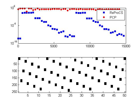
Figure 4: Comparison of ReProCS and PCP for the RPCA problem. The top plot is the relative error $\|\bm{\ell}_{t}-\hat{\bm{\ell}}_{t}\|_{2}/\|\bm{\ell}_{t}\|_{2}$. The bottom plot shows the sparsity pattern of $\bm{S}$ (black represents a non-zero entry). Results are averaged over 100 simulations and plotted every 300 time instants.

IX Extensions

In this section, we first give other models on changes in $\mathcal{T}_{t}$ that are special cases of the general model Model 5.1 and hence can also be used in Theorem 2.5 or 2.7. The next three subsections discuss various other results that can also be proved using the proof techniques developed in this work.

IX-A Other Models on Changes in $\mathcal{T}_{t}$

We give here other models on changes in $\mathcal{T}_{t}$ that are special cases of Model 5.1.

Model 9.1.

Suppose that $\mathcal{T}_{t}$ consists of consecutive indices and is of size $s$ or less, i.e. $|\mathcal{T}_{t}|\leq s$. When $\mathcal{T}_{t}$ is not empty, let $\tilde{o}_{t}$ denote its smallest (topmost) index. Let $\rho_{1}$ be an integer. We assume that $\tilde{o}_{t}$ satisfies the following Bernoulli-Gaussian model:

$$\tilde{o}_{t}=\lceil o_{t}\mod n\rceil\text{ where }o_{t}=o_{t-1}+\theta_{t}\left(1.1\frac{s}{\rho}+\varpi_{t}\right)$$

where $\varpi_{t}\sim\mathcal{N}(0,\sigma^{2})$ (Gaussian) and $\theta_{t}\sim Bernoulli(q)$. Assume that $\{\varpi_{t}\}$, $\{\theta_{t}\}$ are mutually independent and independent of $\bm{\ell}_{t}$’s. Taking the mod with respect to $n$ describes the process of the set $\mathcal{T}_{t}$ starting over at $1$ when its topmost index exceeds $n$ (this models a new object appearing after the old one has disappeared; notice that at any $t$ $\mathcal{T}_{t}$ could be empty as well, i.e. there may be no object).

Assume that $s\leq\frac{1.2\rho n}{\alpha}$, $q\geq 1-(\frac{n^{-10}}{2t_{\max}})^{\frac{1}{\beta}}$ for a $\beta$ that satisfies $\rho^{2}\frac{\beta}{\alpha}\leq 0.01$, and $\sigma^{2}\leq\frac{s^{2}}{4000\rho^{2}\log(n)}$.

Model 9.2.

Suppose that $\mathcal{T}_{t}$ consists of $s$ consecutive indices and suppose that it moves down the vector by between 1 and $m$ indices at every time $t$. When it reaches the bottom of the vector, we assume that it starts over at $1$. Assume that $s\leq 0.0025\alpha$ and $m\leq\frac{n-s}{\alpha}$.

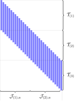
Figure 5: Model 9.2

Model 9.3.

In both models above we let $\mathcal{T}_{t}$ contain consecutive indices. This models a moving 1D object of length s or less that enters the scene and eventually walks out, and then another object of length $s$ or less may come in. However notice that nothing in our general model, Model 5.1, requires the indices to be consecutive or contiguous in any way. Thus in both of Models 9.1 and 9.2 above, instead of one moving object, we can also have multiple moving objects as long as the union of their supports is of size at most $s$ and satisfies one of these models. Also, with minor changes, the object(s) instead of leaving the scene can reflect back up and start moving in the other direction as well.

Lemma 9.4.

If $t_{\max}\leq n^{10}$, then Model 9.1 is a special case of Model 2.3 (and hence a special case of Model 5.1) with probability at least $1-n^{-10}$.

Proof.

The proof has three steps. (a) We first use standard arguments about a Bernoulli sequence [25] to prove that the object moves at least once every $\beta$ time instants with probability at least $1-0.5n^{-10}$. The choice of $q$ ensures that this holds. (b) Next we use a standard Gaussian tail bound argument to show that, with probability at least $1-0.5n^{-10}$, when it moves, it moves by at least $s/\rho$ indices and at most $1.2s/\rho$ indices. The bound on $\sigma^{2}$ ensures this. (c) The above two claims ensure that, w.h.p., the object remains static for at most $\beta$ frames at a time and when it moves it moves by at least $s/\rho$ indices and at most $1.2s/\rho$ indices. Notice that all the motion is in one direction. Motion by at least $s/\rho$ in one direction ensures that after the object moves $\rho$ times, i.e. after $\rho$ changes of $\mathcal{T}_{t}$, the sets are disjoint, i.e. $\mathcal{T}^{[k]}\cap\mathcal{T}^{[k+\rho]}=\emptyset$. Motion by at most $1.2s/\rho$ in one direction and $1.2\frac{s}{\rho}\alpha\leq n$ ensures the third condition of Model 2.3 holds even when the object moves at every frame. ∎

Lemma 9.5.

Model 9.2 is a special case of Model 5.1 with $\rho=2$ and $h^{+}=s/\alpha$.

See Figure 5 for a diagram of the model and the idea behind its proof.

Proof.

For the sake of clarity, we will prove the case when the object moves exactly 1 index at every time $t$. The only difference in the general case is the construction of the $\mathcal{J}_{(i),u}$.

Consider an interval $\mathcal{J}_{u}$. Let $t_{u}:=(u-1)\alpha+1$ denote the first time in $\mathcal{J}_{u}$. Without loss of generality (because we can re-label the indices) let the object start at the top of the vector. That is $\mathcal{T}_{t_{u}}=[1,s]$. Let $l_{u}=\left\lceil\frac{n}{s}\right\rceil$. Let $\mathcal{T}_{(i),u}=[(i-1)s+1,is]$ for $i=1,2,\dots,\left\lfloor\frac{n}{s}\right\rfloor$. If $\frac{n}{s}$ is not an integer, also define $\mathcal{T}_{\left(\left\lceil\frac{n}{s}\right\rceil\right),u}=\left[\left\lfloor\frac{n}{s}\right\rfloor s+1,n\right]$. Define $\mathcal{J}_{(i),u}:=[t_{u}+(i-1)s,t_{u}+is-1]$ for $i=1,2,\dots,\left\lfloor\frac{\alpha}{s}\right\rfloor$. If $\frac{\alpha}{s}$ is not an integer, also define $\mathcal{J}_{\left(\left\lceil\frac{\alpha}{s}\right\rceil\right),u}=[t_{u}+\left\lfloor\frac{\alpha}{s}\right\rfloor s,t_{u}+\alpha-1]$.

Clearly $\mathcal{J}_{(i),u}$ as defined above are a partition of $\mathcal{J}_{u}$. Also, by construction, for all $t\in\mathcal{J}_{(i),u}$, $\mathcal{T}_{t}\subseteq\mathcal{T}_{(i),u}\cup\mathcal{T}_{(i+1),u}$. This follows from three facts 1) the assumption that $\mathcal{T}_{t_{u}}=[1,s]$ (which is just a renumbering of the indices to make the numbers clearer) 2) the object moves down by exactly one index at each time $t$ and 3) $m\leq\frac{n-s}{\alpha}$, so that once an index leaves $\mathcal{T}_{t}$, it will not return in the next $\alpha$ time instants. A simpler way of stating fact 3) is that the total motion is such that $\mathcal{T}_{t}$ does not return to where it started i.e. $\mathcal{T}_{t_{u}}\cap\mathcal{T}_{t_{u}+\alpha}=\emptyset$.

Notice that $|\mathcal{J}_{(i),u}|\leq s$ for all $i$. (With the possible exception of the last set, they all have size exactly $s$.) So under the assumptions of Model 9.2 $h_{u}^{*}(\alpha)\leq s$, which satisfies Model 5.1 with $h^{+}=\frac{s}{\alpha}\leq 0.0025\alpha=\frac{0.01\alpha}{2^{2}}=\frac{0.01\alpha}{\rho^{2}}$. ∎

IX-B Analyze the ReProCS algorithm that also removes the deleted directions from the subspace estimate

The tools introduced in this paper – (a) Lemma 5.3 and the way it is applied to bound $\bm{\mathcal{H}}_{u}$ in Lemma 6.23; and (b) the detection lemma (Lemma 6.17), the no false detection lemma (Lemma 6.16) and the p-PCA lemma (Lemma 6.18) – can also be used to get a correctness result for a practical modification of ReProCS with cluster-PCA (ReProCS-cPCA) which is Algorithm 2 of [12]. This algorithm was introduced to also remove the deleted directions from the subspace estimate. It does this by re-estimating the previous subspace at a time after the newly added subspace has been accurately estimated (i.e. at a time after ${\hat{t}}_{j}+K\alpha$). A partial result for this algorithm was proved in [12].

This result will need one extra assumption – it will need the eigenvalues of the covariance matrix of $\bm{\ell}_{t}$ to be clustered for a period of time after the subspace change has stabilized, i.e. for a period of $d_{2}$ frames in the interval $[t_{j}+d+1,t_{j+1}-1]$ – but it will have a key advantage. It will need a much weaker denseness assumption and hence a much weaker bound on $r$ or $r_{\text{mat}}$. In particular, with this result we expect to be able to allow $r=r_{\text{mat}}\in\mathcal{O}(n)$ with the same assumptions on $s$ and $s_{\text{mat}}$ that we currently allow. This requirement is almost as weak as that of PCP.

IX-C Relax the independence assumption on $\ell_{t}$’s

The results in this work assume that the $\bm{\ell}_{t}$’s are independent over time and zero mean; this is a valid model when background images have independent random variations about a fixed mean. Using the tools developed in this paper, a similar result can also be obtained for the more general case of $\bm{\ell}_{t}$’s following an autoregressive model. This will allow the $\bm{\ell}_{t}$’s to be correlated over time. A partial result for this case was obtained in [zhan_reprocs]. The main change in this case will be that we will need to apply the matrix Azuma inequality from [23] instead of matrix Hoeffding. This is will also require algebraic manipulation of sums and some other important modifications, as explained in [zhan_reprocs], so that the constant term after conditioning on past values of the matrix is small.

IX-D Noisy and Undersampled Online Matrix Completion or Online Robust PCA

We expect that the tools introduced in this paper can also be used to analyze the noisy case, i.e. the case of $\bm{m}_{t}=\bm{x}_{t}+\bm{\ell}_{t}+\bm{w}_{t}$ where $\bm{w}_{t}$ is small bounded noise. In most practical video applications, while the foreground is truly sparse, the background is only approximately low-rank. The modeling error can be handled as $\bm{w}_{t}$. The proposed algorithms already apply without modification to this case (see [17] for results on real videos). The reason that our tools will directly extend to the noisy case is this: the sparse recovery step is already a noisy sparse recovery one, its analysis will not change if we also add in more noise due to $\bm{w}_{t}$. If $\bm{\ell}_{t}$ and $\bm{w}_{t}$ are assumed independent, then there should be few simple modifications to the analysis of the p-PCA step as well.

Finally, we expect both the algorithm and the proof techniques to apply with simple changes to the undersampled case $\bm{m}_{t}=\bm{A}_{t}\bm{x}_{t}+\bm{B}_{t}\bm{\ell}_{t}+\bm{w}_{t}$ as long as $\bm{B}_{t}$ is not time-varying, i.e. $\bm{B}_{t}=\bm{B}_{0}$. A partial result for this case was obtained in [26] and experiments were shown in [17].

X Conclusions

In this work, we obtained correctness results for online robust PCA and for online matrix completion. Both results needed four key assumptions: (a) accurate initial subspace knowledge; (b) slow subspace change and mutual independence of the $\bm{\ell}_{t}$’s according to Model 2.2; (c) some changes in the set of missing entries (or in the set of outlier-corrupted entries) over time, one way to quantify what is needed is given in Model 2.3; (d) a denseness assumption on the columns of the subspace basis matrices of $\bm{\ell}_{t}$; and (e) algorithm parameters are appropriately set.

Ongoing work includes obtaining the results mentioned in Sections IX-B, IX-C and IX-D. Besides these, we expect the proof techniques developed here to apply to various other problems involving PCA with data and noise terms being correlated.

Appendix A Proof that Model 2.3 on $\mathcal{T}_{t}$ satisfies the general Model 5.1

Proof of Lemma 5.2.

Consider an interval $\mathcal{J}_{u}$. We will construct one set of mutually disjoints sets $\{\mathcal{T}_{(i),u}\}_{i=1,2,\dots l_{u}}$ that are subsets of $\{1,2,\dots n\}$ and a partition $\{\mathcal{J}_{(i),u}\}_{i=1,2,\dots l_{u}}$ of $\mathcal{J}_{u}$ so that for all $t\in\mathcal{J}_{(i),u}$, (10) holds and so that $h_{u}(\alpha;\{\mathcal{T}_{(i),u}\},\{\mathcal{J}_{(i),u}\})\leq\beta$ for this choice. Since $h_{u}^{*}(\alpha)$ takes the minimum over all such sets, this will imply $h_{u}^{*}(\alpha)\leq\beta$. By setting $h^{+}=\beta/\alpha$ and using the Model 2.3 assumption ${\rho}^{2}\beta\leq 0.01\alpha$, we will be done.

Recall from Model 2.3 that $\mathcal{T}_{t}=\mathcal{T}^{[k]}$ for all $t\in[t^{k},t^{k+1})$ with $t^{k+1}-t^{k}<\beta$ and $|\mathcal{T}^{[k]}|\leq s$.

Let $t_{u}:=(u-1)\alpha+1$ denote the first time index of $\mathcal{J}_{u}$. Let $k_{u}$ be the index $k$ for which $t_{u}\in[t^{k},t^{k+1})$. In other words, $\mathcal{T}_{t_{u}}=\mathcal{T}^{[k_{u}]}$. Define $l_{u}$ to be the number of intervals $[t^{k},t^{k+1})$ that have non-empty intersection with $\mathcal{J}_{u}$. So $l_{u}$ is one plus the number of times $\mathcal{T}_{t}$ changes in the interval $\mathcal{J}_{u}$. For $i=1,2,\dots l_{u}-1$, define

$$\mathcal{T}_{(i),u}:=\mathcal{T}^{[k_{u}+i-1]}\setminus\mathcal{T}^{[k_{u}+i]},$$

and set $\mathcal{T}_{(l_{u}),u}=\mathcal{T}^{[k_{u}+l_{u}-1]}$. Clearly $l_{u}\leq\alpha$. Thus, by the Model 2.3 assumption (for any $k$ and $i$ such that $k<i\leq k+\alpha$, $(\mathcal{T}^{[k]}\setminus\mathcal{T}^{[k+1]})\cap(\mathcal{T}^{[i]}\setminus\mathcal{T}^{[i+1]})=\emptyset$), the $\mathcal{T}_{(i),u}$’s are mutually disjoint.

Next, define a partition of $\mathcal{J}_{u}$ as

$$\mathcal{J}_{(i),u}:=[t^{k_{u}+i-1},t^{k_{u}+i})\cap\mathcal{J}_{u}\ \text{for}\ i=1,2,\dots l_{u}$$

By Model 2.3 $1\leq t_{k+1}-t_{k}<\beta$ for all $k$. Since $\mathcal{J}_{(i),u}\subseteq[t^{k_{u}+i-1},t^{k_{u}+i})$, $|\mathcal{J}_{(i),u}|<\beta$ for all $i=1,2,\dots l_{u}$.

Notice that for all $t\in\mathcal{J}_{(i),u}$, $\mathcal{T}_{t}=\mathcal{T}^{[k_{u}+i-1]}$. So if we can show that $\mathcal{T}^{[k_{u}+i-1]}\subseteq\mathcal{T}_{(i),u}\cup\mathcal{T}_{(i+1),u}\dots\cup\mathcal{T}_{(i+\rho-1),u}$ for all $i=1,2,\dots l_{u}$, we will be done since this will imply $h_{u}^{*}(\alpha)\leq\beta$. To show this, set $k=k_{u}+i-1$. Then,

$$\mathcal{T}^{[k]} =\mathcal{T}_{(i),u}\cup[\mathcal{T}^{[k]}\cap\mathcal{T}^{[k+1]}]$$

$$=\mathcal{T}_{(i),u}\cup[\mathcal{T}^{[k]}\cap\mathcal{T}^{[k+1]}\setminus\mathcal{T}^{[k+2]}]\cup[\mathcal{T}^{[k]}\cap\mathcal{T}^{[k+1]}\cap\mathcal{T}^{[k+2]}]$$

$$\subseteq\mathcal{T}_{(i),u}\cup\mathcal{T}_{(i+1),u}\cup[\mathcal{T}^{[k]}\cap\mathcal{T}^{[k+1]}\cap\mathcal{T}^{[k+2]}]$$

$$=\mathcal{T}_{(i),u}\cup\mathcal{T}_{(i+1),u}\cup[\mathcal{T}^{[k]}\cap\mathcal{T}^{[k+1]}\cap\mathcal{T}^{[k+2]}\setminus\mathcal{T}^{[k+3]})\cup[\mathcal{T}^{[k]}\cap\mathcal{T}^{[k+1]}\cap\mathcal{T}^{[k+2]}\cap\mathcal{T}^{[k+3]}]$$

$$\subseteq\mathcal{T}_{(i),u}\cup\mathcal{T}_{(i+1),u}\cup\mathcal{T}_{(i+2)}\cup[\mathcal{T}^{[k]}\cap\mathcal{T}^{[k+1]}\cap\mathcal{T}^{[k+2]}\cap\mathcal{T}^{[k+3]}].$$

Continuing in the same manner as above, we get,

$$\mathcal{T}^{[k]} \subseteq \mathcal{T}_{(i),u}\cup\mathcal{T}_{(i+1),u}\cup\dots\cup\mathcal{T}_{(i+\rho-1),u}\cup[\mathcal{T}^{[k]}\cap\mathcal{T}^{[k+1]}\cap\dots\cap\mathcal{T}^{[k+\rho]}]$$ (30)

$$= \mathcal{T}_{(i),u}\cup\mathcal{T}_{(i+1),u}\cup\dots\cup\mathcal{T}_{(i+\rho-1),u}$$

The last line is because $\mathcal{T}^{[k]}\cap\mathcal{T}^{[k+\rho]}=\emptyset$ by Model 2.3. ∎

Appendix B Proof of Lemma 6.14 (bound on $\zeta_{j,\mathrm{new},k}^{+}$zeta j new k plus) and of Lemma 7.8

Proof of Lemma 6.14.

This proof’s approach is similar to that of [12, Lemma 6.1]. The details have some differences because our main result now uses different assumptions.

This lemma uses Model 5.1. As shown in Lemma 5.2, Model 2.3 is a special case of this general model.

Recall that $\displaystyle\zeta_{j,\mathrm{new},k}^{+}:=\frac{b_{\bm{\mathcal{H}},k}}{b_{\bm{A}}-b_{\bm{A},\perp}-b_{\bm{\mathcal{H}},k}}$ with the terms on the RHS defined in Lemmas 6.21, 6.22, 6.23.

Recall that $\epsilon=0.01r_{\mathrm{new}}\zeta{\hat{\lambda}_{\mathrm{train}}^{-}}$. Divide the numerator and denominator by ${\hat{\lambda}_{\mathrm{train}}^{-}}$. Define

$$B_{k}:=\begin{cases}\begin{array}[]{l}\left[\rho^{2}h^{+}(\phi^{+})^{2}(\kappa_{s}^{+})^{2}(\zeta_{j,\mathrm{new},k-1}^{+})+2\kappa_{s}^{+}\phi^{+}\right]\left(\frac{\lambda_{\mathrm{new}}^{+}}{{\hat{\lambda}_{\mathrm{train}}^{-}}}\right)\end{array}&k=1\\ \vspace{-.2in}\\ \begin{array}[]{l}\left[\rho^{2}h^{+}(\phi^{+})^{2}\zeta_{j,\mathrm{new},k-1}^{+}+2\sqrt{\rho^{2}h^{+}}\phi^{+}\right]\left(\frac{\lambda_{\mathrm{new}}^{+}}{{\hat{\lambda}_{\mathrm{train}}^{-}}}\right)\end{array}&k\geq 2\end{cases}$$

$$C_{k}:=\left[\rho^{2}h^{+}(\phi^{+})^{2}(\zeta_{j,*}^{+})r+2\sqrt{\rho^{2}h^{+}}\phi^{+}(\zeta_{j,*}^{+})r+2(\zeta_{j,*}^{+})r\right]\left(\frac{\lambda^{+}}{{\hat{\lambda}_{\mathrm{train}}^{-}}}\right)+0.05$$

$$D_{k}:= 1-(\zeta_{j,*}^{+})^{2}-(\zeta_{j,*}^{+})^{2}\left(\frac{\lambda^{+}}{{\hat{\lambda}_{\mathrm{train}}^{-}}}\right)-\zeta_{j,\mathrm{new},k-1}^{+}B_{k}-r_{\mathrm{new}}\zeta(C_{k}+.02)$$

Then,

$$\zeta_{j,\mathrm{new},k}^{+}\leq\zeta_{j,\mathrm{new},k-1}^{+}\frac{B_{k}}{D_{k}}+r_{\mathrm{new}}\zeta\frac{C_{k}}{D_{k}}.$$

Recall that $\kappa_{s}^{+}=0.0215$ and $\phi^{+}=1.2$. It is not difficult to see that $\zeta_{j,\mathrm{new},k}^{+}$ is an increasing function of $\rho^{2}h^{+}$, $r$, $\zeta$, $\zeta\frac{\lambda^{+}}{{\hat{\lambda}_{\mathrm{train}}^{-}}}$, and $\frac{\lambda_{\mathrm{new}}^{+}}{{\hat{\lambda}_{\mathrm{train}}^{-}}}$ and $\zeta_{j,\mathrm{new},k-1}^{+}$. Consider $k=1$. Using $\zeta_{j,\mathrm{new},0}^{+}=1$ and the upper bounds assumed in Theorem 2.7 on the above quantities, we get that $\zeta_{j,\mathrm{new},1}^{+}\leq 0.18$.

Thus, $\zeta_{j,\mathrm{new},1}^{+}\leq\zeta_{j,\mathrm{new},0}^{+}=1$. Using this and the fact that $\zeta_{j,\mathrm{new},k}^{+}$ is an increasing function of $\zeta_{j,\mathrm{new},k-1}^{+}$, we can show by induction that $\zeta_{j,\mathrm{new},k}^{+}\leq\zeta_{j,\mathrm{new},k-1}^{+}$. Thus, $\zeta_{j,\mathrm{new},k}^{+}\leq\zeta_{j,\mathrm{new},1}^{+}\leq 0.18$ for all $k=1,2\dots K$.

Using $\zeta_{j,\mathrm{new},k}^{+}\leq 0.18$ and the bounds assumed in Theorem 2.7 on the other quantities we get that

$$\zeta_{j,\mathrm{new},k}^{+}\leq 0.83\zeta_{j,\mathrm{new},k-1}^{+}+0.14r_{\mathrm{new}}\zeta$$

Using this, we get

$$\zeta_{j,\mathrm{new},k}^{+}\leq 0.83\zeta_{j,\mathrm{new},k-1}^{+}+0.14r_{\mathrm{new}}\zeta \leq\zeta_{j,\mathrm{new},0}^{+}(0.83)^{k}+\sum_{i=0}^{k-1}(0.83)^{i}(0.14)r_{\mathrm{new}}\zeta$$

$$\leq\zeta_{j,\mathrm{new},0}^{+}(0.83)^{k}+\sum_{i=0}^{\infty}(0.83)^{i}(0.14)r_{\mathrm{new}}\zeta$$

$$\leq 0.83^{k}+0.84r_{\mathrm{new}}\zeta.$$

∎

Proof of Lemma 7.8.

Recall that $\bm{D}_{j,\mathrm{new}}=(\bm{I}-\hat{\bm{P}}_{(j),*}\hat{\bm{P}}_{(j),*}{}^{\prime})\bm{P}_{(j),\mathrm{new}}$. Then $\|{\bm{I}_{\mathcal{T}}}^{\prime}\bm{D}_{j,\mathrm{new}}\|_{2}=\|{\bm{I}_{\mathcal{T}}}^{\prime}(\bm{I}-\hat{\bm{P}}_{(j),*}\hat{\bm{P}}_{(j),*}{}^{\prime})\bm{P}_{(j),\mathrm{new}}\|_{2}\leq\|{\bm{I}_{\mathcal{T}}}^{\prime}\bm{P}_{(j),\mathrm{new}}\|_{2}+\|\hat{\bm{P}}_{(j),*}{}^{\prime}\bm{P}_{(j),\mathrm{new}}\|_{2}\leq\kappa_{s}(\bm{P}_{(j),\mathrm{new}})+\|\hat{\bm{P}}_{(j),*}{}^{\prime}(\bm{I}-\bm{P}_{(j),*}{\bm{P}_{(j),*}}^{\prime})\bm{P}_{(j),\mathrm{new}}\|_{2}\leq\kappa_{s}(\bm{P}_{(j),\mathrm{new}})+\zeta_{j,*}$. The event $X_{\hat{u}_{j}+k-1}\in\Gamma_{j,k-1}^{\hat{u}_{j}}$ implies that $\zeta_{j,*}\leq\zeta_{j,*}^{+}\leq 0.0015$. Thus, the lemma follows. ∎

Appendix C Proof of the Compressed Sensing (CS) Lemma (Lemma 6.15)

This proof’s approach is similar to that of [12, Lemma 6.4]. The details have some differences because our main result now uses different assumptions. The proof uses the denseness assumption and subspace error bounds $\zeta_{j,*}\leq\zeta_{j,*}^{+}$ and $\zeta_{j,\mathrm{new},k-1}\leq\zeta_{j,\mathrm{new},k-1}^{+}$, that hold when $X_{\hat{u}_{j}+k-1}\in\Gamma_{j,k-1}^{\hat{u}_{j}}$ for $\hat{u}_{j}=u_{j}$ or $\hat{u}_{j}=u_{j}+1$, to obtain bounds on the restricted isometry constant (RIC) of the sparse recovery matrix $\bm{\Phi}_{t}$ and the sparse recovery error $\|\bm{b}_{t}\|_{2}$. Applying the noisy compressed sensing (CS) result from [19] and the assumed bounds on $\zeta$ and $\gamma$, the lemma follows.

Lemma C.1.

[12, Lemma 2.10] Suppose that $\bm{P}$, $\hat{\bm{P}}$ and $\bm{Q}$ are three basis matrices. Also, $\bm{P}$ and $\hat{\bm{P}}$ are of the same size, $\bm{Q}^{\prime}\bm{P}=\bm{0}$ and $\|(\bm{I}-\hat{\bm{P}}\hat{\bm{P}}{}^{\prime})\bm{P}\|_{2}=\zeta_{*}$. Then,

1. $\|(\bm{I}-\hat{\bm{P}}\hat{\bm{P}}{}^{\prime})\bm{P}\bm{P}^{\prime}\|_{2}=\|(\bm{I}-\bm{P}\bm{P}^{\prime})\hat{\bm{P}}\hat{\bm{P}}{}^{\prime}\|_{2}=\|(\bm{I}-\bm{P}\bm{P}^{\prime})\hat{\bm{P}}\|_{2}=\|(\bm{I}-\hat{\bm{P}}\hat{\bm{P}}{}^{\prime})\bm{P}\|_{2}=\zeta_{*}$

2. $\|\bm{P}\bm{P}^{\prime}-\hat{\bm{P}}\hat{\bm{P}}{}^{\prime}\|_{2}\leq 2\|(\bm{I}-\hat{\bm{P}}\hat{\bm{P}}{}^{\prime})\bm{P}\|_{2}=2\zeta_{*}$

3. $\|\hat{\bm{P}}{}^{\prime}\bm{Q}\|_{2}\leq\zeta_{*}$

4. $\sqrt{1-\zeta_{*}^{2}}\leq\sigma_{i}\left((\bm{I}-\hat{\bm{P}}\hat{\bm{P}}{}^{\prime})\bm{Q}\right)\leq 1$

We begin by first bounding the RIC of the CS matrix $\bm{\Phi}_{t}$. We will use the notation $\kappa_{s}^{2}(\bm{P})$ to mean $\left(\kappa_{s}(\bm{P})\right)^{2}$.

Lemma C.2 (Bounding the RIC of $\bm{\Phi}_{t}$ [12, Lemma 6.6]).

Recall that $\zeta_{j,*}:=\|(\bm{I}-\hat{\bm{P}}_{(j),*}\hat{\bm{P}}_{(j),*}{}^{\prime})\bm{P}_{(j),*}\|_{2}$. The following hold.

1. Suppose that a basis matrix $\bm{P}$ can be split as $\bm{P}=[\bm{P}_{1}\ \bm{P}_{2}]$ where $\bm{P}_{1}$ and $\bm{P}_{2}$ are also basis matrices. Then $\kappa_{s}^{2}(\bm{P})=\max_{\mathcal{T}:|\mathcal{T}|\leq s}\|{\bm{I}_{\mathcal{T}}}^{\prime}\bm{P}\|_{2}^{2}\leq\kappa_{s}^{2}(\bm{P}_{1})+\kappa_{s}^{2}(\bm{P}_{2})$.

2. $\kappa_{s}^{2}(\hat{\bm{P}}_{(j),*})\leq(\kappa_{s,*})^{2}+2\zeta_{*}$ for all $j$

3. $\kappa_{s}(\hat{\bm{P}}_{(j),\mathrm{new},k})\leq\kappa_{s,\mathrm{new}}+\zeta_{j,\mathrm{new},k}+\zeta_{j,*}$ for all $j$ and $k$.

4. For $t\in[(u_{j-1}+K)\alpha+1,(\hat{u}_{j}+1)\alpha)$, $\delta_{s}(\bm{\Phi}_{t})=\kappa_{s}^{2}(\hat{\bm{P}}_{(j),*})\leq(\kappa_{s,*})^{2}+2\zeta_{j,*}$.

5. For $k=1,\dots,K-1$, for $t\in[(\hat{u}_{j}+k)\alpha+1,(\hat{u}_{j}+k+1)\alpha]$ $\delta_{s}(\bm{\Phi}_{t})=\kappa_{s}^{2}([\hat{\bm{P}}_{(j),*}\ \hat{\bm{P}}_{(j),\mathrm{new},k}])\leq\kappa_{s}^{2}(\hat{\bm{P}}_{(j),*})+\kappa_{s}^{2}(\hat{\bm{P}}_{(j),\mathrm{new},k})\leq(\kappa_{s,*})^{2}+2\zeta_{j,*}+(\kappa_{s,\mathrm{new}}+\zeta_{j,\mathrm{new},k}+\zeta_{j,*})^{2}$.

Proof.

1. Recall that $\kappa_{s}^{2}(\bm{P})=\max_{|\mathcal{T}|\leq s}\|{\bm{I}_{\mathcal{T}}}^{\prime}\bm{P}\|_{2}^{2}$. Also, $\|{\bm{I}_{\mathcal{T}}}^{\prime}\bm{P}\|_{2}^{2}=\|{\bm{I}_{\mathcal{T}}}^{\prime}[\bm{P}_{1}\ \bm{P}_{2}][\bm{P}_{1}\ \bm{P}_{2}]^{\prime}\bm{I}_{\mathcal{T}}\|_{2}=\|{\bm{I}_{\mathcal{T}}}^{\prime}(\bm{P}_{1}{\bm{P}_{1}}^{\prime}+\bm{P}_{2}{\bm{P}_{2}}^{\prime})\bm{I}_{\mathcal{T}}\|_{2}\leq\|{\bm{I}_{\mathcal{T}}}^{\prime}\bm{P}_{1}{\bm{P}_{1}}^{\prime}\bm{I}_{\mathcal{T}}\|_{2}+\|{\bm{I}_{\mathcal{T}}}^{\prime}\bm{P}_{2}{\bm{P}_{2}}^{\prime}\bm{I}_{\mathcal{T}}\|_{2}$. Thus, the inequality follows.

2. For any set $\mathcal{T}$ with $|\mathcal{T}|\leq s$, $\|{\bm{I}_{\mathcal{T}}}^{\prime}\hat{\bm{P}}_{(j),*}\|_{2}^{2}=\|{\bm{I}_{\mathcal{T}}}^{\prime}\hat{\bm{P}}_{(j),*}\hat{\bm{P}}_{(j),*}{}^{\prime}\bm{I}_{\mathcal{T}}\|_{2}=\|{\bm{I}_{\mathcal{T}}}^{\prime}(\hat{\bm{P}}_{(j),*}\hat{\bm{P}}_{(j),*}{}^{\prime}-\bm{P}_{(j),*}{\bm{P}_{(j),*}}^{\prime}+\bm{P}_{(j),*}{\bm{P}_{(j),*}}^{\prime})\bm{I}_{\mathcal{T}}\|_{2}\leq\|{\bm{I}_{\mathcal{T}}}^{\prime}(\hat{\bm{P}}_{(j),*}\hat{\bm{P}}_{(j),*}{}^{\prime}-\bm{P}_{(j),*}{\bm{P}_{(j),*}}^{\prime})\bm{I}_{\mathcal{T}}\|_{2}+\|{\bm{I}_{\mathcal{T}}}^{\prime}\bm{P}_{(j),*}{\bm{P}_{(j),*}}^{\prime}\bm{I}_{\mathcal{T}}\|_{2}\leq 2\zeta_{j,*}+(\kappa_{s,*})^{2}$. The last inequality follows using Lemma C.1 with $\bm{P}=\bm{P}_{(j),*}$ and $\hat{\bm{P}}=\hat{\bm{P}}_{(j),*}$.

3. By Lemma C.1 with $\bm{P}=\bm{P}_{(j),*}$, $\hat{\bm{P}}=\hat{\bm{P}}_{(j),*}$ and $\bm{Q}=\bm{P}_{(j),\mathrm{new}}$, $\|{\bm{P}_{(j),\mathrm{new}}}^{\prime}\hat{\bm{P}}_{(j),*}\|_{2}\leq\zeta_{j,*}$. By Lemma C.1 with $\bm{P}=\bm{P}_{(j),\mathrm{new}}$ and $\hat{\bm{P}}=\hat{\bm{P}}_{(j),\mathrm{new},k}$, $\|(\bm{I}-\bm{P}_{(j),\mathrm{new}}{\bm{P}_{(j),\mathrm{new}}}^{\prime})\hat{\bm{P}}_{(j),\mathrm{new},k}\|_{2}=\|(\bm{I}-\hat{\bm{P}}_{(j),\mathrm{new},k}\hat{\bm{P}}_{(j),\mathrm{new},k}{}^{\prime})\bm{P}_{(j),\mathrm{new}}\|_{2}$.

   For any set $\mathcal{T}$ with $|\mathcal{T}|\leq s$, $\|{\bm{I}_{\mathcal{T}}}^{\prime}\hat{\bm{P}}_{(j),\mathrm{new},k}\|_{2}\leq\|{\bm{I}_{\mathcal{T}}}^{\prime}(\bm{I}-\bm{P}_{(j),\mathrm{new}}{\bm{P}_{(j),\mathrm{new}}}^{\prime})\hat{\bm{P}}_{(j),\mathrm{new},k}\|_{2}+\|{\bm{I}_{\mathcal{T}}}^{\prime}\bm{P}_{(j),\mathrm{new}}{\bm{P}_{(j),\mathrm{new}}}^{\prime}\hat{\bm{P}}_{(j),\mathrm{new},k}\|_{2}\leq\|(\bm{I}-\bm{P}_{(j),\mathrm{new}}{\bm{P}_{(j),\mathrm{new}}}^{\prime})\hat{\bm{P}}_{(j),\mathrm{new},k}\|_{2}+\|{\bm{I}_{\mathcal{T}}}^{\prime}\bm{P}_{(j),\mathrm{new}}\|_{2}=\|(\bm{I}-\hat{\bm{P}}_{(j),\mathrm{new},k}\hat{\bm{P}}_{(j),\mathrm{new},k}{}^{\prime})\bm{P}_{(j),\mathrm{new}}\|_{2}+\|{\bm{I}_{\mathcal{T}}}^{\prime}\bm{P}_{(j),\mathrm{new}}\|_{2}\leq\|\bm{D}_{(j),\mathrm{new},k}\|_{2}+\|\hat{\bm{P}}_{(j),*}\hat{\bm{P}}_{(j),*}{}^{\prime}\bm{P}_{(j),\mathrm{new}}\|_{2}+\|{\bm{I}_{\mathcal{T}}}^{\prime}\bm{P}_{(j),\mathrm{new}}\|_{2}$. Taking $\max$ over $|\mathcal{T}|\leq s$ the claim follows.

4. This follows using Lemma 2.9 and the second claim of this lemma.

5. This follows using Lemma 2.9 and the first three claims of this lemma.

∎

Corollary C.3.

1. Conditioned on $\Gamma_{j-1,\mathrm{end}}$, for $t\in[t_{j},({\hat{u}}_{j}+1)\alpha]$, $\delta_{s}(\bm{\Phi}_{t})\leq\delta_{2s}(\bm{\Phi}_{t})\leq(\kappa_{2s,*})^{2}+2\zeta_{j,*}^{+}<0.1<0.1479$, and $\|[({\bm{\Phi}_{t})_{\mathcal{T}_{t}}}^{\prime}(\bm{\Phi}_{t})_{\mathcal{T}_{t}}]^{-1}\|_{2}\leq\frac{1}{1-\delta_{s}(\bm{\Phi}_{t})}<1.2:=\phi^{+}$.

2. For $k=2,\dots,K$ and $\hat{u}_{j}=u_{j}$ or $\hat{u}_{j}=u_{j}+1$, conditioned on $\Gamma_{j,k-1}^{\hat{u}_{j}}$, for $t\in[(\hat{u}_{j}+k-1)\alpha+1,(\hat{u}_{j}+k)\alpha]$, $\delta_{s}(\bm{\Phi}_{t})\leq\delta_{2s}(\bm{\Phi}_{t})\leq(\kappa_{2s,*})^{2}+2\zeta_{j,*}^{+}+(\kappa_{2s,\mathrm{new}}+\zeta_{j,\mathrm{new},k-1}^{+}+\zeta_{j,*}^{+})^{2}<0.1479$, and $\|[({\bm{\Phi}_{t})_{\mathcal{T}_{t}}}^{\prime}(\bm{\Phi}_{t})_{\mathcal{T}_{t}}]^{-1}\|_{2}\leq\frac{1}{1-\delta_{s}(\bm{\Phi}_{t})}<1.2:=\phi^{+}$.

3. For $\hat{u}_{j}=u_{j}$ or $\hat{u}_{j}=u_{j}+1$, conditioned on $\Gamma_{j,K}^{\hat{u}_{j}}$, for $t\in[(\hat{u}_{j}+K)\alpha+1,t_{j+1}-1]$, $\delta_{s}(\bm{\Phi}_{t})\leq\delta_{2s}(\bm{\Phi}_{t})\leq(\kappa_{2s,*})^{2}+2\zeta_{j,*}^{+}<0.1<0.1479$, and $\|[({\bm{\Phi}_{t})_{\mathcal{T}_{t}}}^{\prime}(\bm{\Phi}_{t})_{\mathcal{T}_{t}}]^{-1}\|_{2}\leq\frac{1}{1-\delta_{s}(\bm{\Phi}_{t})}<1.2:=\phi^{+}$.

Proof.

This follows using Lemma C.2, the definitions of $\Gamma_{j-1,\mathrm{end}}$ and $\Gamma_{j,k}^{\hat{u}_{j}}$, and the bound on $\zeta_{j,\mathrm{new},k-1}^{+}$ from Lemma 6.14. ∎

The following are straightforward bounds that will be useful for the proof of Lemma 6.15.

Fact C.4.

Under the assumptions of Theorem 2.7:

• $\zeta_{j,*}^{+}\gamma\leq\frac{\sqrt{\zeta}}{\sqrt{r_{0}+(J-1)c}}\leq\sqrt{\zeta}$

• $\zeta_{j,\mathrm{new},k-1}^{+}\leq 0.83^{k-1}+0.84r_{\mathrm{new}}\zeta$ (from Lemma 6.14)

• $\zeta_{j,\mathrm{new},k-1}^{+}\gamma_{\mathrm{new}}\leq 0.83^{k-1}\gamma_{\mathrm{new}}+0.84r_{\mathrm{new}}\zeta\gamma_{\mathrm{new}}\leq 0.83^{k-1}\gamma_{\mathrm{new}}+0.3\sqrt{\zeta}$

Proof of Lemma 6.15.

We will prove claim 2). The others are done in the same way.

Recall that $\Gamma_{j,k-1}^{\hat{u}_{j}}$ implies that $\zeta_{j,*}\leq\zeta_{j,*}^{+}$ and $\zeta_{j,\mathrm{new},k-1}\leq\zeta_{j,\mathrm{new},k-1}^{+}$.

1. For $t\in[({\hat{u}}_{j}+k-1)\alpha+1,(\hat{u}_{j}+k)\alpha]$, $\bm{b}_{t}:=(\bm{I}-\hat{\bm{P}}_{t-1}\hat{\bm{P}}_{t-1}{}^{\prime})\bm{\ell}_{t}=\bm{D}_{j,*,k-1}\bm{a}_{t,*}+\bm{D}_{j,\mathrm{new},k-1}\bm{a}_{t,\mathrm{new}}$. Thus, using Fact C.4

   $$\|\bm{b}_{t}\|_{2} \leq\zeta_{j,*}\sqrt{r}\gamma+\zeta_{j,\mathrm{new},k-1}\sqrt{r_{\mathrm{new}}}\gamma_{\mathrm{new}}$$

   $$\leq\sqrt{\zeta}\sqrt{r}+(0.83^{k-1}\gamma_{\mathrm{new}}+0.84\sqrt{\zeta})\sqrt{r_{\mathrm{new}}}$$

   $$=\sqrt{r_{\mathrm{new}}}0.83^{k-1}\gamma_{\mathrm{new}}+\sqrt{\zeta}(\sqrt{r}+0.84\sqrt{r_{\mathrm{new}}})\leq\xi.$$

2. By Corollary C.3, $\delta_{2s}(\bm{\Phi}_{t})<0.15<\sqrt{2}-1$. Given $|\mathcal{T}_{t}|\leq s$, $\|\bm{b}_{t}\|_{2}\leq\xi$, by the theorem in [19], the CS error satisfies

   $$\|\hat{\bm{x}}_{t,\text{cs}}-\bm{x}_{t}\|_{2}\leq\frac{4\sqrt{1+\delta_{2s}(\bm{\Phi}_{t})}}{1-(\sqrt{2}+1)\delta_{2s}(\bm{\Phi}_{t})}\xi<7\xi.$$

3. Using the above, $\|\hat{\bm{x}}_{t,\text{cs}}-\bm{x}_{t}\|_{\infty}\leq 7\xi$. Since $\min_{i\in\mathcal{T}_{t}}|(\bm{x}_{t})_{i}|\geq x_{\min}$ and $(\bm{x}_{t})_{\mathcal{T}_{t}^{c}}=0$, $\min_{i\in\mathcal{T}_{t}}|(\hat{\bm{x}}_{t,\text{cs}})_{i}|\geq x_{\min}-7\xi$ and $\max_{i\in\bar{\mathcal{T}_{t}}}|(\hat{\bm{x}}_{t,\text{cs}})_{i}|\leq 7\xi$. If $\omega<x_{\min}-7\xi$, then $\hat{\mathcal{T}}_{t}\supseteq\mathcal{T}_{t}$. On the other hand, if $\omega>7\xi$, then $\hat{\mathcal{T}}_{t}\subseteq\mathcal{T}_{t}$. Since $\omega$ satisfies $7\xi\leq\omega\leq x_{\min}-7\xi$, the support of $\bm{x}_{t}$ is exactly recovered, i.e. $\hat{\mathcal{T}}_{t}=\mathcal{T}_{t}$.

4. Given $\hat{\mathcal{T}}_{t}=\mathcal{T}_{t}$, the least squares estimate of $\bm{x}_{t}$ satisfies $(\hat{\bm{x}}_{t})_{\mathcal{T}_{t}}=[(\bm{\Phi}_{t})_{\mathcal{T}_{t}}]^{{\dagger}}\bm{y}_{t}=[(\bm{\Phi}_{t})_{\mathcal{T}_{t}}]^{{\dagger}}(\bm{\Phi}_{t}\bm{x}_{t}+\bm{\Phi}_{t}\bm{\ell}_{t})$ and $(\hat{\bm{x}}_{t})_{\bar{\mathcal{T}_{t}}}=\bm{0}$. Also, ${(\bm{\Phi}_{t})_{\mathcal{T}_{t}}}^{\prime}\bm{\Phi}_{t}={\bm{I}_{\mathcal{T}_{t}}}^{\prime}\bm{\Phi}_{t}$ (this follows since $(\bm{\Phi}_{t})_{\mathcal{T}_{t}}=\bm{\Phi}_{t}\bm{I}_{\mathcal{T}_{t}}$ and ${\bm{\Phi}_{t}}^{\prime}\bm{\Phi}_{t}=\bm{\Phi}_{t}$). Using this, the error $\bm{e}_{t}:=\hat{\bm{x}}_{t}-\bm{x}_{t}$ satisfies (18). Thus, using Fact C.4 and the bounds on $\|\bm{a}_{t}\|_{\infty}$ and $\|\bm{a}_{t,\mathrm{new}}\|_{\infty}$, for $t\in[({\hat{u}}_{j}+k-1)\alpha+1,(\hat{u}_{j}+k)\alpha]$,

   $$\|\bm{e}_{t}\|_{2} \leq\phi^{+}(\zeta_{j,*}^{+}\sqrt{r}\gamma+\zeta_{j,\mathrm{new},k-1}^{+}\sqrt{r_{\mathrm{new}}}\gamma_{\mathrm{new}})\leq 1.2\left(1.06\sqrt{\zeta}+(0.83)^{k-1}\sqrt{r_{\mathrm{new}}}\gamma_{\mathrm{new}}\right)$$

   The last inequality follows from Lemma 6.14.

∎

Appendix D Proof of Cauchy-Schwarz inequality for matrices

Lemma D.1 (Cauchy-Schwarz for a sum of vectors).

For vectors $\bm{x}_{t}$ and $\bm{y}_{t}$,

$$\left(\sum_{t=1}^{\alpha}{\bm{x}_{t}}^{\prime}\bm{y}_{t}\right)^{2}\leq\left(\sum_{t}\|\bm{x}_{t}\|_{2}^{2}\right)\left(\sum_{t}\|\bm{y}_{t}\|_{2}^{2}\right)$$

Proof.

$$\left(\sum_{t=1}^{\alpha}{\bm{x}_{t}}^{\prime}\bm{y}_{t}\right)^{2}=\left([{\bm{x}_{1}}^{\prime},\dots,{\bm{x}_{\alpha}}^{\prime}]\left[\begin{array}[]{c}\bm{y}_{1}\\ \vdots\\ \bm{y}_{\alpha}\end{array}\right]\right)^{2}\leq\left\|\left[\begin{array}[]{c}\bm{x}_{1}\\ \vdots\\ \bm{x}_{\alpha}\end{array}\right]\right\|_{2}^{2}\left\|\left[\begin{array}[]{c}\bm{y}_{1}\\ \vdots\\ \bm{y}_{\alpha}\end{array}\right]\right\|_{2}^{2}=\left(\sum_{t=1}^{\alpha}\|\bm{x}_{t}\|_{2}^{2}\right)\left(\sum_{t=1}^{\alpha}\|\bm{y}_{t}\|_{2}^{2}\right)$$

The inequality is by Cauchy-Schwarz for a single vector. ∎

Lemma D.2 (Cauchy-Schwarz for a sum of matrices).

For matrices $\bm{X}_{t}$ and $\bm{Y}_{t}$,

$$\left\|\frac{1}{\alpha}\sum_{t=1}^{\alpha}\bm{X}_{t}{\bm{Y}_{t}}^{\prime}\right\|_{2}^{2}\leq\lambda_{\max}\left(\frac{1}{\alpha}\sum_{t=1}^{\alpha}\bm{X}_{t}{\bm{X}_{t}}^{\prime}\right)\lambda_{\max}\left(\frac{1}{\alpha}\sum_{t=1}^{\alpha}\bm{Y}_{t}{\bm{Y}_{t}}^{\prime}\right)$$

Proof of Lemma D.2.

$$\left\|\sum_{t=1}^{\alpha}\bm{X}_{t}{\bm{Y}_{t}}^{\prime}\right\|_{2}^{2} =\max_{\begin{subarray}{c}\|\bm{x}\|=1\\ \|\bm{y}\|=1\end{subarray}}\left|\bm{x}^{\prime}\left(\sum_{t}\bm{X}_{t}{\bm{Y}_{t}}^{\prime}\right)\bm{y}\right|^{2}$$

$$=\max_{\begin{subarray}{c}\|\bm{x}\|=1\\ \|\bm{y}\|=1\end{subarray}}\left|\sum_{t=1}^{\alpha}({\bm{X}_{t}}^{\prime}\bm{x})^{\prime}({\bm{Y}_{t}}^{\prime}\bm{y})\right|^{2}$$

$$\leq\max_{\begin{subarray}{c}\|\bm{x}\|=1\\ \|\bm{y}\|=1\end{subarray}}\left(\sum_{t=1}^{\alpha}\left\|{\bm{X}_{t}}^{\prime}\bm{x}\right\|_{2}^{2}\right)\left(\sum_{t=1}^{\alpha}\left\|{\bm{Y}_{t}}^{\prime}\bm{y}\right\|_{2}^{2}\right)$$

$$=\max_{\|\bm{x}\|=1}\bm{x}^{\prime}\sum_{t=1}^{\alpha}\bm{X}_{t}{\bm{X}_{t}}^{\prime}\ \bm{x}\ \cdot\ \max_{\|\bm{y}\|=1}\bm{y}^{\prime}\sum_{t=1}^{\alpha}\bm{Y}_{t}{\bm{Y}_{t}}^{\prime}\ \bm{y}$$

$$=\lambda_{\max}\left(\sum_{t=1}^{\alpha}\bm{X}_{t}{\bm{X}_{t}}^{\prime}\right)\lambda_{\max}\left(\sum_{t=1}^{\alpha}\bm{Y}_{t}{\bm{Y}_{t}}^{\prime}\right)$$

The inequality is by Lemma D.1. The penultimate line is because $\|\bm{x}\|_{2}^{2}={\bm{x}^{\prime}\bm{x}}$. Multiplying both sides by $\left(\frac{1}{\alpha}\right)^{2}$ gives the desired result. ∎

References

- [1] B. Lois and N. Vaswani, “A correctness result for online robust pca,” in IEEE Intl. Conf. Acoustics, Speech, Sig. Proc. (ICASSP), 2015.
- [2] E. J. Candès, X. Li, Y. Ma, and J. Wright, “Robust principal component analysis?” Journal of ACM, vol. 58, no. 3, 2011.
- [3] V. Chandrasekaran, S. Sanghavi, P. A. Parrilo, and A. S. Willsky, “Rank-sparsity incoherence for matrix decomposition,” SIAM Journal on Optimization, vol. 21, 2011.
- [4] D. Hsu, S. Kakade, and T. Zhang, “Robust matrix decomposition with sparse corruptions,” IEEE Trans. Info. Th., Nov. 2011.
- [5] M. Fazel, “Matrix rank minimization with applications,” PhD thesis, Stanford University, 2002.
- [6] E. J. Candès and B. Recht, “Exact matrix completion via convex optimization,” Found. of Comput. Math, no. 9, pp. 717–772, 2008.
- [7] M. Brand, “Incremental singular value decomposition of uncertain data with missing values,” in Eur. Conf. on Comp. Vis. (ECCV), 2002.
- [8] L. Balzano, B. Recht, and R. Nowak, “Online Identification and Tracking of Subspaces from Highly Incomplete Information,” in Allerton Conf. Communication, Control, and Computing, 2010.
- [9] Y. Chi, Y. C. Eldar, and R. Calderbank, “Petrels: Parallel subspace estimation and tracking by recursive least squares from partial observations,” IEEE Trans. Sig. Proc., December 2013.
- [10] L. Balzano and S. Wright, “Local convergence of an algorithm for subspace identification from partial data,” arXiv:1306.3391 [cs.NA].
- [11] A. Krishnamurthy and A. Singh, “Low-rank matrix and tensor completion via adaptive sampling,” in Advances in Neural Information Processing Systems 26, C. Burges, L. Bottou, M. Welling, Z. Ghahramani, and K. Weinberger, Eds. Curran Associates, Inc., 2013, pp. 836–844. [Online]. Available: http://papers.nips.cc/paper/4954-low-rank-matrix-and-tensor-completion-via-adaptive-sampling.pdf
- [12] C. Qiu, N. Vaswani, B. Lois, and L. Hogben, “Recursive robust pca or recursive sparse recovery in large but structured noise,” IEEE Trans. Info. Th., Aug. 2014, shorter versions in ICASSP 2013 and ISIT 2013.
- [13] J. Feng, H. Xu, and S. Yan, “Online robust pca via stochastic optimization,” in Adv. Neural Info. Proc. Sys. (NIPS), 2013.
- [14] J. Feng, H. Xu, S. Mannor, and S. Yan, “Online pca for contaminated data,” in Advances in Neural Information Processing Systems 26, C. Burges, L. Bottou, M. Welling, Z. Ghahramani, and K. Weinberger, Eds. Curran Associates, Inc., 2013, pp. 764–772. [Online]. Available: http://papers.nips.cc/paper/5135-online-pca-for-contaminated-data.pdf
- [15] J. He, L. Balzano, and A. Szlam, “Incremental gradient on the grassmannian for online foreground and background separation in subsampled video,” in IEEE Conf. on Comp. Vis. Pat. Rec. (CVPR), 2012.
- [16] P. Netrapalli, P. Jain, and S. Sanghavi, “Low-rank matrix completion using alternating minimization,” in Symposium on Theory of Computing (STOC), 2013.
- [17] H. Guo, C. Qiu, and N. Vaswani, “An online algorithm for separating sparse and low-dimensional signal sequences from their sum,” IEEE Trans. Sig. Proc., Aug. 2014.
- [18] F. D. L. Torre and M. J. Black, “A framework for robust subspace learning,” International Journal of Computer Vision, vol. 54, pp. 117–142, 2003.
- [19] E. Candes, “The restricted isometry property and its implications for compressed sensing,” Compte Rendus de l’Academie des Sciences, Paris, Serie I, pp. 589–592, 2008.
- [20] J. Feng, H. Xu, and S. Yan, “Online robust pca via stochastic optimization,” in Advances in Neural Information Processing Systems 26, C. Burges, L. Bottou, M. Welling, Z. Ghahramani, and K. Weinberger, Eds. Curran Associates, Inc., 2013, pp. 404–412. [Online]. Available: http://papers.nips.cc/paper/5131-online-robust-pca-via-stochastic-optimization.pdf
- [21] J. Zhan and N. Vaswani, “Robust pca with partial subspace knowledge,” in IEEE Intl. Symp. Info. Th. (ISIT), 2014.
- [22] C. Davis and W. M. Kahan, “The rotation of eigenvectors by a perturbation. iii,” SIAM Journal on Numerical Analysis, Mar. 1970.
- [23] J. A. Tropp, “User-friendly tail bounds for sums of random matrices,” Foundations of Computational Mathematics, vol. 12, no. 4, 2012.
- [24] R. Horn and C. Johnson, Matrix Analysis. Cambridge Univ. Press, 1985.
- [25] M. Muselli, “On convergence properties of pocket algorithm,” Neural Networks, IEEE Transactions on, vol. 8, no. 3, pp. 623–629, May 1997.
- [26] B. Lois, N. Vaswani, and C. Qiu, “Performance guarantees for undersampled recursive sparse recovery in large but structured noise,” in GlobalSIP, 2013.