Understanding The Effects Of Stellar Multiplicity On The Derived Planet Radii From Transit Surveys: Implications for Kepler, K2, and TESS

Abstract

We present a study on the effect of undetected stellar companions on the derived planetary radii for the Kepler Objects of Interest (KOIs). The current production of the KOI list assumes that the each KOI is a single star. Not accounting for stellar multiplicity statistically biases the planets towards smaller radii. The bias towards smaller radii depends on the properties of the companion stars and whether the planets orbit the primary or the companion stars. Defining a planetary radius correction factor $X_{R}$, we find that if the KOIs are assumed to be single, then, on average, the planetary radii may be underestimated by a factor of $\langle X_{R}\rangle\approx 1.5$. If typical radial velocity and high resolution imaging observations are performed and no companions are detected, this factor reduces to $\langle X_{R}\rangle\approx 1.2$. The correction factor $\langle X_{R}\rangle$ is dependent upon the primary star properties and ranges from $\langle X_{R}\rangle\approx 1.6$ for A and F stars to $\langle X_{R}\rangle\approx 1.2$ for K and M stars. For missions like K2 and TESS where the stars may be closer than the stars in the Kepler target sample, observational vetting (primary imaging) reduces the radius correction factor to $\langle X_{R}\rangle\approx 1.1$. Finally, we show that if the stellar multiplicity rates are not accounted for correctly, occurrence rate calculations for Earth-sized planets may overestimate the frequency of small planets by as much as $15-20$%.

1. Introduction

The Kepler Mission Borucki et al. (2010), with the discovery of over 4100 planetary candidates in 3200 systems, has spawned a revolution in our understanding of planet occurrence rates around stars of all types. One of Kepler’s profound discoveries is that small planets ($R_{p}\lesssim 3R_{\oplus}$) are nearly ubiquitous (e.g., Howard et al., 2012; Dressing & Charbonneau, 2013; Fressin et al., 2013; Petigura et al., 2013; Batalha, 2014) and, in particular, some of the most common planets have sizes between Earth-sized and Neptune-sized – a planet type not found in our own solar system. Indeed, it is within this group of super-Earths to mini-Neptunes that there is a transition from “rocky” planets to “non-rocky planets”; the transition is near a planet radius of $1.6R_{\oplus}$ and is very sharp – occurring within $\approx 0.2R_{\oplus}$ of this transition radius (Marcy et al., 2014; Rogers, 2014).

Unless an intra-system comparison of planetary radii is performed where only the relative planetary sizes are important (Ciardi et al., 2013), having accurate (as well as precise) planetary radii is crucial to our comprehension of the distribution of planetary structures. In particular, understanding the radii of the planets to within $\sim 20\%$ is necessary if we are to understand the relative occurrence rates of “rocky” to “non-rocky” planets, and the relationship between radius, mass, and bulk density.. While there has been a systematic follow-up observation program to obtain spectroscopy and high resolution imaging, only approximately half of the Kepler candidate stars have been observed (mostly as a result of the brightness distribution of the candidate stars). Those stars that have been observed have been done mostly to eliminate false positives, to determine the stellar parameters of host stars, and to search for nearby stars that may be blended in the Kepler photometric apertures.

Stars that are identified as possible binary or triple stars are noted on the Kepler Community Follow-Up Observation Program website, and are often handled in individual papers (e.g., Star et al., 2014; Everett et al., 2014). The false positive assessment of an KOI (or all of the KOIs) can take into account the likelihood of stellar companions (e.g., Morton & Johnson, 2011; Morton, 2012), and a false positive probability will likely be included in future KOI lists. But presently, the current production of the planetary candidate KOI list and the associated parameters are derived assuming that all of the KOI host stars are single. That is, the Kepler pipeline treats each Kepler candidate host star as a single star (e.g., Batalha et al., 2011; Burke et al., 2014; Mullally et al., 2014). Thus, statistical studies based upon the Kepler candidate lists are also assuming that all the stars in the sample set are single stars.

The exact fraction of multiple stars in the Kepler candidate list is not yet determined, but it is certainly not zero. Recent work suggests that a non-negligible fraction ($\sim 30-40\%$) of the Kepler host stars may be multiple stars (Adams et al., 2012, 2013; Law et al., 2014; Dressing et al., 2014; Horch et al., 2014), although other work may indicate that (giant) planet formation may be suppressed in multiple star systems (Wang et al., 2014a, b). The presence of a stellar companion does not necessarily invalidate a planetary candidate, but it does change the observed transit depths and, as a result, the planetary radii. Thus, assuming all of the stars in the Kepler candidate list are single can introduce a systematic uncertainty into the planetary radii and occurrence rate distributions. This has already been discussed for the occurrence rate of hot Jupiters in the Kepler sample where it was found that $\sim 13\%$ of hot Jupiters were classified as smaller planets because of the unaccounted effects of transit dilution from stellar companions (Wang et al., 2014c).

In this paper, we explore the effects of undetected stellar gravitationally bound companions on the observed transit depths and the resulting derived planetary radii for the entire Kepler candidate sample. We do not consider the dilution effects of line-of-sight background stars, rather only potential bound companions, as companions within $1^{\prime\prime}$ are most likely bound companions (e.g., Horch et al., 2014; Gilliland et al., 2014), and most stars beyond $1^{\prime\prime}$ are either in the Kepler Input Catalog (Brown et al., 2011) or in the UKIRT survey of the Kepler field and, thus, are already accounted for with regards to flux dilution in the Kepler project transit fitting pipeline. Within 1″, the density of blended background stars is fairly low, ranging between $0.001-0.007$ stars/$\square\arcsec$ (Lillo-Box et al., 2014). Thus, within a radius of 1″, we expect to find a blended background (line-of-sight) star only $0.3-2$% of the time. Therefore, the primary contaminant within 1″ of the host stars are bound companions.

We present here probabilistic uncertainties of the planetary radii based upon expected stellar multiplicity rates and stellar companion sizes. We show that, in the absence of any spectroscopic or high resolution imaging observations to vet companions, the observed planetary radii will be systematically too small. However, if a candidate host star is observed with high resolution imaging (HRI) or with radial velocity (RV) spectroscopy to screen the star for companions, the underestimate of the true planet radius is significantly reduced. While imaging and radial velocity vetting is effective for the Kepler candidate host stars, it will be even more effective for the K2 and TESS candidates which will be, on average, 10 times closer than the Kepler candidate host stars.

2. Effects of Companions on Planet Radii

The planetary radii are not directly observed; rather, the transit depth is the observable which is then related to the planet size. The observed depth ($\delta_{o}$) of a planetary transit is defined as the fractional difference in the measured out-of-transit flux ($F_{total}$) and the measured in-transit flux $(F_{transit})$:

$$\delta_{o}=\frac{F_{total}-F_{transit}}{F_{total}}.$$ (1)

If there are $N$ stars within a system, then the total out-of-transit flux in the system is given by

$$F_{total}=\sum_{i=1}^{N}F_{i},$$ (2)

and if the planet transits the $t^{th}$ star in the system, then the in–transit flux can be defined as

$$F_{transit}=F_{total}-F_{t}\left(R_{p}/R_{t\star}\right)^{2}$$ (3)

where $F_{t}$ is the flux of the star with the transiting planet, $R_{p}$ is the radius of the planet, and $R_{t\star}$ is the radius of the star being transited. Substituting into equation (1), the generalized transit depth equation (in the absence of limb darkening or star spots) becomes

$$\delta_{o}=\left(\frac{F_{t}}{F_{total}}\right)\left(\frac{R_{p}}{R_{t\star}}\right)^{2}.$$ (4)

For a single star, $F_{total}=F_{t}$ and the transit depth expression simplifies to just the square of the size ratio between the planet and the star. However, for a multiple star system, the relationship between the observed transit depth and the true planetary radius depends upon the brightness ratio of the transited star to the total brightness of the system and on the stellar radius which changes depending on which star the planet is transiting:

$$R_{p}=R_{t\star}\sqrt{\delta_{o}\frac{F_{total}}{F_{t}}}.$$ (5)

The Kepler planetary candidates parameters are estimated assuming the star is a single star (Batalha et al., 2011; Burke et al., 2014; Mullally et al., 2014), and, therefore, may incorrectly report the planet radius if the stellar host is really a multiple star system. The extra flux contributed by the companion stars will dilute the observed transit depth, and the derived planet radius depends on the size of star presumed to be transited. The ratio of the true planet radius, $R_{p}(true)$, to the observed planet radius assuming a single star with no companions, $R_{p}(observed)$, can be described as:

$$X_{R}\equiv\frac{R_{p}(true)}{R_{p}(observed)}=\left(\frac{R_{t\star}}{R_{1\star}}\right)\sqrt{\frac{F_{total}}{F_{t}}},$$ (6)

where $R_{1\star}$ is the radius of the (assumed single) primary star, and $F_{t}$ and $R_{t\star}$ are the brightness and the radius, respectively, of the star being transited by the planet.

This ratio reduces to unity in the case of a single star ($R_{t\star}\equiv R_{1\star}$ and $F_{total}\equiv F_{t}$). For a multiple star system where the planet orbits the primary star ($R_{t\star}\equiv R_{1\star}$), the planet size is underestimated only by the flux dilution factor:

$$X_{R}\equiv\frac{R_{p}(true)}{R_{p}(observed)}=\sqrt{\frac{F_{total}}{F_{1}}}.$$ (7)

However, if the planet orbits one of the companion stars and not the primary star, then the ratio of the primary star radius ($R_{1\star}$) to the radius of the companion star being transited ($R_{t\star}$) affects the observed planetary radius, in addition to the flux dilution factor.

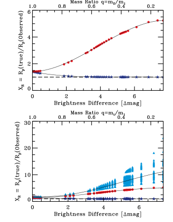
Figure 1.— Radii corrections factors ($X_{R}$) are plotted as a function of companion-to-primary brightness ratios (bottom axis) and mass ratios (top axis) for possible binary systems (top plot) or triple (bottom plot) systems. This figure is an example for the G-dwarf KOI-299; similar calculations have been made for every KOI. In each plot, the dark blue stars represent the correction factors if the planet orbits the primary star (equation 7); the red circles represent the correction factors if the planet orbits the secondary star, and the light blue triangles represent the correction factors if the planet orbits the tertiary star (equation 6). The lines are third order polynomials fit to the distributions. Unity is marked with a horizontal dashed line.

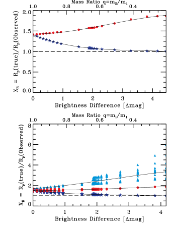
Figure 2.— This figure is the same as Figure 1, but for the M-dwarf KOI-1085, demonstrating that the details of the derived correction factors are dependent upon the KOI properties.

3. Possible Companions from Isochrones

To explore the possible effects of the undetected stellar companions on the derived planetary parameters, we first assess what companions are possible for each KOI. For this work, we have downloaded the Cumulative Kepler candidate list and stellar parameters table from the NASA Exoplanet Archive. The cumulative list is updated with each new release of the KOI lists; as a result, the details of any one star and planet may have changed since the analysis for this paper was done. However, the overall results of the paper presented here should remain largely unchanged.

For the KOI lists, the stellar parameters for each KOI were determined by fitting photometric colors and spectroscopically derived parameters (where available) to the Dartmouth Stellar Evolution Database (Dotter et al., 2008; Huber et al., 2014). The planet parameters were then derived based upon the transit curve fitting and the associated stellar parameters. Other stars listed in the Kepler Input Catalog or UKIRT imaging that may be blended with the KOI host stars were accounted for in the transit fitting, but, in general, as mentioned above, each planetary host star was assumed to be a single star.

We have restricted the range of possible bound stellar companions to each KOI host star by utilizing the same Dartmouth isochrones used to determine the stellar parameters. Possible gravitationally bound companions are assumed to lie along on the same isochrone as the primary star. For each KOI host star, we found the single best fit isochrone (characterized by mass, metallicity, and age) by minimizing the chi-square fit to the stellar parameters (effective temperature, surface gravity, radius, and metallicity) listed in the KOI table.

We did not try to re-derive stellar parameters or independently find the best isochrone fit for the star; we simply identified the appropriate Dartmouth isochrone as used in the determination of the stellar parameters (Huber et al., 2014). We note that there exists an additional uncertainty based upon the isochrone finding. In this work, we did not try to re-derive the stellar parameters of the host stars, but rather, we simply find the appropriate isochrone that matches the KOI stellar parameters. Thus, any errors in the stellar parameters derivations in the KOI list are propagated here. This is likely only a significant source of uncertainty for nearly equal brightness companions.

Once an isochrone was identified for a given star, all stars along an isochrone with (absolute) Kepler magnitudes fainter than the (absolute) Kepler magnitude of the host star were considered to be viable companions; i.e., the primary host star was assumed to be the brightest star in the system. The fainter companions listed within that particular isochrone were then used to establish the range of possible planetary radii corrections (equation 6) assuming the host star is actually a binary or triple star. Higher order (e.g., quadruple) stellar multiples are not considered here as they represent only $\sim 3$% of the stellar population (Raghavan et al., 2010).

Figure 3.— Top: The mean correction factor $\langle X_{R}\rangle$ for each KOI is displayed as a function of the effective temperature of the primary star (see section 4). The black curves are $3^{rd}$-order polynomials fitted to the distributions (equation 8). Bottom: Histograms of the correction factors displayed in the top panels. The vertical dashed lines mark the medians of the distributions. Left: The correction factors are computed for the Kepler Cumulative Kepler Objects of Interest list. Right: The corrections are computed for the KOIs but assuming the KOIs are 10 times closer as may be the case for K2 and TESS. The red points and histograms assume each KOI is single as is the case for the published KOI list; the blue points and histograms assume that each KOI has been vetted with radial velocity (RV) and high resolution imaging (HRI), and all stellar companions with orbital periods of 2 years or shorter and all stellar companions located at angular distances of $\geq 0.1^{\prime\prime}$ have been detected and accounted for in the planetary radii determinations (see Section 4.2). For the vetted stars, the correction factors are only for undetected stellar companions; detected companions have been assumed to be accounted for in the planet radii determinations.

We have considered six specific multiplicity scenarios:

1. single star ($X_{r}\equiv 1.0$)

2. binary star – planet orbits primary star

3. binary star – planet orbits secondary star

4. triple star – planet orbits primary star

5. triple star – planet orbits secondary star

6. triple star – planet orbits tertiary star.

Based upon the brightness and size differences between the primary star and the putative secondary or tertiary companions, we have calculated for each KOI the possible factor by which the planetary radii are underestimated ($X_{R}$). If the star is single, the correction factor is unity, and if, in a multiple star system, the planet orbits the primary star, only flux dilution affects the observed transit depth and the derived planetary radius (eq. 7).

For the scenarios where the planets orbits the secondary or tertiary star, the planet size correction factors (eq. 6) were determined only for stellar companions where the stellar companion could physically account for the observed transit depth. If more than 100% of the stellar companion light had to be eclipsed in order to produce the observed transit in the presence of the flux dilution, then that star (and all subsequent stars on the isochrone with lower mass) was not considered viable as a potential source of the transit. For example, for an observed 1% transit, no binary companions can be fainter than the primary star by 5 magnitudes or more; an eclipse of such a secondary star would need to be more than 100% deep. The stellar brightness limits were calculated independently for each planet within a KOI system so as to not assume that all planets within a system necessarily orbited the same star.

Figures 1 and 2 show representative correction factors ($X_{R}$) for KOI-299 (a G-dwarf with a super-Earth sized $R_{p}=1.8\pm 0.24R_{\oplus}$ planet) and for KOI-1085 (an M-dwarf with an Earth-sized $R_{p}=0.92\pm 0.13R_{\oplus}$ planet). The planet radius correction factors ($X_{R}$) are shown as a function of the companion–to–primary brightness ratio (bottom x-axis of plots) and the companion–to–primary mass ratio (top x-axis of plots) and are determined for the KOI assuming it is a binary-star system (top plot) or a triple-star system (bottom plot).

The amplitude of the correction factor ($X_{R}$) varies strongly depending on the particular system and which star the planet may orbit. If the planet orbits the primary star, then the largest the correction factors are for equal brightness companions ($\sqrt{2}\sim 1.4$ for a binary system and $\sqrt{3}\sim 1.7$ for a triple system) with an asymptotic approach to unity as the companion stars become fainter and fainter. If the planet orbits the secondary or tertiary star, the planet radius correction factor can be significantly larger – ranging from $X_{R}\gtrsim 2-5$ for binary systems and $X_{R}\gtrsim 2-20$ or more for triple systems – depending on the size and brightness of the secondary or tertiary star.

4. Mean Radii Correction Factors ($X_{R}$)

It is important to recognize the full range of the possible correction factors, but in order to have a better understanding of the statistical correction any given KOI (or the KOI list as a whole) may need, we must understand the mean correction for any one multiplicity scenario and convert these into a single mean correction factor for each star. To do this, we must take into account the probability the star may be a multiple star, the distribution of mass ratios if the star is a multiple, the probability that the planet orbits any one star if the stellar system has multiple stars, and whether or not the star has been vetted (and how well it is has been vetted) for stellar companions.

In order to calculate an average correction factor for each multiplicity scenario, we have fitted the individual scenario correction factors as a function of mass ratio with a 3^rd-order polynomial (see Fig. 1 and 2). Because the isochrones are not evenly sampled in mass, taking a mean straight from the isochrone points would skew the results; the polynomial parameterization of the correction factor as a function of the mass ratio enables a more robust determination of the mean correction factor for each multiplicity scenario.

If the companion–to–primary mass ratio distribution was uniform across all mass ratios, then a straight mean of the correction values determined from each polynomial curve would yield the average correction factor for each multiplicity scenario. However, the mass ratio distribution is likely not uniform, and we have adopted the form displayed in Figure 16 of Raghavan et al. (2010). That distribution is a nearly-flat frequency distribution across all mass ratios with a $\sim 2.5\times$ enhancement for nearly equal mass companion stars ($q\gtrsim 0.95$). This distribution is in contrast to the Gaussian distribution shown in Duquennoy & Mayor (1991); however, the more recent results of Raghavan et al. (2010) incorporate more stars, a broader breadth of stellar properties, and multiple companion detection techniques.

The mass ratio distribution is convolved with the polynomial curves fitted for each multiplicity scenario, and a weighted mean for each multiplicity scenario was calculated for every KOI. For example, in the case of KOI-299 (Fig. 1), the single star mean correction factor is 1.0 (by definition). For the binary star cases, the average scenario correction factors are 1.14 (planet orbits primary) and 2.28 (planet orbits secondary); for the triple stars cases, the correction factors are 1.16 (planet orbits primary), 2.75 (planet orbits secondary), and 4.61 (planet orbits tertiary). For KOI-1085 (Fig. 2), the weighted mean correction factors are 1.18, 1.56, 1.24, 1.61, and 2.29, respectively.

To turn these individual scenario correction factors into an overall single mean correction factor $\langle X_{R}\rangle$ per KOI, the six scenario corrections are convolved with the probability that a KOI will be a single star, a binary star, or a triple star. The multiplicity rate of the Kepler stars is still unclear (Wang et al., 2014b), and, indeed, there may be some contradictory evidence for the the exact value for the multiplicity rates of the KOI host stars (e.g., Horch et al., 2014; Wang et al., 2014b), but the multiplicity rates appear to be near $40\%$, similar to the general field population. In the absence of a more definitive estimate, we have chosen to utilize the multiplicity fractions from Raghavan et al. (2010): a 54% single star fraction, a 34% binary star fraction, and a 12% triple star fraction (Raghavan et al., 2010). We have grouped all higher order multiples ($3+$) into the single category of “triples”, given the relatively rarity of the quadruple and higher order stellar systems. For the scenarios where there are multiple stars in a system, we have assumed that the planets are equally likely to orbit any one of the stars (50% for binaries, 33.3% for triples).

The final mean correction factors $\langle X_{R}\rangle$ per KOI are displayed in Figure 3; the median value of the correction factor and the dispersion around that median is $\langle X_{R}\rangle=1.49\pm 0.12$. This median correction factor implies that assuming a star in the KOI list is single, in the absence of any (observational) companion vetting, yields a statistical bias on the derived planetary radii where the radii are underestimated, on average, by a factor $\sim 1.5$, and the mass density of the planets are overestimated by a factor of $\sim 1.5^{3}\sim 3$.

From Figure 3, it is clear that the mean correction factor $\langle X_{R}\rangle$ depends upon the stellar temperature of the host star. As most of the stars in the KOI list are dwarfs, the lower temperature stars are typically lower mass stars and, thus, have a smaller range of possible stellar companions. Thus, an average value for the correction factor 1.5 represents the sample as a whole, but a more accurate value for the correction factor can be derived for a given star, with a temperature between $3500\lesssim T_{eff}\lesssim 7500$K, using the fitted $3^{rd}$-order polynomial:

$$\langle X_{R}\rangle=a_{3}(T_{eff})^{3}+a_{2}(T_{eff})^{2}+a_{1}(T_{eff})+a_{0}$$ (8)

where $a_{3}=-1.19118\times 10^{-11},a_{2}=1.61749\times 10^{-7},a_{1}=-0.000560,{\ \rm and\ }a_{0}=1.64668$.

In the absence of any specific knowledge of the stellar properties (other than the effective temperature) and in the absence of any radial velocity or high resolution imaging to assess the specific companion properties of a given KOI, (see section 4.2), the above parameterization (equation 8) can be used to derive a mean radii correction factor $\langle X_{R}\rangle$ for a given star. For G-dwarfs and hotter stars, the correction factor is near $\langle X_{R}\rangle\sim 1.6$. As the stellar temperature (mass) of the primary decreases to the range of M-dwarfs, the correction factor can be as low as $\langle X_{R}\rangle\sim 1.2$.

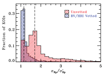
Figure 4.— The distribution of the ratio of the total planetary radii uncertainties ($\sigma_{R_{p}}$) to the quoted radii uncertainties ($\sigma^{\prime}_{R_{p}}$)from the cumulative KOI list (see equation 10). For the red histogram, it is assumed that the KOIs are single as is the case in the published KOI list; for the blue histogram, it is assumed that each KOI has been vetted with radial velocity (RV) and high resolution imaging (see Section 4.2). The vertical dashed lines represent the median values of the distributions: $\langle\sigma_{R_{p}}/\sigma^{\prime}_{R_{p}}\rangle=1.70$ for the unvetted KOIs and $\langle\sigma_{R_{p}}/\sigma^{\prime}_{R_{p}}\rangle=1.15$ for the vetted KOIs (see section 4.2).

4.1. Planet Radius Uncertainty Term from $\langle X_{R}\rangle$

The mean correction factor is useful for understanding how strongly the planetary radii may be underestimated, but an additional uncertainty term derived from the mean radius correction factor is potentially more useful as it can be added in quadrature to the formal planetary radii uncertainties. The formal uncertainties, presented in the KOI list, are derived from the uncertainties in the transit fitting and the uncertainty in the knowledge of the stellar radius, and they are calculated assuming the KOIs are single stars. We can estimate an additional planet radius uncertainty term based upon the mean radii correction factor as

$$\sigma_{X_{R}}=|\langle X_{R}\rangle R_{p}-R_{p}|=|\langle X_{R}\rangle-1.0|R_{p}$$ (9)

where $R_{p}$ is the observed radius of the planet. Adding in quadrature to the reported uncertainty, a more complete uncertainty on the planetary radius can be reported as

$$\sigma_{R_{p}}=\left((\sigma^{\prime}_{R_{p}})^{2}+(\sigma_{X_{R}})^{2}\right)^{1/2}$$ (10)

where $\sigma^{\prime}_{R_{p}}$ is the uncertainty of the planetary radius as presented in the KOI list.

The distribution of the ratio of the more complete KOI radius uncertainties ($\sigma_{R_{p}}$) to the reported KOI radius uncertainties ($\sigma^{\prime}_{R_{p}}$) is shown in Figure 4. Including the possibility that a KOI may be a multiple star increases the planetary radii uncertainties. While the distribution has a long tail dependent upon the specific system, the planetary radii uncertainties are underestimated as reported in the KOI list, on average, by a factor of 1.7.

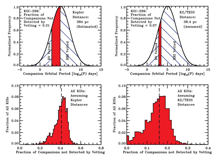
Figure 5.— Top Left: Example of the stellar companion period distribution that is vetted by radial velocity (RV) monitoring and high resolution imaging (HRI) for KOI-299. The Gaussian curve, normalized to unity, is the log-normal orbital period distribution of stellar companions (Raghavan et al., 2010), and the hatched regions mark where the potential observational vetting is assumed to have detected all companions in that period range. The solid (red) region of the Gaussian corresponds to the fraction of companions (31% for KOI-299) that would remain undetected by the RV and HRI observations (see section 4.2). Bottom Left: The distribution of the fraction of companions across all KOIs that remain undetected by observational radial velocity and high resolution imaging vetting (i.e., the red area in the top figure but for all KOIs). The vertical dashed line represents the median fraction ($41\%$) of companions left undetected by the observational vetting of all KOIs. Top Right: The same as the top left figure but assuming that KOI-299 is 10 times closer as may be the case for K2/TESS targets. At such a close distance for a hypothetical KOI-299, RV and HRI vetting leaves only about 7% of the possible stellar companions undetected. Bottom Right: As the bottom left figure but assuming all of the KOI host stars are 10 times closer as may be the case for K2/TESS. The vertical dashed line represents the median fraction ($16\%$) of companions left undetected if the KOIs were at these closer distances.

4.2. Effectiveness of Companion Vetting

The above analysis has assumed that the KOIs have undergone no companion vetting, as is the assumption in the current KOI list. In reality, the Kepler Project has funded a substantial ground-based follow-up observation program which includes radial velocity vetting and high resolution imaging. In this section, we explore the effectiveness of the observational vetting.

The observational vetting reduces the fraction of undetected companions. If there is no vetting or all stars are assumed to be single, as is the case for the published KOI list, then the fraction of undetected companions is 100% and the mean correction factors $\langle X_{R}\rangle$ are as presented above. If every stellar companion is detected and accounted for in the planetary parameter derivations, then the fraction of undetected companions is 0%, and the mean correction factors are unity. Reality is somewhere in between these two extremes.

To explore the effectiveness of the observational vetting on reducing the radii corrections factors (and the associated radii uncertainties), we have assumed that every KOI has been vetted equally, and all companions within the reach of the observations have been detected and accounted. Thus, the corrections factors depend only on the fraction of companions stars that remain out of the reach of vetting and undetected.

In this simulation, we have assumed that all companions with orbital periods of 2 years or less and all companions with angular separations of $0.1\arcsec$ or greater have been detected. This, of course, will not quite be true as random orbital phase effects, inclination effects, companion mass distribution, stellar rotation effects, etc. will diminish the efficiency of the observations to detect companions. We recognize the simplicity of these assumptions; however, the purpose of this section is to assess the usefulness of observational vetting on reducing the uncertainties of the planetary radii estimates, not to explore fully the sensitivities and completeness of the vetting.

Typical follow-up observations include stellar spectroscopy, a few radial velocity measurements, and high resolution imaging. The radial velocity observations usually include $2-3$ measurements over the span of $6-9$ months and are typically sufficient to identify potential stellar companions with orbital periods of $\lesssim 1-2$ years or less. While determining full orbits and stellar masses for any stellar companions detected typically requires more intensive observing, we have estimated that 3 measurements spanning $6-9$ months is sufficient to enable the detection of an RV trend for orbital periods of $\sim 2$ years or less and mark the star as needing more detailed observations. The amplitude of the RV signature, and hence the ability to detect companions, does depend upon the masses of the primary and companion stars; massive stars with low mass companions will display relatively low RV signatures. However, RV vetting for the Kepler program has been done at a level of $\lesssim 100-200$ m/s, which is sufficient to detect (at $\gtrsim 4-5\sigma$) a late-type M-dwarf companion in a two-year orbit around a mid B-dwarf primary. Indeed, the RV vetting is made even more effective by searching for companions via spectral signatures (Kolbl et al., 2015).

The high resolution imaging via adaptive optics, “lucky imaging”, and/or speckle observations typically has resolutions of $0.02\arcsec-0.1\arcsec$ (e.g., Howell et al., 2011; Horch et al., 2012; Lillo-Box et al., 2012; Adams et al., 2012, 2013; Dressing et al., 2014; Law et al., 2014; Lillo-Box et al., 2014; Wang et al., 2014a; Everett et al., 2014; Horch et al., 2014; Gilliland et al., 2014; Star et al., 2014). Based upon Monte Carlo simulations in which we have averaged over random orbital inclinations and eccentricities, we have calculated the fraction of time within its orbit a companion will be detectable via high resolution imaging. With typical high resolution imaging of 0.05″, we have estimated that $\gtrsim 50\%$ of the stellar companions will be detected at one full-width half-maximum (FWHM=0.05″) of the image resolution and beyond and $>90$% at $\gtrsim 2$ FWHM (0.1″) of the image resolution and beyond.

To determine what fraction of possible stellar companions would be detected in such a scenario, we have used the nearly log-normal orbital period distribution from Raghavan et al. (2010). To convert the high resolution imaging limits into period-limits, we have estimated the distance to each KOI by determining a distance modulus from the observed Kepler magnitude and the absolute Kepler magnitude associated with the fitted isochrone. The median distance to the KOIs was found to be $\sim 900$ pc, corresponding to $\sim 90$ AU for 0.1″ imaging. Using the isochrone stellar mass, the semi-major axis detection limits were converted to orbital period limits (assuming circular orbits).

Combining the 2-year radial velocity limit and the $0.1\arcsec$ imaging limit, we were able to estimate the fraction of undetected companions for each individual KOI (see Figure 5). The distribution of the fraction of undetected companions ranges from $\sim 20-60$% and, on average, the ground-based observations leave $\approx 41\%$ of the possible companions undetected for the KOIs (see Figure 5).

The mean correction factors $\langle X_{R}\rangle$ are only applicable to the undetected companions. For the stars that are vetted with radial velocity and/or high resolution imaging, the intrinsic stellar companion rate for the KOIs of 46% (Raghavan et al., 2010) is reduced by the unvetted companion fraction for each KOI. That is, we assume that companion stars detected in the vetting have been accounted for in the planetary radii determinations, and the unvetted companion fraction is the relevant companion rate for determining the correction factors. In the KOI-299 example (Fig. 5), the undetected companion rate used to calculate the mean radii correction factor is $0.46\times 0.31=0.1426$. This lower fraction of undetected companions in turn reduces the mean correction factors for the vetted stars which are displayed in Figure 3 (blue points).

Instead of a mean correction factor of $\langle X_{R}\rangle\sim 1.5$, the average correction factor is $\langle X_{R}\rangle=1.20\pm 0.06$ if the stars are vetted with radial velocity and high resolution imaging. The mean correction factor still changes as a function of the primary star effective temperature but the dependence is much more shallow with coefficients for equation 8 of $a_{3}=-6.73847\times 10^{-12},a_{2}=9.38966\times 10^{-8},a_{1}=-0.000352,{\ \rm and\ }a_{0}=1.40391$ (see Figure 3).

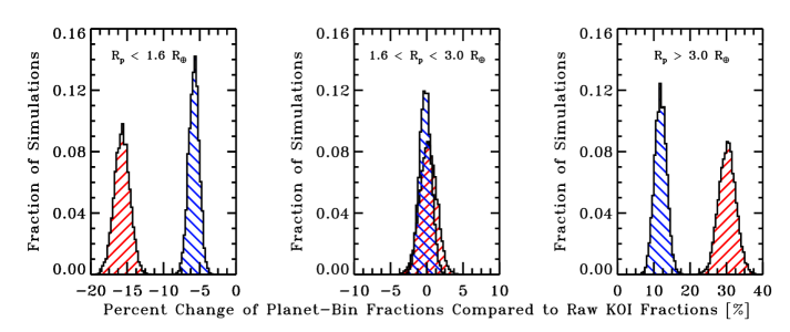
Figure 6.— The percent change of the measured occurrence rates from the raw KOI list (i.e., uncorrected for completeness) caused by undetected stellar companions and assuming all of the stars in the published KOI list are single. The fractional changes are computed for three different planet size bins as labeled in the plots. The results of assuming all the stars are single (i.e., unvetted) are in the red histogram and the results of vetting the all of the stars with radial velocity and high resolution imaging (section 4.2) are shown in the blue histogram. The histograms are based upon Monte Carlo simulations described in section 5

4.3. K2 and TESS

The above analysis has concentrated on the Kepler Mission and the associated KOI list, but the same effects will apply to all transit surveys including K2 (Howell et al., 2014) and TESS (Ricker et al., 2014). If the planetary host stars from K2 and TESS are also assumed to be single with no observational vetting, the planetary radii will be underestimated by the same amount as the Kepler KOIs (Fig. 3 and eq. 8).

Many K2 targets and nearly all of TESS targets will be stars that are typically $4-5$ magnitudes brighter than the stars observed by Kepler, and therefore, K2 and TESS targets will be $\sim 10$ times closer than the Kepler targets. The effectiveness of the radial velocity vetting will remain mostly unaffected by the brighter and closer stars, but the effectiveness of the high resolution imaging will be significantly enhanced. Instead of probing the stars to within $\sim 100$AU, the imaging will be able to detect companion stars within $\sim 10$ AU of the stars.

As a result, the fraction of undetected companions will decrease significantly. Even for the Kepler stars that undergo vetting via radial velocity and high resolution imaging, $\sim 40$% of the companions remain undetected. But for the stars that are 10 times closer that fraction decreases to $\sim 16$% (see Figure 5). This has the strong benefit of greatly reducing the mean correction factors for the stars that are observed by K2 and TESS and are vetted for companions with radial velocity and high resolution imaging.

The mean correction factor for vetted K2/TESS-like stars is only $\langle X_{R}\rangle=1.07\pm 0.03$. The correction factor has a much flatter dependence on the primary star effective temperature, because the majority of the possible stellar companions are detected by the vetting. The coefficients for equation 8 become $a_{3}=-4.12309\times 10^{-12},a_{2}=5.89709\times 10^{-8},a_{1}=-0.000242,{\ \rm and\ }a_{0}=1.30060$. The mean radii correction factors for vetted K2/TESS planetary host stars correspond to a correction to the planetary radii uncertainties of only $\sim 2$%, in comparison to a correction of $\sim 70$% if the K2/TESS stars remain unvetted.

For K2 and TESS, where the number of candidate planetary systems may outnumber the KOIs by an order of magnitude (or more), single epoch high resolution imaging may prove to be the most important observational vetting performed. While the imaging will not reach the innermost stellar companions, radial velocity observations require multiple visits over a baseline comparable to the orbital periods an observer is trying to sample. In contrast, the high resolution imaging requires a single visit (or perhaps one per filter on a single night) and will sample the majority of the expected stellar companion period distribution.

5. Effect of Undetected Companions on the Derived Occurrence Rates

Understanding the occurrence rates of the Earth-sized planets is one of the primary goals of the Kepler mission and one of the uses of the KOI list (Borucki et al., 2010). It has been shown that the transition from ”rocky” to ”non-rocky” planets occurs near a radius of $R_{p}=1.6\ R_{\oplus}$ and the transition is very sharp (Rogers, 2014). However, the amplitude of the uncertainties resulting from undetected companions may be large enough to push planets across this boundary and affect our knowledge of the fraction of Earth-sized planets.

We have explored the possible effects of undetected companions on the derived occurrence rates. The planetary radii can not simply be multiplied by a mean correction factor $X_{R}$, as that factor is only a measure of the statistical uncertainty of the planetary radius resulting from assuming the stars are single and only a fraction of the stars are truly multiples. Instead a Monte Carlo simulation has been performed to assign randomly the effect of unseen companions on the KOIs.

The simulation was performed 10,000 times for each KOI. For each realization of the simulation, we have randomly assigned the star to be single, binary, or triple star via the 54%, the 34% and the 12% fractions (Raghavan et al., 2010). If the KOI is assigned to be a single star, the mean correction factors for the planets in that system are unity: $\langle X_{R}\rangle=1$. If the KOI star is a multiple star system, we have randomly assigned the stellar companion masses according to the masses available from the fitted isochrones and using the mass ratio distribution of (Raghavan et al., 2010). Finally, the planets are randomly assigned to the primary or to the companion stars (i.e., 50% fractions for binary stars and 33.3% fractions for triple stars). Once the details for the system are set for a particular realization, the final correction factor for the planets are determined from the polynomial fits for the individual multiplicity scenarios (e.g., Fig. 1 and 2).

For each set of the simulations, we compiled the fraction of planets within the following planet-radii bins: $R_{p}\leq 1.6\ R_{\oplus}$; $1.6<R_{p}\leq 3.0\ R_{p}$; $3.0<R_{p}\leq 10\ R_{\oplus}$ corresponding to Earth-sized, super-Earth/mini-Neptune-sized, and Neptune-to-Jupiter-sized planets. The raw fractions directly from the KOI-list, for these three categories of planets, are 33.3%, 46.0%, and 20.7%. Note that these are the raw fractions and are not corrected for completeness or detectability as must be done for a true occurrence rate calculation; these fractions are necessary for comparing how unseen companions affect the determination of fractions. Finally, we repeated the simulations, but using the undetected multiple star fractions after vetting with radial velocity and high resolution imaging had been performed, thus, effectively increasing the fraction of stars with correction factors of unity.

The distributions of the change in the fractions of planets in each planet category, compared to the raw KOI fractions, are shown in Figure 6. If the occurrence rates utilize the assumed-single KOI list (i.e., unvetted), then the Earth-sized planet fraction may be overestimated by as much as $15-20$% and the giant-planet fraction may be underestimated by as much as 30%. Interestingly, the fraction of super-Earth/mini-Neptune planets does not change substantially; this is a result of smaller planets moving into this bin, and larger planets moving out of the bin. In contrast, if all of the KOIs undergo vetting via radial velocity and high resolution imaging, the fractional changes to these bin fractions are much smaller: $5-7$% for the Earth-sized planets and $10-12$% for the Neptune/Jupiter-sizes planets.

6. Summary

We present an exploration of the effect of undetected companions on the measured radii of planets in the Kepler sample. We find that if stars are assumed to be single (as they are in the current Kepler Objects of Interest list) and no companion vetting with radial velocity and/or high resolution imaging is performed, the planetary radii are underestimated, on average, by a factor of $\langle X_{R}\rangle=1.5$, corresponding to an overestimation of the planet bulk density by a factor of $\sim 3$. Because lower mass stars will have a smaller range of stellar companion masses than higher mass stars, the planet radius mean correction factor has been quantified as a function of stellar effective temperature.

If the KOIs are vetted with radial velocity observations and high resolution imaging, the planetary radius mean correction necessary to account for undetected companions is reduced significantly to a factor of $\langle X_{R}\rangle=1.2$. The benefit of radial velocity and imaging vetting is even more powerful for missions like K2 and TESS, where the targets are, on average, ten times closer than the Kepler Objects of Interest. With vetting, the planetary radii for K2 and TESS targets will only be underestimated, on average, by 10%. Given the large number of candidates expected to be produced by K2 and TESS, single epoch high resolution imaging may be the most effective and efficient means of reducing the mean planetary radius correction factor.

Finally, we explored the effects of undetected companions on the occurrence rate calculations for Earth-sized, super-Earth/mini-Neptune-sized, and Neptune-sized and larger planets. We find that if the Kepler Objects of Interest are all assumed to be single (as they currently are in the KOI list), then the fraction of Earth-sized planets may be overestimated by as much as 15-20% and the fraction of large planets may be underestimated by as much as 30%

The particular radial velocity observations or high resolution imaging vetting that any one KOI may (or may not) have undergone differs from star to star. Companion vetting simulations presented here show that a full understanding and characterization of the planetary companions is dependent upon also understanding the presence of stellar companions, but is also dependent upon understanding the limits of those observations. For a final occurrence rate determination of Earth-sized planets and, more importantly, an uncertainty on that occurrence rate, the stellar companion detections (or lack thereof) must be taken into account.

References

- Adams et al. (2012) Adams, E. R., Ciardi, D. R., Dupree, A. K., et al. 2012, AJ, 144, 42
- Adams et al. (2013) Adams, E. R., Dupree, A. K., Kulesa, C., & McCarthy, D. 2013, AJ, 146, 9
- Batalha et al. (2011) Batalha, N. M. et al. 2011, ApJ, 729, 27
- Batalha (2014) Batalha, N. M. 2014, Proceedings of the National Academy of Science, 111, 12647
- Borucki et al. (2010) Borucki, W. J., et al. 2010, Science, 327, 977
- Brown et al. (2011) Brown, T. M., Latham, D. W., Everett, M. E., & Esquerdo, G. A. 2011, AJ, 142, 112
- Burke et al. (2014) Burke, C. J., Bryson, S. T., Mullally, F., et al. 2014, ApJS, 210, 19
- Ciardi et al. (2013) Ciardi, D. R., Fabrycky, D. C., Ford, E. B., et al. 2013, ApJ, 763, 41
- Dotter et al. (2008) Dotter, A., Chaboyer, B., Jevremović, D., et al. 2008, ApJS, 178, 89
- Dressing & Charbonneau (2013) Dressing, C. D., & Charbonneau, D. 2013, ApJ, 767, 95
- Dressing et al. (2014) Dressing, C. D., Adams, E. R., Dupree, A. K., Kulesa, C., & McCarthy, D. 2014, AJ, 148, 78
- Duquennoy & Mayor (1991) Duquennoy, A., & Mayor, M. 1991, A&A, 248, 485
- Everett et al. (2014) Everett, M. E., Barclay, T., Ciardi, D. R., et al. 2014, arXiv:1411.3621
- Fressin et al. (2013) Fressin, F., Torres, G., Charbonneau, D., et al. 2013, ApJ, 766, 81
- Gilliland et al. (2014) Gilliland, R. L., Cartier, K. M. S., Adams, E. R., et al. 2014, arXiv:1407.1009
- Horch et al. (2012) Horch, E. P., Howell, S. B., Everett, M. E., & Ciardi, D. R. 2012, AJ, 144, 165
- Horch et al. (2014) Horch, E. P., Howell, S. B., Everett, M. E., & Ciardi, D. R. 2014, ApJ, 795, 60
- Howell et al. (2011) Howell, S. B., Everett, M. E., Sherry, W., Horch, E., & Ciardi, D. R. 2011, AJ, 142, 19
- Howell et al. (2014) Howell, S. B., et al., 2014, PASP, 126, 398
- Huber et al. (2014) Huber, D., Silva Aguirre, V., Matthews, J. M., et al. 2014, ApJS, 211, 2
- Howard et al. (2012) Howard, A. W., Marcy, G. W., Bryson, S. T., et al. 2012, ApJS, 201, 15
- Kolbl et al. (2015) Kolbl, R., Marcy, G. W., Isaacson, H., & Howard, A. W. 2015, AJ, 149, 18
- Law et al. (2014) Law, N. M., Morton, T., Baranec, C., et al. 2014, ApJ, 791, 35
- Lillo-Box et al. (2012) Lillo-Box, J., Barrado, D., & Bouy, H. 2012, A&A, 546, AA10
- Lillo-Box et al. (2014) Lillo-Box, J., Barrado, D., & Bouy, H. 2014, A&A, 566, AA103
- Marcy et al. (2014) Marcy, G. W., Isaacson, H., Howard, A. W., et al. 2014, ApJS, 210, 20
- Morton & Johnson (2011) Morton, T. D., & Johnson, J. A. 2011, ApJ, 738, 170
- Morton (2012) Morton, T. D. 2012, ApJ, 761, 6
- Mullally et al. (2014) Mullally, F. et al. 2015, ApJ, submitted
- Petigura et al. (2013) Petigura, E. A., Howard, A. W., & Marcy, G. W. 2013, Proceedings of the National Academy of Science, 110, 19273
- Raghavan et al. (2010) Raghavan, D., McAlister, H. A., Henry, T. J., et al. 2010, ApJS, 190, 1
- Ricker et al. (2014) Ricker, G. R., Winn, J. N., Vanderspek, R., et al. 2014, Proc. SPIE, 9143, 914320
- Rogers (2014) Rogers, L. A. 2014, arXiv:1407.4457
- Star et al. (2014) Star, K. M., Gilliland, R. L., Wright, J. T., & Ciardi, D. R. 2014, arXiv:1407.1057
- Wang et al. (2014a) Wang, J., Xie, J.-W., Barclay, T., & Fischer, D. A. 2014, ApJ, 783, 4
- Wang et al. (2014b) Wang, J., Fischer, D. A., Xie, J.-W., & Ciardi, D. R. 2014, ApJ, 791, 111
- Wang et al. (2014c) Wang, J., Fischer, D. A., Horch, E. P., & Huang, X. 2014, arXiv:1412.1731