Connecting Angular Momentum and Galactic Dynamics: The Complex Interplay between Spin, Mass, and Morphology

Abstract

The evolution and distribution of the angular momentum of dark matter (DM) halos have been discussed in several studies over the past decades. In particular, the idea arose that angular momentum conservation should allow to infer the total angular momentum of the entire DM halo from measuring the angular momentum of the baryonic component, which is populating the center of the halo, especially for disk galaxies. To test this idea and to understand the connection between the angular momentum of the DM halo and its galaxy, we use a state-of-the-art, hydrodynamical cosmological simulation taken from the set of Magneticum Pathfinder simulations. Thanks to the inclusion of the relevant physical processes, the improved underlying numerical methods, and high spatial resolution, we successfully produce populations of spheroidal and disk galaxies self-consistently. Thus, we are able to study the dependence of galactic properties on their morphology. We find that (1) the specific angular momentum of stars in disk and spheroidal galaxies as a function of their stellar mass compares well with observational results; (2) the specific angular momentum of the stars in disk galaxies is slightly smaller compared to the specific angular momentum of the cold gas, in good agreement with observations; (3) simulations including the baryonic component show a dichotomy in the specific stellar angular momentum distribution when splitting the galaxies according to their morphological type (this dichotomy can also be seen in the spin parameter, where disk galaxies populate halos with slightly larger spin compared to spheroidal galaxies); (4) disk galaxies preferentially populate halos in which the angular momentum vector of the DM component in the central part shows a better alignment to the angular momentum vector of the entire halo; and (5) the specific angular momentum of the cold gas in disk galaxies is approximately 40% smaller than the specific angular momentum of the total DM halo and shows a significant scatter.

1. Introduction

The question of how the different types of galaxies formed, and, in particular, which properties determine a galaxy to become a disk or spheroidal, has been a matter of debate since the discovery that the Universe is full of distant stellar islands of different morphology. For elliptical galaxies the following formation scenarios are discussed: from observations of ongoing mergers between galaxies of similar masses we know that spheroids can form in a major merger event between (spiral) galaxies. This has been supported by many simulations (e.g., Toomre 1977; White 1978, 1979; Barnes & Hernquist 1996; Naab et al. 2006). However, this scenario is not sufficient to explain certain observational properties, especially for the most massive galaxies. Thus, an alternative formation scenario through a series of multiple minor merger events was proposed by Meza et al. (2003) and established by, e.g., Naab et al. (2009), González-García et al. (2009), Oser et al. (2010), and Johansson et al. (2012).

For the formation scenarios of spiral galaxies, the details of their formation processes are less well known, but all the different channels discussed in the literature over the past decades are connected to the detailed buildup of the angular momentum and how the gaseous component transports intrinsic angular momentum into the central part of the halo, where the galaxy assembles. Initially, the dark matter (DM) halo and the infalling gas have identical angular momenta, but during the formation of the galaxy the gas cools and condenses in the center of the halo to form a disk. Assuming that the angular momentum of the gas is conserved during this process, the angular momentum of the halo of a disk galaxy can be estimated directly from the angular momentum of the disk of the galaxy (Fall & Efstathiou, 1980; Fall, 1983; Mo et al., 1998).

In hierarchical scenarios of structure formation, structures form through the gathering of clumps owing to the gravitational force (Peebles, 1993, and references therein). The DM collapses at high redshifts into small objects, which grow into larger objects through merging and finally build halos. Those halos are not completely spherically symmetric owing to tidal torques induced by neighboring halos. The baryons condense in the centers of these DM halos and form the first protogalaxies (White & Rees, 1978). Since the baryons and the DM originally gained the same amount of angular momentum through these tidal torques (Peebles, 1969; Doroshkevich, 1970) and the angular momentum of the gas should be conserved during the collapse, the disk is expected to have a similar specific angular momentum to that of its hosting halo (Fall & Efstathiou, 1980).

In contrast to observations, numerical $N$-body simulations have the advantage that structures can be followed through time, enabling the detailed understanding of the early stages of galaxy formation. Until recently, simulations using traditional smoothed particle hydrodynamics (SPH) codes suffered from the so-called angular momentum problem, where the objects became too small compared to observations because the gas had lost too much angular momentum (e.g., Navarro & Benz, 1991; Navarro & White, 1994; Navarro & Steinmetz, 1997). Sijacki et al. (2012) showed that SPH simulations overestimate the number of elliptical galaxies owing to the lower amount of mixing, and therefore causing this spurious “angular momentum crisis” of the baryons. On the opposite side, adaptive mesh refinement (AMR) or moving mesh simulations tend to overpredict the amount of disk-like galaxies in the absence of any feedback (Scannapieco et al., 2012). As simulations become better in resolution and also include feedback from stars, supernovae (SNe), and active galactic nuclei (AGNs), the gas is prevented from cooling too soon. Hence, early star formation is suppressed and the associated loss of angular momentum can be minimized. There are several studies that investigate the influence of star formation and the associated SN feedback on the formation of galactic disks (e.g., Brook et al., 2004; Okamoto et al., 2005; Governato et al., 2007; Scannapieco et al., 2008; Zavala et al., 2008). They find that strong feedback at early times leads to the formation of more realistic disk galaxies. A more recent study on the effect of stellar feedback on the angular momentum is presented in Übler et al. (2014), where they found that strong feedback favors disk formation. A recent, detailed summary of disk galaxy simulations can be found in Murante et al. (2015).

One parameter to describe the rotation of a system is the so-called spin parameter $\lambda$, which was introduced by Peebles (1969, 1971) and has since been investigated in several studies. With $\lambda$ it is possible to measure the degree of rotational support of the total halo. It has the advantage that it is only weakly depending on the halo’s mass and its internal substructures (Barnes & Efstathiou, 1987). The connection of this parameter with galaxy formation has been studied by many authors.

At first, DM-only simulations were employed. Bullock et al. (2001) introduced a modified version of the $\lambda$-parameter by defining the energy of the halo via its circular velocity. In addition, they studied the alignment of the angular momentum of the inner and outer halo parts. They found that most halos were well aligned but that about 10% of the halos showed a misalignment. Aubert et al. (2004) investigated the alignment between the inner spin of halos and the angular momentum of the outer halo and also the alignment between the inner spin and the angular momentum of the inflowing material. The misalignment angle of the angular momentum vectors at different radii was studied in more detail by Bailin & Steinmetz (2005), who showed that with increasing separation of the radii the misalignment of the vectors increases. In another study, Macciò et al. (2008) focused on the spin parameter’s dependency on the mass and the cosmology and found no correlations. Trowland et al. (2013) studied the connection of the halo spin with the large-scale structure. They confirmed that the spin parameter is not mass dependent at low redshift but found a tendency to smaller spins at higher redshifts.

Other authors included nonradiative gas in their analysis. The misalignment of the gas and DM angular momentum vectors and their spin parameters at redshift $z=3$ were investigated by van den Bosch et al. (2002). They found the angular momentum vectors to be misaligned by a median angle of about $30^{\circ}$. However, the overall distributions of the spin parameters of the gas and the DM were found to be very similar. Another detailed study by Sharma & Steinmetz (2005) and Sharma et al. (2012) found that the spin parameter of the gas component is on average higher than that of the DM, and they reported a misalignment of the angular momentum of the gas and the DM of about $20^{\circ}$.

Chen et al. (2003) compared the spin parameter and the misalignment angles between the DM and gas angular momentum vectors obtained in simulations, which include radiative cooling. This enables a splitting of the gas into a cold and a hot component. In their nonradiative model they confirmed that the spin parameter of the gas component has higher spin than the DM, while in their simulations with cooling the two components had approximately the same spin. The misalignments of the global angular momentum vectors were $22.8^{\circ}$ and $25^{\circ}$ for the two different cooling models and $23.5^{\circ}$ for the nonradiative case. Stewart et al. (2011, 2013) focused on the specific angular momentum and the spin parameter in relation to the cold/hot mode accretion by following the evolution of individual halos over cosmic time. They found that the spin of cold gas was the highest compared to all other components and about $3-5$ times higher than that of the DM component. Scannapieco et al. (2009) investigated the evolution of eight individual halos from zoom simulations and did not find a correlation between the spin parameter and the morphology of the galaxy. However, they found a correlation between the morphology and the specific angular momentum: for disks, the specific angular momentum can be higher than that of the host halo, while spheroids tend to have lower specific angular momentum. In addition, they saw a misalignment between stellar disks and infalling cold gas. Also, Sales et al. (2012) reported no correlation between the spin parameter and the galaxy type and concluded that disks are predominantly formed in halos where the freshly accreted gas has similar angular momentum to that of earlier accretion, whereas spheroids tend to form in halos where gas streams in along misaligned cold flows. The angular momentum properties of the inflowing gas were studied by Pichon et al. (2011). They found that the angular momentum of the cold dense gas is well aligned with the angular momentum of the DM halo, in contrast to the hot diffuse gas. Additionally, an increase of the advected specific angular momentum of the gas component with cosmic time was noticed. They proposed a scenario in which the angular momentum of the galaxies is fed by the collimated cold flows that are amplified with time and make the disks larger. Kimm et al. (2011) studied the different behavior of the gas and DM specific angular momentum by following the evolution of a Milky-Way-type galaxy over cosmic time. They also found that the gas has higher specific angular momentum and spin parameter than the DM. Hahn et al. (2010) investigated a sample of about 100 galactic disks and their alignment with their host halo at three different redshifts. Both the stellar and gas disks had a median misalignment angle of about $49^{\circ}$ with respect to the hosting DM halo at $z=0$.

Some works focused explicitly on the effect that baryons have on the DM halo by running parallel DM-only simulations. Bryan et al. (2013), who extracted halos from OWLS (Schaye et al., 2010), did not find a dependency of the spin parameter on mass, redshift, or cosmology in their DM-only runs. In the simulations that included baryons and strong feedback, the overall spin was found to be affected only very little, while the baryons had a noticeable influence on the inner halo, independent of the feedback strength. Bett et al. (2010) investigated the specific angular momentum and the misalignment of the galaxy with its halo. They obtained a median misalignment angle of about $25^{\circ}$ for the DM-only runs and about $30^{\circ}$ for the run including baryons. The baryons were found to spin up the inner region of the halo.

Recently, Welker et al. (2014) studied the alignment of the galaxy spins with their surrounding filaments, using the Horizon-AGN simulation (Dubois et al., 2014). They find that halos experiencing major mergers often lower the spin, while in general minor mergers can increase the amount of angular momentum. If a halo does not undergo any mergers but only smooth accretion, the spin of the galaxy increases with time, in contrast to that of its hosting DM halo. Since the gas streams and clumps in general move along the filaments, the galaxies realign with their filaments. Danovich et al. (2015) have investigated the buildup of the angular momentum in galaxies, using a sample of 29 resimulated galaxies at redshifts from $z=4$ to $1.5$. Overall the spin of the cold gas was about three times higher than that of the DM halo, in line with previous studies. Genel et al. (2015) explored the importance of stellar and AGN feedback for the evolution of the angular momentum of the galaxies in the Illustris simulations, finding the angular momentum of their simulated galaxies to be in good agreement with observations for a chosen feedback similar to the one used in this paper.

Observations indicate that the morphology of galaxies is strongly influenced by the relation between mass and angular momentum (see Fall, 1983). The angular momentum of disk galaxies was found to be about six times higher than that of the ellipticals of equal mass. Romanowsky & Fall (2012) and Fall & Romanowsky (2013) revisited and extended this work, analyzing 67 spiral and 40 early-type galaxies. They found that lenticular (S0) galaxies lie between spiral and elliptical galaxies in the so-called $M_{\mathrm{star}}-j_{\mathrm{star}}$-plane. The bulges of spiral galaxies follow a similar relation because they behave like “mini-ellipticals.” Obreschkow & Glazebrook (2014) used data from high-precision measurements of 16 nearby spiral galaxies to calculate the specific angular momentum of the gas and the stars. They confirmed observationally that the mass and angular momentum are strongly correlated with the morphology of galaxies. Hernandez & Cervantes-Sodi (2006) calculated the $\lambda$-parameter for two galaxy samples with a total of 337 observed spirals and found that with decreasing bulge-to-disk ratio the spirals have increasing $\lambda$-values. In a further study Hernandez et al. (2007) investigated a sample of 11,597 spiral and elliptical galaxies from the Sloan Digital Sky Survey (SDSS) and found that ellipticals on average have lower $\lambda$-values than spiral galaxies.

Recently, a new generation of cosmological, hydrodynamical simulations, e.g., the MassiveBlack-II (Khandai et al., 2015), Magneticum Pathfinder (Hirschmann et al., 2014), Illustris (Vogelsberger et al., 2014), Horizon-AGN (Dubois et al., 2014), and EAGLE (Schaye et al., 2015) simulations, have been employed to follow the evolution of structures in the Universe. A new aspect of such simulations is that for the first time reasonable galaxy morphologies can be associated with the galaxies formed in those simulations, e.g., Horizon-AGN (Dubois et al., 2014), Illustris (Torrey et al., 2015), EAGLE (Schaye et al., 2015), and Magneticum Pathfinder (Remus et al., 2015). In this work we will analyze simulations from the set of Magneticum Pathfinder simulations (K. Dolag et al., in preparation), which are introduced in Section 2, and investigate how the baryonic component influences the morphology of the galaxy. In Section 3 we introduce the formulae and investigate the angular momentum, the spin parameter, and the alignments of halos. In Section 4 we show the kinematical split-up of galaxies, which allows us to classify the galaxies in the simulation using the circularity parameter $\varepsilon$ in Section 5. We then examine the angular momentum of the different components of spheroids and disks. Furthermore, we study the alignment of the angular momentum vectors of the baryonic and the DM component. Additionally, we analyze the differences in the spin parameter $\lambda$ of spheroidal and disk galaxies.

2. The Magneticum Pathfinder Simulations

In order to study the properties of galaxies in a statistically relevant manner, we need both a large sample size and high enough resolution to resolve the morphology and underlying physics of galaxies. Since the newest generation of cosmological simulations can achieve both, they are a valuable tool for this study. We take the galaxies for our studies from the Magneticum Pathfinder simulations, which are a set of cosmological hydrodynamical simulations with different volumes and resolutions (K. Dolag et al., in preparation). The simulations were performed with an extended version of the $N$-body/SPH code GADGET-3, which is an updated version of GADGET-2 (Springel et al., 2001b; Springel, 2005). It includes various updates in the formulation of SPH regarding the treatment of the viscosity and the used kernels (see Dolag et al., 2005; Donnert et al., 2013; Beck et al., 2015).

It also allows a treatment of radiative cooling, heating from a uniform time-dependent ultraviolet (UV) background, and star formation with the associated feedback processes. The latter is based on a subresolution model for the multiphase structure of the interstellar medium (Springel & Hernquist, 2003). Radiative cooling rates are computed following the same procedure presented by Wiersma et al. (2009). We account for the presence of the cosmic microwave background (CMB) and of UV/X-ray background radiation from quasars and galaxies, as computed by Haardt & Madau (2001). The contributions to cooling from each one of 11 elements (H, He, C, N, O, Ne, Mg, Si, S, Ca, Fe) have been precomputed using the publicly available CLOUDY photoionization code (Ferland et al., 1998) for an optically thin gas in (photo)ionization equilibrium.

In the multiphase model for star formation (Springel & Hernquist, 2003), the ISM is treated as a two-phase medium where clouds of cold gas form from cooling of hot gas and are embedded in the hot gas phase assuming pressure equilibrium whenever gas particles are above a given threshold density. The hot gas within the multiphase model is heated by SNe and can evaporate the cold clouds. A certain fraction of massive stars (10%) is assumed to explode as SNe II. The released energy by SNe II ($10^{51}$ erg) is modeled to trigger galactic winds with a mass loading rate being proportional to the star formation rate (SFR) to obtain a resulting wind velocity of $v_{\mathrm{wind}}=350$km/s. Our simulations also include a detailed model of chemical evolution according to Tornatore et al. (2007). Metals are produced by SNe II, by SNe Ia, and by intermediate- and low-mass stars in the asymptotic giant branch (AGB). Metals and energy are released by stars of different mass by properly accounting for mass-dependent lifetimes (with a lifetime function according to Padovani & Matteucci, 1993), the metallicity-dependent stellar yields by Woosley & Weaver (1995) for SNe II, the yields by van den Hoek & Groenewegen (1997) for AGB stars, and the yields by Thielemann et al. (2003) for SNe Ia. Stars of different mass are initially distributed according to a Chabrier initial mass function (Chabrier, 2003).

Most importantly, our simulations also include a prescription for black hole (BH) growth and for feedback from AGNs based on the model presented in Springel et al. (2005) and Di Matteo et al. (2005), including the same modifications as in the study of Fabjan et al. (2010) and some new, minor changes.

As for star formation, the accretion onto BHs and the associated feedback adopt a subresolution model. BHs are represented by collisionless “sink particles” that can grow in mass by accreting gas from their environments, or by merging with other BHs. The gas accretion rate $\dot{M}_{\bullet}$ is estimated using the Bondi-Hoyle-Lyttleton approximation (Hoyle & Lyttleton, 1939; Bondi & Hoyle, 1944; Bondi, 1952):

$$\dot{M}_{\bullet}=\frac{4\pi G^{2}M_{\bullet}^{2}f_{\mathrm{b}oost}\rho}{(c_{s}^{2}+v^{2})^{3/2}},$$ (1)

where $\rho$ and $c_{s}$ are the density and the sound speed of the surrounding (ISM) gas, respectively, $f_{\mathrm{b}oost}$ is a boost factor for the density, which typically is set to $100$ and $v$ is the velocity of the BH relative to the surrounding gas. The BH accretion is always limited to the Eddington rate (maximum possible accretion for balance between inward-directed gravitational force and outward-directed radiation pressure): $\dot{M}_{\bullet}=\min(\dot{M}_{\bullet},\dot{M}_{\mathrm{edd}})$. Note that the detailed accretion flows onto the BHs are unresolved, and thus we can only capture BH growth due to the larger-scale gas distribution, which is resolved. Once the accretion rate is computed for each BH particle, the mass continuously grows. To model the loss of this gas from the gas particles, a stochastic criterion is used to select the surrounding gas particles to be removed. Unlike in Springel et al. (2005), in which a selected gas particle contributes with all its mass, we included the possibility for a gas particle to lose only a slice of its mass, which corresponds to 1/4 of its original mass. In this way, each gas particle can contribute with up to four ‘generations’ of BH accretion events, thus providing a more continuous description of the accretion process.

The radiated luminosity $L_{\mathrm{r}}$ is related to the BH accretion rate by $L_{\mathrm{r}}=\epsilon_{\mathrm{r}}\dot{M}_{\bullet}c^{2}$, where $\epsilon_{\mathrm{r}}$ is the radiative efficiency, for which we adopt a fixed value of 0.1 (standardly assumed for a radiatively efficient accretion disk onto a nonrapidly spinning BH according to Shakura & Sunyaev, 1973, see also Springel, 2005; Di Matteo et al., 2005). We assume that a fraction $\epsilon_{\mathrm{f}}$ of the radiated energy is thermally coupled to the surrounding gas so that $\dot{E}_{\mathrm{f}}=\epsilon_{\mathrm{r}}\epsilon_{\mathrm{f}}\dot{M}_{\bullet}c^{2}$ is the rate of the energy feedback; $\epsilon_{\mathrm{f}}$ is a free parameter and typically set to $0.1$ (see discussion in Steinborn et al. (2015)). The energy is distributed kernel weighted to the surrounding gas particles in an SPH-like manner. Additionally, we incorporated the feedback prescription according to Fabjan et al. (2010): we account for a transition from a quasar- to a radio-mode feedback (see also Sijacki et al., 2007) whenever the accretion rate falls below an Eddington ratio of $f_{\mathrm{edd}}:=\dot{M}_{\mathrm{r}}/\dot{M}_{\mathrm{edd}}<10^{-2}$. During the radio-mode feedback we assume a 4 times larger feedback efficiency than in the quasar mode. This way, we want to account for massive BHs, which are radiatively inefficient (having low accretion rates), but which are efficient in heating the ICM by inflating hot bubbles in correspondence to the termination of AGN jets. Note that we also, in contrast to Springel et al. (2005), modify the mass growth of the BH by taking into account the feedback, e.g., $\Delta M_{\bullet}=(1-\eta_{r})\dot{M}_{\bullet}\Delta t$. Additionally, we introduced some technical modifications of the original implementation, for which readers can find details in Hirschmann et al. (2014), where we also demonstrate that the bulk properties of the AGN population within the simulation are similar to observed AGN properties.

The simulation additionally follows thermal conduction, similar to Dolag et al. (2004), but with a choice of 1/20 of the classical Spitzer value (Spitzer, 1962). The choice of a suppression value significantly below 1/3 can be justified by comparison with full MHD simulations including an anisotropic treatment of thermal conduction (see discussion in Arth et al. (2014)).

The initial conditions are using a standard $\Lambda$CDM cosmology with parameters according to the seven-year results of the Wilkinson Microwave Anisotropy Probe (WMAP7; Komatsu et al. 2011). The Hubble parameter is $h=0.704$, and the density parameters for matter, dark energy, and baryons are $\Omega_{M}=0.272$, $\Omega_{\Lambda}=0.728$, and $\Omega_{b}=0.0451$, respectively. We use a normalization of the fluctuation amplitude at 8 Mpc of $\sigma_{8}=0.809$ and also include the effects of baryonic acoustic oscillations.

The Magneticum Pathfinder simulations have already been successfully used in a wide range of numerical studies, showing good agreement with observational results for the pressure profiles of the intracluster medium (Planck Collaboration et al., 2013; McDonald et al., 2014), for the properties of the AGN population (Hirschmann et al., 2014; Steinborn et al., 2015), and for the dynamical properties of massive spheroidal galaxies (Remus et al., 2013, 2015).

In this work we mainly used a medium-sized (48 Mpc/$h$)³ cosmological box at the uhr resolution level, which initially contains a total of $2\cdot 576^{3}$ particles (DM and gas) with masses of $m_{\mathrm{DM}}=3.6\cdot 10^{7}M_{\odot}/h$ and $m_{\mathrm{gas}}=7.3\cdot 10^{6}M_{\odot}/h$, having a gravitational softening length of 1.4 kpc/$h$ for DM and gas particles and 0.7 kpc/$h$ for star particles. Additionally, we performed a DM-only reference run, where we kept exactly the same initial conditions, e.g., the original gas particles were treated as collisionless DM particles.

To identify subhalos we used a version of SUBFIND (Springel et al., 2001a), adapted to treat the baryonic component (Dolag et al., 2009). SUBFIND detects halos based on a standard Friends-of-Friends algorithm (Davis et al., 1985) and self-bound subhalos around local density peaks within the main halos. The virial radius of halos is evaluated according to the density contrast based on the top-hat model (Eke et al., 1996). In further post-processing steps we then extract the particle data for all halos and compute additional properties for the different components and within different radii, using the full (thermo) dynamical state of the different particle species. In this study we mainly present results at redshifts $z=2$, $z=1$, $z=0.5$, and $z=0.1$.

3. Properties of Halos

From our data set we extract all halos with a virial mass above $5\cdot 10^{11}M_{\odot}$. At a redshift of $z=2$ there are 396 halos, at $z=1$ there are 606 halos, at $z=0.5$ we find 629 halos, and at $z=0.1$ there are 622 halos. The lower limit is chosen to obtain a sample of halos that contain a significant amount of stellar mass and for which the resolution is sufficient to resolve the inner stellar, and gas structures. We transform the positions and velocities of all gas, stellar and DM particles into the frame of the halo, where the position given by SUBFIND is the position of the minimum of the potential and the velocity of the host halo is the mass-weighted mean velocity of all particles belonging to the halo.

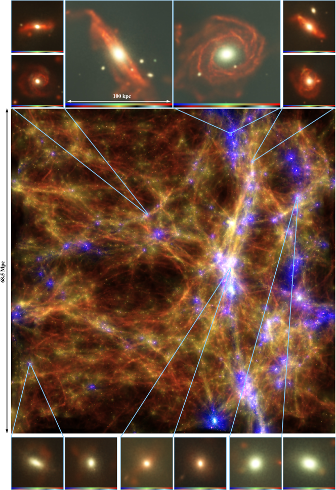
Figure 1.— Main panel: complete cosmological box at redshift $z=0.5$. The upper panels show exemplary spiral galaxies, and the lower panels show spheroidal galaxies. We show two random projection directions for each of the galaxies. In all panels we color-code the stellar particles by their cosmological formation epoch, where the upper color bars represent the age of the stars from old to young and the lower color bars represent the gas temperature from cold to hot. We also marked the position of the halos within the cosmological box.

Exemplary, Figure 1 shows six galaxies within the chosen mass range demonstrating that the galaxies in the simulations look like observed disk and spheroidal galaxies. The middle panel is a picture of the full cosmological box at redshift $z=0.5$.

3.1. The Angular Momentum

The mass and the angular momentum of galaxies are observed to be closely correlated with their morphology (e.g., Fall, 1983; Romanowsky & Fall, 2012; Obreschkow & Glazebrook, 2014). In a closed system without external forces, the angular momentum is a conserved quantity. However, in the context of galaxy formation and the interaction between collapsing objects and the large-scale structure, the assumption of the conservation is not necessarily fulfilled for a single galaxy. The total angular momentum of a galactic halo is given by

$$\textbf{J}=\sum_{k}\left(\sum_{i\in N_{k}}m_{k,i}\>\textbf{r}_{k,i}\times\textbf{v}_{k,i}\right),$$ (2)

where $k$ are the different particle types of our simulation (gas, stars, and DM) and $N_{k}$ is their corresponding particle number with the loop index $i$.

In our simulations, each particle carries its own mass. The initial mass is different for gas, star, and DM particles. Later on, the mass of individual gas particles varies owing to mass losses during star formation. Thus, we remove the mass dependence and use the specific angular momentum

$$\textbf{j}_{k}=\frac{\sum_{i}m_{k,i}\textbf{r}_{k,i}\times\textbf{v}_{k,i}}{\sum_{i}m_{k,i}},$$ (3)

where $k$ are the species of matter, as above. Therefore, we firstly calculate the angular momentum of each particle of a species. Afterward, we sum over all individual particles and divide by the total mass of the corresponding species to obtain the absolute value.

3.2. The Spin Parameter $\lambda$

In the following section we want to study the dimensionless $\lambda$-parameter. As defined by Peebles (1969, 1971) and adopted by, e.g., Mo et al. (1998), the general $\lambda$-parameter, which is used for the total halo, is given by

$$\lambda=\frac{J|E|^{1/2}}{GM^{5/2}},$$ (4)

where $E=-GM^{2}/2\>R_{\mathrm{vir}}$ is the total energy of the halo. This total spin parameter can only be used considering all matter inside the halo. To evaluate the different components (gas, stars, and DM), this parameter needs to be modified. We follow Bullock et al. (2001), who defined a component-wise spin parameter as follows:

$$\lambda^{\prime}(r):=\frac{J(r)}{\sqrt{2}M(r)V_{\mathrm{circ}}(r)r},$$ (5)

where $J(r)$ is the angular momentum, $M(r)$ the mass, and $V_{\mathrm{circ}}=\sqrt{GM(r)/r}$ the circular velocity within a radius $r$. Another advantage of $\lambda^{\prime}(r)$ is that it can be used for the calculation at different radii. When calculated over the entire virial radius, $\lambda^{\prime}(r)\approx\lambda$. For simplicity we will drop the prime for the remaining part of our study. For the evaluation of the different components $\lambda$ can be expressed in terms of the specific angular momentum, as done by van den Bosch et al. (2002):

$$\lambda_{k}=\frac{j_{k}}{\sqrt{2}R_{\mathrm{vir}}V_{\mathrm{circ}}},$$ (6)

where $k$ stands for the different components.

Independent of the definition, the distribution of the $\lambda$-parameter can be fitted by a lognormal distribution of the following form:

$$P(\lambda)=\frac{1}{\lambda\sqrt{2\pi}\sigma}\>\mathrm{exp}{\left(-\frac{ln^{2}(\lambda/\lambda_{0})}{2\sigma^{2}}\right)},$$ (7)

with the fit parameter $\lambda_{0}$, which is about the median value, and the standard deviation $\sigma$.

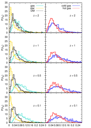
Figure 2.— Left panels: histograms for the $\lambda$-parameter for the different components within $R_{\mathrm{vir}}$; the DM (black) is the dominant component, the stars (yellow) peak at lower values, whereas the gas (turquoise) is distributed around higher values. While $\lambda_{0}$ stays relatively constant for the DM and stellar component, it increases for the gas with decreasing redshift. Right panels: the gas component splits into hot (red) and cold (blue) gas. Both components spin up with cosmic time, whereas for the cold gas this happens faster. Overplotted are the best-fit lognormal distributions (smooth lines), for which the parameters are reported in Table 1.

The left panels of Figure 2 show the histograms of the $\lambda_{k}$-distribution in linear bins of all halos in the selected mass range for stars (yellow), DM (black), and gas (turquoise) from redshift $z=2$ (upper panels) to $z=0.1$ (lower panels). The histograms and fit curves (smooth lines) are each normalized to the number of halos. The distribution of spin parameters of the stellar component has significantly lower values compared to the distribution of the spin parameter for DM, in agreement with the results presented by Danovich et al. (2015). This is due to the fact that within the halo the stars are more concentrated toward the center, whereas the spin of the DM component is dominated by the outer part of the halo, where most of the angular momentum of the DM component resides, as also shown in the right panel of Figure 22 in Appendix . In addition, major mergers result in a reduction of the specific angular momentum, as shown in Welker et al. (2014). On the contrary, the gas component always has a spin parameter distribution shifted toward larger values, in agreement with more recent studies by Sharma & Steinmetz (2005), Kimm et al. (2011), Sharma et al. (2012), and Danovich et al. (2015), but in contrast to previous studies by van den Bosch et al. (2002) and Chen et al. (2003), who found nearly the same spin distributions for gas and DM. The larger spin values for the gas reflect the continuous transport of the larger angular momentum from the outer parts into the center due to gas cooling. While this leads even to a spinning up of the gas component with time, the distributions for the stars and DM remain relatively constant. This spin-up of the gas component might be caused by the continuously accreted cold gas, which brings in large angular momentum from farther away along the filaments (Pichon et al., 2011). When dividing the gas into hot and cold phases, we note that the hot gas (red) has lower values than the cold gas (blue), which has a long tail to high $\lambda$-values. This is in contrast to Chen et al. (2003), who found that the spin parameter for the hot gas is higher than that of the cold gas. On the other hand, our results agree well with more recent studies by Danovich et al. (2015). This trend for the cold gas to high values was also seen by Stewart et al. (2011), who have calculated $\lambda$-values for the cold gas and found values around $0.1-0.2$. For a better overview we have listed the fit value of the $\lambda$-distribution for the different components in Table 1.

Table 1The $\lambda_{0}$ Fit Value for the Different Components at Different Redshifts

Redshift	$\lambda_{\mathrm{stars}}$	$\lambda_{\mathrm{DM}}$	$\lambda_{\mathrm{gas}}$	$\lambda_{\mathrm{hot}}$	$\lambda_{\mathrm{cold}}$
2	0.023	0.043	0.061	0.053	0.074
1	0.026	0.046	0.078	0.069	0.097
0.5	0.021	0.042	0.085	0.078	0.107
0.1	0.020	0.042	0.090	0.083	0.123

3.3. Alignments

In this subsection we want to study the orientation of the angular momentum vectors of the different components in comparison to each other within the innermost region of the halo. For the calculation of the innermost region of the halo we only take particles within the inner 10% of the virial radius ($R_{\mathrm{vir}}$) into account, which corresponds roughly to the size of the galaxies. We chose this radius as an approximate medium value, since smaller disks have a size of about 5% while extended gaseous disks can reach out up to 20% of the virial radius.

The angle between two vectors of the species $i$ and $j$ is calculated by

$$\mathrm{cos}\left(\theta\right)=\frac{\textbf{J}_{i}\cdot\textbf{J}_{j}}{|\textbf{J}_{i}|\cdot|\textbf{J}_{j}|}.$$ (8)

We then bin the angles from 0 to 180 degrees in 18 bins of a size of $10^{\circ}$ each and count the number of halos within each bin. For the plots the number is normalized to unity.

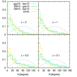
Figure 3.— Angle between the total angular momentum vectors of the different components within the innermost 10% of $R_{\mathrm{vir}}$ as indicated in the plots for different redshifts. The gray dot-dashed line is expected for a random distribution of the angles. At higher redshift the gas and stellar components (green dotted) are well aligned, and their alignment gets worse with decreasing redshift. In contrast, the alignment of the DM and the stars (yellow dashed) gets better with decreasing redshift.

As shown in Figure 3, the distribution of the angles between the angular momentum vectors of gas and stars (green dotted) generally shows a good alignment at higher redshifts and becomes less aligned with decreasing redshift. This is in contrast to the alignment between the DM and stellar components (yellow dashed), which shows a better alignment with decreasing redshift. The angles between the DM and the gas component (turquoise solid) are an intermediate case, and their distribution does not change with redshift. For comparison, a random distribution of alignment angles is shown as a gray dot-dashed line in Figure 3, demonstrating that none of the angle distributions found in the simulations are of random nature. The difference between the behavior and especially the evolution of the alignment of the gas and the stellar component can be explained by the fact that the angular momentum of the gas reflects the freshly accreted material (similar to the stars at high redshift), while the stars at low redshift reflect the overall formation history, similar to the DM content. These trends are in qualitative agreement with results obtained from simulations at very high redshift ($z>9$) by Biffi & Maio (2013), who also found the angular momentum of the gas component in the center to reflect the recent accretion history.

4. Kinematical Split-Up

In this section we investigate properties of our galaxies as a function of their stellar mass and angular momentum. We therefore calculate the angular momentum J of the stars within the innermost 10% of the virial radius. Furthermore, we ignore all particles within the innermost 1% of the virial radius because of their potentially unknown contributions caused by bulge components or numerical resolution effects. We rotate the positions and velocities of all particles such that their $z$-components are aligned with the angular momentum vector J of the stellar component. In the same manner we produce another data set that is rotated such that the $z$-components are aligned with the angular momentum vector J of the gas component. These data are used for the $\varepsilon_{\mathrm{gas}}$-distribution because the gas circularity calculated with the data rotated according to the angular momentum of the stars can fail to detect a gas disk that is misaligned with the stellar disk and vice versa.

4.1. The Circularity Parameter $\varepsilon$

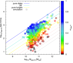
Figure 4.— Stellar mass in the inner 10% of the virial radius vs. the specific angular momentum of the stars for all halos at redshift $z=0.1$. The mean circularity $\varepsilon_{\mathrm{star}}$ of the halos is color-coded. We adopted the scaling relations of Romanowsky & Fall (2012) (their Figure 2), where the blue line stands for pure disks, the turquoise one for S0, and the yellow one for pure bulges.

Since in the Magneticum simulations disk and spheroidal galaxies are formed, we need to categorize them for our analysis according to their morphology. In order to distinguish between different types of galaxies, we use the circularity parameter $\varepsilon$. The $\varepsilon$-parameter was first introduced by Abadi et al. (2003) as $\varepsilon_{J}=J_{z}/J_{\mathrm{circ}}(E)$. For our study we use the definition of Scannapieco et al. (2008), which is given by

$$\varepsilon=\frac{j_{z}}{j_{\mathrm{circ}}}=\frac{j_{z}}{rV_{\mathrm{circ}}},$$ (9)

where $j_{z}$ is the $z$-component of the specific angular momentum of an individual particle and $j_{\mathrm{circ}}$ is the expected specific angular momentum of this particle assuming a circular orbit with radius $r$ around the halo center of mass, with an orbital velocity of $V_{\mathrm{circ}}(r)=\sqrt{GM(r)/r}$.

We compute the circularity $\varepsilon$ for every individual particle between 1% and 10% of the virial radius. This is done for the stellar and the gas component, where we use the data that were rotated according to the angular momentum of the stars or the gas, respectively. To obtain the circularity distribution for our selected halos, we compute the fractions $f(\varepsilon)$ of particles within equal-distant bins, using a bin size of $\Delta\varepsilon=0.1$. In a dispersion-dominated system there is usually a broad peak in the distribution at $\varepsilon\simeq 0$, while in a rotation-supported system there is usually a broad peak at $\varepsilon\simeq 1$.

To test the hypothesis that the mass and the angular momentum of galaxies are the most important ingredients in their formation history and the resulting morphology (e.g., Fall, 1983; Romanowsky & Fall, 2012; Obreschkow & Glazebrook, 2014), we plot our galaxies at $z=0.1$ in the stellar mass vs. stellar angular momentum plane in Figure 4. Thereto we take all star particles within the innermost 10% into account. We color-code the simulated galaxies according to the absolute value of the mean of their stellar circularity parameter. Adopting the classification diagram of galaxies by Romanowsky & Fall (2012) (their Figure 2), we overplot lines where the specific angular momentum follows the relation $j\propto M^{\alpha}$ with $\alpha\approx 2/3$. We plot different lines with distance $\Delta b=0.25$. As can clearly be seen in Figure 4, the mean circularity parameter is following this relation. Inspired by this result, we classify our galaxies according to what we will in the following refer to as the “$b$-value”:

$$b=\mathrm{log}_{10}\left(\frac{j_{\mathrm{star}}}{\mathrm{kpc}~{}\mathrm{km/s}}\right)-\frac{2}{3}\mathrm{log}_{10}\left(\frac{M_{\mathrm{star}}}{M_{\odot}}\right),$$ (10)

which is the $y$-intercept of the linear relation $f(x)=ax+b$ in the log-log of the stellar-mass–specific-angular-momentum plane.

According to Romanowsky & Fall (2012), galaxies with $b$-values close to $-4$ (blue line) are expected to be disks, while $b\approx-5$ indicates pure spheroidals (yellow). In our simulations we even find galaxies with $b$-values down to $b=-6.25$ for the galaxies with the smallest specific stellar angular momentum.

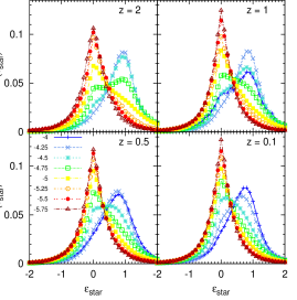
Figure 5.— Averaged $\varepsilon$-distributions of the stellar component for four redshifts. Thereby, each $\varepsilon$ bin is averaged over all halos that lie in the corresponding $b$-value bin. We see a clear transition of the galaxy types from rotational-supported systems to dispersion-dominated systems at all redshifts.

Figure 5 shows the averaged $\varepsilon$-distribution of the stellar component at four redshifts, colored according to the different $b$-value bins shown in Figure 4. Each $\varepsilon$ bin is averaged over the halos that reside in the chosen $b$-value bin. There is a clear transition between the galaxies with different dynamics, from rotational-supported ($\langle\varepsilon\rangle=1$) to dispersion-supported ($\langle\varepsilon\rangle=0$) systems, reflected by their $b$-value from the $M_{\mathrm{star}}$-$j_{\mathrm{star}}$-plane: While galaxies with $b\approx-4$ clearly have most stars around $\varepsilon=1$, and thus are dominated by rotation, galaxies with $b\approx-6$ peak around $\varepsilon=0$, indicating that there is no significant rotation. This is true for all redshifts. However, we see a slight trend with redshift at intermediate $b$-values: for example, the distribution of the halos in a $b$-value bin of $-4.75$ (green squares) at $z=2$ has the higher of the two peaks around $\varepsilon=1$, whereas at $z=0.1$ it only peaks around $\varepsilon=0$. It is also interesting that the galaxies in the $b$-value bin of $-4.5$ (turquoise stars) at redshift $z=2$ have a dominant rotationally ordered component, which becomes more dispersion dominated with decreasing redshift. We also note that the distributions around $\varepsilon=0$ become slightly more distinct at lower redshifts. This indicates that there is an evolution of the different galaxy types with cosmic time along the $M_{\mathrm{star}}$-$j_{\mathrm{star}}$-plane.

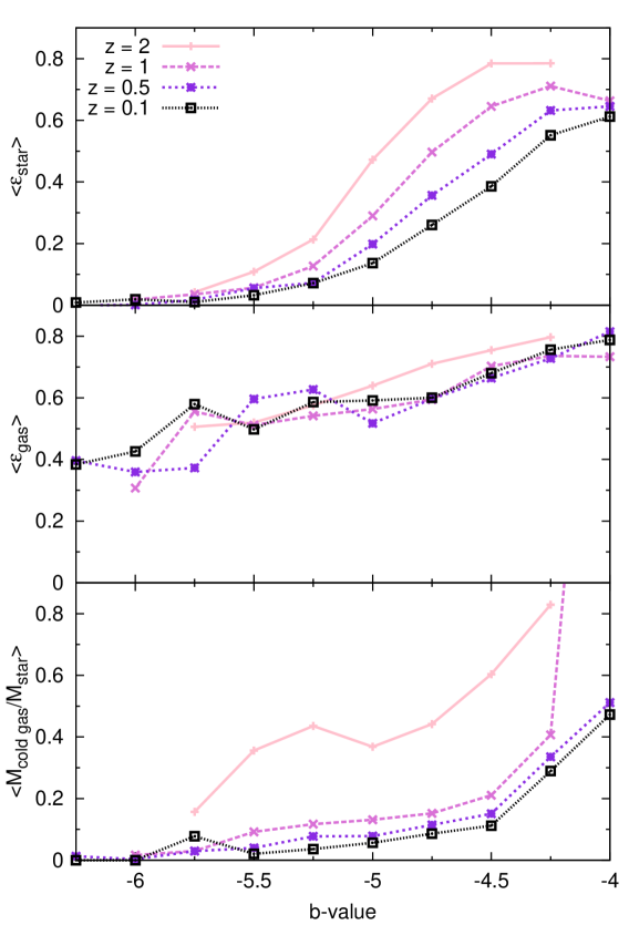
Figure 6.— Top: mean circularity $\varepsilon$ of the star component averaged over all halos in the corresponding $b$-value bin. There is a clear trend for decreasing mean $\varepsilon$ when moving from the pure disks (high $b$-value) down to the pure bulges (smaller $b$-value) for all four redshifts. Middle: same as the top panel, but for the $\varepsilon$ of the gas component. Bottom: The mass fraction of cold gas with respect to the stars, both within the inner 10% of the virial radius, averaged over all halos in the corresponding bin. At high redshift (pink solid line) there is much more cold gas, even in halos with a smaller $b$-value.

This additional evolutionary trend gets more evident in Figure 6, which shows $\varepsilon_{\mathrm{star}}$ (top), $\varepsilon_{\mathrm{gas}}$ (middle), and the mass fraction of the cold gas with respect to the stellar mass (bottom) versus the $b$-value, with spheroidal systems at the left and disk-like systems on the right. Thereby, each of these properties is averaged over the halos in the corresponding $b$-value bin. We can clearly see that the average $\varepsilon_{\mathrm{star}}$ increases with increasing $b$-value at all four redshifts. Additionally, the average stellar circularity is generally larger at higher redshifts for all types of galaxies, albeit this trend is stronger for galaxies with larger $b$-values. This clearly shows that disk galaxies at higher redshifts had less prominent central bulges that would shift the value toward $\langle\varepsilon\rangle=0$. For $\langle\varepsilon_{\mathrm{gas}}\rangle$ we do not find any clear trend. The bottom panel of Figure 6 shows a similar trend for the mean cold gas fraction. The spheroidal systems at present day with small $b$-values have only low amounts of gas, compared to the stellar mass, usually below 10%, whereas disks have gas fractions of 20% or more. For higher redshifts this fraction increases successively, and the strongest evolution is visible between redshifts $z=2$ (pink solid line) and $z=1$. Below $z=1$ there is only a mild but continuous evolution, but at $z=2$ even spheroidals have gas fractions of 20% or more, while disk galaxies can contain more than 40% gas compared to their stellar content. For the largest $b$-values the galaxies can even be dominated by gas, i.e., the gas fraction is larger than 50%. Thus, we conclude also that galaxies that are spheroidal systems have a nonnegligible cold gas fraction at high redshifts.

4.2. The $\lambda$-parameter

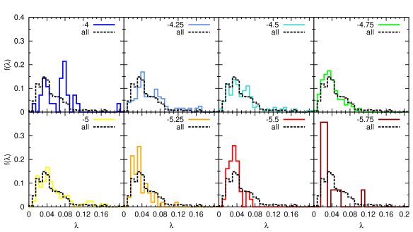
Figure 7.— Distribution of the total $\lambda$-parameter for the halos according to their $b$-values at $z=0.1$. There is a transition from the disks (upper left) to the bulges (lower right), i.e., from rotation-dominated systems (higher $\lambda$-values) to dispersion-dominated systems (lower $\lambda$-values). Interestingly, the halos with the highest $b$-values show a dichotomy in their distribution.

We want to understand whether this classification of the galaxies according to their position on the $M_{\mathrm{star}}$-$j_{\mathrm{star}}$-plane has an effect on the spin parameter $\lambda$. In Figure 7 we show the distribution of the total $\lambda$-parameter of the whole halo content (see Equation 4), exemplary for redshift $z=0.1$. We divide the halos according to their $b$-value. The first interesting thing to note is that there is a double peak in the $\lambda$-distribution for galaxies with disk-like kinematics (upper left panel). This could indicate that there are different formation channels for disk-like systems, e.g., gas-rich major mergers, as discussed in Springel & Hernquist (2005) and Schlachtberger, D.P. (2014). The peak at higher $\lambda$-values becomes smaller as we move to the right and seems to disappear at a $b$-value of $-4.75$. Galaxies with $b$-values below $-5.25$ are hosted in halos with significantly smaller $\lambda$-values compared to the overall distribution (black dashed line). Therefore, on average there seems to be a connection between the galaxy types and the spin parameter $\lambda$ of the hosting halos, reflected in a continuous transition of the spin parameter distribution of the host halo with the $b$-value obtained from the $M_{\mathrm{star}}$-$j_{\mathrm{star}}$-plane.

4.3. Alignments of the Central Components

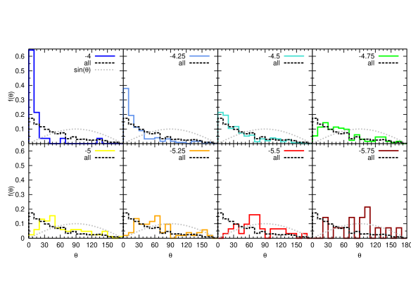
Figure 8.— Angle between the angular momentum vector of the gas and that of the stars within the innermost 10% of the virial radius according to their $b$-values at redshift $z=0.1$. There is a clear transition between the galaxy types. The higher the $b$-value, the better aligned the stellar and gas components are. When going to lower $b$-values, i.e., moving down on the $M_{\mathrm{star}}$-$j_{\mathrm{star}}$-plane to the bulges, the angles of the two components seem to be randomly distributed (compare gray dotted sinusoidal distribution).

To verify the dynamical connection between the different baryonic components within the galaxies, we show in Figure 8 the distributions of the alignment between the central angular momentum of the stellar and the gas component. As before, we classify our galaxies according to the $b$-value. By moving from high (upper left) to low (lower right) $b$-values we immediately see that the alignment between the angles is good for the disk galaxies (large $b$-values) and gets increasingly more random for decreasing $b$-values. This is indicated by the gray dotted line, which again illustrates a random distribution (as in Figure 3). We find a continuous transition from the disk-like to the bulge-dominated galaxies. It illustrates that in spheroidal systems the stars are significantly misaligned with an eventually present gaseous disk. This result is supported by the findings of the $\mathrm{ATLAS^{3D}}$-project (Cappellari et al., 2011) that a kinematical misalignment of the gas component with respect to the stars is not unusual (Davis et al., 2011).

5. Classification of Simulated Galaxies

So far we have seen that there is a continuous transition between the different types of galaxies within the $M_{\mathrm{star}}$-$j_{\mathrm{star}}$-plane, orthogonal to $j\propto M^{\alpha}$ with $\alpha\approx 2/3$. We now want to study the kinematical properties of our simulated galaxies depending on their classification as disk and spheroidal galaxies.

5.1. Selection Criteria

In our simulations, many spheroidal galaxies show extended, ring-like structures of cold gas, in good agreement with recent observations (Salim & Rich, 2010). Therefore, including the circularity of the gas within 10% of the virial radius as a tracer of morphology can lead to a misinterpretation. Additionally, there can be huge uncertainties for galaxies that have almost no gas left. Using a criterion only based on the $b$-value of the galaxies also is not straightforward because of the existence of fast rotators among the spheroidal galaxies. Observationally there seems to exist some overlap between the different galaxy types within the $M_{\mathrm{star}}$-$j_{\mathrm{star}}$-plane. In principal, the luminosity of the stars could be taken into account, since old stars that make up the bulge and the halo stars are not as luminous as young stars that build up the disk. Hence, in observations a galaxy with an old massive stellar bulge and an extended disk of young stars and gas is very likely to be classified as a spiral galaxy.

However, here we will stick to a classification of galaxies based on the circularity distribution (Equation 9) of their stars, which allows us to capture rotationally supported stellar disk structures or dispersion-dominated spheroidal structures. We combine this criterion with the mass fraction of the cold gas with respect to the stars, following our result from Figure 6. As before, circularity distributions are evaluated within 10% of the virial radius, excluding the central 1%, while we include the central 1% in our calculation of the cold gas fraction as the resolution is not important in this case. We use the results from the previous section to justify the threshold values used to select dispersion-dominated, gas-poor spheroidal and rotational-supported, gas-rich disk galaxies to reflect counterparts of classical, observed elliptical, and spiral galaxies.

As shown in Figure 5, there is a clear, bimodal behavior of the epsilon distribution within different $b$-value bins. We show in Appendix in detail the cumulative distributions that allow us to define the proper thresholds bracketing the transition regions. These thresholds are then applied to the circularity distributions of the individual galaxies, which of course in general show a more complex shape than the averaged distributions. The left panel of Figure 20 in Appendix shows the cold gas mass fraction of the galaxies classified only by their circularity $\varepsilon_{\mathrm{star}}$, illustrating our choice of including a gas criterion. In short, we are using the following selection criteria:

• We classify a galaxy as a spheroidal galaxy if the majority of particles is in a close interval around the origin (i.e., $f(-0.4\leq\varepsilon\leq 0.4)\geq 0.6$). This percentage cut is adapted to the redshift. For the details see the left panels of Figure 19 in Appendix .

  In addition, it has to have a cold gas mass fraction with respect to the stars lower than $0.35$ at $z=2$, $0.2$ at $z=1$, $0.125$ at $z=0.5$, and $0.065$ at $z=0.1$. This criterion is chosen such that the fraction values satisfy the linear function $f(z)=0.15\cdot z+0.05$. The upper limit for the spheroidal galaxies at redshift $z=0.1$ seems plausible, since Young et al. (2014) found that massive elliptical galaxies (of the red sequence) have mass fractions of $HI$ and $H_{2}$, compared to the stars, up to 6% and 1%, respectively.

• We classify a galaxy as a disk galaxy if the majority of particles are off-centered from the origin (i.e., $f(0.7\leq\varepsilon\leq 3)\geq 0.4$; for the dependence on the redshift see right panels of Figure 19 in Appendix ).

  Additionally, the constraint on the mass fraction of the cold gas is such that it has to be higher than $0.5$ at $z=2$, $0.35$ at $z=1$, $0.275$ at $z=0.5$, and $0.215$ at $z=0.1$. This criterion is chosen such that the values of the mass fraction satisfy the linear function $f(z)=0.15\cdot z+0.2$.

• All remaining galaxies, which fulfill neither of the two criteria, are classified as “others.”

The total number of galaxies above the mass cut of $5\cdot 10^{11}M_{\odot}$ selected from our simulation at redshift $z=0.1$ is 622 (for other redshifts see Table 2). According to the above criteria, 64 galaxies are classified as classical disks and 110 as classical spheroids, while 448 are classified as “others.” Such unclassified galaxies include merging objects, bulge-dominated spirals, spheroids with extended gas disks, barred galaxies, or irregular objects.

Table 2Number of Halos in the Selected Mass Range

Redshift	$N$	$N_{\mathrm{spheroid}}$	$N_{\mathrm{disk}}$
2	396	34	89
1	606	87	73
0.5	629	146	59
0.1	622	110	64

In order to identify parts of the unclassified objects, the classification could be refined in such a way that we additionally divide into spheroids that have a gaseous star-forming disk or galaxies that have a large stellar disk with only little gas (S0 galaxies). At lower redshifts our classification becomes increasingly difficult since there are a lot of galaxies that have a very dominant stellar bulge but, on the other hand, also possess an extended gaseous disk containing many young stars.

Although the criterion for the gas mass fraction is relatively arbitrary and may overestimate the number of spheroids, we checked that changing this selection criterion does not change the results qualitatively, although adding/removing galaxies from the spheroidal sample. At higher redshifts an additional difficulty might be that the transition of galaxy types is less strict, as seen in Figure 5. At these redshifts, remaining dynamical signatures of the current formation process will be more pronounced and individual distributions of the circularity parameter might be more complex. Thus, a clear assignment might fail.

5.2. Comparison of the Simulated Stellar Specific Angular Momentum with Observations

After having extracted a set of spheroidal and disk galaxies, we can evaluate the relation between the specific angular momentum and the mass of the stellar component and compare them with observations, as shown in Figure 9.

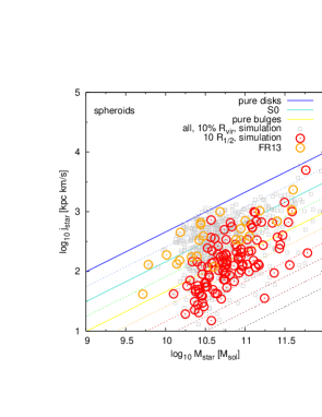
Figure 9.— Galaxies within the stellar-mass–specific-angular-momentum plane at $z=0.1$. Gray symbols represent all galaxies extracted from the simulations (as in Figure 4), where angular momentum and stellar mass are measured within 10% of the virial radius. The left panel shows the simulated galaxies classified as spheroids (red circles) compared to data from observed elliptical galaxies by Fall & Romanowsky (2013) (orange circles, denoted by “FR13”). The right panel shows disks in our simulation (blue diamonds) compared to observational data of spiral galaxies by FR13 (purple diamonds). For the disks and the spheroids, we evaluated the mass and the specific angular momentum within $10~{}R_{1/2}$, which more closely resembles the radii studied by FR13. The colored lines correspond to the $b$-values (see Figure 4).

To compare with observations presented by Fall & Romanowsky (2013) (hereafter FR13) we calculate the mass and specific angular momentum for all stellar particles within $10~{}R_{1/2}$ instead of $10\%R_{\mathrm{vir}}$, where $R_{1/2}$ is the radius that contains half the stellar mass of the galaxy and roughly corresponds to observed effective radii. This is done to account for the fact that, for a given mass, disk galaxies have a larger effective radius than spheroids (Shen et al., 2003), and to better resemble the radius ranges studied in FR13. The left panel shows the $M_{\mathrm{star}}$-$j_{\mathrm{star}}$-plane for our galaxies classified as spheroids (red circles), including the 23 elliptical galaxies (orange circles) presented in FR13 (their Figure 2). In the right panel the same is shown for our disk galaxies (blue diamonds) in comparison to the 57 spiral galaxies (purple diamonds) from FR13. In general, our simulated galaxies are in good agreement with the observations. This result has already been shown for a subset of our galaxies at $z=0$ with a rather crude classification criterion in Remus et al. (2015), and we find an even better agreement with observations with our more advanced classification scheme. Recently, Genel et al. (2015) have shown a comparison of the galaxies in the Illustris simulation with those observations, which are also in good agreement when a similar feedback mechanism is used.

To understand the impact of the choice of radius used to calculate the angular momentum and the stellar mass, we included the values for all galaxies evaluated within 10% of the virial radius, as previously shown in Figure 4. For the spheroidal galaxies the effect is much stronger, and we clearly see that the angular momentum is larger for larger radii. The radius dependence is shown in more detail in the right panel of Figure 22 in Appendix , where we show that the angular momentum of spheroids increases with radius and that there is a significant contribution to the specific angular momentum from large radii. For disk galaxies the exact radius is less important, as most of the angular momentum is contained within the disk at relatively small radii. The same holds true for the $b$-value, which more strongly depends on the considered radius for spheroids than for disks, which can be seen in Figure 23 in Appendix .

Note that we compare here the specific angular momentum directly measured from the total stellar component from the simulations (Equation 3), while the observations are inferred from the projected measurements. We also do not resolve galaxies with stellar masses smaller than $\approx 10^{10}M_{\odot}$, while the observations include some objects with smaller masses.

5.3. The Gas and Stellar Specific Angular Momentum in Simulations and Observations

We also compare the specific angular momentum of the gas with that of the stars for all classified galaxies in our simulations.

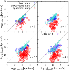
Figure 10.— Specific angular momentum of the gas against the specific angular momentum of stars, both within 10% of the virial radius for galaxies which are classified as disks (blue diamonds) at four redshifts as indicated in the plots. Additionally, we show the relation also considering only young stars (turquoise diamonds). At $z=0.1$ we overplot observational data points calculated by Obreschkow & Glazebrook (2014) (purple pentagons). The values agree well with the observations, and we note an overall spin-up with cosmic time.

Figure 10 shows the relations for all four redshifts as indicated in the plots. At redshift $z=0.1$ we include the observational data taken from the THINGS (The HI Nearby Galaxy Survey, Walter et al., 2008) sample, which consists of 16 spiral galaxies in the local Universe, for which surface densities of stars and cold gas are available (Leroy et al., 2008). Specific angular momenta for the gas and stellar components of those galaxies were presented by Obreschkow & Glazebrook (2014).

For the disk galaxies, we find that the specific angular momentum of all stars in the central region is slightly smaller than that of the gas (blue diamonds), in agreement with the observations (purple symbols). This, most likely, originates from the fact that the specific angular momentum of the gas is constantly replenished by freshly accreted gas, which transports larger angular momentum from the outer parts of the halo to the center. This becomes more evident by looking at the newly formed stars (turquoise diamonds) in our simulations. We consider a star to be young if its formation happened not more than $\Delta z=0.05\times 1/(1+z)$ ago at a given redshift $z$, which corresponds to a stellar age of $0.2\mathrm{Gyr}$ at $z=2$, $0.4\mathrm{Gyr}$ at $z=1$, $0.5\mathrm{Gyr}$ at $z=0.5$, and $0.7\mathrm{Gyr}$ at $z=0.1$. If we only take the young stars into account, we find almost an equality (dotted line) with the specific angular momentum of the gas. At a lower redshift (lower right panel) the values of the specific angular momentum of the gas are slightly larger than at higher redshift (upper left panel). This behavior reflects the spin-up of the cold gas with time, as already seen before. Hence, also the young stars have higher specific angular momentum. This appears in a slight trend for a separation of the young stars and the total stellar component, which have lower specific angular momentum than the gas.

The spheroids (red circles in Figure 10), however, have a significantly lower specific stellar angular momentum compared to that of their gas. This suggests that, especially at high $z$, most gas in spheroids originates from the accretion of material from large radii (cold streams or infalling substructures) and hence transports the higher angular momentum from the outer parts into the center.

We can clearly see that the spheroids and the disk galaxies show a different behavior in the relation between the angular momentum of the gas and stars. We also have seen that the gas gains angular momentum over time, especially in disk galaxies. In disk galaxies, stars have slightly smaller specific angular momentum than the gas, and they also show a mild difference between the specific angular momentum of stellar components with different ages. Here the young stars have slightly larger specific angular momentum, basically reflecting the angular momentum of the gas from which they form.

All in all, the results from the simulations fit well with the observational data. In particular, we are in agreement with Fall (1983), who find that the specific angular momentum of the galaxies increases with the disk-to-bulge ratio for a given mass.

We note that the evaluation of this quantity for spheroids especially at lower redshifts might be fault-prone since, owing to the selection criterion, there is only a small amount of cold gas within the chosen radial range.

5.4. Comparison of the Gas and DM Specific Angular Momenta

Finally, we compare the specific angular momenta of DM and gas. In particular, we are interested in the scaling relations of the corresponding individual specific angular momenta of baryonic and nonbaryonic matter. Previous studies (e.g., Fall, 1983; Mo et al., 1998) suggest an equality between the angular momentum of the total DM halo and that of the central gas component of disk galaxies.

The relation between the specific angular momentum of the cold gas of the galaxy, which resides within the innermost 10% of the virial radius, and that of the total DM halo is shown in Figure 11 for different redshifts. In general, we find the specific angular momentum of the DM to exceed (by a factor of $\approx 2$) the specific angular momentum of the cold gas. Interestingly, the cold gas in disk and spheroidal galaxies does behave in the same way. This is due to the fact that cold gas always settles in disk-like structures, even in elliptical galaxies (e.g., Lees et al., 1991; Young et al., 2011). We plot all disks above the redshift-dependent $M_{\mathrm{cold}}/M_{\mathrm{star}}$-cut (blue diamonds). Additionally, we fit a line parallel to the 1:1 relation (blue dotted) to the data, in order to see the offset. For all shown redshifts we find values of the $y$-intercept between $0.33$ and $0.41$ in log space, which is between $2.14$ kpc km/s and $2.57$ kpc km/s in normal space. However, the scatter around this fit curve is very large. The yellow diamonds show the value for one simulated galaxy at different redshifts as presented in Kimm et al. (2011). Their disk galaxy has only slightly higher specific angular momentum in the gas component compared to the DM halo, but sits within the distribution of values we find in our simulation for different galaxies. Our values are also broadly in line with the results of Danovich et al. (2015), who find that the spin of the disk is comparable to that of the DM halo. The size of the symbols of the spheroids (red circles) is plotted according to their fraction of cold gas mass with respect to the stellar mass. For completeness we plot all spheroids with a cold gas mass fraction lower than 35% for all redshifts. At higher redshift most spheroids have a large amount of cold gas. At the lowest redshift there are still some objects that were classified as spheroids with the $\varepsilon_{\mathrm{star}}$-criterion but have a high cold gas mass fraction. Interestingly, there are some spheroids with high specific cold gas angular momentum, which might be due to individual infalling clumps and small substructures, as these are spheroidal galaxies that have extremely small cold gas fractions. However, in such cases we cannot relate the specific angular momentum of these individual structures to the specific angular momentum of the halo.

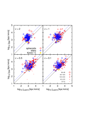
Figure 11.— Specific angular momentum of the cold gas within 10% of the virial radius against the specific angular momentum of DM within the entire virial radius. The blue diamonds show the disks and the red circles the spheroidal galaxies, where the size of the circles reflects the fraction of the cold gas mass with respect to the stellar mass. The blue dotted line shows the fit for the disk galaxies. The 1:1 relation is represented by the black dashed line. For comparison, we add the results obtained by Kimm et al. (2011) (yellow diamonds).

5.5. Misalignment Angles

As seen before, another indicator for the different evolutionary states reflected by the stars, DM, and gas are the misalignment angles between these three components. We now investigate their behavior by focusing on our selected disk and spheroidal galaxies.

5.5.1 The Angle between Gas and Stars

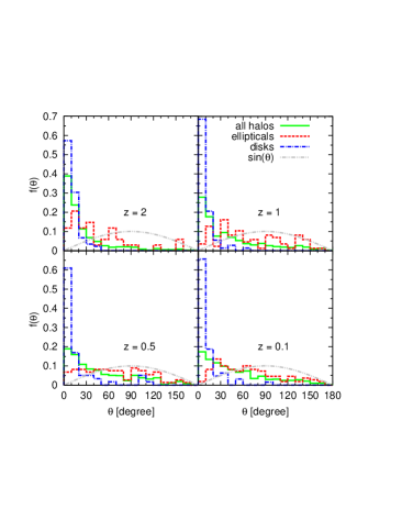
Figure 12.— Angle between the angular momentum vector of gas and stars, both within the innermost 10% of the virial radius. At all redshifts the disks (blue dot-dashed) are well aligned. In contrast, the spheroids (red dashed) are randomly distributed. The overall distribution (green solid) gets worse aligned with decreasing redshift.

At first, we investigate whether we find a correlation between the morphological type and the angles between the angular momenta of the gas and the stars, both within the innermost 10% of the virial radius. Figure 12 shows the angle for four different redshifts. The disk galaxies (blue dot-dashed histograms) have very well aligned gas and stellar angular momentum vectors with median values of $7.8^{\circ}$ at redshifts $z=2$ and $z=0.1$ and median values of $6.3^{\circ}$ and $7.6^{\circ}$ at redshifts $z=1$ and $z=0.5$, respectively. This is in good agreement with Hahn et al. (2010), who found median angles of about $8^{\circ}$ for their disks at $z=1$ and a median of $7^{\circ}$ at redshifts $z=0.5$ and $z=0$. It demonstrates that the stellar and gaseous disks in disk galaxies are very well aligned, which is what we expect, since the stars form out of the gas and thus maintain the same orientation.

The spheroids have a random distribution with a median value of $60.4^{\circ}$, i.e., the gas and stellar components in spheroidal galaxies are often misaligned. In summary, the gas and star components of spheroids become less aligned with decreasing redshift, while there is no change for disk galaxies (see Table 3). The overall trend for all halos in the simulation shows the same behavior as the spheroids, in agreement with Figure 8.

Table 3Median Misalignment Angles between the Baryons in the Center

Redshift	All Halos	Disks	Spheroids
2	13.4	7.8	37.4
1	24.4	6.3	56.5
0.5	35.8	7.6	65.5
0.1	37.6	7.8	60.4

5.5.2 The Angle between DM and Baryons

Figure 13.— Left: angle between the total angular momentum vector of DM in $R_{\mathrm{vir}}$ and the gas within the innermost 10% of $R_{\mathrm{vir}}$. The overall alignment is poor. Middle: The angle between the total angular momentum vectors of the DM and stars within $R_{\mathrm{vir}}$. The disk galaxies (blue dot-dashed lines) seem significantly better aligned than the spheroids (red dot-dashed lines). Right: angle between the total angular momentum vector of the DM in $R_{\mathrm{vir}}$ and the stars within the innermost 10% of the virial radius. For all shown distributions the alignment is very poor, almost random.

Since we see a clear difference in the alignment between the angular momenta of the stars and gas for spheroids and disks, we want to test whether this is reflected in the relation between the angular momentum of the baryonic components and DM. The left panel of Figure 13 shows the misalignment angle between the angular momentum of the total DM halo and the gas within the inner 10% of the virial radius at redshift $z=0.1$. Again, the gray dashed line is the expected distribution if the angles were spread randomly. We clearly see that the median misalignment found for all halos (green solid lines) is $\approx 49^{\circ}$, for the disks $\approx 45^{\circ}$, and for the spheroids $\approx 47^{\circ}$. This is slightly larger than the results of Sharma et al. (2012), who found a median misalignment angle of about $30^{\circ}$ for the gas within the innermost 10% of the virial radius compared to the total angular momentum vector of all halos. On the other hand, Hahn et al. (2010) compared the angular momentum of the gas component of the disk to the total angular momentum and obtained about $49^{\circ}$ at $z=0$, well in line with our results.

We now want to see under which circumstances the orientation of the angular momentum vectors of the total DM halo is reflected in that of the stellar component, since we have seen in Figure 12 that the angular momentum vectors of the gas and that of the stars are very well aligned in the inner part of the halo for disk galaxies and poorly aligned for spheroids. The angle between the angular momentum vectors of the DM and that of the stars within the virial radius is shown in the middle panel of Figure 13. In general, there is an alignment of the two components. The disk galaxies are slightly better aligned with a median angle of $\approx 18^{\circ}$ compared to the spheroids that have a median angle of $\approx 31^{\circ}$. As a median value for all halos we find $\approx 24^{\circ}$ at redshift $z=0.1$ and a similar value for $z=1$, namely, $\approx 22^{\circ}$, which is not shown here.

The right panel of Figure 13 shows the angle between the angular momentum vector of the stars within the inner 10% of the virial radius and the DM within the entire virial radius. The distribution of the alignment angles looks similar to that of the gas (left panel of Figure 13) for all galaxies. The alignment seems poor, with median angles of $\approx 55^{\circ}$ for all halos, $\approx 46^{\circ}$ for disks, and $\approx 57^{\circ}$ for spheroidal galaxies. This agrees well with Hahn et al. (2010), who calculated a median angle of the stellar component and the total halo content of about $\approx 49^{\circ}$ at $z=0$ for disk galaxies, similar to Croft et al. (2009) reporting a median angle of $\approx 44^{\circ}$ at redshift $z=1$. Bett et al. (2010) found slightly smaller angles of $\approx 34^{\circ}$ for the alignment of the galaxies with respect to the hosting total DM halo. The galaxies at $z=1.2$ investigated by Codis et al. (2015), using the Horizon-AGN simulation, are slightly less aligned with their DM halos than our simulated galaxies (see also the right panel of Figure 20 of Appendix ). Deason et al. (2011) reported that 41% of their disk galaxies had misalignment angles larger than $45^{\circ}$ with their DM halo. In addition, they found that the disk galaxies are better aligned with the DM in the innermost 10% of the $r_{200}$. Though we do not show this, here we obtained a median angle of $\approx 9^{\circ}$ for the angular momentum vectors of the stellar and DM components in the innermost 10% for our disk galaxies at $z=0.1$, and thus we can confirm this trend. It also agrees well with Hahn et al. (2010), who find a median value of $\approx 15^{\circ}$ for the angle between the DM and stellar components of the galactic disks. For the DM and the gaseous components of their disks they obtain a median value of $\approx 18^{\circ}$, which is in line with the median value of $\approx 12^{\circ}$ for our disk galaxies.

6. The Host Halos of Different Galaxy Types

So far we have seen the intrinsic difference of the baryonic components and how they reflect global halo properties for galaxies classified as either disk or spheroidal galaxies. We now want to study whether there are underlying differences in the DM halo contributing to the formation of these two classes of galaxies.

6.1. The Alignment of the Host Halos with Their Centers

Figure 14.— Angle between the total angular momentum vector of the DM in $R_{\mathrm{vir}}$ and that of the DM within the innermost 10% of the virial radius. At redshifts $z=2$, $z=0.5$, and $z=0.1$ we overplot the distribution of the DM-only run (black dotted).

One interesting question is if there are signatures of differences in the internal structure of the angular momentum in the DM component for disk galaxies and spheroidal galaxies. Therefore, we compare the angular momentum of the DM within the whole halo with the one within 10% of the virial radius. Figure 14 shows the cumulative distributions of the angle between the DM angular momentum vector of the whole halo and that of the inner part of the halo. At $z=2$, $z=0.5$, and $z=0.1$ we include the corresponding distribution of the DM-only run . The alignment is generally better for disks than for spheroids (see also Table 4), as already speculated in Bullock et al. (2001). Interestingly, the relative difference between the alignments for disk and spheroidal galaxies is largest at $z=1$, which corresponds to a typical formation redshift of spiral galaxies. Overall, the misalignment grows with redshift for all halos. At redshift $z=0.1$ we calculate median values for all halos of $\approx 47^{\circ}$, which agrees well with Hahn et al. (2010), reporting a value of $45^{\circ}$.

Table 4Median Misalignment Angles of the DM at Different Radii

Redshift	All Halos	Disks	Spheroids	DMO
2	56.7	54.8	57.2	66.6
1	54.9	51.2	61.3	—
0.5	48.3	53.1	48.8	53.5
0.1	47.4	42.2	50.6	51.3

In contrast, in the DM-only run the values are slightly higher at all redshifts, with median misalignment angle of $\approx 51^{\circ}$ at $z=0.1$. This tendency was also seen by Bett et al. (2010), who found that in their run with baryons the vectors were slightly more aligned than in the DM-only case. The misalignment angle in our analysis is higher than their median angles of $15^{\circ}-30^{\circ}$ for their run with baryons. This could be due to the fact that we only consider the inner 10% instead of 25%, as in their study. This is expected, since Bailin & Steinmetz (2005) found that the alignment becomes worse when the radii are further separated.

A possible interpretation of the above findings could be that disk galaxies preferentially reside in halos, where the core is better aligned with the outer parts of the halo (see also Bullock et al., 2001). It might well be that in such halos the angular momentum can be transported more effectively by the cooling of gas from the outer parts into the central parts. Another possibility could be that disk galaxies survive merger events longer, when consecutive infall is aligned with the angular momentum of the galaxy. Interestingly, spheroidal galaxies (especially at $z\approx 1$) show exactly the opposite behavior. The inner and outer parts of their DM halos are less aligned, indicating that major merging events are contributing to the buildup of spheroidal galaxies. This is in line with previous studies showing that major mergers with misaligned spins can be responsible for angular momentum misalignments (Sharma et al., 2012).

In addition, Welker et al. (2014) proposed that anisotropic cold streams realign the galaxy with its hosting filament. However, Sales et al. (2012) suggested that disks form out of gas having similar angular momentum directions, which would favor the spherical hot accretion mode, while the accretion along cold flows that are mainly misaligned tends to build a spheroid. To answer this question in detail, further investigation is needed to trace back disk galaxies and see whether the primordial alignment causes the inflowing matter to become a spiral or whether it is the other way around, i.e., if the galaxy type over cosmic time induces the alignment. We suspect that the environment has a significant impact on the formation of disk galaxies. In less dense environments, where the halos can evolve relatively undisturbed, the angular momentum of the galaxy preferably remains aligned with that of its host halo, and thus a disk can form.

6.2. The Spin Parameter $\lambda$ of the Host Halos

In the following section we finally return to the spin parameter $\lambda$, evaluated for the whole halo. In Figure 15 we show the distribution of the $\lambda$-parameter for the total matter distribution within our halos for different redshifts. The histograms and lognormal fit curves (see Equation 7) are each normalized to the number of the halos. The distribution of $\lambda$ for all 396 halos at $z=2$ (upper left), 606 halos at $z=1$ (upper right), 629 halos at $z=0.5$ (lower left), and 621 halos at $z=0.1$ (lower right) is shown in green. We also plot the distribution of the spheroidal (red dashed) and disk (blue dot-dashed) galaxies. The spheroids, which have only little rotation in the stellar component, tend to have lower $\lambda$-values. The disk galaxies have their median at higher values. This bimodality of the two galaxy types is seen at all four redshifts, as already shown in Teklu et al. (2015). The spheroids have always lower median values than the disk galaxies (see also Table 5 for the fitting parameters). Observationally, Hernandez et al. (2007) also found that the spiral galaxies on average have larger $\lambda$-values than the ellipticals of their sample. However, this was not seen in previous studies by Sales et al. (2012) and Scannapieco et al. (2009), who did not find a correlation between galaxy type and the spin parameter.

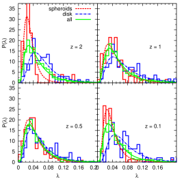
Figure 15.— The $\lambda$-distribution calculated with formula (4) for the different redshifts as indicated in the plots. Green takes all halos into account. The distributions of the spheroids are the red dashed histograms, and those of the disks are blue dot-dashed histograms. The curves are the fits given by equation (7). At all redshifts a split-up of the two different galaxy types is present. The spheroids have their median at the lower $\lambda$-values, while the disks have higher values.

Table 5Calculated Median Values and the Fit Values of the $\lambda$-Distributions

Redshift	All Halos
2	$\lambda_{\mathrm{med}}=0.043$, $\lambda_{0}=0.043$, $\sigma=0.662$
1	$\lambda_{\mathrm{med}}=0.046$, $\lambda_{0}=0.047$, $\sigma=0.635$
0.5	$\lambda_{\mathrm{med}}=0.041$, $\lambda_{0}=0.042$, $\sigma=0.640$
0.1	$\lambda_{\mathrm{med}}=0.042$, $\lambda_{0}=0.043$, $\sigma=0.630$
Redshift	Disks
2	$\lambda_{\mathrm{med}}=0.058$, $\lambda_{0}=0.059$, $\sigma=0.543$
1	$\lambda_{\mathrm{med}}=0.060$, $\lambda_{0}=0.062$, $\sigma=0.644$
0.5	$\lambda_{\mathrm{med}}=0.051$, $\lambda_{0}=0.050$, $\sigma=0.617$
0.1	$\lambda_{\mathrm{med}}=0.069$, $\lambda_{0}=0.064$, $\sigma=0.570$
Redshift	Spheroids
2	$\lambda_{\mathrm{med}}=0.028$, $\lambda_{0}=0.029$, $\sigma=0.497$
1	$\lambda_{\mathrm{med}}=0.042$, $\lambda_{0}=0.042$, $\sigma=0.633$
0.5	$\lambda_{\mathrm{med}}=0.037$, $\lambda_{0}=0.039$, $\sigma=0.620$
0.1	$\lambda_{\mathrm{med}}=0.034$, $\lambda_{0}=0.034$, $\sigma=0.546$

The $\lambda$-distribution for all halos seems to be relatively constant with time, i.e., independent of redshift, which is in agreement with Peirani et al. (2004).

To verify the statistical significance of the differences, we show in Figure 16 the cumulative distributions for the $\lambda$-values, again splitting the halos according to the different galaxy types they host. This illustrates the distances between the two distributions, where the curve for the halos of the spheroidal galaxies is always left of the curve for all halos and the curve of the disk galaxies stays always to the right. The differences are more pronounced for small spins. To quantify the statistical significance of differences in the distributions for the disk and spheroidal galaxies, we apply a Kolmogorov-Smirnov (K-S) test. This test is applied to the two unbinned distributions for the disks and the spheroids. Table 6 shows the calculated values for the maximum distance $D$ and the probability. With the exception of the results at $z=0.5$, this confirms that the spin distributions of the halos hosting disk galaxies are statistically significantly different from the halos hosting spheroidal galaxies.

Table 6K-S Test for the $\lambda$-Distributions

Redshift	$D$	Probability
2	0.563	1.41 $\cdot 10^{-7}$
1	0.319	4.45 $\cdot 10^{-4}$
0.5	0.237	1.45 $\cdot 10^{-2}$
0.1	0.421	6.31 $\cdot 10^{-7}$

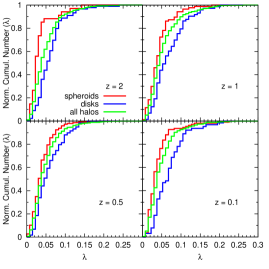
Figure 16.— The $\lambda$-parameter plotted against the normalized cumulative number of halos. Green takes all halos into account, red the spheroidal galaxies, and blue the disk galaxies. The distributions of the disks and the spheroids do not overlap (besides at $z=0.1$ at the higher end). The disks are on the right side, i.e., at higher values, of the distribution for all halos, while the spheroids are on the left, i.e., at lower values.

In this section we have seen that there is a statistical correlation between the morphological type and the overall distribution of the spin parameter $\lambda$. We thus conclude that the total DM halo somehow “knows” about the morphology of the galaxy at its center. At all four considered redshifts the distributions for the spheroids have lower median $\lambda$-values than those of the disks. According to the K-S test, there is a strong indication that they do not originate from the same distribution. On the other hand, we have also found that there are spheroids with even higher $\lambda$-values than disk galaxies.

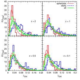
Figure 17.— The $\lambda$-parameter for the DM component within $R_{\mathrm{vir}}$; also in the DM component of all halos (green) there is a broad distribution, which splits into spheroids (red) at lower values, while disks (blue) peak at higher values.

To verify that these differences are intrinsic to the halo and not caused by the contributions of the baryonic component to the spin parameter, we calculated the spin parameter $\lambda_{\mathrm{DM}}$ for the DM component of the halos. Figure 17 shows the $\lambda_{\mathrm{DM}}$-distribution for the baryon run for the four redshifts as indicated in the plots. The green histogram shows $\lambda_{\mathrm{DM}}$ for all halos, the red one stands for the spheroids, and the blue one for disk galaxies. Here again, most prominently visible at redshifts $z=2$ and $z=0.1$, there is a splitting of the two different galaxy types, the distribution of the spheroids peaks at lower values, and that of the disks at higher values. We also perform a K-S test on the two distributions (see Table 7). The values are similar to that of the general $\lambda$-distribution (Table 6).

Table 7K-S Test for the $\lambda_{\mathrm{DM}}$-Distributions

Redshift	$D$	Probability	$D_{\mathrm{DMO}}$	$\mathrm{Probability}_{\mathrm{DMO}}$
2	0.537	5.92 $\cdot 10^{-7}$	0.590	8.14 $\cdot 10^{-8}$
1	0.319	4.45 $\cdot 10^{-4}$	—	—
0.5	0.234	1.65 $\cdot 10^{-2}$	0.285	2.3 $\cdot 10^{-3}$
0.1	0.390	4.60 $\cdot 10^{-6}$	0.370	9.84 $\cdot 10^{-5}$

In the Appendix C we show that this split-up of the galaxy types is also reflected in the spin parameter $\lambda$ of the stellar component.

In order to see whether the differences originate from differences within the DM halo or if they are caused by the interplay between the DM and the baryonic component, we finally compare the run with the baryons to the DM-only control run. We thereto cross-identify the halos of the DM-only run with those of the hydrodynamical run. We search for the corresponding halos in the DM run, allowing the center of the halo to be in a range of 200 kpc around its position in the simulation with baryons, and additionally restrict to halo pairs that only differ by up to 30% in their virial masses. At redshift $z=2$ we found 364 halos in the baryon run that match with the DM-only run, at $z=0.5$ we could assign 609 halos, and at $z=0.1$ we cross-matched 575 halos. We find that the $\lambda_{\mathrm{DM}}$-values of each halo identified in both runs are very similar (see Figure 22 of Appendix ). Since baryons have an effect on the DM, in the two runs the evolution of some of the halos can be quite different, as also discussed in Bett et al. (2010). Therefore, we cannot match every halo.

Figure 18 shows the $\lambda$-distribution for the DM component at three different redshifts. The overall distribution is shown in black. The fit values $\lambda_{0}$ for the DM-only run are slightly lower than for the run with baryons. When we split the halos in the DM-only run according to their galaxy type assigned in the run with baryons, we find a similar split in the distributions as in the run with baryons. At redshift $z=2$ we could use 76 disks and 33 spheroids, at $z=0.5$ there are 55 disks and 143 spheroids, and at $z=0.1$ we cross-matched 53 disks and 99 spheroids. The results of the K-S test (see Table 7) show that these two distributions are unlikely to originate from the same one. It is striking that even in the run without baryons, the split-up of the spin parameter for the different galaxy types is clearly visible. This suggests that the hosting DM halo and, connected with that, the formation history and environment play an important role for the morphology of the resulting galaxy.

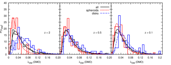
Figure 18.— The $\lambda$-parameter for the DM component for the DM-only run (black) at three redshifts. The red curves show the distribution for halos that were identified in the baryon run and classified as spheroids, while the blue curves show the halos classified as disks in the baryon run. There is a split-up of the galaxy types, which suggests that the morphology could be a result of the formation history.

7. Discussion and Conclusions

We extracted between $400$ and $630$ halos with total halo masses above $5\cdot 10^{11}M_{\odot}$ at four different redshifts from the hydrodynamical, cosmological state-of-the-art simulation Magneticum Pathfinder, which includes detailed treatment of star formation, chemical enrichment, and evolution of supermassive BHs. We investigated the distribution of the spin parameter $\lambda_{k}$ of the different components (DM, stars, hot and cold gas) and the alignment of the angular momentum vectors of those components within the entire halo, as well as within the central 10% of the virial radius. To classify the galaxies according to their morphology, we rotate them such that their angular momentum vector is oriented along the $z$-axis. For this orientation we calculate the circularity parameter $\varepsilon$, which allows a classification based on their circularity distribution. This allows us to define the subset of galaxies clearly identified as spheroidal or disk galaxies and to compare their properties to observations. We additionally performed and analyzed a DM control simulation to test the effect of the baryonic processes and the formation history on the angular momentum within the halos. We summarize our findings as follows:

(i) For all our halos, the stellar component generally has a lower spin than the DM component, while the gas shows a significantly higher spin parameter, especially the cold gas component that dominates the overall spin parameter of the gas. While the distribution of the spin parameters of stars and DM does not show a significant evolution with time, the spin distribution of the gas component significantly evolves toward larger spin values with decreasing redshift.

(ii) In general, the angular momentum vectors of the baryonic components and the DM are well aligned. There is an evolution within these alignments, where at high redshifts the alignment between gas and stars is better than their alignment with the DM component, while at low redshift stars and DM tend to be better aligned.

(iii) When classifying galaxies according to their position within the stellar-mass–specific-angular-momentum plane, we demonstrate that various galaxy properties show smooth transitions, as expected when going from rotation-dominated systems to dispersion-dominated systems. This is most prominently found for the circularity distribution of stars and gas, the cold gas fraction, but also for the spin parameter distribution and the alignments of the angular momenta. Rotation-dominated galaxies have generally larger spin parameters, and the angular momentum vectors of the stars and gas components are aligned. On the contrary, dispersion-dominated galaxies generally have smaller spin parameters and show almost no alignment between the angular momentum vectors of stars and the (however small) gas components.

(iv) Alternatively, when classifying our galaxies according to their circularity distribution in combination with the cold gas content into disk galaxies and spheroidal galaxies, they populate clearly distinguishable regions within the stellar-mass–specific-angular-momentum plane. Using that classification, we lose a significant number of galaxies that cannot be classified within this scheme. Nevertheless, for those galaxies that can be classified the results are in excellent agreement with observations for both spheroidal and disk galaxies.

(v) In disk galaxies the specific angular momentum of the gas is slightly higher than that of the stars, which is in good agreement with recent observations (Obreschkow & Glazebrook, 2014). This is due to the fact that the gas component has contributions from freshly accreted gas with higher specific angular momentum, which will be turned into stars later. This is also reflected in our result that the specific angular momentum of the young stars is slightly larger compared to that of all stars.

(vi) In general, the specific angular momentum of the total halo is higher than the specific angular momentum of the gas in the galaxy. For disk galaxies it accounts for roughly 43% of the value found for the total halo, with no significant redshift evolution.

(vii) Overall, the angular momentum of the total halo is only weakly aligned with the angular momentum of the central part. Here the simulation including baryons shows slightly more alignment than the DM-only simulation. However, we found that in general the halos hosting disk galaxies (in comparison with halos with spheroidal galaxies at their centers) show a better alignment of the angular momentum vectors of the total halo and the central part for the DM component. This is most pronounced at redshift $z\approx 1$, where most disk galaxies are forming.

(viii) The splitting of the galaxies into disk and spheroidal galaxies reveals also a dichotomy in general halo properties: the halos hosting disk galaxies have a slightly larger spin than the halos hosting galaxies classified as spheroidal galaxies. This dichotomy is even reflected in the distribution of the spin parameters in the DM control run, where we cross-identified the halos which in the hydrodynamical simulation host galaxies of different types. This indicates that the formation history of the DM halo plays an important role for defining the morphology of the galaxies.

Our results are based on the classification of galaxies obtained from the circularity of the stellar component ($\varepsilon_{\mathrm{star}}$) in combination with the fraction of cold gas with respect to the stellar mass within the central part of the halo, where the galaxies form. This allows us to select classical disk and spheroidal galaxies, which show very distinct dynamical properties, reflected in their circularity distribution, cold gas fractions, specific angular momentum, and spin and angular momentum vector alignments. They therefore shed light on the main formation mechanism of these galaxies within the cosmological framework.

While our current classification focuses on a selection of galaxies whose properties resemble those of classical spiral and elliptical galaxies, the lion’s share of the galaxies in our simulation cannot be classified as poster child disk or spheroidal galaxies. This again reflects observational facts, since at present day many galaxies exhibit signs of distortions, ongoing merger events, peculiar structures, or other irregularities. For our unclassified galaxies, we clearly see that their properties show a smooth transition between the poster child disks and spheroids, and to understand those transition processes, more complex classification schemes are needed. We suggest that those schemes should consider a differentiation between young and old stellar components, as well as the general distribution of the diverse gas phases in different parts of the galaxies.

Additionally, when comparing to observations, more emphasis needs to be placed on how observational quantities are obtained and how this is mimicked when analyzing simulations. Classifications of galaxy morphologies in cosmological simulations also allow the interpretation of cosmological simulations in various new ways, as already proven in this work, not only for studying the formation and evolution of galaxies but also for studying the relation of AGNs with their host galaxies, as well as for cosmological studies, where the bias of the measurements depends on the morphologies of the galaxies. Therefore, the good agreement of the intrinsic dynamical properties for our classified galaxies with respect to current observations can be seen as a first step to promote cosmological, hydrodynamical simulations for future cosmological studies.

Appendix A Appendix A: Details on the Classification

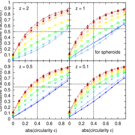
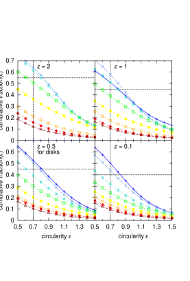
Figure 19.— Left: cumulative fraction of all galaxies in dependency of the circularity $\varepsilon$ of the stars for all four redshifts. The colors reflect the different $b$-value bins, as in Figure 5. From this we estimate the cut for the determination of the spheroidal part of a galaxy. This cut differs for each redshift. Right: cumulative fraction in order to determine the disk part of a galaxy. The values on the $y$-axis are the cumulative values from the corresponding point on the $x$-axis up to an $\varepsilon$-value of 3.

In order to illustrate the choice of the cuts in $\varepsilon_{\mathrm{star}}$ used for the classification of our galaxies, we show the cumulative circularity distribution for spheroids (left panels) and the ‘anti-’cumulative distribution for disk galaxies (right panels) in Figure 19. For the spheroids we sum up the fractions from $-\varepsilon$ to $\varepsilon$ of the distributions shown in Figure 5, $f(x)=\sum_{-x}^{x}fraction(\varepsilon)$. The cut is drawn between the halos of the $b$-value-bin that show a clear behavior of spheroids at the corresponding redshift. The same is done for the disk galaxies, besides that here we sum up the fraction from $\varepsilon$ to $3$, $f(x)=\sum_{x}^{3}fraction(\varepsilon)$.

         

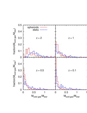
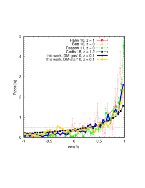
Figure 20.— Left: fraction of the mass of the cold gas with respect to the stellar mass, both within the inner 10% of the virial radius. The cold gas fraction decreases continuously with decreasing redshift, for spheroids faster than for disk galaxies. Note that at $z=2$ most spheroidal galaxies have a mass fraction larger than 10%. At $z=0.1$ the disk galaxies are divided into two populations, one with a fraction higher than 30% and the other having less than 10%. We suggest that the second population comprises lenticular galaxies. Right: probability distribution function of the alignment of the galaxies compared to their DM halo in comparison with previous studies, as indicated in the plot.

In the left panels of Figure 20 we show that at high redshift there are many spheroidal galaxies (red histograms, classified with $\varepsilon_{\mathrm{star}}$) with a high fraction of cold gas mass with respect to the stars. This fraction decreases very fast with decreasing redshift. Disk galaxies (blue) have a higher amount of cold gas at all times, especially at high redshift. Still, at low redshift there are many disk galaxies that have less than 10% cold gas. Those galaxies actually resemble S0 properties and are not classical “disks.”

Table 8Upper/Lower Limits for the Classification Criteria

Redshift	$\varepsilon_{\mathrm{star}}$, $d$	$\varepsilon_{\mathrm{star}}$, $s$	$M_{\mathrm{cold}}/M_{\mathrm{star}}$, $d$	$M_{\mathrm{cold}}/M_{\mathrm{star}}$, $s$
2	0.55	0.5	0.5	0.35
1	0.45	0.55	0.35	0.2
0.5	0.45	0.55	0.275	0.125
0.1	0.4	0.6	0.215	0.065

In Table 8 we list the values of the cuts for the classification criteria. The values for the spheroids should be understood as an upper limit, while for the disks they represent a lower limit.

Appendix B Appendix B: The Alignment of the Galaxy with Its DM Halo

The right panel of Figure 20 shows the probability distribution function of the cosine of the angles between the innermost 10% of the virial radius of our disk galaxies and the hosting DM halo. The solid blue line stands for the gaseous component, and the yellow dashed line for the stellar component. We extracted the other data points from Codis et al. (2015) for an easier comparison with previous works. Overall, our results are in good agreement with previous studies. We find that our disk galaxies have a slightly weaker alignment than those of Bett et al. (2010) and Deason et al. (2011). Our results agree well with Hahn et al. (2010). Codis et al. (2015) report slightly less aligned galaxies.

Appendix C Appendix C: The Spin Parameter $\lambda$

The left panels of Figure 21 show the $\lambda$-parameter of the stellar component within the innermost 10% of the virial radius against that of the total DM halo for individual halos classified as spheroids (red circles) and disks (blue diamonds). We can clearly see the split-up of the two populations, where disk galaxies have a higher stellar spin than the spheroids.

On the right side of Figure 21 we show the $\lambda$-distribution for the stellar component within the total virial radius. We also see a split-up of the spheroidal (red) and disk (blue) galaxies. The stars in disk galaxies have a higher spin than in spheroids. This seems plausible, since most stars in disk galaxies are found in the disk while most stars in spheroidal galaxies are found in the dominant bulge and thus are more spherically distributed. Hence, they have a net spin that is lower than that in disk galaxies, where the stars sum up their spin. This also shows that the stars trace the formation history of the galaxies. The stars in disks form out of the fresh gas with high angular momentum, while in spheroids many stars are accreted (via minor/major mergers).

         

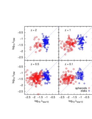
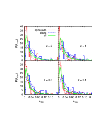
Figure 21.— Left: $\lambda$-parameter for the stellar component in the innermost 10% against that of the DM of the entire DM halo, at four different redshifts, divided into spheroidal (red circles) and disk (blue diamonds) galaxies. Right: $\lambda$-distribution for the stellar component at four different redshifts, divided into spheroidal (red dashed) and disk (blue dot-dashed) galaxies. The stellar component of spheroids has a very low median value, whereas the disk galaxies have a higher one at all shown redshifts.

Table 9K-S Test for the $\lambda_{\mathrm{star}}$-Distributions

Redshift	$D$	Probability
2	0.558	1.81 $\cdot 10^{-7}$
1	0.364	3.42 $\cdot 10^{-5}$
0.5	0.443	6.62 $\cdot 10^{-8}$
0.1	0.493	2.40 $\cdot 10^{-9}$

In Table 9 we show the results from the K-S test for the $\lambda_{\mathrm{star}}$-distribution. The two distributions for the disk and the spheroidal galaxies do not originate from the same distribution.

In order to see how the $\lambda$-parameter behaves for individual halos in the baryon and the DM-only runs, we identified the same halos in the baryonic and the DM-only run (as described earlier). The left panels of the left figure of Figure 22 show the $\lambda$-parameter of the DM component against the $\lambda$-parameter of the DM-only run in logarithmic scaling for spheroids at redshifts $z=2$ (upper panel) and $z=0.1$ (lower panel). The values of the $\lambda$-parameter of the corresponding halos in both runs are similar. The stellar mass within 10% of the virial radius of the baryon run is color-coded. On the right panels we find the $\lambda_{\mathrm{DM}}$-values for the disks. At redshift $z=2$ (upper panel) we note a slight tendency for the $\lambda_{\mathrm{DM}}$ to decrease with increasing stellar mass. The less massive disks tend to have higher $\lambda$-values. This is in agreement with Berta et al. (2008), who computed the DM spin parameter of $\approx$52,000 disk galaxies from the SDSS (for details of the sample see references in Berta et al. (2008)). They found a clear anticorrelation between the DM spin and the stellar mass, i.e., that galaxies with a low mass in general have higher DM spins. For the spheroidal galaxies we do not see this trend. In addition, this figure demonstrates that a high $\lambda$ does not automatically lead to a disk galaxy and a small $\lambda$ is no guarantee for a spheroidal galaxy. The scatter is equal for both galaxy types. The fact that $\lambda_{\mathrm{DM}}$ in the whole virial radius is similar in the DM-only and the baryon run is in good agreement with Bryan et al. (2013).

Appendix D Appendix D: The Radial Specific Angular Momentum Profiles

         

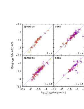
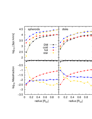
Figure 22.— Left: $\lambda$-parameter plotted logarithmically for the DM component, on the $x$-axis the $\lambda$ for the baryon run and on the $y$-axis for the DM-only run; the color codes the stellar mass within the inner 10% of the virial radius. On the left panels are the spheroids and on the right panels the disks. The upper panels show redshift $z=2$ and the lower ones $z=0.1$. Right: specific angular momentum (top panels) and the mass fractions (bottom panels) against distance from the center for the cold gas (blue), hot gas (red), stars (yellow), and DM (black) of our sample of galaxies at $z=0.1$. On each left-hand side we show the analysis for the spheroidal galaxies, and on each right-hand side that for the disks.

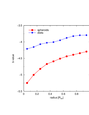
Figure 23.— The radial profile of the $b$-value averaged over spheroids (red circles) and disks (blue diamonds).

In order to illustrate the behavior of the specific angular momentum of the different components, we show on the right-hand side of Figure 22 the mean of our sample of spheroidal (left panel) and disk galaxies (right panel) at $z=0.1$. In the upper panels we plot the differential specific angular momenta of the different components against radius, and in the lower panels we plot the individual mass fractions of the corresponding components against radius. The $x$-axis is linearly binned with a bin size of 10% of the virial radius of a halo. The specific angular momentum of the two galaxy types increases from the center of the halo up to the virial radius. On the outer parts the specific angular momentum of the hot gas follows the DM, while the specific angular momentum of the stars follows that of the cold gas. This might be due to the infalling substructures, which mostly consist of small gas clumps with stars that formed out of it. The main difference of the two galaxy types becomes clear in the center: the angular momentum of the stars drops dramatically in spheroidal galaxies, while in disk galaxies it remains higher than that of the DM. With respect to the baryons, the outer region is dominated by the hot gas, which behaves similarly for spheroids and disks.

Figure 23 shows the radial profile of the $b$-value. Therefore, we calculated

$$b=\mathrm{log}_{10}\left(\frac{j_{\mathrm{star}}(\leq r)}{\mathrm{kpc}~{}\mathrm{km/s}}\right)-\frac{2}{3}\mathrm{log}_{10}\left(\frac{M_{\mathrm{star}}(\leq r)}{M_{\odot}}\right),$$ (D1)

averaged over the spheroids and disks. The slope is steeper for the spheroids than for the disk galaxies. This illustrates that the measurement of the kinematic properties is more sensitive to the radius for spheroidal than for disk galaxies.

References

- Abadi et al. (2003) Abadi, M. G., Navarro, J. F., Steinmetz, M., & Eke, V. R. 2003, ApJ, 597, 21
- Arth et al. (2014) Arth, A., Dolag, K., Beck, A. M., Petkova, M., & Lesch, H. 2014, ArXiv:1412.6533
- Aubert et al. (2004) Aubert, D., Pichon, C., & Colombi, S. 2004, MNRAS, 352, 376
- Bailin & Steinmetz (2005) Bailin, J. & Steinmetz, M. 2005, ApJ, 627, 647
- Barnes & Efstathiou (1987) Barnes, J. & Efstathiou, G. 1987, ApJ, 319, 575
- Barnes & Hernquist (1996) Barnes, J. E. & Hernquist, L. 1996, ApJ, 471, 115
- Beck et al. (2015) Beck, A. M., Murante, G., Arth, A., Remus, R.-S., Teklu, A. F., Donnert, J. M. F., Planelles, S., Beck, M. C., Foerster, P., Imgrund, M., Dolag, K., & Borgani, S. 2015, ArXiv:1502.07358
- Berta et al. (2008) Berta, Z. K., Jimenez, R., Heavens, A. F., & Panter, B. 2008, MNRAS, 391, 197
- Bett et al. (2010) Bett, P., Eke, V., Frenk, C. S., Jenkins, A., & Okamoto, T. 2010, MNRAS, 404, 1137
- Biffi & Maio (2013) Biffi, V. & Maio, U. 2013, MNRAS, 436, 1621
- Bondi (1952) Bondi, H. 1952, MNRAS, 112, 195
- Bondi & Hoyle (1944) Bondi, H. & Hoyle, F. 1944, MNRAS, 104, 273
- Brook et al. (2004) Brook, C. B., Kawata, D., Gibson, B. K., & Flynn, C. 2004, MNRAS, 349, 52
- Bryan et al. (2013) Bryan, S. E., Kay, S. T., Duffy, A. R., Schaye, J., Dalla Vecchia, C., & Booth, C. M. 2013, MNRAS, 429, 3316
- Bullock et al. (2001) Bullock, J. S., Dekel, A., Kolatt, T. S., Kravtsov, A. V., Klypin, A. A., Porciani, C., & Primack, J. R. 2001, ApJ, 555, 240
- Cappellari et al. (2011) Cappellari, M., Emsellem, E., Krajnović, D., McDermid, R. M., Scott, N., Verdoes Kleijn, G. A., Young, L. M., Alatalo, K., Bacon, R., Blitz, L., Bois, M., Bournaud, F., Bureau, M., Davies, R. L., Davis, T. A., de Zeeuw, P. T., Duc, P.-A., Khochfar, S., Kuntschner, H., Lablanche, P.-Y., Morganti, R., Naab, T., Oosterloo, T., Sarzi, M., Serra, P., & Weijmans, A.-M. 2011, MNRAS, 413, 813
- Chabrier (2003) Chabrier, G. 2003, PASP, 115, 763
- Chen et al. (2003) Chen, D. N., Jing, Y. P., & Yoshikaw, K. 2003, ApJ, 597, 35
- Codis et al. (2015) Codis, S., Gavazzi, R., Dubois, Y., Pichon, C., Benabed, K., Desjacques, V., Pogosyan, D., Devriendt, J., & Slyz, A. 2015, MNRAS, 448, 3391
- Croft et al. (2009) Croft, R. A. C., Di Matteo, T., Springel, V., & Hernquist, L. 2009, MNRAS, 400, 43
- Danovich et al. (2015) Danovich, M., Dekel, A., Hahn, O., Ceverino, D., & Primack, J. 2015, MNRAS, 449, 2087
- Davis et al. (1985) Davis, M., Efstathiou, G., Frenk, C. S., & White, S. D. M. 1985, ApJ, 292, 371
- Davis et al. (2011) Davis, T. A., Alatalo, K., Sarzi, M., Bureau, M., Young, L. M., Blitz, L., Serra, P., Crocker, A. F., Krajnović, D., McDermid, R. M., Bois, M., Bournaud, F., Cappellari, M., Davies, R. L., Duc, P.-A., de Zeeuw, P. T., Emsellem, E., Khochfar, S., Kuntschner, H., Lablanche, P.-Y., Morganti, R., Naab, T., Oosterloo, T., Scott, N., & Weijmans, A.-M. 2011, MNRAS, 417, 882
- Deason et al. (2011) Deason, A. J., McCarthy, I. G., Font, A. S., Evans, N. W., Frenk, C. S., Belokurov, V., Libeskind, N. I., Crain, R. A., & Theuns, T. 2011, MNRAS, 415, 2607
- Di Matteo et al. (2005) Di Matteo, T., Springel, V., & Hernquist, L. 2005, Nature, 433, 604
- Dolag et al. (2009) Dolag, K., Borgani, S., Murante, G., & Springel, V. 2009, MNRAS, 399, 497
- Dolag et al. (2004) Dolag, K., Jubelgas, M., Springel, V., Borgani, S., & Rasia, E. 2004, ApJ, 606, L97
- Dolag et al. (2005) Dolag, K., Vazza, F., Brunetti, G., & Tormen, G. 2005, MNRAS, 364, 753
- Donnert et al. (2013) Donnert, J., Dolag, K., Brunetti, G., & Cassano, R. 2013, MNRAS, 429, 3564
- Doroshkevich (1970) Doroshkevich, A. G. 1970, Astrofizika, 6, 581
- Dubois et al. (2014) Dubois, Y., Pichon, C., Welker, C., Le Borgne, D., Devriendt, J., Laigle, C., Codis, S., Pogosyan, D., Arnouts, S., Benabed, K., Bertin, E., Blaizot, J., Bouchet, F., Cardoso, J.-F., Colombi, S., de Lapparent, V., Desjacques, V., Gavazzi, R., Kassin, S., Kimm, T., McCracken, H., Milliard, B., Peirani, S., Prunet, S., Rouberol, S., Silk, J., Slyz, A., Sousbie, T., Teyssier, R., Tresse, L., Treyer, M., Vibert, D., & Volonteri, M. 2014, MNRAS, 444, 1453
- Eke et al. (1996) Eke, V. R., Cole, S., & Frenk, C. S. 1996, MNRAS, 282, 263
- Fabjan et al. (2010) Fabjan, D., Borgani, S., Tornatore, L., Saro, A., Murante, G., & Dolag, K. 2010, MNRAS, 401, 1670
- Fall (1983) Fall, S. M. 1983, in IAU Symposium, Vol. 100, Internal Kinematics and Dynamics of Galaxies, ed. E. Athanassoula, 391–398
- Fall & Efstathiou (1980) Fall, S. M. & Efstathiou, G. 1980, MNRAS, 193, 189
- Fall & Romanowsky (2013) Fall, S. M. & Romanowsky, A. J. 2013, ApJ, 769, L26
- Ferland et al. (1998) Ferland, G. J., Korista, K. T., Verner, D. A., Ferguson, J. W., Kingdon, J. B., & Verner, E. M. 1998, PASP, 110, 761
- Genel et al. (2015) Genel, S., Fall, S. M., Hernquist, L., Vogelsberger, M., Snyder, G. F., Rodriguez-Gomez, V., Sijacki, D., & Springel, V. 2015, ApJ, 804, L40
- González-García et al. (2009) González-García, A. C., Oñorbe, J., Domínguez-Tenreiro, R., & Gómez-Flechoso, M. Á. 2009, A&A, 497, 35
- Governato et al. (2007) Governato, F., Willman, B., Mayer, L., Brooks, A., Stinson, G., Valenzuela, O., Wadsley, J., & Quinn, T. 2007, MNRAS, 374, 1479
- Haardt & Madau (2001) Haardt, F. & Madau, P. 2001, in Clusters of Galaxies and the High Redshift Universe Observed in X-rays, ed. D. M. Neumann & J. T. V. Tran
- Hahn et al. (2010) Hahn, O., Teyssier, R., & Carollo, C. M. 2010, MNRAS, 405, 274
- Hernandez & Cervantes-Sodi (2006) Hernandez, X. & Cervantes-Sodi, B. 2006, MNRAS, 368, 351
- Hernandez et al. (2007) Hernandez, X., Park, C., Cervantes-Sodi, B., & Choi, Y.-Y. 2007, MNRAS, 375, 163
- Hirschmann et al. (2014) Hirschmann, M., Dolag, K., Saro, A., Bachmann, L., Borgani, S., & Burkert, A. 2014, MNRAS, 442, 2304
- Hoyle & Lyttleton (1939) Hoyle, F. & Lyttleton, R. A. 1939, Proceedings of the Cambridge Philosophical Society, 35, 405
- Johansson et al. (2012) Johansson, P. H., Naab, T., & Ostriker, J. P. 2012, ApJ, 754, 115
- Khandai et al. (2015) Khandai, N., Di Matteo, T., Croft, R., Wilkins, S., Feng, Y., Tucker, E., DeGraf, C., & Liu, M.-S. 2015, MNRAS, 450, 1349
- Kimm et al. (2011) Kimm, T., Devriendt, J., Slyz, A., Pichon, C., Kassin, S. A., & Dubois, Y. 2011, ArXiv:1106.0538
- Komatsu et al. (2011) Komatsu, E., Smith, K. M., Dunkley, J., Bennett, C. L., Gold, B., Hinshaw, G., Jarosik, N., Larson, D., Nolta, M. R., Page, L., Spergel, D. N., Halpern, M., Hill, R. S., Kogut, A., Limon, M., Meyer, S. S., Odegard, N., Tucker, G. S., Weiland, J. L., Wollack, E., & Wright, E. L. 2011, ApJS, 192, 18
- Lees et al. (1991) Lees, J. F., Knapp, G. R., Rupen, M. P., & Phillips, T. G. 1991, ApJ, 379, 177
- Leroy et al. (2008) Leroy, A. K., Walter, F., Brinks, E., Bigiel, F., de Blok, W. J. G., Madore, B., & Thornley, M. D. 2008, AJ, 136, 2782
- Macciò et al. (2008) Macciò, A. V., Dutton, A. A., & van den Bosch, F. C. 2008, MNRAS, 391, 1940
- McDonald et al. (2014) McDonald, M., Benson, B. A., Vikhlinin, A., Aird, K. A., Allen, S. W., Bautz, M., Bayliss, M., Bleem, L. E., & et al. 2014, ApJ, 794, 67
- Meza et al. (2003) Meza, A., Navarro, J. F., Steinmetz, M., & Eke, V. R. 2003, ApJ, 590, 619
- Mo et al. (1998) Mo, H. J., Mao, S., & White, S. D. M. 1998, MNRAS, 295, 319
- Murante et al. (2015) Murante, G., Monaco, P., Borgani, S., Tornatore, L., Dolag, K., & Goz, D. 2015, MNRAS, 447, 178
- Naab et al. (2006) Naab, T., Jesseit, R., & Burkert, A. 2006, MNRAS, 372, 839
- Naab et al. (2009) Naab, T., Johansson, P. H., & Ostriker, J. P. 2009, ApJ, 699, L178
- Navarro & Benz (1991) Navarro, J. F. & Benz, W. 1991, ApJ, 380, 320
- Navarro & Steinmetz (1997) Navarro, J. F. & Steinmetz, M. 1997, ApJ, 478, 13
- Navarro & White (1994) Navarro, J. F. & White, S. D. M. 1994, MNRAS, 267, 401
- Obreschkow & Glazebrook (2014) Obreschkow, D. & Glazebrook, K. 2014, ApJ, 784, 26
- Okamoto et al. (2005) Okamoto, T., Eke, V. R., Frenk, C. S., & Jenkins, A. 2005, MNRAS, 363, 1299
- Oser et al. (2010) Oser, L., Ostriker, J. P., Naab, T., Johansson, P. H., & Burkert, A. 2010, ApJ, 725, 2312
- Padovani & Matteucci (1993) Padovani, P. & Matteucci, F. 1993, ApJ, 416, 26
- Peebles (1969) Peebles, P. J. E. 1969, ApJ, 155, 393
- Peebles (1971) —. 1971, A&A, 11, 377
- Peebles (1993) Peebles, P. J. E. 1993, Principles of Physical Cosmology, 1st edn. (Princeton University Press)
- Peirani et al. (2004) Peirani, S., Mohayaee, R., & de Freitas Pacheco, J. A. 2004, MNRAS, 348, 921
- Pichon et al. (2011) Pichon, C., Pogosyan, D., Kimm, T., Slyz, A., Devriendt, J., & Dubois, Y. 2011, MNRAS, 418, 2493
- Planck Collaboration et al. (2013) Planck Collaboration, Ade, P. A. R., Aghanim, N., Arnaud, M., Ashdown, M., Atrio-Barandela, F., Aumont, J., Baccigalupi, C., Balbi, A., Banday, A. J., & et al. 2013, A&A, 550, A131
- Remus et al. (2013) Remus, R.-S., Burkert, A., Dolag, K., Johansson, P. H., Naab, T., Oser, L., & Thomas, J. 2013, ApJ, 766, 71
- Remus et al. (2015) Remus, R.-S., Dolag, K., Bachmann, L. K., Beck, A. M., Burkert, A., Hirschmann, M., & Teklu, A. 2015, in IAU Symposium, Vol. 309, IAU Symposium, ed. B. L. Ziegler, F. Combes, H. Dannerbauer, & M. Verdugo, 145–148
- Romanowsky & Fall (2012) Romanowsky, A. J. & Fall, S. M. 2012, ApJS, 203, 17
- Sales et al. (2012) Sales, L. V., Navarro, J. F., Theuns, T., Schaye, J., White, S. D. M., Frenk, C. S., Crain, R. A., & Dalla Vecchia, C. 2012, MNRAS, 423, 1544
- Salim & Rich (2010) Salim, S. & Rich, R. M. 2010, ApJ, 714, L290
- Scannapieco et al. (2008) Scannapieco, C., Tissera, P. B., White, S. D. M., & Springel, V. 2008, MNRAS, 389, 1137
- Scannapieco et al. (2012) Scannapieco, C., Wadepuhl, M., Parry, O. H., Navarro, J. F., Jenkins, A., Springel, V., Teyssier, R., Carlson, E., Couchman, H. M. P., Crain, R. A., Dalla Vecchia, C., Frenk, C. S., Kobayashi, C., Monaco, P., Murante, G., Okamoto, T., Quinn, T., Schaye, J., Stinson, G. S., Theuns, T., Wadsley, J., White, S. D. M., & Woods, R. 2012, MNRAS, 423, 1726
- Scannapieco et al. (2009) Scannapieco, C., White, S. D. M., Springel, V., & Tissera, P. B. 2009, MNRAS, 396, 696
- Schaye et al. (2015) Schaye, J., Crain, R. A., Bower, R. G., Furlong, M., Schaller, M., Theuns, T., Dalla Vecchia, C., Frenk, C. S., McCarthy, I. G., Helly, J. C., Jenkins, A., Rosas-Guevara, Y. M., White, S. D. M., Baes, M., Booth, C. M., Camps, P., Navarro, J. F., Qu, Y., Rahmati, A., Sawala, T., Thomas, P. A., & Trayford, J. 2015, MNRAS, 446, 521
- Schaye et al. (2010) Schaye, J., Dalla Vecchia, C., Booth, C. M., Wiersma, R. P. C., Theuns, T., Haas, M. R., Bertone, S., Duffy, A. R., McCarthy, I. G., & van de Voort, F. 2010, MNRAS, 402, 1536
- Schlachtberger, D.P. (2014) Schlachtberger, D.P. 2014, Master’s thesis, Ludwig-Maximilians-Universität München
- Shakura & Sunyaev (1973) Shakura, N. I. & Sunyaev, R. A. 1973, A&A, 24, 337
- Sharma & Steinmetz (2005) Sharma, S. & Steinmetz, M. 2005, ApJ, 628, 21
- Sharma et al. (2012) Sharma, S., Steinmetz, M., & Bland-Hawthorn, J. 2012, ApJ, 750, 107
- Shen et al. (2003) Shen, S., Mo, H. J., White, S. D. M., Blanton, M. R., Kauffmann, G., Voges, W., Brinkmann, J., & Csabai, I. 2003, MNRAS, 343, 978
- Sijacki et al. (2007) Sijacki, D., Springel, V., Di Matteo, T., & Hernquist, L. 2007, MNRAS, 380, 877
- Sijacki et al. (2012) Sijacki, D., Vogelsberger, M., Kereš, D., Springel, V., & Hernquist, L. 2012, MNRAS, 424, 2999
- Spitzer (1962) Spitzer, L. 1962, Physics of Fully Ionized Gases
- Springel (2005) Springel, V. 2005, MNRAS, 364, 1105
- Springel et al. (2005) Springel, V., Di Matteo, T., & Hernquist, L. 2005, MNRAS, 361, 776
- Springel & Hernquist (2003) Springel, V. & Hernquist, L. 2003, MNRAS, 339, 289
- Springel & Hernquist (2005) —. 2005, ApJ, 622, L9
- Springel et al. (2001a) Springel, V., White, S. D. M., Tormen, G., & Kauffmann, G. 2001a, MNRAS, 328, 726
- Springel et al. (2001b) Springel, V., Yoshida, N., & White, S. D. M. 2001b, Nature, 6, 79
- Steinborn et al. (2015) Steinborn, L. K., Dolag, K., Hirschmann, M., Prieto, M. A., & Remus, R.-S. 2015, MNRAS, 448, 1504
- Stewart et al. (2013) Stewart, K. R., Brooks, A. M., Bullock, J. S., Maller, A. H., Diemand, J., Wadsley, J., & Moustakas, L. A. 2013, ApJ, 769, 74
- Stewart et al. (2011) Stewart, K. R., Kaufmann, T., Bullock, J. S., Barton, E. J., Maller, A. H., Diemand, J., & Wadsley, J. 2011, ApJ, 738, 39
- Teklu et al. (2015) Teklu, A., Remus, R.-S., Dolag, K., & Burkert, A. 2015, in IAU Symposium, Vol. 309, IAU Symposium, ed. B. L. Ziegler, F. Combes, H. Dannerbauer, & M. Verdugo, 349–349
- Thielemann et al. (2003) Thielemann, F.-K., Argast, D., Brachwitz, F., Hix, W. R., Höflich, P., Liebendörfer, M., Martinez-Pinedo, G., Mezzacappa, A., Panov, I., & Rauscher, T. 2003, Nuclear Physics A, 718, 139
- Toomre (1977) Toomre, A. 1977, in Evolution of Galaxies and Stellar Populations, ed. B. M. Tinsley & R. B. G. Larson, D. Campbell, 401
- Tornatore et al. (2007) Tornatore, L., Borgani, S., Dolag, K., & Matteucci, F. 2007, MNRAS, 382, 1050
- Torrey et al. (2015) Torrey, P., Snyder, G. F., Vogelsberger, M., Hayward, C. C., Genel, S., Sijacki, D., Springel, V., Hernquist, L., Nelson, D., Kriek, M., Pillepich, A., Sales, L. V., & McBride, C. K. 2015, MNRAS, 447, 2753
- Trowland et al. (2013) Trowland, H. E., Lewis, G. F., & Bland-Hawthorn, J. 2013, ApJ, 762, 72
- Übler et al. (2014) Übler, H., Naab, T., Oser, L., Aumer, M., Sales, L. V., & White, S. D. M. 2014, MNRAS, 443, 2092
- van den Bosch et al. (2002) van den Bosch, F. C., Abel, T., Croft, R. A. C., Hernquist, L., & White, S. D. M. 2002, ApJ, 576, 21
- van den Hoek & Groenewegen (1997) van den Hoek, L. B. & Groenewegen, M. A. T. 1997, A&AS, 123, 305
- Vogelsberger et al. (2014) Vogelsberger, M., Genel, S., Springel, V., Torrey, P., Sijacki, D., Xu, D., Snyder, G., Nelson, D., & Hernquist, L. 2014, MNRAS, 444, 1518
- Walter et al. (2008) Walter, F., Brinks, E., de Blok, W. J. G., Bigiel, F., Kennicutt, Jr., R. C., Thornley, M. D., & Leroy, A. 2008, AJ, 136, 2563
- Welker et al. (2014) Welker, C., Devriendt, J., Dubois, Y., Pichon, C., & Peirani, S. 2014, MNRAS, 445, L46
- White (1978) White, S. D. M. 1978, MNRAS, 184, 185
- White (1979) —. 1979, ApJ, 229, L9
- White & Rees (1978) White, S. D. M. & Rees, M. J. 1978, MNRAS, 183, 341
- Wiersma et al. (2009) Wiersma, R. P. C., Schaye, J., & Smith, B. D. 2009, MNRAS, 393, 99
- Woosley & Weaver (1995) Woosley, S. E. & Weaver, T. A. 1995, ApJS, 101, 181
- Young et al. (2011) Young, L. M., Bureau, M., Davis, T. A., Combes, F., McDermid, R. M., Alatalo, K., Blitz, L., Bois, M., Bournaud, F., Cappellari, M., Davies, R. L., de Zeeuw, P. T., Emsellem, E., Khochfar, S., Krajnović, D., Kuntschner, H., Lablanche, P.-Y., Morganti, R., Naab, T., Oosterloo, T., Sarzi, M., Scott, N., Serra, P., & Weijmans, A.-M. 2011, MNRAS, 414, 940
- Young et al. (2014) Young, L. M., Scott, N., Serra, P., Alatalo, K., Bayet, E., Blitz, L., Bois, M., Bournaud, F., Bureau, M., Crocker, A. F., Cappellari, M., Davies, R. L., Davis, T. A., de Zeeuw, P. T., Duc, P.-A., Emsellem, E., Khochfar, S., Krajnović, D., Kuntschner, H., McDermid, R. M., Morganti, R., Naab, T., Oosterloo, T., Sarzi, M., & Weijmans, A.-M. 2014, MNRAS, 444, 3408
- Zavala et al. (2008) Zavala, J., Okamoto, T., & Frenk, C. S. 2008, MNRAS, 387, 364