The angle-averaged squeezed limit of nonlinear matter $\bm{N}$-point functions

Abstract

We show that in a certain, angle-averaged squeezed limit, the $N$-point function of matter is related to the response of the matter power spectrum to a long-wavelength density perturbation, $P^{-1}d^{n}P(k|\delta_{L})/d\delta_{L}^{n}|_{\delta_{L}=0}$, with $n=N-2$. By performing N-body simulations with a homogeneous overdensity superimposed on a flat Friedmann-Robertson-Lemaître-Walker (FRLW) universe using the separate universe approach, we obtain measurements of the nonlinear matter power spectrum response up to $n=3$, which is equivalent to measuring the fully nonlinear matter $3-$ to $5-$point function in this squeezed limit. The sub-percent to few percent accuracy of those measurements is unprecedented. We then test the hypothesis that nonlinear $N$-point functions at a given time are a function of the linear power spectrum at that time, which is predicted by standard perturbation theory (SPT) and its variants that are based on the ideal pressureless fluid equations. Specifically, we compare the responses computed from the separate universe simulations and simulations with a rescaled initial (linear) power spectrum amplitude. We find discrepancies of 10% at $k\simeq 0.2-0.5\,h\,{\rm Mpc}^{-1}$ for $5-$ to $3-$point functions at $z=0$. The discrepancy occurs at higher wavenumbers at $z=2$. Thus, SPT and its variants, carried out to arbitrarily high order, are guaranteed to fail to describe matter $N$-point functions ($N>2$) around that scale.

1 Introduction

Mode-coupling plays a fundamental role in cosmology. Long and short wavelength modes are coupled by nonlinear gravitational evolution of matter density fluctuations and the formation of dark matter halos and galaxies, as well as via the physics of inflation, i.e., primordial non-Gaussianity. The traditional way of characterizing the mode coupling is to study $N$-point correlation functions of matter, halo, and galaxy density fields, as well as of fluctuations of the cosmic microwave background, where the mode coupling enters at $N>2$. The $N$-point functions of matter density fields in particular contain a rich amount of information on gravity and the expansion history of the Universe. At $N>2$, gravity produces specific non-Gaussian signatures that can be used to test the physics of structure formation in the Universe, and must be accounted for when attempting to connect large-scale structure with the statistics of the initial conditions in order to search for primordial non-Gaussianity.

A major challenge is that, beyond the power spectrum, the calculation of (connected) nonlinear $N$-point functions becomes increasingly difficult. Consider the gold standard for predicting the statistics of matter density, N-body simulations. First, a large number of modes is necessary to measure the correlation functions with sufficient precision since the cosmic variance noise is significant. This demands large computational resources. Second, higher $N$-point functions are more sensitive to transients [1, 2] from the finite starting redshift and to mass resolution effects. Third, estimators for higher $N$-point functions become more computationally intensive and difficult to handle. On the theoretical side, the predictions for the bispectrum and higher $N$-point functions likewise become more cumbersome, with terms at any given order in perturbation theory rapidly proliferating with $N$. An analogous effect happens in the halo model, with 1- to $N$-halo terms having to be calculated for the $N$-point function.

Figure 1: Sketch of the squeezed limit configuration of matter $N$-point functions considered in this paper. $\mathbf{k}_{1},\cdots,\mathbf{k}_{n}$ denote the long-wavelength modes which are spherically averaged in Eq. (1.1), while $\mathbf{k},\,\mathbf{k}^{\prime}$ denote the small-scale modes which are allowed to be fully nonlinear.

This provides the motivation to study a certain limit considered in this paper where the nonlinear $N$-point functions become simpler and physically more transparent. The limit we consider is a specific case of the so-called “squeezed limit”, where there is a hierarchy between two large wavenumbers $\mathbf{k},\,\mathbf{k}^{\prime}$ and $N-2$ small wavenumbers $\mathbf{k}_{1},\cdots\mathbf{k}_{n}$. The configuration corresponding to this limit is illustrated in figure 1.

The squeezed limit of dark matter $N$-point functions has recently been the subject of a large body of work in the context of the so-called “consistency relations” [3, 4, 5, 6, 7, 8, 9, 10, 11, 12, 13, 14, 15]. The contributions to $N$-point functions in the squeezed limit are ordered by the ratio of wavenumbers $k_{i}/k$, which is assumed to be much less than one. The lowest order contributions, up $\propto(k_{i}/k)^{-1}$ when the $N$-point function is written in terms of the overdensity $\delta$, are fixed by the requirement that a uniform potential perturbation as well as a uniform velocity (boost) do not lead to any locally observable effect on the density field, as demanded by the equivalence principle [3, 4, 9, 16]. They are also referred to as “kinematical contributions”. Here we focus on the next order contribution, $\propto(k_{i}/k)^{0}$, which is the lowest order at which a physical coupling of long- and short-wavelength modes happens. More precisely, the contributions at this order correspond to the impact of a uniform long-wavelength density or tidal perturbation. When considering equal-time $N$-point functions, which we do throughout, and subhorizon perturbations $k_{i}\gg aH$, the kinematical contributions disappear, and the physical $(k_{i}/k)^{0}$ contributions are the leading contribution to the $N$-point function in the squeezed limit.

In this paper, we disregard tidal fields, which leads us to first angle-average over the $N-2$ small momenta (wavenumbers) in the $N$-point function. Specifically, we consider $\mathcal{S}_{N-2}$ defined through

$$\mathcal{S}_{N-2}(k,k^{\prime};k_{1},\cdots,k_{N-2})\equiv\> \int\frac{d^{2}\hat{\mathbf{k}}_{1}}{4\pi}\cdots\int\frac{d^{2}\hat{\mathbf{k}}_{N-2}}{4\pi}\left\langle\delta(\mathbf{k})\delta(\mathbf{k}^{\prime})\delta(\mathbf{k}_{1})\cdots\delta(\mathbf{k}_{N-2})\right\rangle^{\prime}_{c}\,,$$ (1.1)

where $\hat{\mathbf{k}}_{i}$ are unit vectors and $\left\langle\delta(\mathbf{k}_{1})\cdots\delta(\mathbf{k}_{N})\right\rangle^{\prime}_{c}$ denotes the nonlinear connected matter $N$-point function with the momentum constraint $(2\pi)^{3}\delta_{D}(\mathbf{k}_{1}+\cdots+\mathbf{k}_{N})$ dropped. Note that the momentum constraint fixes $\mathbf{k}^{\prime}$ in terms of $\mathbf{k}$ and $\mathbf{k}_{1},\dots,\mathbf{k}_{N-2}$. We now let $k_{1},\dots,k_{N-2}$ go to zero, and normalize the result by the nonlinear power spectrum $P(k)$ and the linear power spectra $P_{l}(k_{1})\cdots P_{l}(k_{N-2})$ to obtain a dimensionless quantity:

$$R_{N-2}(k)=\lim_{k_{i}\to 0}\;\frac{\mathcal{S}_{N-2}(k,k^{\prime};k_{1},\cdots k_{N-2})}{P(k)P_{l}(k_{1})\cdots P_{l}(k_{N-2})}\,.$$ (1.2)

Note that in this limit, spatial homogeneity enforces $\mathbf{k}^{\prime}=-\mathbf{k}+\mathcal{O}(k_{i}/k)$, so that (for statistically isotropic initial conditions) the r.h.s. only depends on $k$. In Appendix A (see also [10]), we show that the $R_{n}(k)$ exactly correspond to the power spectrum response functions, which quantify the change in the nonlinear matter power spectrum to an infinite-wavelength density perturbation. These response functions are defined as the coefficients of the expansion of the power spectrum in the linearly extrapolated initial overdensity $\delta_{L0}$:

$$P(k,t|\delta_{L0})=\sum_{n=0}^{\infty}\frac{1}{n!}R_{n}(k,t)\left[\delta_{L0}\hat{D}(t)\right]^{n}\>P(k,t)\,,$$ (1.3)

where $P(k,t|\delta_{L0})$ is the nonlinear matter power spectrum at time $t$ in the presence of a homogeneous (infinite-wavelength) density perturbation, and $\hat{D}(t)$ is the linear growth factor normalized to unity today. We have set $R_{0}(k,t)=1$ by definition. Thus, by measuring $R_{n}$, we measure the angle-averaged squeezed limit (Eq. (1.2)) of the nonlinear matter $(n+2)$-point function.

For $n=1$, the response $R_{1}$ describes the angle-averaged squeezed limit bispectrum. This relation has been derived several times in the literature (e.g., [17, 11, 14]). Refs. [18, 19] considered the case of $n=1$ in the context of the power spectrum covariance. Ref. [10] considered the general angle-averaged case of $n$ long modes and $l$ short modes; however, a hierarchy between all of the long modes $k_{i}\ll k_{i+1}$ was assumed which we do not assume here.

Independently of the derivation of Eqs. (1.2) and (1.3), we here present accurate measurements of $R_{n}$ for $n=1,2,3$ using N-body simulations which do not rely on approximations. Specifically, we resort to N-body simulations with an external homogeneous overdensity imposed via the separate universe approach described in Ref. [20] (see also [21, 22, 19] when the overdensity can be approximated to be small). A flat FLRW universe with a homogeneous overdensity is exactly equivalent to a different, curved FLRW universe [23, 16], so that N-body simulations in this modified cosmology provide, in principle, the exact result for the response functions $R_{n}(k)$. This in turn corresponds to the exact (in the limit of infinite volume and resolution) measurement of the squeezed-limit $N$-point function (Eq. (1.2)). Ref. [19] presented simulation measurements of $R_{1}(k)$. In Ref. [20], in which we introduced the separate universe simulation technique, we already briefly presented a subset of the results shown here (the so-called “growth-only response” defined later in this paper) for $n=2$ and 3 as a sample application of the method. Here, we present the full results for $n=2$ and 3 for the first time.

Many semi-analytical approaches to nonlinear large-scale structure assume that nonlinear matter statistics can be described as a unique function of the linear matter power spectrum, i.e. the power spectrum of initial fluctuations linearly extrapolated to a given time. In the context of consistency relations, this approximation has been studied in, e.g., Refs. [10, 11]. This ansatz is motivated by the fact that in Einstein-de Sitter (flat matter-dominated universe), and to a very good approximation in $\Lambda$CDM, the perturbation theory predictions factorize into powers of the linear growth factor and convolutions of products of the initial matter power spectra and time-independent functions. Another way to phrase this ansatz is that nonlinear large-scale structure only depends on the normalization of the fluctuations at a given time, and not on the growth history. In the context of squeezed-limit $N$-point functions, this ansatz can be tested quantitatively by comparing the outputs of separate universe simulations at a given time with simulations in which the initial amplitude of fluctuations is rescaled to match the linear power spectrum at the same time. The difference between these “rescaled initial amplitude” simulations and the separate universe simulations corresponds to the error made in the ansatz of assuming that the linear power spectrum at a given time uniquely describes nonlinear large-scale structure at the same time. Ref. [24] studied this for $n=1$ and found that the two simulations differ in the nonlinear regime. Ref. [13] performed a closely related test using the matter bispectrum. In this paper, we study this comparison in more detail and for $n=1,2$ and 3.

The outline of the paper is as follows. We develop semi-analytic predictions for the power spectrum response in section 2. We then describe the N-body simulations used in this paper in section 3. Results and comparisons are presented in section 4, and we conclude in section 5. The appendices present the proof of eqs. (1.2) and (1.3) (Appendix A) as well as various useful results on the separate universe picture necessary for the analytical approaches in section 2.

2 Power spectrum response

We define the $n$th-order response function $R_{n}(k)$ of the power spectrum as the $n$th derivative of the power spectrum with respect to the linearly extrapolated (or Lagrangian) overdensity $\delta_{L}$, normalized by the power spectrum. The definition consistent with Eq. (1.3) is

$$R_{n}(k,t)=\frac{1}{P(k)}\frac{d^{n}P(k,t|\delta_{L})}{d(\delta_{L}(t))^{n}}\bigg{|}_{\delta_{L}=0}\,,$$ (2.1)

where $\delta_{L}(t)\equiv\delta_{L0}\hat{D}(t)$. In the following, we will frequently suppress the time argument for clarity. Analogously, one can define the power spectrum response functions with respect to the fully evolved (or Eulerian) nonlinear overdensity $\delta_{\rho}$. Since we can expand the nonlinear overdensity in powers of $\delta_{L}$ with known coefficients via the spherical collapse (see Appendix B.1), the $n$th-order Eulerian response function is given by a sum of $R_{m}$ with $m\leq n$. In this paper, motivated by the relation Eq. (1.2), we mainly consider the Lagrangian response functions. In the remainder of this section, we develop semi-analytic models for the response functions based on the separate universe picture.

2.1 Separate universe picture

An infinite-wavelength adiabatic density perturbation $\delta_{\rho}$ behaves like an independent curved “separate” universe [25, 26, 21, 22, 23], in which $\delta_{\rho}$ is absorbed in a modified background matter density by a modification of the cosmological parameters. A positive overdensity implies a slower expansion, which can be quantified by the relative difference in the scale factor of the background and modified cosmology $\delta_{a}(t)=\tilde{a}(t)/a(t)-1$, where here and throughout the paper a tilde denotes quantities in the modified, separate universe cosmology. On the other hand, $a(t)$ refers to the fiducial cosmology, for which we aim to calculate the response. Consequently, the comoving coordinates of the two cosmologies are related by

$$\mathbf{x}=\frac{\tilde{a}(t)}{a(t)}\,\tilde{\mathbf{x}}=[1+\delta_{a}(t)]\tilde{\mathbf{x}}\,.$$ (2.2)

Furthermore, due to mass conservation, the fractional difference in the scale factor is related to the overdensity $\delta_{\rho}$ by

$$1+\delta_{\rho}(t)=[1+\delta_{a}(t)]^{-3}\,.$$ (2.3)

Using the separate universe picture, we can regard the matter power spectrum in this patch just as that of a region with no homogeneous overdensity but properly modified cosmology. The modification of the cosmology is such that the shape of the linear power spectrum is unchanged, since the ratio of photon, baryon, and cold dark matter densities is unmodified; moreover, the transfer function parameters are unchanged: $\tilde{\Omega}_{m}\tilde{h}^{2}=\Omega_{m}h^{2}$ and $\tilde{\Omega}_{b}\tilde{h}^{2}=\Omega_{b}h^{2}$. Thus, only the growth of structure is affected.

The power spectrum that enters in the response given by Eq. (2.1) is defined with respect to the background density and comoving coordinates of the fiducial cosmology. Hence, the power spectrum calculated for the modified cosmology has to be mapped to that with respect to the background density and comoving coordinates of the fiducial cosmology. This mapping, described in more detail below, yields the “reference density” and “dilation” contributions to the response [17, 11, 14, 24]. These can be calculated exactly at any scale $k$ to any given order given the nonlinear matter power spectrum in the fiducial cosmology. That is, we do not need to run separate simulations to calculate these effects. They are thus merely “projection effects”, unlike the effect of the modified cosmology on the growth of structure, which requires a simulation in order to provide an accurate estimate. Let us denote the power spectrum for the modified cosmology as $\tilde{P}(\tilde{k})$. Then, the reference density effect simply rescales the power spectrum,

$$P(k)\stackrel{{\scriptstyle\rm ref.~{}density}}{{=}}\left[1+\delta_{\rho}\right]^{2}\tilde{P}(k)\,,$$ (2.4)

where the argument of $\tilde{P}(k)$ is not modified. The dilation effect due to the change in the coordinates given by Eq. (2.2) implies $k\to\tilde{k}=(1+\delta_{a})k$ and changes the power spectrum by (see Appendix D)

$$P(k)\stackrel{{\scriptstyle\rm dilation}}{{=}}\left[1+\delta_{a}\right]^{3}\tilde{P}([1+\delta_{a}]k)\,.$$ (2.5)

Putting the two together and using Eq. (2.3) yields

$$P(k)=\left[1+\delta_{\rho}\right]\tilde{P}\left([1+\delta_{a}]k\right)\,,$$ (2.6)

where all quantities are evaluated at some fixed time $t$. Note that one prefactor of $1+\delta_{\rho}$ cancels, since the effect of the increased density is partially canceled by the corresponding decrease in physical volume. For a flat matter-dominated fiducial cosmology, it is straightforward to derive series solutions for $\delta_{\rho}$ and $\delta_{a}$ (Appendix B.1) of the form

$$\delta_{a}(t)=\> \sum_{n=1}^{\infty}e_{n}\left[\delta_{L0}\hat{D}(t)\right]^{n}$$

$$\delta_{\rho}(t)=\> \sum_{n=1}^{\infty}f_{n}\left[\delta_{L0}\hat{D}(t)\right]^{n}\,,$$ (2.7)

where $\hat{D}(t)=D(t)/D(t_{0})$ is the fiducial growth factor normalized to one at the epoch $t_{0}$ to which we extrapolate $\delta_{L0}=\delta_{L}(t_{0})$, and $e_{n},\,f_{n}$ are rational numbers.

The third contribution to $R_{n}$ comes from the effect of the modified cosmology on the growth of structure, which as mentioned above is the physical contribution which requires N-body simulations for an accurate measurement. We thus define a set of growth-only response functions $G_{n}(k)$ which isolate the nontrivial effect of the long-wavelength perturbation on the growth of small-scale structure,

$$G_{n}(k)\equiv\frac{1}{P(k)}\frac{d^{n}\tilde{P}(k)}{d\delta_{L}^{n}}\bigg{|}_{\delta_{L}=0}\,.$$ (2.8)

That is, $G_{n}$ are defined as $R_{n}$ without the contributions from the reference density and dilation given by Eq. (2.6). This definition is an extension of the similar decomposition for $n=1$ shown in refs. [17, 11, 14, 24]. Thus, the formula for the power spectrum (w.r.t. global coordinates) in the presence of a long-wavelength overdensity is given by

$$P(k|\delta_{L})=\left[1+\delta_{\rho}\right]\left[\left(1+\sum_{n=1}^{\infty}\frac{1}{n!}G_{n}(\tilde{k})\delta_{L}^{n}\right)P(\tilde{k})\right]_{\tilde{k}=[1+\delta_{a}]k}\,.$$ (2.9)

Clearly, by the Leibniz rule, at any given order $n$ the total or “full” response $R_{n}(k)$ [Eq. (2.1)] is composed of the functions $G_{m}(k)$ and the numbers $e_{m},\,f_{m}$ with $1\leq m\leq n$, where the $e_{m}$ multiply derivatives of $G_{l}(k)$ and $P(k)$ with respect to $k$ (up to the $n$-th derivative). Specifically, the first three full response functions are given by

$$R_{1}(k)=\> f_{1}+e_{1}\frac{kP^{\prime}(k)}{P(k)}+G_{1}(k)\,,$$ (2.10)

$$\frac{R_{2}(k)}{2}=\> f_{2}+e_{2}\frac{kP^{\prime}(k)}{P(k)}+e_{1}^{2}\frac{k^{2}P^{\prime\prime}(k)}{2P(k)}+\frac{G_{2}(k)}{2}+f_{1}e_{1}\frac{kP^{\prime}(k)}{P(k)}$$

$$+f_{1}G_{1}(k)+e_{1}\frac{kP^{\prime}(k)}{P(k)}G_{1}(k)+e_{1}kG_{1}^{\prime}(k)\,,$$ (2.11)

$$\frac{R_{3}(k)}{6}=\> f_{1}G_{1}(k)e_{1}\frac{kP^{\prime}(k)}{P(k)}+f_{3}+\frac{G_{3}(k)}{6}+e_{3}\frac{kP^{\prime}(k)}{P(k)}+f_{1}\frac{G_{2}(k)}{2}+f_{1}e_{2}\frac{kP^{\prime}(k)}{P(k)}$$

$$+f_{1}e_{1}^{2}\frac{k^{2}P^{\prime\prime}(k)}{2P(k)}+f_{2}G_{1}(k)+f_{2}e_{1}\frac{kP^{\prime}(k)}{P(k)}+(f_{1}e_{1}+e_{2})kG_{1}^{\prime}(k)+e_{1}^{2}\frac{k^{2}G_{1}^{\prime\prime}(k)}{2}$$

$$+e_{1}k\frac{G_{2}^{\prime}(k)}{2}+e_{1}^{2}\frac{kP^{\prime}(k)}{P(k)}kG_{1}^{\prime}(k)+e_{1}^{3}\frac{k^{3}P^{\prime\prime\prime}(k)}{6P(k)}+2e_{1}e_{2}\frac{k^{2}P^{\prime\prime}(k)}{2P(k)}$$

$$+e_{1}\frac{kP^{\prime}(k)}{P(k)}\frac{G_{2}(k)}{2}+G_{1}(k)\left(e_{2}\frac{kP^{\prime}(k)}{P(k)}+e_{1}^{2}\frac{k^{2}P^{\prime\prime}(k)}{2P(k)}\right)\,,$$ (2.12)

where the primes denote derivatives with respect to $k$.

2.2 Linear power spectrum predictions

We now evaluate Eq. (2.9) for the simplest case, i.e., the response of the linear matter power spectrum. In linear theory, the growth is scale-independent and given by the linear growth factor. Thus, the growth-only response functions are scale-independent and just described by the linear growth factor in the modified cosmology $\tilde{D}(t)$,

$$G_{n}^{\rm linear}=\frac{1}{D^{2}}\frac{d^{n}(\tilde{D}^{2})}{d\delta_{L}^{n}}\bigg{|}_{\delta_{L}=0}\,.$$ (2.13)

A perturbative expansion of $\tilde{D}$ in powers of $\delta_{L}$ for a flat matter-dominated fiducial cosmology is derived in Appendix C, with the result given in Eq. (C.18),

$$\tilde{D}(t)=D(t)\left\{1+\sum_{n=1}^{\infty}g_{n}\left[\delta_{L0}\hat{D}(t)\right]^{n}\right\}\,.$$ (2.14)

Thus, for an Einstein-de Sitter fiducial universe (and to high accuracy in $\Lambda$CDM), the linear response functions are simply constants. Inserting the result from Eq. (C.17), we obtain

$$\Big{\{}G_{n}^{\rm linear}\Big{\}}_{n=1,\cdots 4}=\> \left\{\frac{26}{21},\;\frac{3002}{1323},\;\frac{240272}{43659},\;\frac{197919160}{11918907}\right\}\,.$$ (2.15)

Eq. (2.9) evaluated for the linear matter power spectrum $P_{l}(k,t)$ then becomes

$$P_{l}(k,t|\delta_{L})=[1+\delta_{\rho}(t)]\left(\frac{\tilde{D}(t)}{D(t)}\right)^{2}P_{l,\rm fid}([1+\delta_{a}(t)]k,t)\,.$$ (2.16)

Inserting the series expansions derived in Appendix B and Appendix C, we obtain

$$P_{l}(k,t|\delta_{L0})=\> \left(1+\sum_{n=1}^{\infty}f_{n}[\delta_{L0}\hat{D}(t)]^{n}\right)\left(1+\sum_{n=1}^{\infty}g_{n}\left[\delta_{L0}\hat{D}(t)\right]^{n}\right)^{2}$$

$$\times P_{l,\rm fid}\left(\left[1+\sum_{n=1}^{\infty}e_{n}[\delta_{L0}\hat{D}(t)]^{n}\right]k,t\right)\,.$$ (2.17)

Eq. (2.17) allows for a consistent expansion in $\delta_{L0}$. Specifically, $d^{n}P_{l}(k)/d\delta_{L0}^{n}$ is given by the $n$-th order coefficient in this expansion, multiplied by $n!$.

2.3 Nonlinear power spectrum predictions

Beyond the linear matter power spectrum, the growth coefficients $G_{n}$ will become scale-dependent functions $G_{n}(k)$. Consider now what standard perturbation theory (SPT) predicts. The power spectrum prediction is given by a series

$$P^{\rm SPT}(k)=P_{l}(k)+P^{1-\rm loop}(k)+P^{2-\rm loop}(k)+\cdots\,,$$ (2.18)

where $P^{n-\rm loop}$ scales as $[P_{l}]^{n}$. In an Einstein-de Sitter universe, one can show (e.g., [27]) that the time- and scale-dependence of each order in perturbation theory factorizes, so that one can write

$$P^{\rm SPT}(k,t)=\hat{D}^{2}(t)P_{l}(k,t_{0})+\hat{D}^{4}(t)P^{1-\rm loop}(k,t_{0})+\hat{D}^{6}P^{2-\rm loop}(k,t_{0})+\cdots\,,$$ (2.19)

where $P^{n-\rm loop}(k,t_{0})$ is a convolution of $n$ factors of $P_{l}(k,t_{0})$ with time-independent coefficients. While Eq. (2.19) is only strictly correct in Einstein-de Sitter, it is used very commonly for $\Lambda$CDM as well, since departures from the exact result are typically of order 1% or less, and since it simplifies the calculation significantly. Various variants of SPT, such as the renormalized perturbation theory (RPT) [28], share the same property.

In the context of this paper, Eq. (2.19) allows for a very simple evaluation of the growth-only response: as discussed above, the shape of the linear power spectrum in the modified cosmology is unchanged, and hence $\tilde{P}^{\rm SPT}(\tilde{k})$ can be simply evaluated by replacing the fiducial $\hat{D}(t)$ in Eq. (2.19) with the modified one, Eq. (2.14). This is equivalent to assuming that the entire late-time cosmology dependence of the nonlinear matter power spectrum enters through the linear growth factor [10, 11, 14].

Apart from the SPT calculation, we can also apply this approximation to any prescription that maps a given linear power spectrum to a nonlinear one. In particular, we will show results for halofit [29]. In this case, where the dependence on the linear growth factor is not explicit, we instead compute the derivative with respect to the normalization of the linear power spectrum,

$$\frac{d}{d\tilde{D}}\rightarrow\frac{d\tilde{\sigma}_{8}}{d\tilde{D}}\frac{d}{d\tilde{\sigma}_{8}}\,,$$ (2.20)

which at the redshift considered yields the equivalent change of the linear matter power spectrum. This leads to

$$D^{n}\frac{d^{n}P(k)}{d\tilde{D}^{n}}\rightarrow\sigma_{8}^{n}\frac{d^{n}P(k)}{d\tilde{\sigma}_{8}^{n}}\,.$$ (2.21)

We use a five-point stencil with a step size of $0.75\%$ in $\sigma_{8}$ to compute numerically the derivatives with respect to $\sigma_{8}$. In conjunction with the change of the linear growth factor Eq. (2.14), this allows us to compute the growth-only response $G_{n}(k)$ for perturbation theory as well as fitting formulae of the nonlinear matter power spectrum.

Further, we can test this prescription to all orders in SPT calculations, and independently of fitting functions, by performing simulations with a rescaled initial power spectrum. This is the subject of section 3.2.

2.4 Halo model predictions

In the halo model (see [30] for a review), all matter is assumed to be contained within halos with a certain distribution of mass given by the mass function, and a certain density profile. Along with the clustering properties of the halos, these quantities then determine the statistics of the matter density field on all scales including the nonlinear regime. $N$-point functions can be conveniently decomposed into 1- through $N$-halo pieces. In the following, we will follow the most common halo model approach and assume a linear local bias of the halos. This is the most popular choice in the literature, although it can clearly be improved upon (and is not strictly consistent, as we will see).

Adopting the notation of Ref. [18], the halo model power spectrum, $P_{\rm HM}(k)$, is given by

$$P_{\rm HM}(k)=\> P^{\rm 2h}(k)+P^{\rm 1h}(k)\,,$$ (2.22)

$$P^{\rm 2h}(k)=\> \left[I^{1}_{1}(k)\right]^{2}P_{l}(k)\,,$$

$$P^{\rm 1h}(k)=\> I^{0}_{2}(k,k)\,,$$

where

$$I^{n}_{m}(k_{1},\cdots k_{m})\equiv\int d\ln M\>n(\ln M)\left(\frac{M}{\bar{\rho}}\right)^{m}\,b_{n}(M)\,u(M|k_{1})\cdots u(M|k_{m})\,,$$ (2.23)

and $n(\ln M)$ is the mass function (comoving number density per interval in log mass), $M$ is the halo mass, $b_{n}(M)$ is the $n$-th order local bias parameter, and $u(M|k)$ is the dimensionless Fourier transform of the halo density profile, for which we use the NFW profile [31]. We normalize $u$ so that $u(M|k\to 0)=1$. The notation given in Eq. (2.23) assumes $b_{0}\equiv 1$. $u(M|k)$ depends on $M$ through the scale radius $r_{s}$, which in turn is given through the mass-concentration relation. All functions of $M$ in Eq. (2.23) are also functions of $z$ although we have not shown this for clarity. In the following, we adopt the Sheth-Tormen mass function [32] with the corresponding peak-background split bias, and the mass-concentration relation of Ref. [33]. The exact choice of the latter only has a small impact on the predictions which does not affect our conclusions. A dependence of halo profiles on the background cosmology can however change the response functions on small scales $k\gtrsim 1\,h\,{\rm Mpc}^{-1}$ (see section 2.4.2 below). The derivations of the halo model response given below generalize the linear response calculations of [18, 34] to arbitrary nonlinear order.

2.4.1 Total halo model response

We now derive how the power spectrum given in Eq. (2.22) responds to a homogeneous (infinitely long-wavelength) density perturbation $\delta_{L}$. For this, we consider the 1-halo and 2-halo terms separately. The key physical assumption we make is that halo profiles in physical coordinates are unchanged by $\delta_{L}$. That is, halos at a given mass $M$ in the presence of $\delta_{L}$ have the same scale radius $r_{s}$ and scale density $\rho(r_{s})$ as in the fiducial cosmology. We will discuss this assumption in section 2.4.2. Given this assumption, the density perturbation $\delta_{L}$ then mainly affects the linear power spectrum, which determines the halo-halo clustering (2-halo term), and the abundance of halos at a given mass.

We begin with the 2-halo term. The response of the linear power spectrum was derived in Eq. (2.17) in the previous section. The expression for the 2-halo term in Eq. (2.22) is simply the convolution (in real space) of the halo correlation function in the linear bias model with the halo density profiles. By assumption, the density profiles do not change, hence $I^{1}_{1}$ only changes through the bias $b_{1}(M)$ and the mass function $n(\ln M)$. The bias $b_{N}(M)$ quantifies the $N$-th order response of the mass function $n(\ln M)$ to $\delta_{L}$ [35, 36]:

$$b_{N}(M)=\frac{1}{n(\ln M)}\frac{\partial^{N}n(\ln M)}{\partial\delta_{L}^{N}}\Big{|}_{0}\,,\quad\mbox{so that}\quad\frac{\partial^{N}n(\ln M)}{\partial\delta_{L}^{N}}\Big{|}_{0}=b_{N}(M)n(\ln M)\,.$$ (2.24)

Thus,

$$\frac{\partial^{N}}{\partial\delta_{L}^{N}}I^{1}_{1}(k)\Big{|}_{\delta_{L}=0}=\> \int d\ln M\>\left(\frac{M}{\bar{\rho}}\right)\frac{\partial^{N}}{\partial\delta_{L}^{N}}\left[b_{1}(M)n(\ln M)\right]\Big{|}_{\delta_{L}=0}u(M|k)=I^{N+1}_{1}(k)\,.$$ (2.25)

Note that in the large-scale limit, $k\to 0$, this vanishes for $N\geq 1$ by way of the halo model consistency relation

$$\int d\ln M\>n(\ln M)\left(\frac{M}{\bar{\rho}}\right)b_{N}(M)=\left\{\begin{array}[]{ll}1,&N=1\,,\\ 0,&N>1\,.\end{array}\right.$$ (2.26)

For finite $k$ however, Eq. (2.25) does not vanish. We thus have

$$I^{1}_{1}(k,t|\delta_{L0})=\sum_{n=0}^{\infty}\frac{1}{n!}I_{1}^{n+1}(k,t)[\hat{D}(t)\delta_{L0}]^{n}\,.$$ (2.27)

Thus, the two-halo term in the presence of $\delta_{L0}$ becomes

$$P^{\rm 2h}(k,t|\delta_{L0})=\> \left(1+\sum_{n=1}^{\infty}f_{n}[\delta_{L0}\hat{D}(t)]^{n}\right)\left(1+\sum_{n=1}^{\infty}g_{n}\left[\delta_{L0}\hat{D}(t)\right]^{n}\right)^{2}$$ (2.28)

$$\times\left(\sum_{n=0}^{\infty}\frac{1}{n!}I_{1}^{n+1}(k,t)[\hat{D}(t)\delta_{L0}]^{n}\right)^{2}P_{l,\rm fid}\left(\left[1+\sum_{n=1}^{\infty}e_{n}[\delta_{L0}\hat{D}(t)]^{n}\right]k,t\right)\,.$$

Note that we recover the tree-level result given in Eq. (2.17) in the large-scale limit. Strictly speaking, this expression is not consistent, since the term $I^{2}_{1}$ implies a non-zero $b_{2}$ while in Eq. (2.22) we have assumed a pure linear bias. Note that in Eq. (2.28) the dilation effect only enters in the linear, not 2-halo, power spectrum. This is a consequence of our assumption that halo profiles do not change due to the long-wavelength density perturbation.

We now turn to the one-halo term. Given our assumption about density profiles, this term is much simpler. The only effect is the change in the mass function, which through Eq. (2.24) becomes

$$\frac{\partial^{N}}{\partial\delta_{L}^{N}}I^{0}_{2}(k,k)=I^{N}_{2}(k,k)\,.$$ (2.29)

We thus obtain

$$P^{\rm 1h}(k,t|\delta_{L0})=\sum_{n=0}^{\infty}\frac{1}{n!}I_{2}^{n}(k,k,t)[\hat{D}(t)\delta_{L0}]^{n}\,.$$ (2.30)

Putting everything together, we obtain

$$P^{\rm HM}(k,t|\delta_{L0})=\> \left(1+\sum_{n=1}^{\infty}f_{n}[\delta_{L0}\hat{D}(t)]^{n}\right)\left(1+\sum_{n=1}^{\infty}g_{n}\left[\delta_{L0}\hat{D}(t)\right]^{n}\right)^{2}$$

$$\times\left(\sum_{n=0}^{\infty}\frac{1}{n!}I_{1}^{n+1}(k,t)[\hat{D}(t)\delta_{L0}]^{n}\right)^{2}P_{l,\rm fid}\left(\left[1+\sum_{n=1}^{\infty}e_{n}[\delta_{L0}\hat{D}(t)]^{n}\right]k,t\right)$$

$$+\sum_{n=0}^{\infty}\frac{1}{n!}I_{2}^{n}(k,k,t)[\hat{D}(t)\delta_{L0}]^{n}\,.$$ (2.31)

The contribution $\propto I_{1}^{n+1}$ (for $n>0$) is numerically much smaller than the other terms (see also the discussion in section 4.2.4 of [34]). Since it is much smaller than the overall accuracy of the halo model description, we will neglect it in the following. This yields

$$P^{\rm HM}(k,t|\delta_{L0})=\> \left(1+\sum_{n=1}^{\infty}f_{n}[\delta_{L0}\hat{D}(t)]^{n}\right)\left(1+\sum_{n=1}^{\infty}g_{n}\left[\delta_{L0}\hat{D}(t)\right]^{n}\right)^{2}$$

$$\times\left(I_{1}^{1}(k,t)\right)^{2}P_{l,\rm fid}\left(\left[1+\sum_{n=1}^{\infty}e_{n}[\delta_{L0}\hat{D}(t)]^{n}\right]k,t\right)$$

$$+\sum_{n=0}^{\infty}\frac{1}{n!}I_{2}^{n}(k,k,t)[\hat{D}(t)\delta_{L0}]^{n}\,.$$ (2.32)

Explicitly, the first and second order full response functions are given by

$$R_{1}^{\rm HM}(k)=\> \left[f_{1}+2g_{1}+e_{1}\frac{d\ln P_{l}(k,t)}{d\ln k}\right]P^{\rm 2h}(k,t)+I_{2}^{1}(k,k,t)$$

$$R_{2}^{\rm HM}(k)=\> \bigg{[}2f_{2}+2f_{1}g_{1}+(f_{1}+2g_{1})e_{1}\frac{d\ln P_{l}(k,t)}{d\ln k}+2g_{1}^{2}+4g_{2}$$

$$+2e_{2}\frac{d\ln P_{l}(k,t)}{d\ln k}+e_{1}^{2}\frac{1}{P}\frac{d^{2}P_{l}(k,t)}{d(\ln k)^{2}}\bigg{]}P^{\rm 2h}(k,t)+I_{2}^{2}(k,k,t)\,.$$ (2.33)

2.4.2 Growth-only response

We also derive the growth-only response functions in the halo model approach. Since the halo profiles are assumed fixed in physical coordinates, this means that we need to rescale the halo model terms, $I^{n}_{m}$, accordingly. Following our discussion in section 2.1, we have $\tilde{k}=(1+\delta_{a})k$, where $\tilde{k}$ is the comoving wavenumber with respect to the modified cosmology. We then obtain

$$I^{n}_{m}\Big{|}_{\rm growth~{}only}(\tilde{k}_{1},\cdots\tilde{k}_{m})=I^{n}_{m}\Big{|}_{\rm physical}\left(\frac{k_{1}}{1+\delta_{a}(t)},\cdots\frac{k_{m}}{1+\delta_{a}(t)}\right)\,.$$ (2.34)

Inserting this into Eq. (2.31) and performing a series expansion of $\delta_{a}$ in $\delta_{L}$ then allows us to derive the growth-only response functions $G^{\rm HM}_{n}(k)$. Note that the NFW profile we assume is uniquely determined by the scale radius $r_{s}(M)$ for a halo of mass $M$, which enters the coefficients defined in Eq. (2.23) in the combination $kr_{s}(M)$. Thus, it is easily possible to include a dependence of the scale radius $r_{s}(M)$, or equivalently the halo concentration, on the long-wavelength density in a similar way. We will leave this for future work.

Quantitatively, the main contribution of the rescaling Eq. (2.34) is from the 1-halo term $\propto I_{2}^{n}(k,k)$, i.e. the term in the last line of Eq. (2.32). The rescaling of the other instances of $I^{n}_{m}$ only changes the response at the sub-percent level and we will neglect them in the following. We then obtain for the growth-only contribution to the halo model power spectrum

$$P^{\rm HM}(k,t|\delta_{L0})\stackrel{{\scriptstyle\rm growth~{}only}}{{=}}\> \left(1+\sum_{n=1}^{\infty}g_{n}\left[\delta_{L0}\hat{D}(t)\right]^{n}\right)^{2}\Big{\{}I_{1}^{1}\left[k,\,t\right]\Big{\}}^{2}P_{l,\rm fid}(k,t)$$

$$+\sum_{n=0}^{\infty}\frac{1}{n!}I_{2}^{n}\left[A(\delta_{L0},t)\,k,A(\delta_{L0},t)\,k,t\right]\>[\hat{D}(t)\delta_{L0}]^{n}\,,$$ (2.35)

where

$$A(\delta_{L0},t)=\left(1+\sum_{n=1}^{\infty}e_{n}[\delta_{L0}\hat{D}(t)]^{n}\right)^{-1}\,.$$ (2.36)

This completes the derivation of the halo model response functions.

3 N-body simulations

Before describing the separate universe simulations in detail, we summarize features common to all. All simulations are gravity-only simulations and are carried out with Gadget-2 [37]. The starting redshift is $z=49$ and the initial displacement field is computed using second-order Lagrangian perturbation theory. For each simulation, the particle load is $512^{3}$. For the fiducial cosmology ($\delta_{L0}=0$), we choose a flat $\Lambda$CDM cosmology with cosmological parameters consistent with the current observational constraints: $\Omega_{m}=0.27$, $h=0.7$, $\Omega_{b}h^{2}=0.023$, $n_{s}=0.95$, $\sigma_{8}=0.8$, and a comoving box size of $500\,h^{-1}$Mpc.

3.1 Separate universe simulations

Using the separate universe approach presented in Ref. [20], we simulate separate universes corresponding to the linearly-evolved present-day overdensities of $\delta_{L0}=0$, $\pm 0.01$, $\pm 0.02$, $\pm 0.05$, $\pm 0.07$, $\pm 0.1$, $\pm 0.2$, $\pm 0.5$, $\pm 0.7$, and $\pm 1$. Then, for the separate universes, the Hubble constant and the curvature fraction vary between $\tilde{h}$: 0.447 to 0.883 and $\tilde{\Omega}_{K}$: $-2.45$ to 0.372, respectively. The physical densities $\tilde{\Omega}_{m}\tilde{h}^{2}$, $\tilde{\Omega}_{\Lambda}\tilde{h}^{2}$, and $\tilde{\Omega}_{b}\tilde{h}^{2}$ as well as $n_{s}$ and the amplitude of the primordial curvature power spectrum remain the same.

The initial conditions are set up as described in Ref. [20]. For each overdensity $\delta_{L0}$, we run the same 16 realizations of the Gaussian initial density field. Hence, by comparing relative differences between different $\delta_{L0}$ values but the same realization, most of the sample variance cancels out. The 16 realizations allow us to estimate the residual statistical error.

Given a fixed box size for the fiducial cosmology, there are two reasonable choices for the box sizes of the modified cosmologies. Either we match the respective comoving box sizes, i.e. the box size is $500\,\tilde{h}/h$ in units of $\tilde{h}^{-1}$Mpc comoving, or we choose the box sizes such that their physical sizes coincide with that of the fiducial simulation at one specific output time $t_{\rm out}$, i.e. $500\,\tilde{h}a(t_{\rm out})/[h\tilde{a}(t_{\rm out})]$ in units of $\tilde{h}^{-1}$Mpc comoving, where $a$ and $\tilde{a}$ are the scale factors of the fiducial and modified cosmology, respectively. The former choice is adequate if we are interested in the power spectrum response functions at the same comoving wavenumber, i.e. without the “dilation” effect. By using the mean density of the separate universe cosmology as the reference density when computing the power spectrum, we are further removing the “reference density” effect and are left with the growth-only response. In Ref. [20], we have run simulations with this choice of box-size-matching to measure the growth-only response functions. Here, we reproduce the simulations with a higher mass resolution and compare the results with the models presented in this paper in section 4.1.

In order to measure the full response functions, we run simulations for which we match the physical box size. We focus on two different output times $t_{\rm out}$ corresponding to $z=0$ and $z=2$ in the fiducial cosmology. As the physical size can only be matched at one specific time, we have to run a new set of simulations for each output time. The results of these simulations are presented in section 4.3.

3.2 Simulations with rescaled initial amplitude

We also investigate how well the effect of a homogeneous overdensity on the growth of structure can be modelled by a change in the amplitude of the linear power spectrum. To this end, we additionally run a set of simulations for which we always assume the fiducial cosmology but vary the amplitude of the initial power spectrum. Specifically, for each $\delta_{L0}$ value for which we simulate a separate universe, we also simulate the fiducial cosmology with the initial power spectrum amplitude multiplied by $\tilde{D}(t_{0})^{2}/D(t_{0})^{2}$, where $\tilde{D}(t_{0})$ is the linear growth factor in the corresponding separate universe cosmology. The results of these simulations are shown in section 4.2.

4 Results

For the power spectrum computation, we first estimate the density contrast $\delta({\bf x})$ on a $1024^{3}$ grid using the cloud-in-cell mass assignment scheme, then apply a Fast Fourier transform, and angular average the squared amplitude $|\delta_{\bf k}|^{2}$. The density contrast $\delta({\bf x})=\rho({\bf x})/\bar{\rho}-1$ describes the overdensity with respect to the reference density $\bar{\rho}$. When we are interested in the growth-only response function, $\bar{\rho}$ is equal to the mean density of the separate universe. When we compute the full response function, $\bar{\rho}$ is equal to the mean density of the fiducial cosmology. Similarly, for the growth-only response, distances are measured using the comoving coordinates of the respective cosmology, whereas, for the full response, the power spectrum is always measured in comoving coordinates of the fiducial cosmology.

We only report results up to a maximum wavenumber of $2\,h^{-1}$Mpc. A convergence study with simulations with 8 times lower mass resolution shows differences in $G_{1}$, $G_{2}$ and $G_{3}$ of only 1 (3) to 5 (10) percent at $z=0$ ($z=2$) up to that wavenumber, where the deviations increase from the linear response function to the higher-order response functions. The results for the full response functions $R_{1}$, $R_{2}$ and $R_{3}$ are converged to an even better degree. We therefore expect that the simulation results presented in this paper are converged to a sub-percent to a few percent level.

In order to compute the first three response functions, we fit a polynomial in $\delta_{L}$ to the fractional difference in the measured power spectrum $\Delta_{k}(\delta_{L})\equiv P(k|\delta_{L})/P(k|\delta_{L}=0)-1$ for each $k$-bin. For the fit, we only include results from separate universe simulations with $|\delta_{L}(t_{\rm out})|\leq 0.5$ and use a polynomial with degree 6 to be unbiased from higher-order response functions. As the random realization of the initial density field is the same across different $\delta_{L}$ values, the corresponding power spectra are strongly correlated. By considering the ratio, or the relative difference, of two power spectra a large fraction of the noise cancels. However, for the same realization, the measured fractional differences $\Delta_{k}(\delta_{L})$ are still correlated over $\delta_{L}$. As the number of realizations (16) is not large enough to reliably estimate the covariance between different $\delta_{L}$ values, we cannot include this correlation in the polynomial fitting. Instead, we construct quasi-decorrelated samples of $\Delta_{k}(\delta_{L})$ by randomly choosing a realization for each $\delta_{L}$ value. Fitting many of those subsamples allows for a robust error estimation of the derived response functions.

4.1 Growth-only response functions

Figure 2: The first three growth-only response functions of the power spectrum measured from the separate universe simulations at $z=0$ (left) and $z=2$ (right). The error bars show the statistical error derived by random resampling of the data (see text). For data points apparently without error bars, the statistical error is smaller than the size of a dot.

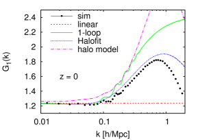
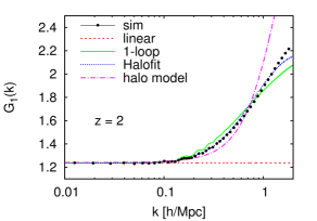
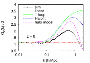
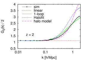
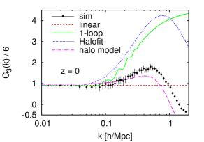
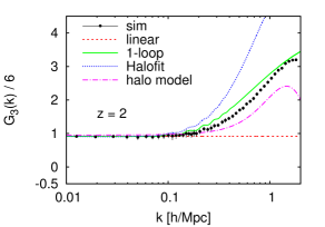
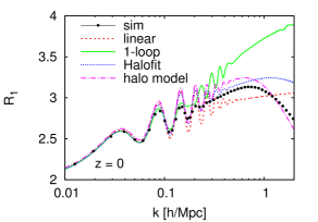
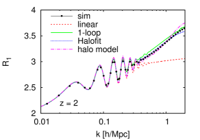
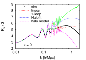
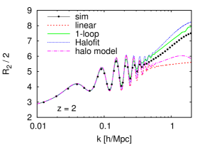
Figure 2 shows the first three growth-only response functions measured from the simulations at $z=0$ (left column) and $z=2$ (right column). These correspond to the fully nonlinear squeezed limit bispectrum (3-point function), trispectrum (4-point function) and 5-point function, and are essentially the same as in figure 2 of Ref. [20], although the results presented there are derived from lower resolution simulations (particle load of $256^{3}$). The small wiggles in the growth-only response functions result from the damping of the baryon acoustic oscillations (BAO), which depends on the amplitude of density fluctuations and thus on $\delta_{L}$.

Let us compare the simulation results to the theoretical predictions discussed in section 2. On sufficiently large scales, the perturbation theory predictions are the most accurate, as expected. At high redshift, the 1-loop predictions best describe the results overall. The 1-loop predictions also show a BAO damping effect. At $z=0$, the growth-only response is captured best by the halofit prescription (in case of $G_{1}$) or the halo model (in case of $G_{2},\,G_{3}$). We see that the halofit prescription describes the simulation results of the linear response well at both redshifts, but performs significantly worse for the higher-order response functions. The BAO damping effect is essentially absent in both halofit and halo model predictions. Overall, none of the models is able to accurately describe the simulation data in the nonlinear regime, with discrepancies at $z=0$ ranging from 20% in the best case to a factor of several. These discrepancies are not surprising given that we are looking at scales beyond the validity of perturbation theory and at higher $N$-point functions for which the semi-analytical approaches were not tuned.

The halo model prediction does not asymptote exactly to the linear result in the $k\to 0$ limit. This is because the 1-halo term asymptotes to a white noise contribution in this limit, and since the 1-halo term contributes to $G_{n}$ due to the dependence of the halo mass function on $\delta_{L}$ (section 2.4), this induces a correction to the linear prediction which contributes on large scales. Physically, this occurs because the halo model does not enforce momentum conservation of the matter density field. This issue can be fixed by introducing a “mass compensation scale” [38].

The halo model predictions can be tuned to better match the simulation results by allowing for a dependence of the halo profiles on the long-wavelength density, which is expected on physical grounds (see also [24]). Specifically, if the the scale radius of halos at fixed mass increases in the presence of a long-wavelength density perturbation, this lowers the peak in the response and thus could lead to better agreement with the simulations results. A detailed investigation of this is beyond the scope of the present paper.

4.2 Comparison to simulations with rescaled initial amplitude

All models for the growth-only response functions that we have presented in section 2 and shown above are based on the approximation that we can trade the effect of $\delta_{L}$ for an appropriate change to the linear growth factor (or equivalently, the linear power spectrum). But how well does this approximation work? Using the set of simulations described in section 3.2, we can explicitly test this approximation on all scales including the nonlinear regime.

In figure 3, we show the growth-only response functions measured from two different sets of simulations. In case of $G_{1}$, this comparison was also shown in figure 6 of [24], and our results agree with theirs. The “rescaled amplitude simulations” of section 3.2 all assume the fiducial cosmology but vary the amplitude of the linear power spectrum used to initialize the simulations so as to match the linear power spectrun in the modified cosmology at the given output times [Eq. (2.14) and Eq. (2.20)]. On linear scales, these simulations thus agree with the “separate universe” simulations by construction. As the simulations share the same random realization of the initial density, the sample variance (noise in the upper panels) gets vastly reduced when considering the difference of the measured response functions, $\Delta G_{n}=G_{n}^{\rm rescaled}-G_{n}^{\rm separate}$. This is shown in the lower subpanels of figure 3, where we have divided $\Delta G_{n}$ by the corresponding linear growth-only response, i.e. the prediction in the $k\to 0$ limit.

The differences seen in figure 3 are caused by the different growth history, which is not captured by the rescaling of the initial amplitude. Following the discussion in section 2.3, the commonly used SPT approach factorizing the growth factor and scale dependence assumes at all orders that a long wavelength density perturbation enters exclusively through the modified linear growth. Thus, even when calculated to all orders, the best that this SPT calculation could do is to reproduce the rescaled amplitude result in figure 3, which deviates from the actual response at $z=0$ by 10% at $k\simeq 0.5\,h\,{\rm Mpc}^{-1}$ and 20% at $k\simeq 1\,h\,{\rm Mpc}^{-1}$ for $G_{1}$, and significantly worse for the higher-order response functions. At $z=2$ on the other hand, the rescaled-amplitude $G_{1}$ matches the separate universe response to better than 10% even beyond $k=1\,h\,{\rm Mpc}^{-1}$, and for $G_{2},\,G_{3}$ performs significantly better as well.

Figure 3: Comparison of the growth-only response functions $G_{1},\,G_{2},\,G_{3}$ (top to bottom) measured at $z=0$ (left column) and $z=2$ (right column) from one realization of the separate universe simulations and from the same realization simulated by varying the initial amplitude. The bottom sub-panels show the difference, $\Delta G_{n}=G_{n}^{\rm rescaled}-G_{n}^{\rm separate}$, divided by the response of the linear matter power spectrum, $G_{n}^{\rm linear}$.

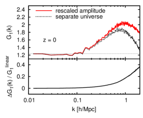
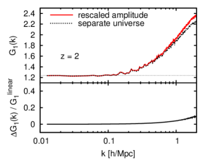
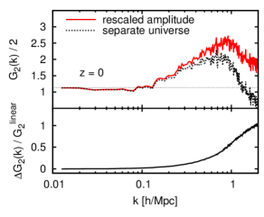
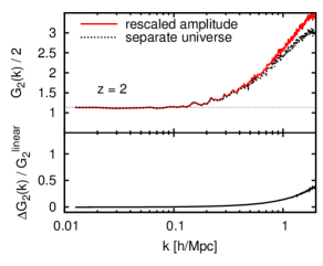
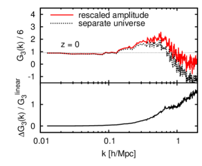
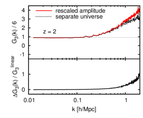
There are two possible explanations for these discrepancies in the SPT context. First, using the SPT kernels derived for an Einstein-de Sitter universe (which have time-independent coefficients), with the $\Lambda$CDM linear growth factor replacing the Einstein-de Sitter $a(t)$, could become highly inaccurate for $\Lambda$CDM at higher orders. Note that the same issue exists for a fiducial flat Einstein-de Sitter universe, since for $\delta_{L}\neq 0$ the quantity $\Omega_{m}/f^{2}$ is no longer 1 (in fact, $d(\Omega_{m}/f^{2})/d\delta_{L}=-5/21$ [14]; see also the discussion in [13]). There is no indication of such a strong effect at low orders in perturbation theory, where this approximation typically performs to better than a percent [27]. Furthermore, ref. [14] found that a cancelation in the curvature contribution to the growth integral suppresses this effect. Finally, ref. [24] shows that the growth-only response of the power spectrum to a change in the Hubble constant while keeping $\Omega_{m}h^{2}$ fixed follows the separate universe response very closely (Fig. 6 there). If the much larger discrepancies between separate universe response and rescaled amplitude response were due to the cosmology dependence of the SPT kernels, one would not expect this to be the case. Nevertheless, we do not claim to be able to rigorously exclude this possibility.

The other possibility, more likely in our opinion, is that the discrepancy between rescaled amplitude and full separate universe simulations is due to effective non-perfect fluid terms, such as pressure and anisotropic stress, in the dark matter fluid [39]. The effective fluid properties depend on highly nonlinear small scales which are not described by the Euler-Poisson system. Their value can depend on the growth history (as well as the power spectrum shape) thus leading to a discrepancy between rescaled amplitude and separate universe simulations. Assuming this interpretation is correct, figure 3 explicitly shows the breakdown of SPT on nonlinear scales as effective pressure, anisotropic stress and sound speed need to be included. Separate universe simulations can be used to measure the response of these effective terms to a long-wavelength overdensity, which is crucial when modeling $(N>2)$-point functions. The results shown in figure 3 are analogous to what has been found for the mass function of halos which is a key ingredient in the halo model description of the nonlinear matter density field. The mass function shows departures from being a simple function of the linear matter power spectrum at the 5–10% level [40, 41].

In an Einstein-de Sitter cosmology with scale-invariant initial power spectrum $P_{l}(k)\propto k^{n}$, there is only one characteristic spatial scale at any given time, which corresponds to the scale at which the density field becomes order 1 [42]. Let us denote this wavenumber as $k_{\rm NL}(t)$. Then, the response functions have to follow a universal function of $k/k_{\rm NL}(t)$, i.e. $G_{m}(k,t)=G_{m}(k/k_{\rm NL})$ (keeping the index of the initial power spectrum fixed). Thus, in this specific case, separate universe simulations and rescaled-amplitude simulations will give exactly the same result when compared at fixed $k/k_{\rm NL}$. The departures shown in figure 3 can thus be seen as a consequence of the $\Lambda$CDM background and the departure from scale-invariance of the initial power spectrum. It would be interesting to disentangle the two effects, e.g. by performing separate universe simulations in $\Lambda$CDM with scale-invariant initial conditions. We leave this for future work, but point out that when plotting the differences shown in the lower panel of figure 3 as a function of $k/k_{\rm NL}$, we still find a factor of several difference in the $z=0$ and $z=2$ results.

Note that in Ref. [38], the authors performed a similar comparison as the one shown for $G_{1}$ in figure 3. However, instead of studying the growth-only response as considered here, they included the reference density effect and found a significantly larger discrepancy between the two measurements considered. As discussed in section 2, however, the reference density effect is a simple remapping, and the growth-only response considered here is the proper quantity to compare for the question we are interested in, namely to measure the effect of the growth history.

Figure 4: The first three full response functions of the power spectrum measured from the separate universe simulations at $z=0$ (left) and $z=2$ (right).

4.3 Full response functions

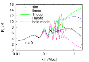
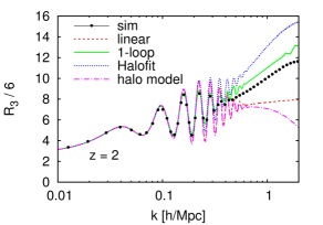
We now turn to the results for the full response functions, i.e. including the “dilation” and “reference density” effects. The results of the simulations and the model predictions are shown in figure 4. The oscillations in the response functions can be traced back to the BAOs in the power spectrum. The BAOs propagate to the response functions primarily by the “dilation” effect, which yields derivatives of the power spectrum with respect to $k$ (see Eqs. (2.10)–(2.12)). The 1-loop perturbation theory predictions describe the simulation results accurately up to $k\leq 0.15\,h^{-1}{\rm Mpc}$ and $k\leq 0.3\,h^{-1}{\rm Mpc}$ at $z=0$ and $z=2$, respectively. As the other theoretical models do not include the damping of the BAOs in the nonlinear power spectrum, they predict oscillations in the response functions which are too large. To improve the accuracy of those models around the BAO scale, one would need to put in the BAO damping by hand. In the nonlinear regime, none of the models is able to reproduce the simulation data. In principle, one could build a hybrid model for the full response by combining an accurate prediction of the nonlinear power spectrum of the fiducial cosmology and the growth-only response functions $G_{n}(k)$ discussed in the previous section. In this paper, however, we do not pursue this approach.

Figure 5: The first three Eulerian response functions of the power spectrum measured from the separate universe simulations (data points) at $z=0$ (left) and $z=2$ (right). The lines show the corresponding linear combinations of the Lagrangian response functions using the $f_{n}$ coefficients derived for the Einstein-de Sitter universe (see Eq. (4.1) and Eq. (B.18)).

4.4 Eulerian response functions

So far, we have always considered the response to the linearly-extrapolated initial (Lagrangian) overdensity $\delta_{L}$. We now consider the corresponding response to the evolved nonlinear (Eulerian) overdensity $\delta_{\rho}$. Using the expansion derived for the Einstein-de Sitter universe, Eq. (B.18), we find

$$R_{1}^{\rm Eulerian}(k) =R_{1}(k)\,,$$

$$R_{2}^{\rm Eulerian}(k) =R_{2}(k)-2f_{2}R_{1}(k)\,,$$

$$R_{3}^{\rm Eulerian}(k) =R_{3}(k)-6f_{2}R_{2}(k)+6\left(2f_{2}^{2}-f_{3}\right)R_{1}(k)\,.$$ (4.1)

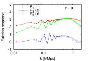
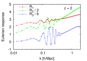
In figure 5, we compare the directly measured Eulerian response functions with the appropriate linear combinations of the measured Lagrangian response functions. The agreement is excellent as expected, especially at high redshift at which the $\Lambda$CDM universe is very well approximated by the Einstein-de Sitter universe.

Interestingly, the higher-order Eulerian response functions are much smaller than in the Lagrangian case. That is, the response of the nonlinear matter power spectrum to a uniform nonlinear final-time density $\delta_{\rho}$ is close to linear. This is most likely due to the fact that the growth-only response functions are subdominant compared to the rescaling and reference density contributions, especially at higher order. In this case, Eq. (2.6) implies a close to linear scaling with $\delta_{\rho}$.

5 Conclusions

In this paper, we employed dedicated N-body simulations using the separate universe technique presented in Ref. [20] to compute the response of the nonlinear matter power spectrum to a homogeneous overdensity superimposed on a flat FLRW universe. The response functions we computed give the squeezed limits of the 3-, 4-, and 5-point functions, in which all but two wavenumbers are taken to be small and are angle-averaged. By virtue of the separate universe technique, we reach an unprecedented accuracy of these nonlinear matter $N$-point functions.

The response function consists of three parts: changing the reference density with respect to which the power spectrum is defined; rescaling of comoving coordinates; and the effect on the growth of structure. The former two effects can be calculated trivially, whereas the third one requires separate universe simulations. We have compared the simulation results with analytical and semi-analytical results, in particular standard perturbation theory (SPT), the empirical fitting function halofit, and the halo model, finding that SPT typically yields the best results at high redshifts. The fitting function and halo model, while qualitatively describe the trends seen in the response functions, give a poor quantitative description on nonlinear scales.

A fundamental assumption of all of the analytical and semi-analytical methods used in this paper, including standard perturbation theory at any order, is that nonlinear matter statistics at a given time are given solely by the linear power spectrum at the same time, and do not depend on the growth history otherwise. As was done in [24] for the response function for $n=1$, we were able to test this assumption for $n=2$ and 3 quantitatively by comparing the separate universe simulations with simulations with a rescaled initial power spectrum amplitude. We find that this assumption fails at the level of 10% at $k\simeq 0.2-0.5\,h\,{\rm Mpc}^{-1}$ for $5$- to $3$-point functions at $z=0$. The failure occurs at higher wavenumbers at $z=2$. In the context of SPT, this may signal a breakdown of the perfect fluid description of the dark matter density field at and beyond these wavenumbers. In other words, even if computed to all orders, SPT (and its variants such as RPT [28]) fails to describe the nonlinear structure formation beyond these wavenumbers. Therefore, our results yields a quantitative estimate for the scales at which effective fluid corrections become important in the bispectrum and higher $N$-point functions, and at which one should stop trusting pure SPT calculations.

Finally, we point out that the approach presented here can be augmented to measure more general squeezed-limit $N$-point functions, by including the response to long-wavelength tidal fields and by considering the response of small-scale $n$-point functions in addition to the small-scale power spectrum considered here.

Appendix A Squeezed limit $N$-point functions and power spectrum response

In this appendix, we prove the relation Eq. (1.2) between the power spectrum response and the squeezed limit $N$-point functions. We only consider equal-time $N$-point functions, to which there are no boost-type contributions from kinematical consistency relations. Further, we assume that the long-wavelength modes are well inside the horizon, removing gauge-dependent terms present for horizon-scale modes. Note that the relations derived here retain their formal validity even for horizon-scale long-wavelength modes if the matter density perturbation is evaluated in synchronous-comoving gauge [16].

As in Eq. (1.3), we expand the power spectrum as a function of the linearly extrapolated initial overdensity $\delta_{L0}$ as

$$P(k,t|\delta_{L0})=\sum_{n=0}^{\infty}\frac{1}{n!}R_{n}(k,t)\left[\delta_{L0}\hat{D}(t)\right]^{n}\>P(k,t)\,,$$ (A.1)

where $R_{n}(k,t)$ are response functions with $R_{0}(k,t)=1$. At the same order in derivatives, that is at the same order in $k_{i}/k$ of the squeezed-limit $N$-point function, the power spectrum will also depend on the long-wavelength tidal field which can be parametrized through

$$K_{ij}(\mathbf{k})\equiv\left(\frac{k_{i}k_{j}}{k^{2}}-\frac{1}{3}\delta_{ij}\right)\delta(\mathbf{k})\,.$$ (A.2)

Exploring the response of the power spectrum to a long-wavelength tidal field is beyond the scope of this paper. We remove the dependence on $K_{ij}$ by performing an angle-average of the long-wavelength modes which cancels the tidal field contributions.

In the following, we will suppress the time argument for clarity. We let $\mathcal{S}_{n}$ be defined as in Eq. (1.1),

$$\mathcal{S}_{n}(k,k^{\prime};k_{1},\cdots,k_{n})\equiv\> \int\frac{d^{2}\hat{\mathbf{k}}_{1}}{4\pi}\cdots\int\frac{d^{2}\hat{\mathbf{k}}_{n}}{4\pi}\left\langle\delta(\mathbf{k})\delta(\mathbf{k}^{\prime})\delta(\mathbf{k}_{1})\cdots\delta(\mathbf{k}_{n})\right\rangle^{\prime}_{c}\,.$$ (A.3)

Here, the prime denotes that the factor $(2\pi)^{3}\delta_{D}(\mathbf{k}+\mathbf{k}^{\prime}+\mathbf{k}_{1\cdots n})$ is dropped, where $\mathbf{k}_{1\cdots n}=\sum_{i=1}^{n}\mathbf{k}_{i}$. We consider the limit

$$\lim_{k_{i}\to 0}\;\frac{\mathcal{S}_{n}(k,k^{\prime};k_{1},\cdots k_{n})}{P(k)P_{l}(k_{1})\cdots P_{l}(k_{n})}\,,$$ (A.4)

which means that all $|\mathbf{k}_{i}|$ are taken to zero. In this limit, spatial homogeneity enforces $\mathbf{k}^{\prime}=-\mathbf{k}+\mathcal{O}(k_{i}/k)$, so that (for statistically isotropic initial conditions) the r.h.s. only depends on $k$.

In order to prove Eq. (1.2), we first note that since we are interested in the limit $k_{i}\to 0$, we can replace $\delta(\mathbf{k}_{i})$ in Eq. (1.1) with the linear density field $\delta_{L}(\mathbf{k}_{i})$. We further transform $\mathbf{k}_{i}$ into real space, writing

$$\mathcal{S}_{n}(k;k_{1},\cdots,k_{n})=\> \int\frac{d^{2}\hat{\mathbf{k}}_{1}}{4\pi}\cdots\int\frac{d^{2}\hat{\mathbf{k}}_{n}}{4\pi}\prod_{i=1}^{n}\int d^{3}\mathbf{x}_{i}\>e^{i\mathbf{x}_{i}\cdot\mathbf{k}_{i}}\left\langle\delta(\mathbf{k})\delta(\mathbf{k}^{\prime})\delta(\mathbf{x}_{1})\cdots\delta(\mathbf{x}_{n})\right\rangle^{\prime}_{c}$$

$$=\> \prod_{i=1}^{n}\int d^{3}\mathbf{x}_{i}\>e^{i\mathbf{x}_{i}\cdot\mathbf{k}_{i}}\>\tilde{\mathcal{S}}_{n}(k,x_{1},\cdots x_{n})\,,$$ (A.5)

where

$$\tilde{\mathcal{S}}_{n}(k;x_{1},\cdots x_{n})\equiv\int\frac{d^{2}\hat{\mathbf{x}}_{1}}{4\pi}\cdots\int\frac{d^{2}\hat{\mathbf{x}}_{n}}{4\pi}\left\langle\delta(\mathbf{k})\delta(\mathbf{k}^{\prime})\delta(\mathbf{x}_{1})\cdots\delta(\mathbf{x}_{n})\right\rangle^{\prime}_{c}\,,$$ (A.6)

Note that the angle average is a linear operation and thus commutes with the Fourier transform; in other words, the $k$-space angle average of the Fourier transform of a function is the Fourier transform of the $x$-space angle average of the same function.

Now consider the limit $k_{i}\to 0$, which implies that $x_{i}\to\infty$ in the argument of $\tilde{\mathcal{S}}_{n}$. Then $\tilde{\mathcal{S}}_{n}(k)$ describes the modulation of the small-scale power spectrum $P(k,\mathbf{0})$ measured around $\mathbf{x}=0$ by $n$ spherically symmetric large-scale modes (recall that $\mathbf{k}^{\prime}\approx-\mathbf{k}$). This statement can be formalized by introducing an intermediate scale $R_{L}$ such that $1/k\ll R_{L}\ll|\mathbf{x}_{i}|\sim 1/k_{i}$ and defining $\delta(\mathbf{k})\to\delta_{R_{L}}(\mathbf{k})$ to be the Fourier transform within a cubic volume of size $R_{L}$ around $\mathbf{x}=0$. Then, $\delta_{R_{L}}(\mathbf{k})=\delta(\mathbf{k})+\mathcal{O}(1/(kR_{L}))$, while the long-wavelength modes are constant over the same volume with corrections suppressed by $k_{i}R_{L}$. The corrections we expect in the end are thus of order $k_{i}/k$. To lowest order in these corrections, $\tilde{\mathcal{S}}_{n}(k)$ can be written as

$$\lim_{k_{i}\to 0}:\quad\tilde{\mathcal{S}}_{n}(k;x_{1},\cdots x_{n})=\> \int\frac{d^{2}\hat{\mathbf{x}}_{1}}{4\pi}\cdots\int\frac{d^{2}\hat{\mathbf{x}}_{n}}{4\pi}\left\langle P(k,\mathbf{0})\delta_{L}(\mathbf{x}_{1})\cdots\delta_{L}(\mathbf{x}_{n})\right\rangle^{\prime}_{c}\,.$$ (A.7)

We can now insert the expression for the local power spectrum from Eq. (A.1), which immediately yields

$$\lim_{k_{i}\to 0}:\quad\tilde{\mathcal{S}}_{n}(k;x_{1},\cdots x_{n})=\> \sum_{m=0}^{\infty}\frac{1}{m!}R_{m}(k)P(k)\int\frac{d^{2}\hat{\mathbf{x}}_{1}}{4\pi}\cdots\int\frac{d^{2}\hat{\mathbf{x}}_{n}}{4\pi}\left\langle\delta_{L}^{m}(\mathbf{0})\delta_{L}(\mathbf{x}_{1})\cdots\delta_{L}(\mathbf{x}_{n})\right\rangle^{\prime}_{i-0}\,.$$ (A.8)

Here, the subscript $i-0$ indicates that only contractions between $\mathbf{0}$ and $\mathbf{x}_{i}$ are to be taken, since the l.h.s. is defined through the connected correlation function (all other contractions would contribute to the disconnected part of $\left\langle\delta(\mathbf{k})\delta(\mathbf{k}^{\prime})\delta(\mathbf{x}_{1})\cdots\delta(\mathbf{x}_{n})\right\rangle$). Since all density fields in the correlator in Eq. (A.8) are linear, limiting to the contractions between $\mathbf{0}$ and $\mathbf{x}_{i}$ then constrains $m=n$. We obtain

$$\lim_{k_{i}\to 0}:\quad\tilde{\mathcal{S}}_{n}(k;x_{1},\cdots x_{n})=\> \frac{1}{n!}R_{n}(k)P(k)\>n!\prod_{i=1}^{n}\int\frac{d^{2}\hat{\mathbf{x}}_{i}}{4\pi}\>\xi_{L}(\mathbf{x}_{i})$$

$$=\> R_{n}(k)P(k)\prod_{i=1}^{n}\int\frac{d^{3}\mathbf{k}_{i}}{(2\pi)^{3}}e^{i\mathbf{x}_{i}\cdot\mathbf{k}_{i}}P_{L}(k_{i})\,.$$ (A.9)

Here, $\xi_{L}$ and $P_{L}$ denote the linear matter correlation function and power spectrum, respectively. The angle average in the first line is trivial of course. Going back to Fourier space then immediately yields that for $k_{i}\to 0$,

$$\mathcal{S}_{n}(k;k_{1},\cdots k_{n})=R_{n}(k)P(k)\prod_{i=1}^{n}P_{L}(k_{i})+\mathcal{O}\left(\frac{k_{i}}{k},\>\frac{k_{i}}{k_{\rm NL}}\right)\,,$$ (A.10)

where $k_{\rm NL}$ is the nonlinear scale. This can be reordered to yield Eq. (1.2),

$$R_{n}(k)=\lim_{k_{i}\to 0}\;\frac{\mathcal{S}_{n}(k;k_{1},\cdots k_{n})}{P(k)P_{L}(k_{1})\cdots P_{L}(k_{n})}\,.$$

This provides the connection between the response functions $R_{n}(k)$ and the angle-averaged matter $(n+2)$-point function Eq. (1.1) in a certain limit squeezed limit (since $k_{i}\ll k$). Note that no assumption about the magnitude of $k$ has been made, i.e. this value can be fully nonlinear. In this paper, we accurately determine this fully nonlinear quantity using simulations. In the following subsections, we illustrate Eq. (1.2) at tree level in perturbation theory for the cases $n=1$ (three-point function) and $n=2$ (four-point function).

A.1 Tree-level result: $n=1$

At tree-level for $n=1$ we obtain

$$\lim_{k_{i}\to 0}\mathcal{S}_{1}(k;k_{1})\stackrel{{\scriptstyle\rm tree-level}}{{=}}\> 2\lim_{k_{1}\to 0}\>\int\frac{d^{2}\hat{\mathbf{k}}_{1}}{4\pi}\left[F_{2}(\mathbf{k},\mathbf{k}_{1})P_{l}(k)+F_{2}(-\mathbf{k}-\mathbf{k}_{1},\mathbf{k}_{1})P_{l}(|\mathbf{k}+\mathbf{k}_{1}|)\right]P_{l}(k_{1})\,.$$ (A.11)

Eq. (1.2) then yields

$$R_{1}(k)\stackrel{{\scriptstyle\rm tree-level}}{{=}}\frac{2}{P_{l}(k)}\lim_{k_{1}\to 0}\>\int\frac{d^{2}\hat{\mathbf{k}}_{1}}{4\pi}\left[F_{2}(\mathbf{k},\mathbf{k}_{1})P_{l}(k)+F_{2}(-\mathbf{k}-\mathbf{k}_{1},\mathbf{k}_{1})P_{l}(|\mathbf{k}+\mathbf{k}_{1}|)\right]\,.$$ (A.12)

where

$$F_{2}(\mathbf{k},\mathbf{k}_{1})=\frac{5}{7}+\frac{1}{2}\mu\left(\frac{k}{k_{1}}+\frac{k_{1}}{k}\right)+\frac{2}{7}\mu^{2}\,,$$ (A.13)

where $\mu$ is the cosine of $\mathbf{k}$ and $\mathbf{k}_{1}$. The term $\mu/2(k/k_{1})$ is problematic as we are sending $k_{1}\to 0$. Using that

$$|\mathbf{k}+\mathbf{k}_{1}|=\> k(1+q\mu+\mathcal{O}(q^{2})),\quad q=\frac{k_{1}}{k}$$

$$P_{l}(|\mathbf{k}+\mathbf{k}_{1}|)=\> P_{l}(k)\left[1+\frac{d\ln P_{l}(k)}{d\ln k}q\mu+\mathcal{O}(q^{2})\right]\,,$$ (A.14)

the sum of the two IR-divergent terms in Eq. (A.12) becomes

$$\frac{1}{2}\left\{\mu\frac{k}{k_{1}}P_{l}(k)+\frac{-(\mathbf{k}+\mathbf{k}_{1})\cdot\mathbf{k}_{1}}{|\mathbf{k}+\mathbf{k}_{1}|k_{1}}P_{l}(|\mathbf{k}+\mathbf{k}_{1}|)\right\}=\frac{1}{2}P_{l}(k)\left[-\mu^{2}\frac{d\ln P_{l}(k)}{d\ln k}-1\right]+\mathcal{O}(q)\,.$$ (A.15)

As expected, the divergent pieces have canceled. We have dropped terms of order $k_{1}/k$ which are irrelevant in the limit we are interested in. We finally obtain

$$R_{1}(k)\stackrel{{\scriptstyle\rm tree-level}}{{=}}\> 2\int_{-1}^{1}\frac{d\mu}{2}\left[\frac{10}{7}-\frac{1}{2}\left(\mu^{2}\frac{d\ln P_{l}}{d\ln k}+1\right)+\frac{4}{7}\mu^{2}\right]$$

$$=\> 2\left[\frac{10}{7}-\frac{1}{6}\frac{d\ln P_{l}}{d\ln k}-\frac{1}{2}+\frac{4}{21}\right]=\frac{47}{21}-\frac{1}{3}\frac{d\ln P_{l}}{d\ln k}\,.$$ (A.16)

This agrees with the linear prediction for $R_{1}$, obtained from substituting $f_{1}$, $e_{1}$, and $g_{1}$ into Eq. (2.10).

A.2 Tree-level result: $n=2$

At $n=2$, we have

$$\mathcal{S}_{n}(k;k_{1},k_{2})=\> \int\frac{d^{2}\hat{\mathbf{k}}_{1}}{4\pi}\int\frac{d^{2}\hat{\mathbf{k}}_{2}}{4\pi}\left\langle\delta(\mathbf{k})\delta(\mathbf{k}^{\prime})\delta(\mathbf{k}_{1})\delta(\mathbf{k}_{2})\right\rangle^{\prime}_{c}$$

$$\stackrel{{\scriptstyle k_{1},k_{2}\to 0}}{{=}}\> \int\frac{d^{2}\hat{\mathbf{k}}_{1}}{4\pi}\int\frac{d^{2}\hat{\mathbf{k}}_{2}}{4\pi}\Bigg{\{}6\Big{[}F_{3}(\mathbf{k},\mathbf{k}_{1},\mathbf{k}_{2})P_{l}(k)$$

$$+F_{3}(-\mathbf{k}-\mathbf{k}_{12},\mathbf{k}_{1},\mathbf{k}_{2})P_{l}(|\mathbf{k}+\mathbf{k}_{12}|)\Big{]}$$

$$+4\Big{[}F_{2}(-\mathbf{k}_{1},\mathbf{k}+\mathbf{k}_{1})F_{2}(\mathbf{k}_{2},\mathbf{k}+\mathbf{k}_{1})P_{l}(|\mathbf{k}+\mathbf{k}_{1}|)$$

$$+F_{2}(\mathbf{k}_{1},\mathbf{k}+\mathbf{k}_{2})F_{2}(-\mathbf{k}_{2},\mathbf{k}+\mathbf{k}_{2})P_{l}(|\mathbf{k}+\mathbf{k}_{2}|)\Big{]}\Bigg{\}}P_{l}(k_{1})P_{l}(k_{2})\,,$$ (A.17)

where $F_{3}$ is the symmetrized third-order perturbation theory kernel, and the unsymmetrized form can be found in [43]. Both $F_{2}^{2}$ and $F_{3}$ contain formally IR-divergent terms up to $\mathcal{O}[(q_{1,2})^{2}]$ where $q_{1,2}=k_{1,2}/k$ for $k_{1,2}\to 0$ which cancel in the end, so we should expand the power spectrum to $\mathcal{O}[(k_{1,2})^{2}]$ to obtain the consistent result at order $\mathcal{O}[(q_{1,2})^{0}]$. We have

$$P_{l}(|\mathbf{k}+\mathbf{k}_{1}|)=\> P_{l}(k)\left[1+\left(q_{1}\mu_{1}+\frac{q_{1}^{2}}{2}[1-\mu_{1}^{2}]\right)\frac{k}{P_{l}(k)}\frac{dP_{l}(k)}{dk}+\frac{q_{1}^{2}\mu_{1}^{2}}{2}\frac{k^{2}}{P_{l}(k)}\frac{d^{2}P_{l}(k)}{dk^{2}}+\mathcal{O}(q_{1}^{3})\right]$$

$$P_{l}(|\mathbf{k}+\mathbf{k}_{1}+\mathbf{k}_{2}|)=\> P_{l}(k)\Bigg{[}1+\Big{(}[q_{1}\mu_{1}+q_{2}\mu_{2}]+\frac{1}{2}\big{[}q_{1}^{2}(1-\mu_{1}^{2})+q_{2}^{2}(1-\mu_{2}^{2})$$

$$+2q_{1}q_{2}(\mu_{12}-\mu_{1}\mu_{2})\big{]}\Big{)}\frac{k}{P_{l}(k)}\frac{dP_{l}(k)}{d\ln k}$$

$$+\frac{1}{2}\left(q_{1}^{2}\mu_{1}^{2}+q_{2}^{2}\mu_{2}^{2}+2q_{1}q_{2}\mu_{1}\mu_{2}\right)\frac{k^{2}}{P_{l}(k)}\frac{d^{2}P_{l}(k)}{dk^{2}}+\mathcal{O}[(q_{1,2})^{3}]\Bigg{]}\,,$$ (A.18)

where $\mu_{1,2}$ is the cosine of $\mathbf{k}$ and $\mathbf{k}_{1,2}$, and $\mu_{12}$ is the cosine of $\mathbf{k}_{1}$ and $\mathbf{k}_{2}$. The leading order terms are

$$R_{2}(k)\stackrel{{\scriptstyle\rm tree-level}}{{=}}\> \int\frac{d^{2}\hat{\mathbf{k}}_{1}}{4\pi}\int\frac{d^{2}\hat{\mathbf{k}}_{2}}{4\pi}\frac{1}{147}\Bigg{[}(628+324\mu_{1}^{2}+112\mu_{12}^{2}$$

$$-280\mu_{1}\mu_{2}\mu_{12}+380\mu_{2}^{2}+656\mu_{1}^{2}\mu_{2}^{2}-56\mu_{2}^{2}\mu_{12}^{2})$$

$$+(-273\mu_{1}^{2}+147\mu_{1}\mu_{2}\mu_{12}-336\mu_{2}^{2}-483\mu_{1}^{2}\mu_{2}^{2}+63\mu_{2}^{2}\mu_{12}^{2})\frac{k}{P_{l}(k)}\frac{dP_{l}(k)}{dk}$$

$$+147\mu_{1}^{2}\mu_{2}^{2}\frac{k^{2}}{P_{l}(k)}\frac{d^{2}P_{l}(k)}{dk^{2}}\Bigg{]}$$

$$=\> \frac{8420}{1323}-\frac{100}{63}\frac{k}{P_{l}(k)}\frac{dP_{l}(k)}{dk}+\frac{1}{9}\frac{k^{2}}{P_{l}(k)}\frac{d^{2}P_{l}(k)}{dk^{2}}\,,$$ (A.19)

which is in agreement with the linear prediction of Eq. (2.11) once the numbers for $e_{i},\,f_{i},\,g_{i}$ $(i=1,2)$ are inserted.

Appendix B Analytical solution for $\delta_{\rho}$ and $\delta_{a}$ in Einstein-de Sitter

As derived in [20], the modified cosmology described by $\tilde{a}(t)$ follows the evolution equation of a uniform density spherical perturbation in the fiducial cosmology. In this section, we take the fiducial cosmology to be Einstein-de Sitter (EdS), $\Omega_{m}=1$, and consider a positive overdensity perturbation. In this case there is a well known parametric solution for the collapse [44]:

$$\tilde{a}(\theta)=\> \frac{1}{2}\frac{\tilde{\Omega}_{m}}{\tilde{\Omega}_{m}-1}(1-\cos\theta)$$

$$\tilde{H}_{0}t(\theta)=\> \frac{1}{2}\frac{\tilde{\Omega}_{m}}{(\tilde{\Omega}_{m}-1)^{3/2}}(\theta-\sin\theta)\,.$$ (B.1)

Note that $\tilde{\Omega}_{m}-1=-\tilde{\Omega}_{K}>0$. We now want to derive the matching between $\tilde{H}_{0}$ and $\tilde{\Omega}_{m}$ with the fiducial values and the linearly extrapolated overdensity $\delta_{L0}$. The same matching also works for $\delta_{L0}<0$ in which case the $\sin,\,\cos$ are to be replaced by $\sinh,\,\cosh$. First, the $\theta\to 0$ limit should reduce to EdS, where

$$\tilde{a}(t)=\left(\frac{3}{2}\tilde{H}_{0}t\right)^{2/3}\,,$$ (B.2)

so that $\tilde{a}(t_{0})=1$ and $\tilde{H}(t_{0})=\dot{\tilde{a}}(t_{0})/\tilde{a}(t_{0})=\tilde{H}_{0}$. One can further expand Eq. (B.1) around $\theta=0$. On the other hand, we know the linear relation between $\tilde{a}(t)$ and $a(t)$, since at linear order $\delta_{a}=-\delta_{\rho}/3=-\delta_{L0}a(t)/3$:

$$\tilde{a}(t)=a(t)[1+\delta_{a}(t)]=\left(\frac{3}{2}H_{0}t\right)^{2/3}\left[1-\frac{1}{3}\delta_{L0}\left(\frac{3}{2}H_{0}t\right)^{2/3}\right]\,,$$ (B.3)

where we have used that $a(t_{0})=1$ and $\delta_{L0}$ is the linearly extrapolated overdensity at $t_{0}$. Matching at zeroth order in $(H_{0}t)^{2/3}$ yields an identity. At linear order in $\delta_{L0}$, we obtain

$$\frac{\tilde{\Omega}_{m}-1}{\tilde{\Omega}_{m}}=\> \frac{5}{3}\delta_{L0}\quad\mbox{and}\quad 1-(1+\delta_{H})^{2}=\frac{5}{3}\delta_{L0}\,,$$ (B.4)

where $1+\delta_{H}=\tilde{H}_{0}/H_{0}$. Thus, we have determined all quantities in Eq. (B.1) in terms of $\delta_{L0}$.

One might wonder what happens in the limit $\delta_{L0}\to 3/5$, which implies $\tilde{K}/H_{0}^{2}\to 1$, $\tilde{\Omega}_{m}\to\infty$ and $\delta_{H}\to-1$ and thus seemingly an ill-defined cosmology. Let us investigate the solution Eq. (B.1) in this limit. First, we have

$$H_{0}t(\theta)=\> \frac{1}{2}\frac{(1+\delta_{H})^{-3}}{(\tilde{\Omega}_{m}-1)^{3/2}}(\theta-\sin\theta)=\frac{1}{2}\left(1-(1+\delta_{H})^{2}\right)^{-3/2}(\theta-\sin\theta)\,.$$

For $\delta_{H}\to-1$ and $\tilde{\Omega}_{m}\to\infty$, this solution becomes

$$\tilde{a}(\theta)=\> \frac{1}{2}(1-\cos\theta)$$

$$H_{0}t(\theta)=\> \frac{1}{2}(\theta-\sin\theta)\,.$$ (B.6)

Thus, the solution remains perfectly valid. It is simply the parametrization in terms of $\tilde{H}_{0}$ and $\tilde{\Omega}_{m}$ which breaks down. We also see why this happens: turn-around happens in Eq. (B.6) at $\theta=\pi$, $H_{0}t_{\rm ta}=\pi/2$, and $a_{\rm ta}=1$. Thus, the Hubble constant goes to zero just at the point where we are trying to match the Friedmann equation, which of course assumes an expanding universe. For even larger overdensities, $a(\theta)$ never reaches unity and thus no matching to $\tilde{H}_{0},\>\tilde{\Omega}_{m}$ is possible. Note that solutions of course exist, they are simply not captured by a parametrization of the form Eq. (B.1). In any case, such large nonperturbative values of the long-wavelength overdensity are not of practical interest for the application to separate universe simulations.

B.1 Perturbative solution and nonlinear growth factor

In this section we derive the series solution Eq. (2.7) for $\delta_{a}$ and $\delta_{\rho}$ in EdS. We write the parametric solution as

$$\tilde{a}(\theta)=\> \frac{1}{2}\epsilon^{-1}(1-\cos\theta)$$

$$\hat{t}(\theta)\equiv\frac{t(\theta)}{t_{0}}=\> \frac{3}{4}\epsilon^{-3/2}(\theta-\sin\theta)\,,$$ (B.7)

where we have used $a(t)=(t/t_{0})^{2/3}$, $t_{0}=2/(3H_{0})$, and defined

$$\epsilon\equiv\frac{\tilde{\Omega}_{m}-1}{\tilde{\Omega}_{m}}=\frac{5}{3}\delta_{L0}\,.$$ (B.8)

Our goal is to obtain

$$\tilde{a}(t_{0})=1+\delta_{a}(t_{0})\,.$$ (B.9)

Thus, we need to solve

$$1=\hat{t}(\theta_{0})\quad\Leftrightarrow\quad\frac{4}{3}\epsilon^{3/2}=\theta_{0}-\sin\theta_{0}$$ (B.10)

for $\theta_{0}$. We perform a series expansion,

$$\theta_{0}-\sin\theta_{0}=\frac{1}{6}\theta_{0}^{3}-\frac{1}{120}\theta_{0}^{5}+\cdots=\sum_{n=1}^{\infty}b_{n}\theta_{0}^{2n+1}\,,$$ (B.11)

and solve Eq. (B.10) order by order. The leading solution is $\theta_{0}^{(1)}=2\epsilon^{1/2}$. The $n$-th order solution has to solve

$$\frac{4}{3}\epsilon^{3/2}=\sum_{k=1}^{n}b_{k}\left[\theta_{0}^{(n-k+1)}\right]^{2k+1}\,.$$ (B.12)

Note that in order to trust the final expression at order $\delta_{L0}^{m}$, this solution needs to be expanded to order $n=m+2$. In the following, we choose $m=5$. Solving this order by order, we obtain

$$\theta_{0}=2\epsilon^{1/2}\left[1+\frac{1}{15}\epsilon+\frac{2}{175}\epsilon^{2}+\frac{4}{1575}\epsilon^{3}+\frac{43}{67375}\epsilon^{4}+\cdots\right]\,.$$ (B.13)

We then insert this into $\tilde{a}(\theta)$ and expand in $\epsilon$, replacing $\epsilon$ with $5/3\>\delta_{L0}$ through Eq. (B.8). This yields

$$1+\delta_{a}(t_{0})=\tilde{a}(\theta_{0})=1+\sum_{n=1}^{\infty}e_{n}\delta_{L0}^{n}\,,$$ (B.14)

where the first few coefficients are

$$e_{1}=-\frac{1}{3};\quad e_{2}=-\frac{1}{21};\quad e_{3}=-\frac{23}{1701};\quad e_{4}=-\frac{1894}{392931};\quad e_{5}=-\frac{3293}{1702701}\,.$$ (B.15)

We can generalize this to other times $t$ by replacing $\delta_{L0}$ with $\delta_{L0}a(t)$, which is possible since EdS is scale free:

$$\delta_{a}(t)=\sum_{n=1}^{\infty}e_{n}[\delta_{L0}a(t)]^{n}\,.$$ (B.16)

Finally, we obtain the density at $t$ through

$$\delta_{\rho}(t)=[1+\delta_{a}(t)]^{-3}-1\,,$$ (B.17)

and expanding in powers of $\delta_{L0}$. This yields

$$\delta_{\rho}(t)=\> \sum_{n=1}^{\infty}f_{n}[\delta_{L0}a(t)]^{n}$$

$$f_{1}=\> 1;\quad f_{2}=\frac{17}{21};\quad f_{3}=\frac{341}{567};\quad f_{4}=\frac{55805}{130977};\quad f_{5}=\frac{213662}{729729}\,.$$ (B.18)

We have verified that Eq. (B.16) and Eq. (B.18) are accurate in $\Lambda$CDM as well when replacing $a(t)$ with $D(t)/D(t_{0})$, where $D(t)$ is the growth factor in the fiducial cosmology.

Appendix C Linear growth in modified cosmology

In this section we iteratively solve the growth factor $\tilde{D}(t)$ in the modified cosmology, for a fiducial EdS background, to obtain a perturbative expansion in terms of $\delta_{L0}$ [Eq. (2.14)]. The modified cosmology is described by

$$\tilde{H}^{2}(\tilde{a})=\> \tilde{H}_{0}^{2}\left[\tilde{\Omega}_{m}\tilde{a}^{-3}+(1-\tilde{\Omega}_{m})\tilde{a}^{-2}\right]$$

$$=\> H_{0}^{2}\left[\tilde{a}^{-3}-\epsilon\tilde{a}^{-2}\right]\,,$$ (C.1)

where $\epsilon$ is defined in Eq. (B.8) and we have used $\tilde{\Omega}_{m}\tilde{H}_{0}^{2}=\Omega_{m}H_{0}^{2}=H_{0}^{2}$. Similarly, the mean background density in the curved universe is given by

$$4\pi G\tilde{\bar{\rho}}(t)=\frac{3}{2}\tilde{\Omega}_{m}\tilde{H}_{0}^{2}\tilde{a}^{-3}(t)=\frac{3}{2}H_{0}^{2}\tilde{a}^{-3}(t)\,.$$ (C.2)

On the other hand, in the background EdS cosmology we have

$$H(a)=H_{0}a^{-3/2}\,.$$ (C.3)

We want to derive the growth of density perturbations $\tilde{\delta}_{s}=\rho/\tilde{\bar{\rho}}-1$, where the subscript $s$ denotes that they are small-scale fluctuations, in order to distinguish from the density perturbations $\delta_{\rho}=\tilde{\bar{\rho}}/\bar{\rho}-1$ with respect to the EdS background. Note also that $\delta_{s}$ is defined with respect to the background density of the curved universe (i.e. we do not include the “reference density” contribution here). The growth equation is then given by

$$\ddot{\tilde{\delta}}_{s}+2\tilde{H}(t)\dot{\tilde{\delta}}_{s}-4\pi G\tilde{\bar{\rho}}(t)\tilde{\delta}_{s}=0\,,$$ (C.4)

which becomes

$$\ddot{\tilde{\delta}}_{s}+2H_{0}(\tilde{a}^{-3}-\epsilon\tilde{a}^{-2})^{1/2}\dot{\tilde{\delta}}_{s}-\frac{3}{2}H_{0}^{2}\tilde{a}^{-3}\tilde{\delta}_{s}=\> 0$$

$$\ddot{\tilde{\delta}}_{s}+2H_{0}\tilde{a}^{-3/2}(1-\epsilon\tilde{a})^{1/2}\dot{\tilde{\delta}}_{s}-\frac{3}{2}H_{0}^{2}\tilde{a}^{-3}\tilde{\delta}_{s}=\> 0\,.$$ (C.5)

Note that we have neglected the curvature contribution to the Poisson equation, which involves $3K\Phi$ and the curved-space Laplacian. If $\tilde{K}/H_{0}^{2}\sim 1$, these terms only become relevant for small-scale modes that are of order the horizon. Since we are studying the subhorizon evolution of small-scale modes, and moreover we always have $\tilde{K}/H_{0}^{2}\ll 1$ for a flat fiducial cosmology, these terms are entirely negligible for our purposes. We now replace $t$ with $y=\ln a(t)$ as time coordinate, where $a(t)$ is the scale factor in the EdS background. Dividing by $H^{2}$, and inserting $\epsilon=5/3\delta_{L0}$, we obtain

$$\frac{d^{2}}{dy^{2}}\tilde{\delta}_{s}+\left[2\Delta_{a}^{-3/2}\left(1-\frac{5}{3}\delta_{L0}a\Delta_{a}\right)^{1/2}-\frac{3}{2}\right]\frac{d}{dy}\tilde{\delta}_{s}-\frac{3}{2}\Delta_{a}^{-3}\tilde{\delta}_{s}=0\,,$$ (C.6)

where we have defined $\Delta_{a}(t)\equiv 1+\delta_{a}(t)$. So far, everything is exact. We now perform a series expansion of Eq. (C.6) in $\delta_{L0}$. At zeroth order, $\Delta_{a}=1$, and we obtain

$$\frac{d^{2}}{dy^{2}}\tilde{\delta}_{s}^{(0)}+\frac{1}{2}\frac{d}{dy}\tilde{\delta}_{s}^{(0)}-\frac{3}{2}\tilde{\delta}_{s}^{(0)}=0\,,$$ (C.7)

which has growing and decaying modes of $\tilde{\delta}_{s}^{(0)}\propto e^{y}$ and $e^{-3y/2}$. Thus, it is identical to the growth in the background EdS cosmology, as expected. In the following, we will drop the decaying mode following standard practice. Further, we will normalize $\tilde{\delta}_{s}^{(0)}$ to $a(t)=e^{y}$ at early times, and replace it with $\tilde{D}$ to denote the small-scale growth factor. Thus, $\tilde{D}^{(0)}(t)=a(t)$.

The series expansion of $\Delta_{a}$ is given in Eq. (B.16), which we can generalize to other times $t$ by replacing $\delta_{L0}$ with $\delta_{L0}a(t)$. We see that Eq. (C.6) can be expanded into a series in powers of $\delta_{L0}a$, leading to

$$\frac{d^{2}}{dy^{2}}\tilde{D}+\left[\sum_{m=0}^{\infty}c_{m}\delta_{L0}^{m}e^{my}\right]\frac{d}{dy}\tilde{D}-\left[\sum_{m=0}^{\infty}d_{m}\delta_{L0}^{m}e^{my}\right]\tilde{D}=0\,,$$ (C.8)

with coefficients $c_{m},\>d_{m}$. Specifically, the coefficients are defined through

$$2\Delta_{a}^{-3/2}\left(1-\frac{5}{3}\delta_{L0}a\Delta_{a}\right)^{1/2}-\frac{3}{2}=\> \sum_{m=0}^{\infty}c_{m}[\delta_{L0}a(t)]^{m}$$

$$\frac{3}{2}\Delta_{a}^{-3}=\> \sum_{m=0}^{\infty}d_{m}[\delta_{L0}a(t)]^{m}\,.$$ (C.9)

Correspondingly, we write the pure growing-mode solution as a series

$$\tilde{D}(y)=\sum_{n=0}^{\infty}g_{n}\delta_{L0}^{n}e^{(n+1)y}\,,$$ (C.10)

with coefficients $g_{n}$. Given our choice of normalization, we have $g_{0}=1$. Thus,

$$\frac{d}{dy}\tilde{D}(y)=\sum_{n=0}^{\infty}(n+1)g_{n}\delta_{L0}^{n}e^{(n+1)y};\quad\frac{d^{2}}{dy^{2}}\tilde{D}(y)=\sum_{n=0}^{\infty}(n+1)^{2}g_{n}\delta_{L0}^{n}e^{(n+1)y}\,.$$ (C.11)

Assuming we have a solution to order $n-1$, the solution at order $n$ then has to satisfy

$$(n+1)^{2}g_{n}\delta_{L0}^{n}e^{(n+1)y}+\sum_{m=0}^{n}g_{n-m}\delta_{L0}^{n-m}e^{(n-m+1)y}\left[(n-m+1)c_{m}\delta_{L0}^{m}e^{my}-d_{m}\delta_{L0}^{m}e^{my}\right]=0\,.$$ (C.12)

The time dependence $e^{ny}$ factors out, and we obtain a simple algebraic relation for $g_{n}$ in terms of $\{c_{m},\>d_{m},\>g_{m}\}_{m=0}^{n-1}$:

$$(n+1)^{2}g_{n}+\sum_{m=0}^{n}g_{n-m}\left[(n-m+1)c_{m}-d_{m}\right]=0\,.$$ (C.13)

For example, for $n=1$ we have

$$4g_{1}+\left[2c_{0}-d_{0}\right]g_{1}+g_{0}\left[c_{1}-d_{1}\right]=0\,,$$ (C.14)

where $c_{0}=1/2,\>d_{0}=3/2,\>c_{1}=-2/3,\>d_{1}=3/2$. Thus,

$$\frac{7}{2}g_{1}=\frac{2}{3}+\frac{3}{2}=\frac{13}{6}\quad\Rightarrow\quad g_{1}=\frac{13}{21}\,.$$ (C.15)

This is the result for the leading $\mathcal{O}(\delta_{L0})$ correction to the small-scale growth. Straightforward algebra yields the extension to higher order. We thus obtain

$$\tilde{D}(t)=a(t)\left[1+\sum_{n=1}^{\infty}g_{n}[\delta_{L0}a(t)]^{n}\right]\,,$$ (C.16)

where the first few coefficients are

$$g_{1}=\frac{13}{21};\quad g_{2}=\frac{71}{189};\quad g_{3}=\frac{29609}{130977};\quad g_{4}=\frac{691858}{5108103}\,.$$ (C.17)

In order to generalize from EdS to other cosmologies, we perform the usual replacement of $a(t)\to D(t)$, where $D(t)$ is the growth factor in the fiducial cosmology normalized to $a(t)$ during matter domination. Thus, we obtain

$$\tilde{D}(t)=D(t)\left\{1+\sum_{n=1}^{\infty}g_{n}\left[\delta_{L0}\frac{D(t)}{D(t_{0})}\right]^{n}\right\}\,.$$ (C.18)

Appendix D Transformation of power spectrum

This section briefly derives the transformation of the power spectrum under a rescaling of spatial coordinates

$$\hat{\mathbf{x}}=c\,\mathbf{x}\,,$$ (D.1)

where $c$ is a constant. This is necessary in order to calculate the full power spectrum response, since wavenumbers are defined in comoving coordinates and the modified scale factor $\tilde{a}\neq a$ at fixed time.

The correlation function of a scalar $\delta$, which satisfies $\hat{\delta}(\hat{\mathbf{x}})=\delta(\mathbf{x}(\hat{\mathbf{x}}))$, then transforms as (App. A in [45])

$$\hat{\xi}(\hat{\mathbf{r}})=\left\langle\hat{\delta}\left(\frac{\hat{\mathbf{r}}}{2}\right)\hat{\delta}\left(-\frac{\hat{\mathbf{r}}}{2}\right)\right\rangle=\left\langle\delta\left(\frac{\hat{\mathbf{r}}}{2c}\right)\delta\left(-\frac{\hat{\mathbf{r}}}{2c}\right)\right\rangle=\xi(c^{-1}\hat{\mathbf{r}})\,.$$ (D.2)

Note that for our purposes $\delta$ transforms as scalar, since we take into account the change in the background reference density separately. Since

$$\xi(c^{-1}\hat{\mathbf{r}})=\int\frac{d^{3}\mathbf{k}}{(2\pi)^{3}}P(k)\exp\left[ic^{-1}\mathbf{k}\cdot\mathbf{r}\right]\,,$$ (D.3)

and $\hat{P}(\hat{\mathbf{k}})$ is defined through

$$\hat{\xi}(\hat{\mathbf{r}})=\int\frac{d^{3}\hat{\mathbf{k}}}{(2\pi)^{3}}\hat{P}(\hat{k})\exp\left[i\hat{\mathbf{k}}\cdot\hat{\mathbf{r}}\right]\,,$$ (D.4)

one immediately obtains

$$d^{3}\hat{\mathbf{k}}\>\hat{P}(\hat{k})=\left[d^{3}\mathbf{k}\>P(k)\right]_{\mathbf{k}=c\hat{\mathbf{k}}}\,.$$ (D.5)

Since $c$ is constant, this leads to

$$\hat{P}(\hat{k})=c^{3}P(c\,\hat{k}).$$ (D.6)

References

- [1] M. Crocce, S. Pueblas, and R. Scoccimarro, Transients from Initial Conditions in Cosmological Simulations, Mon.Not.Roy.Astron.Soc. 373 (2006) 369–381, [ astro-ph/0606505].
- [2] N. McCullagh and D. Jeong, Toward accurate modeling of nonlinearities in the galaxy bispectrum: Standard perturbation theory, transients from initial conditions and log-normal transformation, in prep. (2014).
- [3] A. Kehagias and A. Riotto, Symmetries and consistency relations in the large scale structure of the universe, Nuclear Physics B 873 (Aug., 2013) 514–529, [ arXiv:1302.0130].
- [4] M. Peloso and M. Pietroni, Galilean invariance and the consistency relation for the nonlinear squeezed bispectrum of large scale structure, JCAP 5 (May, 2013) 31, [ arXiv:1302.0223].
- [5] P. Creminelli, J. Noreña, M. Simonović, and F. Vernizzi, Single-field consistency relations of large scale structure, JCAP 12 (Dec., 2013) 25, [ arXiv:1309.3557].
- [6] M. Peloso and M. Pietroni, Ward identities and consistency relations for the large scale structure with multiple species, JCAP 4 (Apr., 2014) 11, [ arXiv:1310.7915].
- [7] P. Creminelli, J. Gleyzes, M. Simonović, and F. Vernizzi, Single-field consistency relations of large scale structure part II: resummation and redshift space, JCAP 2 (Feb., 2014) 51, [ arXiv:1311.0290].
- [8] A. Kehagias, J. Noreña, H. Perrier, and A. Riotto, Consequences of symmetries and consistency relations in the large-scale structure of the universe for non-local bias and modified gravity, Nuclear Physics B 883 (June, 2014) 83–106, [ arXiv:1311.0786].
- [9] P. Valageas, Kinematic consistency relations of large-scale structures, Phys. Rev. D 89 (Apr., 2014) 083534, [ arXiv:1311.1236].
- [10] P. Valageas, Angular-averaged consistency relations of large-scale structures, Phys. Rev. D 89 (June, 2014) 123522, [ arXiv:1311.4286].
- [11] A. Kehagias, H. Perrier, and A. Riotto, Equal-time consistency relations in the large-scale structure of the universe, Modern Physics Letters A 29 (Sept., 2014) 50152, [ arXiv:1311.5524].
- [12] P. Creminelli, J. Gleyzes, L. Hui, M. Simonović, and F. Vernizzi, Single-field consistency relations of large scale structure part III: test of the equivalence principle, JCAP 6 (June, 2014) 9, [ arXiv:1312.6074].
- [13] T. Nishimichi and P. Valageas, Testing the equal-time angular-averaged consistency relation of the gravitational dynamics in N-body simulations, Phys.Rev. D90 (2014), no. 2 023546, [ arXiv:1402.3293].
- [14] I. Ben-Dayan, T. Konstandin, R. A. Porto, and L. Sagunski, On Soft Limits of Large-Scale Structure Correlation Functions, JCAP 1502 (2015) 02, [ arXiv:1411.3225].
- [15] B. Horn, L. Hui, and X. Xiao, Lagrangian space consistency relation for large scale structure, ArXiv e-prints (Feb., 2015) [ arXiv:1502.0698].
- [16] L. Dai, E. Pajer, and F. Schmidt, On separate universes, in prep. (2015).
- [17] B. D. Sherwin and M. Zaldarriaga, Shift of the baryon acoustic oscillation scale: A simple physical picture, Phys. Rev. D 85 (May, 2012) 103523, [ arXiv:1202.3998].
- [18] M. Takada and W. Hu, Power Spectrum Super-Sample Covariance, Phys.Rev. D87 (2013) 123504, [ arXiv:1302.6994].
- [19] Y. Li, W. Hu, and M. Takada, Super-sample covariance in simulations, Phys. Rev. D 89 (Apr., 2014) 083519, [ arXiv:1401.0385].
- [20] C. Wagner, F. Schmidt, C.-T. Chiang, and E. Komatsu, Separate Universe Simulations, Mon.Not.Roy.Astron.Soc. 448 (2015) 11, [ arXiv:1409.6294].
- [21] P. McDonald, Toward a Measurement of the Cosmological Geometry at z ~ 2: Predicting Ly Forest Correlation in Three Dimensions and the Potential of Future Data Sets, Astrophys. J. 585 (Mar., 2003) 34–51, [ astro-ph/0108064].
- [22] E. Sirko, Initial conditions to cosmological N-body simulations, or how to run an ensemble of simulations, Astrophys. J. 634 (2005) 728–743, [ astro-ph/0503106].
- [23] T. Baldauf, U. Seljak, L. Senatore, and M. Zaldarriaga, Galaxy Bias and non-Linear Structure Formation in General Relativity, JCAP 1110 (2011) 031, [ arXiv:1106.5507].
- [24] Y. Li, W. Hu, and M. Takada, Super-sample signal, Phys. Rev. D 90 (Nov., 2014) 103530, [ arXiv:1408.1081].
- [25] G. Lemaître, L’Univers en expansion, Annales de la Societe Scietifique de Bruxelles 53 (1933) 51.
- [26] J. D. Barrow and P. Saich, Growth of large-scale structure with a cosmological constant, MNRAS 262 (June, 1993) 717–725.
- [27] F. Bernardeau, S. Colombi, E. Gaztanaga, and R. Scoccimarro, Large scale structure of the universe and cosmological perturbation theory, Phys.Rept. 367 (2002) 1–248, [ astro-ph/0112551].
- [28] M. Crocce and R. Scoccimarro, Renormalized cosmological perturbation theory, Phys.Rev. D73 (2006) 063519, [ astro-ph/0509418].
- [29] Virgo Consortium Collaboration, R. Smith et al., Stable clustering, the halo model and nonlinear cosmological power spectra, Mon.Not.Roy.Astron.Soc. 341 (2003) 1311, [ astro-ph/0207664].
- [30] A. Cooray and R. K. Sheth, Halo models of large scale structure, Phys.Rept. 372 (2002) 1–129, [ astro-ph/0206508].
- [31] J. F. Navarro, C. S. Frenk, and S. D. M. White, A Universal Density Profile from Hierarchical Clustering, Astrophys. J. 490 (1997) 493–508, [ astro-ph/9611107].
- [32] R. K. Sheth and G. Tormen, Large scale bias and the peak background split, Mon.Not.Roy.Astron.Soc. 308 (1999) 119, [ astro-ph/9901122].
- [33] J. S. Bullock, T. S. Kolatt, Y. Sigad, R. S. Somerville, A. V. Kravtsov, et al., Profiles of dark haloes. Evolution, scatter, and environment, Mon.Not.Roy.Astron.Soc. 321 (2001) 559–575, [ astro-ph/9908159].
- [34] C.-T. Chiang, C. Wagner, F. Schmidt, and E. Komatsu, Position-dependent power spectrum of the large-scale structure: a novel method to measure the squeezed-limit bispectrum, JCAP 1405 (2014) 048, [ arXiv:1403.3411].
- [35] H. Mo and S. D. White, An Analytic model for the spatial clustering of dark matter halos, Mon.Not.Roy.Astron.Soc. 282 (1996) 347, [ astro-ph/9512127].
- [36] F. Schmidt, D. Jeong, and V. Desjacques, Peak-background split, renormalization, and galaxy clustering, Phys. Rev. D 88 (July, 2013) 023515, [ arXiv:1212.0868].
- [37] V. Springel, The Cosmological simulation code GADGET-2, MNRAS 364 (2005) 1105–1134, [ astro-ph/0505010].
- [38] I. Mohammed and U. Seljak, Analytic model for the matter power spectrum, its covariance matrix and baryonic effects, MNRAS 445 (Dec., 2014) 3382–3400, [ arXiv:1407.0060].
- [39] D. Baumann, A. Nicolis, L. Senatore, and M. Zaldarriaga, Cosmological non-linearities as an effective fluid, JCAP 7 (July, 2012) 51, [ arXiv:1004.2488].
- [40] J. Tinker, A. V. Kravtsov, A. Klypin, K. Abazajian, M. Warren, G. Yepes, S. Gottlöber, and D. E. Holz, Toward a Halo Mass Function for Precision Cosmology: The Limits of Universality, Astrophys. J. 688 (Dec., 2008) 709–728, [ arXiv:0803.2706].
- [41] S. Bhattacharya, K. Heitmann, M. White, Z. Lukić, C. Wagner, and S. Habib, Mass Function Predictions Beyond CDM, Astrophys. J. 732 (May, 2011) 122, [ arXiv:1005.2239].
- [42] E. Pajer and M. Zaldarriaga, On the renormalization of the effective field theory of large scale structures, JCAP 8 (Aug., 2013) 37, [ arXiv:1301.7182].
- [43] M. Goroff, B. Grinstein, S. Rey, and M. B. Wise, Coupling of Modes of Cosmological Mass Density Fluctuations, Astrophys.J. 311 (1986) 6–14.
- [44] P. J. E. Peebles, The Effect of a Lumpy Matter Distribution on the Growth of Irregularities in an Expanding Universe, A&A 32 (June, 1974) 391.
- [45] E. Pajer, F. Schmidt, and M. Zaldarriaga, The Observed squeezed limit of cosmological three-point functions, Phys. Rev. D 88 (Oct., 2013) 083502, [ arXiv:1305.0824].