Extremal quantum states and their Majorana constellations

Abstract

The characterization of quantum polarization of light requires knowledge of all the moments of the Stokes variables, which are appropriately encoded in the multipole expansion of the density matrix. We look into the cumulative distribution of those multipoles and work out the corresponding extremal pure states. We find that SU(2) coherent states are maximal to any order whereas the converse case of minimal states (which can be seen as the most quantum ones) is investigated for a diverse range of the number of photons. Taking advantage of the Majorana representation, we recast the problem as that of distributing a number of points uniformly over the surface of the Poincaré sphere.

Introduction.— Stokes variables constitute an invaluable tool for assessing light polarization, both in the classical and quantum domains. They can be efficiently measured and lead to an elegant geometric representation, the Poincaré sphere, which not only provides remarkable insights, but also greatly simplifies otherwise complex problems.

Classical polarization is chiefly built on first-order moments of the Stokes parameters: states are pictured as points on the Poincaré sphere (i.e., neglecting fluctuations altogether). Nowadays, however, there is a general agreement that a thorough understanding of the effects arising in the realm of the quantum world calls for an analysis of higher-order polarization fluctuations Klimov et al. (2005); Sehat et al. (2005); Marquardt et al. (2007); Klimov et al. (2010); Müller et al. (2012); Björk et al. (2012); Singh and Prakash (2013). In fact, this is what comes up in coherence theory, where, in general, one needs a hierarchy of correlation functions to specify a field.

Recently, we have laid the foundations for a systematic solution to this fundamental and longstanding question Sánchez-Soto et al. (2013); de la Hoz et al. (2013, 2014). The backbone of our proposal is a multipole expansion of the density matrix, which naturally sorts successive moments of the Stokes variables. The dipole term, being just the first-order moment, renders the classical picture, while the other multipoles account for the fluctuations we wish to scrutinize. Consequently, the cumulative distribution for these multipoles yields complete information about the polarization properties.

This Communication represents a substantial step ahead in this program, as we elaborate on the extremal states for the aforementioned multipole distribution. We find that the SU(2) coherent states maximize it to any order, so they are the most polarized allowed by quantum theory. We determine as well the states that kill the cumulative distribution up to a given order $M$: they serve precisely as the opposite of SU(2) coherent states and hence can be considered as the kings of quantumness. Furthermore, employing the striking advantages of the Majorana representation Majorana (1932), these kings appear naturally related to the problem of distributing $N$ points on the Poincaré sphere in the “most symmetric” fashion, a problem with a long history and many different solutions depending on the cost function one tries to optimize Conway et al. (1996); Saff and Kuijlaars (1997).

Polarization multipoles.— The quantum Stokes operators are defined as  Luis and Sánchez-Soto (2000)

$$\begin{array}[]{c}\hat{S}_{x}=\textstyle\frac{1}{2}(\hat{a}^{\dagger}_{+}\hat{a}_{-}+\hat{a}^{\dagger}_{-}\hat{a}_{+})\,,\qquad\hat{S}_{y}=\textstyle\frac{i}{2}(\hat{a}_{+}\hat{a}^{\dagger}_{-}-\hat{a}^{\dagger}_{+}\hat{a}_{-})\,,\\ \\ \hat{S}_{z}=\textstyle\frac{1}{2}(\hat{a}^{\dagger}_{+}\hat{a}_{+}-\hat{a}^{\dagger}_{-}\hat{a}_{-})\,,\end{array}$$ (1)

together with the total photon number $\hat{N}=\hat{a}^{\dagger}_{+}\hat{a}_{+}+\hat{a}^{\dagger}_{-}\hat{a}_{-}$. Here, $\hat{a}_{+}$ and $\hat{a}_{-}$ represent the amplitudes in two circularly-polarized orthogonal modes. We have that $[\hat{a}_{k},\hat{a}_{\ell}^{\dagger}]=\delta_{k\ell}$, $k,\ell\in\{+,-\}$, with $\hbar=1$ throughout and the superscript $\dagger$ stands for the Hermitian conjugate. The definition (1) differs by a factor 1/2 from its classical counterpart Born and Wolf (1999), but in this way the components of the vector $\hat{\mathbf{S}}=(\hat{S}_{x},\hat{S}_{y},\hat{S}_{z})$ satisfy the su(2) commutation relations: $[\hat{S}_{x},\hat{S}_{y}]=i\hat{S}_{z}$ and cyclic permutations. For an $N$-photon state, $\hat{\mathbf{S}}^{2}=S(S+1)\hat{\openone}$, where $S=N/2$, so the number of photons fixes the effective spin.

Put in a different way, (1) is nothing but the Schwinger representation of the su(2) algebra. Consequently, the ideas to be explored here are by no means restricted to polarization, but concern numerous instances wherein su(2) is the fundamental symmetry Chaturvedi et al. (2006).

In our case, $[\hat{N},\hat{\mathbf{S}}]=0$, so each subspace with a fixed number of photons ought to be addressed separately. To bring out this fact more prominently, instead of the Fock states $\{|n_{+},n_{-}\rangle\}$, we employ the relabeling $|S,m\rangle\equiv|n_{+}=S+m,n_{-}=S-m\rangle$, which can be thought of as the common eigenstates of $\hat{\mathbf{S}}^{2}$ and $\hat{S}_{z}$. For each fixed $S$, $m$ runs from $-S$ to $S$, and the states $\{|S,m\rangle\}$ span a $(2S+1)$-dimensional invariant subspace Varshalovich et al. (1988).

As a result, the only accessible information from any density matrix $\hat{\varrho}$ is its block-diagonal form $\hat{\varrho}_{\mathrm{pol}}=\bigoplus_{S}\hat{\varrho}^{(S)}$, where $\hat{\varrho}^{(S)}$ is the density matrix in the subspace of spin $S$. This $\hat{\varrho}_{\mathrm{pol}}$ has been termed the polarization sector Raymer et al. (2000) or the polarization density matrix Karassiov and Masalov (2004). It is advantageous to expand each $\hat{\varrho}^{(S)}$ as

$$\hat{\varrho}^{(S)}=\sum_{K=0}^{2S}\sum_{q=-K}^{K}\varrho_{Kq}^{(S)}\,\hat{T}_{Kq}^{(S)}\,,$$ (2)

rather than using directly the basis $\{|S,m\rangle\}$. The irreducible tensor operators $\hat{T}_{Kq}^{(S)}$ are Fano and Racah (1959); Blum (1981)

$$\hat{T}_{Kq}^{(S)}=\sqrt{\frac{2K+1}{2S+1}}\sum_{m,m^{\prime}=-S}^{S}C_{Sm,Kq}^{Sm^{\prime}}\,|S,m^{\prime}\rangle\langle S,m|\,,$$ (3)

with $C_{Sm,Kq}^{Sm^{\prime}}$ being Clebsch-Gordan coefficients ($0\leq K\leq 2S$). These tensors form an orthonormal basis and have the right properties under SU(2) transformations. The crucial point is that $\hat{T}^{(S)}_{Kq}$ can be jotted down in terms of the $K$th power of the Stokes operators.

The expansion coefficients $\varrho_{Kq}^{(S)}=\mathop{\mathrm{Tr}}\nolimits[\hat{\varrho}^{(S)}\,\hat{T}_{Kq}^{(S)\,\dagger}]$ are known as state multipoles. The quantity $\sum_{q}\mid\varrho_{Kq}^{(S)}\mid^{2}$ gauges the state overlapping with the $K$th multipole pattern. For most states, only a limited number of multipoles play a substantive role and the rest of them have an exceedingly small contribution. Therefore, it seems more convenient to look at the cumulative distribution de la Hoz et al. (2013)

$$\mathcal{A}^{(S)}_{M}=\sum_{K=1}^{M}\sum_{q=-K}^{K}\mid\varrho_{Kq}^{(S)}\mid^{2}\,,$$ (4)

which sums polarization information up to order $M$ ($1\leq M\leq 2S$). Note that the monopole $K=0$ is omitted, as it is just a constant term. As with any cumulative distribution, $\mathcal{A}^{(S)}_{M}$ is a monotonically nondecreasing function of the multipole order.

Maximal states.— The distribution $\mathcal{A}^{(S)}_{M}$ can be regarded as a nonlinear functional of the density matrix $\hat{\varrho}^{{}^{(S)}}$. On that account, one can try to ascertain the states that maximize $\mathcal{A}^{(S)}_{M}$ for each order $M$. We shall be considering only pure states, which we expand as $|\Psi\rangle=\sum_{m=-S}^{S}\Psi_{m}\,|S,m\rangle$, with coefficients $\Psi_{m}=\langle S,m|\Psi\rangle$. We easily get

$$\mathcal{A}_{M}^{(S)}=\sum_{K=1}^{M}\sum_{q=-K}^{K}\frac{2K+1}{2S+1}\left|\sum_{m,m^{\prime}=-S}^{S}C_{Sm,Kq}^{Sm^{\prime}}\Psi_{m^{\prime}}\Psi_{m}^{\ast}\right|^{2}\,.$$ (5)

The details of the calculation are presented in the Supplemental Material. We content ourselves with the final result: the maximum value is

$$\mathcal{A}_{M}^{(S)}=\frac{2S}{2S+1}-\frac{[\Gamma(2S+1)]^{2}}{\Gamma(2S-M)\Gamma(2S+M+2)}\,,$$ (6)

and this happens for the state $|S,\pm S\rangle$, irrespective of $M$. Since $\mathcal{A}^{(S)}_{M}$ is invariant under polarization transformations, all the displaced versions $|\theta,\phi\rangle=(1+|\alpha|^{2})^{-S}\exp(\alpha\hat{S}_{+})|S,-S\rangle$ [with $\hat{S}_{\pm}=\hat{S}_{x}\pm i\hat{S}_{y}$ and the stereographic projection $\alpha=\tan(\theta/2)e^{-i\phi}$] also maximize $\mathcal{A}_{M}^{(S)}$. In other words, SU(2) coherent states $|\theta,\phi\rangle$ Perelomov (1986) maximize $\mathcal{A}^{(S)}_{M}$ for all orders $M$.

It will be useful in the following to exploit the Majorana representation Majorana (1932), which maps every $(2S+1)$-dimensional pure state $|\Psi\rangle$ into the polynomial

$$\Psi(\alpha)=\sum_{m=-S}^{S}\sqrt{\frac{(2S)!}{(S-m)!(S+m)!}}\Psi_{m}\,\alpha^{S+m}\,.$$ (7)

Up to a global unphysical factor, $|\Psi\rangle$ is determined by the set $\{\alpha_{i}\}$ of the $2S$ complex zeros of $\Psi(\alpha)$, suitably completed by points at infinity if the degree of $\Psi(\alpha)$ is less than $2S$. A nice geometrical representation of $|\Psi\rangle$ by $2S$ points on the unit sphere (often called the constellation) is obtained by an inverse stereographic map of $\{\alpha_{i}\}\mapsto\{\theta_{i},\phi_{i}\}$. For SU(2) coherent states, the Majorana constellation collapses to a single point. States with the same Majorana constellation, irrespective of its relative orientation, share the same polarization properties.

The SU(2) $Q$-function, defined as $Q(\theta,\phi)=\mid\langle\theta,\phi|\Psi\rangle\mid^{2}$, is an alternative way to depict the state. Although $Q(\theta,\phi)$ can be expressed in terms of the Majorana polynomial [and so $\{\alpha_{i}\}$ are also the zeros of $Q(\theta,\phi)$], sometimes the symmetry group of $|\Psi\rangle$ can be better appreciated with this function, which can be very valuable.

Minimal states.— Next, we concentrate on minimizing $\mathcal{A}_{M}^{(S)}$. Obviously, the maximally mixed state $\hat{\varrho}^{(S)}=\textstyle{\frac{1}{2S+1}}\hat{\openone}_{2S+1}$ kills all the multipoles and so indeed causes (4) to vanish for all $M$, being fully unpolarized Prakash and Chandra (1971); Agarwal (1971). Nonetheless, we are interested in pure $M$th-order unpolarized states. The strategy we adopt is thus very simple to state: starting from a set of unknown normalized state amplitudes in Eq. (5), which we write as $\Psi_{m}=a_{m}+ib_{m}$ ($a_{m},b_{m}\in\mathbb{R}$), we try to get $\mathcal{A}_{M}^{(S)}=0$ for the highest possible $M$. This yields a system of polynomial equations of degree two for $a_{m}$ and $b_{m}$, which we solve using Gröbner bases implemented in the computer algebra system magma Bosma et al. (1997). In this way, we get exact algebraic expressions and we can detect when there is no feasible solution.

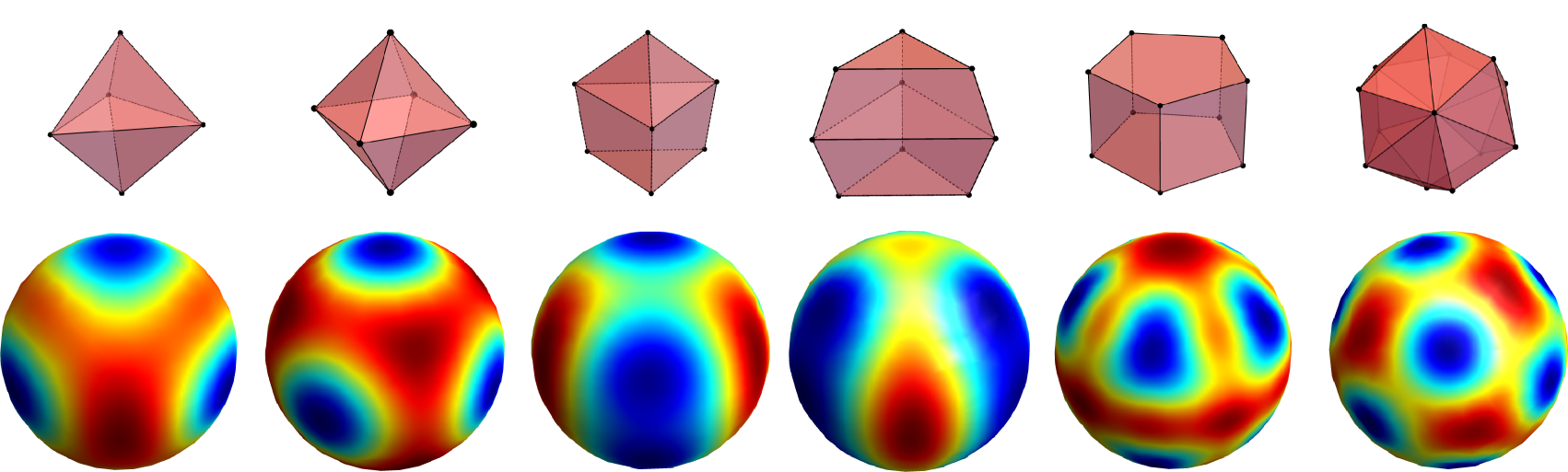
Figure 1: (Color online) Density plots of the SU(2) $Q$ functions for the optimal states in Table I for the cases $S=5/2,3,7/2,9/2,5$, and $7$ (from left to right, blue indicates the zero values and red maximal ones). On top, we sketch the Majorana constellation for each of them.

Table 1 lists the resulting states (which, in some cases, are not unique) for different selected values of $S$ . We also indicate the associated Majorana constellations. For completeness, in Fig. 1 we also plot the constellations as well as the $Q$-functions for some of these states.

Intuitively, one would expect that these constellations should have the points as symmetrically placed on the unit sphere as possible. This fits well with the notion of states of maximal Wehrl-Lieb entropy Baecklund and Bengtsson (2014). In more precise mathematical terms, such points may be generated via optimization with respect to a suitable criterion Saff and Kuijlaars (1997). Here, we explore the connection with spherical $t$-designs Delsarte et al. (1977), which are patterns of $N$ points on a sphere such that every polynomial of degree at most $t$ has the same average over the $N$ points as over the sphere. Thus, the $N$ points mimic a flat distribution up to order $t$, which obviously implies a fairly symmetric distribution.

For a given $S$, the maximal order of $M$ for which we can cancel out $\mathcal{A}_{M}^{(S)}$ does not follow a clear pattern. The numerical evidence suggests that $M_{\mathrm{max}}$ coincides with $t_{\mathrm{max}}$ in the corresponding spherical design, but further work is needed to support this conjecture.

Table 1: States that kill $\mathcal{A}_{M}^{(S)}$ for the indicated values of $S$. In the second column, we indicate the order $M$, which we conjecture is the highest possible. We give the nonzero state components $\Psi_{m}$ ($m=-S,\ldots,S$) and the Majorana constellation. We include the associated spherical $t$-design (with the maximal $t$ value) and the Queens of quantumness (with their unpolarization degree). “same” “similar” and “different” always refer to the closest description column to the left.

$S$	$M$	State	Constellation	Design	$t$	Queens	$M$
1	1	$\Psi_{0}=1$	radial line	same	1	same	1
$\frac{3}{2}$	1	$\Psi_{-\scriptsize{\frac{3}{2}}}=\Psi_{\scriptsize{\frac{3}{2}}}=\scriptsize{\frac{1}{\sqrt{2}}}$	equatorial triangle	same	1	same	1
2	2	$\Psi_{-1}=\scriptsize{\frac{1}{\sqrt{3}}},\quad\Psi_{2}=\scriptsize{\sqrt{\frac{2}{3}}}$	tetrahedron	same	2	same	2
$\frac{5}{2}$	1	$\Psi_{-\scriptsize{\frac{5}{2}}}=\Psi_{\scriptsize{\frac{5}{2}}}=\scriptsize{\frac{1}{\sqrt{2}}}$	equatorial triangle + poles	same	1	same	1
3	3	$\Psi_{-2}=\Psi_{2}=\scriptsize{\frac{1}{\sqrt{2}}}$	octahedron	same	3	same	3
$\frac{7}{2}$	2	$\Psi_{-\scriptsize{\frac{5}{2}}}=\Psi_{\scriptsize{\frac{1}{2}}}=\scriptsize{\sqrt{\frac{7}{18}}},\quad\Psi_{\scriptsize{\frac{7}{2}}}=\scriptsize{\sqrt{\frac{2}{9}}}$	two triangles + pole	similar	2	equatorial pentagon + poles	1
4	3	$\Psi_{-4}=\Psi_{4}=\scriptsize{\sqrt{\frac{5}{24}}},\quad\Psi_{0}=\scriptsize{\sqrt{\frac{7}{12}}}$	cube	same	3	see Giraud et al. (2010)	1
$\frac{9}{2}$	2	$\Psi_{-\scriptsize{\frac{9}{2}}}=\Psi_{\scriptsize{\frac{9}{2}}}=\scriptsize{\frac{1}{\sqrt{6}}},\quad\Psi_{-\scriptsize{\frac{3}{2}}}=\Psi_{\scriptsize{\frac{3}{2}}}=\scriptsize{\frac{1}{\sqrt{3}}}$	three triangles	similar	2	similar	1
5	3	$\Psi_{-5}=\Psi_{5}=\scriptsize{\frac{1}{\sqrt{3}}},\quad\Psi_{0}=\scriptsize{\frac{1}{\sqrt{5}}}$	pentagonal prism	similar	3	two staggered squares + poles	1
$\frac{11}{2}$	3	$\Psi_{-\scriptsize{\frac{11}{2}}}=\Psi_{\scriptsize{\frac{11}{2}}}=\scriptsize{\frac{\sqrt{17}}{12}},\quad\Psi_{-\scriptsize{\frac{5}{2}}}=\Psi_{\scriptsize{\frac{5}{2}}}=i\scriptsize{\frac{\sqrt{55}}{12}}$	pentagon + two triangles	similar	3	similar	1
6	5	$\Psi_{-5}=-\Psi_{5}=\scriptsize{\frac{\sqrt{7}}{5}},\quad\Psi_{0}=-\scriptsize{\frac{\sqrt{11}}{5}}$	icosahedron	same	5	same	5
7	4	$\Psi_{-6}=\Psi_{6}=\scriptsize{\sqrt{\frac{854}{3645}}},\quad\Psi_{-3}=\Psi_{3}=\scriptsize{\sqrt{\frac{637}{13420}}+i\sqrt{\frac{512603}{9783180}}}$	three squares + poles	different	4	—	–
		$\Psi_{0}=\scriptsize{\sqrt{\frac{12561757}{163053000}}}-\scriptsize{i\sqrt{\frac{512603}{2013000}}}$
10	5	$\Psi_{-10}=\Psi_{10}=\scriptsize{\sqrt{\frac{187}{1875}}},\quad\Psi_{-5}=-\Psi_{5}=\scriptsize{\sqrt{\frac{209}{625}}},\quad\Psi_{0}=\scriptsize{\sqrt{\frac{247}{1875}}}$	deformed dodecahedron	similar	5	—	–

The simplest nontrivial example are two-photon states, $S=1$. We find only first-order unpolarized states: these are biphotons generated in spontaneous parametric down-conversion, which were the first known to have hidden polarization Klyshko (1997).

With three photons, $S=3/2$, we have again only first-order unpolarized states: the constellation is an equilateral triangle inscribed in a great circle, which can be taken as the equator. This coincides with the three-point spherical 1-design.

For $S=2$, the Majorana constellation is a regular tetrahedron: it is the least-excited second-order unpolarized state. It is not surprising that the tetrahedron is the $2$-design with the lowest number of points.

The case $S=5/2$ does not admit a high degree of spherical symmetry: only first-order unpolarized states exist. There are neither five-photon $M=2$ unpolarized states Kolenderski and Demkowicz-Dobrzanski (2008); Crann et al. (2010) nor five-point $2$-designs Mimura (1990).

When increasing the number of photons to six, $S=3$, another Platonic solid appears: the regular octahedron. Now, we have the least-excited third-order unpolarized states, which, in addition, take on the maximum sum of the Stokes variances.

For $S=7/2$, an $M=2$ constellation consists of the north pole, an equilateral triangle inscribed at the $z=0.2424$ plane, and another equilateral triangle, with the same orientation (e.g., one vertex on the $x$-axis) at the $z=-0.5816$ plane. The spherical $t$-design has a larger separation between the triangles; but the corresponding Stokes vector does not vanish, so the $t$-design does not coincide with any unpolarized state.

The next Platonic solid, the cube, appears when $S=4$. The state is third-order unpolarized and its Majorana constellation coincides with the eight-point spherical $3$-design, which is the tightest for this number of points.

A nine-photon second-order unpolarized state, $S=9/2$, is generated by three equilateral triangles with the same orientation inscribed in the equator and in two symmetric rings. The highest nine-point spherical $t$-design has $t=2$ and a similar, but not identical, configuration because the two smaller triangles are displaced by a larger distance from the equator than the previous constellation. As a consequence, the nine-point spherical $2$-design is only first-order unpolarized.

The Majorana constellation for a maximally unpolarized 10-photon state ($S=5$) is similar to the matching spherical $t$-design and consists of two identical regular pentagons inscribed in rings symmetrically displaced from the equator. The maximally unpolarized state has the two pentagons a bit closer to the equator than the spherical $3$-design (that has $M=1$).

For larger photon numbers, the computational complexity of finding optimal designs becomes a real hurdle. The $t$-designs have been investigated in the range 2–100 and numerical evidence suggests that the optimal designs (in some instances, they are not unique) have been found . However, for some dimensions, e.g., 12 ($S=6$) and 20 ($S=10$), one would naïvely guess that the optimal designs fit with the icosahedron and the dodecahedron. For $S=6$ this turns out to be a correct guess, the corresponding state is unpolarized to the same order as the spherical $5$-design formed by the icosahedron. For $S=10$ this intuition fails: the optimal $t$-design is indeed a dodecahedron, but this Majorana constellation is third-order unpolarized, whereas this is a spherical $5$-design. If the dodecahedron is stretched (i.e., the four pentagonal rings that define its vertices are displaced against the pole), one can find a 20-photon fifth-order unpolarized state.

To check the correspondence between unpolarized states and optimal $t$-designs we look at dimension 14, which is the smallest number of points for which a spherical $4$-design, but not a $5$-design, exists. This consists of four equilateral triangles that are pairwise similar in size, displaced from the equator by the same distance, and rotated an angle $\pm\alpha$ or $\pm\beta$ around their surface normal, plus the two poles. The $t$-design state is only first-order unpolarized, but if the spacing and triangle orientation is optimized, the design can be made third-order unpolarized. There is indeed a 14-photon state that is fourth-order unpolarized: its Majorana constellation is made of three quadrangles and the poles, but this is only a $1$-design.

To round up, it is worth commenting on the connections that our theory shares with two recently introduced notions: anticoherent states Zimba (2006) and queens of quantumness Giraud et al. (2010). For completeness, in Table 1 we have also listed the configurations and the degree of unpolarization for these queens. Anticoherent states are in a sense “the opposite” of SU(2) coherent states: while the latter correspond as nearly as possible to a classical spin vector pointing in a given direction, the former “point nowhere”, i.e., the average Stokes vector vanishes and the fluctuations up to order $M$ are isotropic. The queens of quantumness are the most distant states (in the sense of a Hilbert-Schmidt distance) to the classical ones (states than can be written as a convex sum of projectors onto coherent states). In particular low-dimensional cases, these two instances coincide with our optimal states. However, we stress that our theory is built from first principles, starting from magnitudes that are routinely determined in the lab. Besides, we have an algebraic criterion, namely, the vanishing of the cumulative multipole distribution, that can be handled in a clear and compact manner.

When we interpret our $(2S+1)$-dimensional subspace as the symmetric subspace of a system of $S$ qubits, the kings appear also closely linked to other intriguing problems, such as maximally entangled symmetric states Aulbach et al. (2010); Giraud et al. (2015) and $k$-maximally mixed states Arnaud and Cerf (2013); Goyeneche and Życzkowski (2014).

Applications.— The main goal of quantum metrology is to measure a physical magnitude with surprising precision by exploiting quantum resources. In particular, tailoring polarization states to better detect SU(2) rotations is quite a relevant problem with direct applications to magnetometry, polarimetry, and metrology, in general Rozema et al. (2014).

In this respect, $N00N$ states [defined as $|N00N\rangle=(|S,S\rangle-|S,-S\rangle)/\sqrt{2}$] are known to be maximally sensitive to small phase shifts (i.e., to small rotations about the $S_{z}$-axis) for a fixed excitation $S$ Bollinger et al. (1996). This can be easily understood by looking at their Majorana constellation, which consists in just $2S$ equidistantly placed points around the Poincaré sphere equator. Since a rotation around the $S_{z}$ axis is described by the unitary operator $\hat{U}(\vartheta)=\exp(-i\vartheta\hat{S}_{z}/2)$, the states $|\mathrm{N00N}\rangle$ and $\hat{U}(\vartheta)|\mathrm{N00N}\rangle$ are orthogonal for $\pi/(2S)$. However, to make optimal use of a $N00N$ state it is essential to know the rotation axis so as to ensure that the state is aligned with the axis to achieve its best sensitivity: the rotation resolution is thus highly directional for a $N00N$ state.

This is precisely the advantage of maximally unpolarized states: having a high degree of spherical symmetry, they resolve rotations around any axis approximately equally well. This has been confirmed for the Platonic solids Kolenderski and Demkowicz-Dobrzanski (2008): Platonic states saturate the optimal average sensitivity to rotations about any axis; $N00N$ states outperform these states about one specific axis Rozema (2014). Indeed, for the Platonic solids, rotations around all the facets normal axes map the Majorana constellation onto itself for rotations of $2\pi/3$ (tetrahedron, octahedron and icosahedron), $\pi/2$ (cube), or $2\pi/5$ (dodecahedron). It is clear that for other constellations and other rotation axes the Majorana constellation will only become approximately identical, but the statement is more likely to hold true.

In a different vein, we draw attention to the structural similarity between the kings of quantumness and quantum error correcting codes: in both cases, low-order terms in the expansion of the density matrices are required to vanish.

As a final but relevant remark, we stress that all the basic tools needed for our treatment (Schwinger representation, multipole expansion and constellations) have been extended in a direct way to other symmetries, such as SU(3) Bányai et al. (1966) or Heisenberg-Weyl Ivan et al. (2012). Therefore, the notion of kings of quantumness can be easily developed for other systems. Work along these lines is already in progress in our group.

Concluding remarks.— In short, we have consistently reaped the benefits of the cumulative distribution of polarization multipoles, which is a sensible and experimentally realizable quantity. We have proven that SU(2) coherent states maximize that quantity to all orders: in this way, they manifest their classical virtues. Their opposite counterparts, minimizing that quantity, are certainly the kings of quantumness

Apart from their indisputable geometrical beauty, there surely is plenty of room for the application of these states, whose generation has started to be seriously considered in several groups.

The authors acknowledge interesting discussions with Prof. Daniel Braun and Olivia di Matteo. Financial support from the Swedish Research Council (VR) through its Linnaeus Center of Excellence ADOPT and Contract No. 621-2011-4575, the CONACyT (Grant 106525), the European Union FP7 (Grant Q-ESSENCE), and the Program UCM-Banco Santander (Grant GR3/14) is gratefully acknowledged. GB thanks the MPL for hosting him and the Wenner-Gren Foundation for economic support.

Appendix: Optimal states.— We have to maximize the cumulative multipole distribution (4) for a pure state $|\Psi\rangle=\sum_{m=-S}^{S}\Psi_{m}\,|S,m\rangle$, which takes the form (5). If we use integral representation for the product of two Clebsch-Gordan coefficients Varshalovich et al. (1988), we get

$$\mathcal{A}_{K}^{(S)}=\sum_{m,m^{\prime}=-S}^{S}\sum_{n,n^{\prime}=-S}^{S}\frac{2S+1}{8\pi^{2}}\sum_{K=0}^{M}\sum_{q=-K}^{K}\frac{2K+1}{2S+1}\Psi_{m^{\prime}}\Psi_{m}^{\ast}\Psi_{n}\Psi_{n^{\prime}}^{\ast}$$

$$\times\int dR\,D_{mn}^{S}(R)\,D_{m^{\prime}n^{\prime}}^{S\ast}(R)\,D_{qq}^{K}(R)\,,$$ (8)

where $D_{mn}^{S}$ are the Wigner $D$-functions and $R$ refers to the three Euler angles $(\alpha,\beta,\gamma)$ and the integration is on the group manifold

$$\int dR\ f(R)\equiv\int_{0}^{2\pi}d\alpha\int_{0}^{\pi}d\beta\sin\beta\int_{0}^{2\pi}d\gamma f(\alpha,\beta,\gamma)\ .$$ (9)

Since

$$\sum_{q=-K}^{K}D_{qq}^{K}(R)=\chi_{K}(\omega),$$ (10)

where $\chi_{K}(\omega)$ is a SU(2) generalized character and $\cos(\omega/2)=\cos(\beta/2)\cos[(\alpha+\gamma)/2]$, we rewrite $\mathcal{A}_{M}^{(S)}$ as

$$\mathcal{A}_{M}^{(S)}=\sum_{K=0}^{M}\frac{2K+1}{8\pi^{2}}\int dR\,\chi_{K}(\omega)\mid\langle\Psi|\hat{T}_{g}^{S}|\Psi\rangle\mid^{2}.$$ (11)

and $\hat{T}_{g}$ is the group action. Then, we observe that the above is

$$\mathcal{A}_{M}^{(S)}=\mathop{\mathrm{Tr}}\nolimits\Big{[}|\Psi\rangle\langle\Psi|\otimes|\tilde{\Psi}\rangle\langle\tilde{\Psi}|$$

$$\times\sum_{K=0}^{M}\frac{2K+1}{8\pi^{2}}\int dR\,\chi_{K}(\omega)\hat{T}_{g}^{S}\otimes\hat{T}_{g}^{S}\Big{]},$$ (12)

with

$$|\tilde{\Psi}\rangle=\sum_{m=-S}^{S}(-1)^{m}\,\Psi_{-m}^{\ast}\,|S,m\rangle.$$ (13)

Because the integral

$$\frac{1}{4\pi^{2}}\int dR\,\chi_{K}(\omega)\hat{T}_{g}^{S}\otimes\hat{T}_{g}^{S\dagger}=c_{K}\Pi_{K},$$ (14)

where $\Pi_{K}$ is the identity on the $(2K+1)$-dimensional irreducible SU(2) subspace which appear in the tensor product of $\mathcal{H}_{S}\otimes\mathcal{H}_{S}$ [i.e., $\mathop{\mathrm{Tr}}\nolimits(\Pi_{K})=2K+1$], then

$$\mathcal{A}_{M}^{(S)}=\sum_{K=1}^{M}\langle\tilde{\Psi}|\langle\Psi|\Pi_{K}|\Psi\rangle|\tilde{\Psi}\rangle.$$ (15)

Such overlap is maximized (all coefficients are the same) whenever in every subspace of dim $2K+1$ there is only one element from the decomposition $|\Psi\rangle|\tilde{\Psi}\rangle$, which is consistent with (13). The only states that at decomposition on representations produce a single state in each invariant subspace are the basis states $|S,m\rangle$, so that $|\tilde{\Psi}\rangle=(-1)^{m}\,|S,-m\rangle$, then

$$\mathcal{A}_{M}^{(S)}=\sum_{K=1}^{M}\frac{2K+1}{2S+1}\left|C_{SS,K0}^{S-S}\right|^{2}\,.$$ (16)

Since the maximum value of $C_{Sm_{,}S-m}^{K0}$ is $C_{SS,S-S}^{K0}$, the states $|S,\pm S\rangle$ maximize $\mathcal{A}_{M}^{(S)}$, as heralded before.

References

- Klimov et al. (2005) A. B. Klimov, L. L. Sánchez-Soto, E. C. Yustas, J. Söderholm, and G. Björk, “Distance-based degrees of polarization for a quantum field,” Phys. Rev. A 72, 033813 (2005).
- Sehat et al. (2005) A. Sehat, J. Söderholm, G. Björk, P. Espinoza, A. B. Klimov, and L. L. Sánchez-Soto, “Quantum polarization properties of two-mode energy eigenstates,” Phys. Rev. A 71, 033818 (2005).
- Marquardt et al. (2007) Ch. Marquardt, J. Heersink, R. Dong, M. V. Chekhova, A. B. Klimov, L. L. Sánchez-Soto, U. L. Andersen, and G. Leuchs, “Quantum reconstruction of an intense polarization squeezed optical state,” Phys. Rev. Lett. 99, 220401 (2007).
- Klimov et al. (2010) A. B. Klimov, G. Björk, J. Söderholm, L. S. Madsen, M. Lassen, U. L. Andersen, J. Heersink, R. Dong, Ch. Marquardt, G. Leuchs, and L. L. Sánchez-Soto, “Assessing the polarization of a quantum field from Stokes fluctuations,” Phys. Rev. Lett. 105, 153602 (2010).
- Müller et al. (2012) C. R. Müller, B. Stoklasa, C. Peuntinger, C. Gabriel, J. Řeháček, Z. Hradil, A. B. Klimov, G. Leuchs, Ch. Marquardt, and L. L. Sánchez-Soto, “Quantum polarization tomography of bright squeezed light,” New J. Phys. 14, 085002 (2012).
- Björk et al. (2012) G. Björk, J. Söderholm, Y. S. Kim, Y. S. Ra, H. T. Lim, C. Kothe, Y. H. Kim, L. L. Sánchez-Soto, and A. B. Klimov, “Central-moment description of polarization for quantum states of light,” Phys. Rev. A 85, 053835 (2012).
- Singh and Prakash (2013) R. S. Singh and H. Prakash, “Degree of polarization in quantum optics through the second generalization of intensity,” Phys. Rev. A 87, 025802 (2013).
- Sánchez-Soto et al. (2013) L. L. Sánchez-Soto, A. B. Klimov, P. de la Hoz, and G. Leuchs, “Quantum versus classical polarization states: when multipoles count,” J. Phys. B 46, 104011 (2013).
- de la Hoz et al. (2013) P. de la Hoz, A. B. Klimov, G. Björk, Y. H. Kim, C. Müller, Ch. Marquardt, G. Leuchs, and L. L. Sánchez-Soto, “Multipolar hierarchy of efficient quantum polarization measures,” Phys. Rev. A 88, 063803 (2013).
- de la Hoz et al. (2014) P. de la Hoz, G. Björk, A. B. Klimov, G. Leuchs, and L. L. Sánchez-Soto, “Unpolarized states and hidden polarization,” Phys. Rev. A 90, 043826 (2014).
- Majorana (1932) E. Majorana, “Atomi orientati in campo magnetico variabile,” Nuovo Cimento 9, 43–50 (1932).
- Conway et al. (1996) John H. Conway, Ronald H. Hardin, and Neil J. A. Sloane, “Packing lines, planes, etc.: Packings in Grassmannian spaces,” Exp. Math. 5, 139–159 (1996).
- Saff and Kuijlaars (1997) E. B. Saff and A. B. J. Kuijlaars, “Distributing many points on a sphere,” Math. Intell. 19, 5–11 (1997).
- Luis and Sánchez-Soto (2000) A. Luis and L. L. Sánchez-Soto, “Quantum phase difference, phase measurements and Stokes operators,” Prog. Opt. 41, 421–481 (2000).
- Born and Wolf (1999) M. Born and E. Wolf, Principles of Optics, 7th ed. (Cambridge University Press, Cambridge, 1999).
- Chaturvedi et al. (2006) S. Chaturvedi, G. Marmo, and N. Mukunda, “The Schwinger representation of a group: concept and applications,” Rev. Math. Phys. 18, 887–912 (2006).
- Varshalovich et al. (1988) D. A. Varshalovich, A. N. Moskalev, and V. K. Khersonskii, Quantum Theory of Angular Momentum (World Scientific, Singapore, 1988).
- Raymer et al. (2000) M. G. Raymer, D. F. McAlister, and A. Funk, “Measuring the quantum polarization state of light,” in Quantum Communication, Computing, and Measurement 2, edited by P. Kumar (Plenum, New York, 2000).
- Karassiov and Masalov (2004) V. P. Karassiov and A. V. Masalov, “The method of polarization tomography of radiation in quantum optics,” JETP 99, 51–60 (2004).
- Fano and Racah (1959) U. Fano and G. Racah, Irreducible Tensorial Sets (Academic Press, New York, 1959)).
- Blum (1981) K. Blum, Density Matrix Theory and Applications (Plenum, New York, 1981).
- Perelomov (1986) A. Perelomov, Generalized Coherent States and their Applications (Springer, Berlin, 1986).
- Prakash and Chandra (1971) H. Prakash and N. Chandra, “Density operator of unpolarized radiation,” Phys. Rev. A 4, 796–799 (1971).
- Agarwal (1971) G. S. Agarwal, “On the state of unpolarized radiation,” Lett. Nuovo Cimento 1, 53–56 (1971).
- Bosma et al. (1997) W. Bosma, J. Cannon, and C. Playoust, “The Magma algebra system. i. the user language,” J. Symbolic Comput. 24, 235–265 (1997).
- Note (1) A more detailed list of minimal states can be found in http://polarization.markus-grassl.de.
- Baecklund and Bengtsson (2014) A. Baecklund and I. Bengtsson, “Four remarks on spin coherent states,” Phys. Scr. T163, 014012 (2014).
- Delsarte et al. (1977) P. Delsarte, J. M. Goethals, and J. J. Seidel, “Spherical codes and designs,” Geom. Dedicata 6, 363–388 (1977).
- Giraud et al. (2010) O. Giraud, P. Braun, and D. Braun, “Quantifying quantumness and the quest for queens of quantumness,” New J. Phys. 12, 063005 (2010).
- Klyshko (1997) D. M. Klyshko, “Polarization of light: fourth-order effects and polarization-squeezed states,” JETP 84, 1065–1079 (1997).
- Kolenderski and Demkowicz-Dobrzanski (2008) P. Kolenderski and R. Demkowicz-Dobrzanski, “Optimal state for keeping reference frames aligned and the platonic solids,” Phys. Rev. A 78, 052333 (2008).
- Crann et al. (2010) J. Crann, R. Pereira, and D. W. Kribs, “Spherical designs and anticoherent spin states,” J. Phys. A 43, 255307 (2010).
- Mimura (1990) Y. Mimura, “A construction of spherical -design,” Graphs Combinator. 6, 369–372 (1990).
- Note (2) For a complete account see http://neilsloane.com/sphdesigns/.
- Zimba (2006) J. Zimba, ““Anticoherent” spin states via the Majorana representation,” EJTP 3, 143–156 (2006).
- Aulbach et al. (2010) M. Aulbach, D. Markham, and M. Murao, “The maximally entangled symmetric state in terms of the geometric measure,” New J. Phys 12, 073025 (2010).
- Giraud et al. (2015) O. Giraud, D. Braun, D. Baguette, T. Bastin, and J. Martin, “Tensor representation of spin states,” Phys. Rev. Lett. 114, 080401 (2015).
- Arnaud and Cerf (2013) L. Arnaud and N. J. Cerf, “Exploring pure quantum states with maximally mixed reductions,” Phys. Rev. A 87, 012319 (2013).
- Goyeneche and Życzkowski (2014) D. Goyeneche and K. Życzkowski, “Genuinely multipartite entangled states and orthogonal arrays,” Phys. Rev. A 90, 022316 (2014).
- Rozema et al. (2014) L. A. Rozema, D. H. Mahler, R. Blume-Kohout, and A. M. Steinberg, “Optimizing the choice of spin-squeezed states for detecting and characterizing quantum processes,” Phys. Rev. X 4, 041025 (2014).
- Bollinger et al. (1996) J. J. Bollinger, Wayne M. Itano, D. J. Wineland, and D. J. Heinzen, “Optimal frequency measurements with maximally correlated states,” Phys. Rev. A 54, R4649–R4652 (1996).
- Rozema (2014) L. A. Rozema, Experimental quantum measurement with a few photons, Ph.D. thesis, University of Toronto (2014).
- Bányai et al. (1966) L. Bányai, N. Marinescu, I. Raszillier, and V. Rittenberg, “Irreducible tensors for the group su(3),” Commun. Math. Phys. 2, 121–132 (1966).
- Ivan et al. (2012) J. S. Ivan, N. Mukunda, and R. Simon, “Moments of non-Gaussian Wigner distributions and a generalized uncertainty principle: I. the single-mode case,” J. Phys. A: Math. Theor. 45, 195305 (2012).