Possibility of higher dimensional anisotropic compact star

Abstract

We provide here a new class of interior solutions for anisotropic stars admitting conformal motion in higher dimensional noncommutative spacetime. The Einstein field equations are solved by choosing a particular density distribution function of Lorentzian type as provided by Nazari and Mehdipour Nozari2009 ; Mehdipour2012 under noncommutative geometry. Several cases with dimensions $4D$ and higher, e.g. $5D$, $6D$ and $11D$ have been discussed separately ($D$ stands for dimension of the spacetime). An overall observation is that the model parameters, such as density, radial pressure, transverse pressure and anisotropy all are well behaved and represent a compact star with mass $2.27$ $M_{\odot}$ and radius $4.17$ km. However, emphasis has been given on the acceptability of the model from a physical point of view. As a consequence it is observed that higher dimensions, i.e. beyond $4D$ spacetime, exhibit several interesting yet bizarre features which are not at all untenable for a compact stellar model of strange quark type and thus dictates a possibility of its extra dimensional existence.

1 Introduction

To model a compact object it is generally assumed that the underlying matter distribution is homogeneous i.e. perfect fluid obeying Tolman-Oppenheimer-Volkoff (TOV) equation. The nuclear matter of density $\rho\sim 10^{15}$ gm/cc, which is expected at the core of the compact terrestrial object, becomes anisotropic in nature as was first argued by Ruderman Ruderman1972 . In case of anisotropy the pressure inside the fluid sphere can specifically be decomposed into two parts: radial pressure, $p_{r}$ and the transverse pressure, $p_{t}$, where $p_{t}$ is in the perpendicular direction to $p_{r}$. Their difference $\Delta=p_{t}-p_{r}$ is defined as the anisotropic factor. Now, the anisotropic force ($\frac{2\Delta}{r}$) will be repulsive in nature if $\Delta>0$ or equivalently $p_{t}>p_{r}$ and attractive if $p_{t}<p_{r}$. So it is reasonable to consider pressure anisotropy to develop our model under investigation. It has been shown that in case of anisotropic fluid the existence of repulsive force helps to construct compact objects gokhroo1994 .

Anisotropy may occur for different reasons in any stellar distribution. It could be introduced by the existence of the solid core or for the presence of type $3A$ superfluid Kippenhahn1990 . Different kinds of phase transitions sokolov1980 , pion condensation  sawyer1972 etc. are also reasonable for anisotropy. It may also occur by the effects of slow rotation in a star. Bowers and Liang Bowers1974 showed that anisotropy might have non-negligible effects on such parameters like equilibrium mass and surface redshift. Very recently other theoretical advances also indicate that the pressure inside a compact object is not essentially isotropic in nature Varela2010 ; Rahaman2010a ; Rahaman ; Rahaman2012a ; Kalam2012 ; Hossein2012 ; Kalam2013 .

In recent years the extension of General Relativity to higher dimensions has become a topic of great interest. As a special mention in this line of thinking we note that ‘Whether the usual solar system tests are compatible with the existence of higher spatial dimensions’ has been investigated by Rahaman et al. Rahaman2 . Some other studies in higher dimension are done by Liu and Overduin Liu for the motion of test particle whereas Rahaman et al. Rahaman3 have investigated higher dimensional gravastars.

One of the most interesting outcomes of string theory is that the target spacetime coordinates become noncommuting operators on $D$-brane Witten1996 ; Seiberg1999 . Now the noncommutativity of a spacetime can be encoded in the commutator $\left[x^{\mu},x^{\nu}\right]=i\theta^{\mu\nu}$, where $\theta^{\mu\nu}$ is an anti-symmetric matrix and is of dimension $(length)^{2}$ which determines the fundamental cell discretization of spacetime. It is similar to the way the Planck constant $\hbar$ discretizes phase space Smailagic2003 .

In the literature many studies are available on noncommutative geometry, for example, Nazari and Mehdipour Nozari2009 used Lorentzian distribution to analyze ‘Parikh-Wilczek Tunneling’ from noncommutative higher dimensional black holes. Besides this investigation some other noteworthy works are on galactic rotation curves inspired by a noncommutative-geometry background Rahaman2012b , stability of a particular class of thin-shell wormholes in noncommutative geometry Peter2012 , higher-dimensional wormholes with noncommutative geometry Rahaman2012c , noncommutative BTZ black hole Rahaman2013 , noncommutative wormholes Rahaman2014a and noncommutative wormholes in $f(R)$ gravity with Lorentzian distribution Rahaman2014b .

It is familiar to search for the natural relationship between geometry and matter through the Einstein field equations where it is very convenient to use inheritance symmetry. The well known inheritance symmetry is the symmetry under conformal Killing vectors (CKV) i.e.

$$L_{\xi}g_{ik}=\psi g_{ik},$$ (1)

where $L$ is the Lie derivative of the metric tensor, which describes the interior gravitational field of a stellar configuration with respect to the vector field $\xi$, and $\psi$ is the conformal factor. It is supposed that the vector $\xi$ generates the conformal symmetry and the metric $g$ is conformally mapped onto itself along $\xi$. It is to note that neither $\xi$ nor $\psi$ need to be static even though one considers a static metric Harko1 ; Harko2 . We also note that (i) if $\psi=0$ then Eq. (1) gives the Killing vector, (ii) if $\psi=$ constant it gives homothetic vector and (iii) if $\psi=\psi(\textbf{x},t)$ then it yields conformal vectors. Moreover it is to be mentioned that for $\psi=0$ the underlying spacetime becomes asymptotically flat which further implies that the Weyl tensor will also vanish. So CKV provides a deeper insight of the underlying spacetime geometry.

A large number of works on conformal motion have been done by several authors. A class of solutions for anisotropic stars admitting conformal motion have been studied by Rahaman et al. Rahaman7 . In a very recent work Rahaman et al. Rahaman8 have also described conformal motion in higher dimensional spacetimes. Charged gravastar admitting conformal motion has been studied by Usmani et al. Usmani2011 . Contrary to this work Bhar piyali has studied higher dimensional charged gravastar admitting conformal motion whereas relativistic stars admitting conformal motion has been analyzed by Rahaman et al. Rahaman2010b . Inspired by these earlier works on conformal motion we are looking forward for a new class of solutions of anisotropic stars under the framework of General Relativity inspired by noncommutative geometry in four and higher dimensional spacetimes.

In the presence of noncommutative geometry there are two different distributions available in the literature: (a) Gaussian and (b) Lorentzian Mehdipour2012 . Though these two mass distributions represent similar quantitative aspects, for the present investigation we are exploiting a particular Lorentzian-type energy density of the static spherically symmetric smeared and particle-like gravitational source in the multi-dimensional general form Nozari2009 ; Mehdipour2012

$$\rho=\frac{M\sqrt{\phi}}{\pi^{2}(r^{2}+\phi)^{\frac{n+2}{2}}},$$ (2)

where $M$ is the total smeared mass of the source, $\phi$ is the noncommutative parameter which bears a minimal width $\sqrt{\phi}$ and $n$ is positive integer greater than 1. In this approach, generally known as the noncommutative geometry inspired model, via a minimal length caused by averaging noncommutative coordinate fluctuations cures the curvature singularity in black holes Smailagic2003 ; Spallucci2006 ; Banerjee2009 ; Modesto2010 ; Nicolini2011 . It has been argued that it is not required to consider the length scale of the coordinate noncommutativity to be the same as the Planck length as the noncommutativity influences appears on a length scale which can behave as an adjustable parameter corresponding to that pertinent scale Mehdipour2012 .

It is interesting to note that Rahaman et al. Rahaman7 have found out a new class of interior solutions for anisotropic compact stars admitting conformal motion under $4D$ framework of GR. On the other hand, Rahaman et al. Rahaman8 have studied different dimensional fluids, higher as well as lower, inspired by noncommutative geometry with Gaussian distribution of energy density and have shown that at $4D$ only one can get a stable configuration for any spherically symmetric stellar system. However, in the present work we have extended the work of Rahaman et al. Rahaman7 to higher dimensions and that of Rahaman et al. Rahaman8 to higher dimensions with energy density in the form of Lorentzian distribution. In this approach we are able to generalize both the above mentioned works to show that compacts stars may exist even in higher dimensions.

In this paper, therefore we use noncommutative geometry inspired model to combine the microscopic structure of spacetime with the relativistic description of gravity. The plan of the present investigation is as follows: in Section 2 we formulate the Einstein field equations for the interior spacetime of the anisotropic star. In Section 3 we solve the Einstein field Equations by using the density function of Lorentzian distribution type in higher dimensional spacetime as given by Nozari and Mehdipour Nozari2009 . We consider the cases $n=~{}2,~{}3,~{}4$ and $9$ i.e. $4D,~{}5D,~{}6D$ and $11D$ spacetimes in Section 4 to examine expressions for physical parameters whereas the matching conditions are provided in Section 5. Various physical properties are explored in Section 6 with interesting features of the model and present them with graphical plots for comparative studies among the results of different dimensional spacetimes. Finally we complete the paper with some concluding remarks in Section 7.

2 The interior spacetime and the Einstein field equations

To describe the static spherically symmetric spacetime (in geometrical units $G=1=c$ here and onwards) in higher dimension the line element can be given in the standard form

$$ds^{2}=-e^{\nu(r)}dt^{2}+e^{\lambda(r)}dr^{2}+r^{2}d\Omega_{n}^{2},$$ (3)

where

$$d\Omega_{n}^{2}=d\theta_{1}^{2}+\sin^{2}\theta_{1}d\theta_{2}^{2}+\sin^{2}\theta_{1}\sin^{2}\theta_{2}d\theta_{3}^{2}+...+\prod_{j=1}^{n-1}\sin^{2}\theta_{j}d\theta_{n}^{2},$$ (4)

where $\lambda$, $\nu$ are functions of the radial coordinate $r$. Here we have used the notation $D=n+2$, $D$ is the dimension of the spacetime.

The energy momentum tensor for the matter distribution can be taken in its usual form Lobo

$$T_{\nu}^{\mu}=(\rho+p_{r})u^{\mu}u_{\nu}-p_{r}g^{\mu}_{\nu}+(p_{t}-p_{r})\eta^{\mu}\eta_{\nu},$$ (5)

with $u^{\mu}u_{\mu}=-\eta^{\mu}\eta_{\mu}=1$ and $u^{\mu}\eta_{\nu}=0$. Here the vector $u^{\mu}$ is the fluid $(n+2)$-velocity and $\eta^{\mu}$ is the unit space-like vector which is orthogonal to $u^{\mu}$, where $\rho$ is the matter density, $p_{r}$ is the radial pressure in the direction of $\eta^{\mu}$ and $p_{t}$ is the transverse pressure in the orthogonal direction to $p_{r}$. Since the pressure is anisotropic in nature so for our model $p_{r}\neq p_{t}$. Here $p_{t}-p_{r}=\Delta$ is the measure of anisotropy, as defined earlier.

Now for higher ( $n\geq 2)$ dimensional spacetime the Einstein equations can be written as Rahaman2012b

$$e^{-\lambda}\left[\frac{n\lambda^{\prime}}{2r}-\frac{n(n-1)}{2r^{2}}\right]+\frac{n(n-1)}{2r^{2}}=8\pi\rho=8\pi T_{0}^{0},$$ (6)

$$e^{-\lambda}\left[\frac{n(n-1)}{2r^{2}}+\frac{n\nu^{\prime}}{2r}\right]-\frac{n(n-1)}{2r^{2}}=8\pi p_{r}=-8\pi T_{1}^{1},$$ (7)

$$\frac{1}{2}e^{-\lambda}\left[\frac{1}{2}(\nu^{\prime})^{2}+\nu^{\prime\prime}-\frac{1}{2}\lambda^{\prime}\nu^{\prime}+\frac{(n-1)}{r}(\nu^{\prime}-\lambda^{\prime})+\frac{(n-1)(n-2)}{r^{2}}\right]$$

$$-\frac{(n-1)(n-2)}{2r^{2}}=8\pi p_{t}=-8\pi T_{2}^{2}=-8\pi T_{3}^{3},$$ (8)

where $\prime$ denotes differentiation with respect to the radial coordinate $r$ i.e. $\prime\equiv\frac{d}{dr}$.

3 The solution under conformal Killing vector

Mathematically, conformal motions or conformal Killing vectors (CKV) are motions along which the metric tensor of a spacetime remains invariant up to a scale factor. A conformal vector field can be defined as a global smooth vector field $x$ on a manifold, $\ss$, such that for the metric $g_{ab}$ in any coordinate system on $\ss$ $x_{a;b}=\psi g_{ab}+F_{ab}$, where $\psi:\ss\rightarrow real~{}number$ is the smooth conformal function of $x$, $F_{ab}$ is the conformal bivector of $x$. This is equivalent to $L_{x}g_{ik}=\psi g_{ik}$, (as considered in Eq. (1) in the usual form) where $L_{x}$ signifies the Lie derivatives along $x_{a}$.

To search the natural relation between geometry and matter through the Einstein equations, it is useful to use inheritance symmetry. The well known inheritance symmetry is the symmetry under conformal Killing vectors (CKV). These provide a deeper insight into the spacetime geometry. The CKV facilitate generation of exact solutions to the Einstein’s field equations. The study of conformal motions in spacetime is physically very important because it can lead to the discovery of conservation laws and devise spacetime classification schemes. Einstein’s field equations being highly non linear partial differential equations, one can reduce the partial differential equations to ordinary differential equations by use of CKV. It is still a challenging problem to the theoretical physicists to know the exact nature and characteristics of compact stars and elementary particle like electron.

Let us therefore assume that our static spherically symmetry spacetime admits an one parameter group of conformal motion. The conformal Killing vector, as given in Eq. (1), can be written in a more convenient form:

$$L_{\xi}g_{ik}=\xi_{i;k}+\xi_{k;i}=\psi g_{ik},$$ (9)

where both $i$ and $k$ take the values $~{}1,~{}2...,~{}n+2$. Here $\psi$ is an arbitrary function of the radial coordinate $r$ and $\xi$ is the orbit of the group. The metric $g_{ij}$ is conformally mapped onto itself along $\xi_{i}$.

Let us further assume that the orbit of the group to be orthogonal to the velocity vector field of the fluid,

$$\xi^{\mu}u_{\mu}=0.$$ (10)

As a consequence of the spherically symmetry from Eq. (10) we have

$$\xi^{1}=\xi^{3}=...=\xi^{n+1}=0.$$

Now the conformal Killing equation for the line element (3) gives the following equations:

$$\xi^{2}\nu^{\prime}=\psi,$$ (11)

$$\xi^{n+2}=C_{1},$$ (12)

$$\xi^{2}=\frac{\psi r}{2},$$ (13)

$$\xi^{2}\lambda^{\prime}+2{\xi^{2}}^{\prime}=\psi,$$ (14)

where $2$ stands for the spatial coordinates $r$,‘$\prime$’ and ‘,’ denotes the partial derivative with respect to $r$ and $C_{1}$ is a constant.

The above set of equations consequently gives

$$e^{\nu}=C_{2}^{2}r^{2},$$ (15)

$$e^{\lambda}=\left(\frac{C_{3}}{\psi}\right)^{2},$$ (16)

$$\xi^{i}=C_{1}\delta_{n+2}^{i}+\left(\frac{\psi r}{2}\right)\delta_{2}^{i},$$ (17)

where $\delta$ stands for the ‘Kronecker delta’ and $C_{2}$, $C_{3}$ are constants of integrations.

Using Eqs. (15)-(17) in the Einstein field Eqs. (6)-(8), we get

$$\frac{n(n-1)}{2r^{2}}\left(1-\frac{\psi^{2}}{C_{3}^{2}}\right)-\frac{n\psi\psi^{\prime}}{rC_{3}^{2}}=8\pi\rho,$$ (18)

$$\frac{n}{2r^{2}}\left[(n+1)\frac{\psi^{2}}{C_{3}^{2}}-(n-1)\right]=8\pi p_{r},$$ (19)

$$\frac{n\psi\psi^{\prime}}{rC_{3}^{2}}+n(n-1)\frac{\psi^{2}}{2r^{2}C_{3}^{2}}-\frac{(n-1)(n-2)}{2r^{2}}=8\pi p_{t}.$$ (20)

We thus have three independent Eqs. (18)-(20) with four unknowns $\rho$, $p_{r}$, $p_{t}$, $\psi$. So we are free to choose any physically reasonable ansatz for any one of these four unknowns. Hence we choose density profile $\rho$ in the form given in Eq. (2) in connection to higher dimensional static and spherically symmetric Lorentzian distribution of smeared matter as provided by Nozari and Mehdipour Nozari2009 . This density profile will be employed as a key tool in our present study.

Therefore, substituting Eq. (2) into (18) and solving, we obtain

$$\psi^{2}=C_{3}^{2}-\frac{16MC_{3}^{2}\sqrt{\phi}}{n\pi}\frac{1}{r^{n-1}}\int\frac{r^{n}}{(r^{2}+\phi)^{\frac{n+2}{2}}}dr+\frac{A}{r^{n-1}},$$ (21)

where $A$ is a constant of integration which is determined by invoking suitable boundary conditions.

Now the equation (21) gives the expression of the conformal factor $\psi$. Assigning $n=~{}2,~{}3,~{}4$ and $9$ i.e. $4D,~{}5D,~{}6D$ and $11D$ spacetimes respectively if we perform the above integral then the conformal factor $\psi$ can be obtained for different dimension that is necessary to find out the other physical parameter namely $p_{r}$ and $p_{t}$ for these dimension. Here $A,~{}-\infty<A<\infty$, is a constant of integration that can be later on found out from the boundary condition $p_{r}(R)=0$, $R$ being the radius of the star.

4 Exact solutions of the models in different dimensions

The above set of equations are associated with dimensional parameter $n$ and hence to get a clear picture of the physical system under different spacetimes we are interested for studying several cases starting from standard $4D$ to higher $5D$, $6D$ and $11D$ spacetimes as shown below.

4.1 Four dimensional spacetime ($n=2$)

The conformal parameter $\psi(r)$ and the metric potential $e^{\lambda}$ are given as,

$$\psi=\sqrt{C_{3}^{2}-\frac{4MC_{3}^{2}\sqrt{\phi}}{\pi r}\left[\frac{1}{\sqrt{\phi}}\arctan\left(\frac{r}{\sqrt{\phi}}\right)-\frac{r}{r^{2}+\phi}\right]+\frac{A}{r}},$$ (22)

$$e^{-\lambda}=1+\frac{A}{C_{3}^{2}r}-\frac{4M\sqrt{\phi}}{\pi r}\left[\frac{1}{\sqrt{\phi}}\arctan\left(\frac{r}{\sqrt{\phi}}\right)-\frac{r}{r^{2}+\phi}\right].$$ (23)

The radial and transverse pressures are obtained as

$$p_{r}=\frac{1}{8\pi r^{2}}\left[2+\frac{3A}{C_{3}^{2}r}-\frac{12M\sqrt{\phi}}{\pi r}\left\{\frac{1}{\sqrt{\phi}}\arctan\left(\frac{r}{\sqrt{\phi}}\right)-\frac{r}{r^{2}+\phi}\right\}\right],$$ (24)

$$p_{t}=\frac{1}{8\pi}\left[\frac{1}{r^{2}}-\frac{8M\sqrt{\phi}}{\pi(r^{2}+\phi)^{2}}\right].$$ (25)

To find the above constant of integration we impose the boundary condition $p_{r}(r=R)=0$, where $R$ is the radius of the fluid sphere as mentioned earlier, which gives

$$A=\frac{4MC_{3}^{2}\sqrt{\phi}}{\pi}\left\{\frac{1}{\sqrt{\phi}}\arctan\left(\frac{R}{\sqrt{\phi}}\right)-\frac{R}{R^{2}+\phi}\right\}-\frac{2}{3}C_{3}^{2}R.$$ (26)

4.2 Five dimensional spacetime ($n=3$)

In this case the solution set can be obtained as follows:

$$\psi=\sqrt{C_{3}^{2}+\frac{16MC_{3}^{3}\sqrt{\phi}}{9\pi r^{2}}\frac{3r^{2}+2\phi}{(r^{2}+\phi)^{\frac{3}{2}}}+\frac{A}{r^{2}}},$$ (27)

$$e^{-\lambda}=1+\frac{16M\sqrt{\phi}}{9\pi r^{2}}\frac{3r^{2}+2\phi}{(r^{2}+\phi)^{\frac{3}{2}}}+\frac{A}{C_{3}^{2}r^{2}},$$ (28)

$$p_{r}=\frac{3}{8\pi r^{2}}\left[1+\frac{32M\sqrt{\phi}}{9\pi r^{2}}\frac{3r^{2}+2\phi}{(r^{2}+\phi)^{\frac{3}{2}}}+\frac{2A}{C_{3}^{2}r^{2}}\right],$$ (29)

$$p_{t}=\frac{1}{8\pi}\left[\frac{2}{r^{2}}-\frac{8M\sqrt{\phi}}{\pi(r^{2}+\phi)^{\frac{5}{2}}}\right],$$ (30)

with

$$A=-\frac{C_{3}^{2}R^{2}}{2}\left[1+\frac{32M\sqrt{\phi}}{9\pi R^{2}}\frac{3R^{2}+2\phi}{(R^{2}+\phi)^{\frac{3}{2}}}\right].$$ (31)

4.3 Six dimensional spacetime ($n=4$)

Here the solutions are as follows:

$$\psi=\sqrt{C_{3}^{2}-\frac{MC_{3}^{2}\sqrt{\phi}}{2\pi r^{3}}\left[\frac{3}{\sqrt{\phi}}\tan^{-1}\left(\frac{r}{\sqrt{\phi}}\right)-\frac{5r^{3}+3r\phi}{(r^{2}+\phi)^{2}}\right]+\frac{A}{r^{3}}},$$ (32)

$$e^{-\lambda}=1-\frac{M\sqrt{\phi}}{2\pi r^{3}}\left[\frac{3}{\sqrt{\phi}}\tan^{-1}\left(\frac{r}{\sqrt{\phi}}\right)-\frac{5r^{3}+3r\phi}{(r^{2}+\phi)^{2}}\right]+\frac{A}{C_{3}^{2}r^{3}},$$ (33)

$$p_{r}=\frac{1}{4\pi r^{2}}\left[2-\frac{5M\sqrt{\phi}}{2\pi r^{3}}\left\{\frac{3}{\sqrt{\phi}}\tan^{-1}\left(\frac{r}{\sqrt{\phi}}\right)-\frac{5r^{3}+3r\phi}{(r^{2}+\phi)^{2}}\right\}+\frac{5A}{r^{3}C_{3}^{2}}\right],$$ (34)

$$p_{t}=\frac{1}{8\pi}\left[\frac{3}{r^{2}}-\frac{8M\sqrt{\phi}}{\pi(r^{2}+\phi)^{3}}\right],$$ (35)

and

$$A=\frac{MC_{3}^{2}\sqrt{\phi}}{2\pi}\left\{\frac{3}{\sqrt{\phi}}\tan^{-1}\left(\frac{R}{\sqrt{\phi}}\right)-\frac{5R^{3}+3r\phi}{(R^{2}+\phi)^{2}}\right\}-\frac{2C_{3}^{2}R^{3}}{5}.$$ (36)

4.4 Eleven dimensional spacetime ($n=9$)

For this arbitrarily chosen higher dimension the solutions can be obtained as

$$\psi=\sqrt{C_{3}^{2}+C_{3}^{2}\frac{16M\sqrt{\phi}}{2835\pi r^{8}}\frac{315r^{8}+840r^{6}\phi+1008r^{4}\phi^{2}+576r^{2}\phi^{3}+128\phi^{4}}{(r^{2}+\phi)^{\frac{9}{2}}}+\frac{A}{r^{8}}},$$ (37)

$$e^{-\lambda}=1+\frac{16M\sqrt{\phi}}{2835\pi r^{8}}\frac{315r^{8}+840r^{6}\phi+1008r^{4}\phi^{2}+576r^{2}\phi^{3}+128\phi^{4}}{(r^{2}+\phi)^{\frac{9}{2}}}+\frac{A}{C_{3}^{2}r^{8}},$$ (38)

$$p_{r}=\frac{9}{8\pi r^{2}}\left[1+\frac{16M\sqrt{\phi}}{567\pi r^{8}}\frac{315r^{8}+840r^{6}\phi+1008r^{4}\phi^{2}+576r^{2}\phi^{3}+128\phi^{4}}{(r^{2}+\phi)^{\frac{9}{2}}}+\frac{5A}{C_{3}^{2}r^{8}}\right],$$ (39)

$$p_{t}=\frac{1}{\pi}\left[\frac{1}{r^{2}}-\frac{M\sqrt{\phi}}{\pi(r^{2}+\phi)^{\frac{11}{2}}}\right],$$ (40)

and

$$A=-\frac{C_{3}^{2}}{5}\left[R^{8}+\frac{16M\sqrt{\phi}}{567\pi}\frac{315R^{8}+840R^{6}\phi+1008R^{4}\phi^{2}+576R^{2}\phi^{3}+128\phi^{4}}{(R^{2}+\phi)^{\frac{9}{2}}}\right].$$ (41)

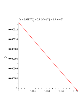
Figure 1: The graphical plot for radial pressure vs radius which has a definite cut-off at $4.17$ km

Let us now turn our attention to the physical analysis of the stellar model under consideration, i.e. whether it is a normal star or something else. To do so, primarily we try to figure out the radius of the stellar configuration. It is to note that in Eqs. (29), (34) and (39) the radius of the star $R$ has been mentioned under the boundary condition, $p_{r}(R)=0$, i.e. we get analytical results in the respective cases. So it seems that we can proceed on without further plot descriptions to get $p_{r}(R)=0$ for all dimensions. However, for $4D$ case it reveals that the radius of the star is very small with a numerical value of $4.17$ km (Fig. 1). This obviously then indicates that the star is nothing but a compact object (see Table 1 of all the Refs. Rahaman ; Kalam2012 ; Hossein2012 ; Kalam2013 for comparison with the radius of some of the real compact stars).

5 Matching conditions

Now, we match our interior solutions with the exterior vacuum solutions. The generalization of Schwarzschild solution, which as obtained by Tangherlini Tangherlini1963 reads as

$$ds^{2}=-\left(1-\frac{\mu_{n}}{r^{n-1}}\right)dt^{2}+\left(1-\frac{\mu_{n}}{r^{n-1}}\right)^{-1}dr^{2}+d\Omega_{n}^{2}.$$ (42)

Here,

$${\Omega}_{n}=\frac{2\pi^{\frac{n+1}{2}}}{\Gamma\left(\frac{n+1}{2}\right)},$$

the area of a unit $n$-sphere and

$$\mu_{n}=16\pi GM/nc^{2}{\Omega}_{n},$$

is the constant of integration with $M$, the mass of the black hole with $n=2,~{}3,~{}4,~{}9$.

5.1 Four dimensional spacetime ($n=2$)

For $4D$ case, our interior solution should match to the exterior Schwarzschild spacetime at the boundary $r=a_{4}$ given by

$$ds^{2}=-\left(1-\frac{\mu_{2}}{r}\right)dt^{2}+\left(1-\frac{\mu_{2}}{r}\right)^{-1}dr^{2}+r^{2}d\Omega_{2}.$$ (43)

Now using the matching conditions at the boundary $r=a_{4}$, we have

$$1-\frac{\mu_{2}}{a_{4}}=C_{2}^{2}a_{4}^{2},$$ (44)

and

$$1-\frac{\mu_{2}}{a_{4}}=1+\frac{A}{C_{3}^{2}a_{4}}-\frac{4M\sqrt{\phi}}{\pi a_{4}}\left[\frac{1}{\sqrt{\phi}}\arctan\left(\frac{a_{4}}{\sqrt{\phi}}\right)-\frac{a_{4}}{a_{4}^{2}+\phi}\right].$$ (45)

Solving the above two equations, we obtain

$$C_{2}^{2}=\frac{1}{a_{4}^{2}}\left(1-\frac{\mu_{2}}{a_{4}}\right),$$ (46)

$$\frac{A}{C_{3}^{2}}=\frac{4M\sqrt{\phi}}{\pi}\left[\frac{1}{\sqrt{\phi}}\arctan\left(\frac{a_{4}}{\sqrt{\phi}}\right)-\frac{a_{4}}{a_{4}^{2}+\phi}\right]-\mu_{2}.$$ (47)

5.2 Five dimensional spacetime ($n=3$)

For $5D$ case, our interior solution should match to the exterior $5D$ Schwarzschild spacetime at the boundary $r=a_{5}$, given by

$$ds^{2}=-\left(1-\frac{\mu_{3}}{r^{2}}\right)dt^{2}+\left(1-\frac{\mu_{3}}{r^{2}}\right)^{-1}dr^{2}+r^{2}d\Omega_{3}.$$ (48)

Now using the matching conditions at the boundary $r=a_{5}$, we have

$$1-\frac{\mu_{3}}{a_{5}^{2}}=C_{2}^{2}a_{5}^{2},$$ (49)

and

$$1-\frac{\mu_{3}}{a_{5}^{2}}=1+\frac{A}{C_{3}^{2}a_{5}^{2}}+\frac{16M\sqrt{\phi}}{9\pi a_{5}^{2}}\frac{3a_{5}^{2}+2\phi}{(a_{5}^{2}+\phi)^{\frac{3}{2}}}.$$ (50)

Solving the above two equations, we obtain

$$C_{3}^{2}=\frac{1}{a_{5}^{2}}\left(1-\frac{\mu_{3}}{a_{5}^{2}}\right),$$ (51)

and

$$\frac{A}{C_{3}^{2}}=-\mu_{3}-\frac{16M\sqrt{\phi}}{9\pi}\frac{3a_{5}^{2}+2\phi}{(a_{5}^{2}+\phi)^{\frac{3}{2}}}.$$ (52)

5.3 Six dimensional spacetime ($n=4$)

For $6D$ case, our interior solution should match to the exterior $6D$ Schwarzschild spacetime at the boundary $r=a_{6}$, given by

$$ds^{2}=-\left(1-\frac{\mu_{4}}{r^{3}}\right)dt^{2}+\left(1-\frac{\mu_{4}}{r^{3}}\right)^{-1}dr^{2}+r^{2}d\Omega_{4}.$$ (53)

Now using the matching conditions at the boundary $r=a_{6}$, we have

$$1-\frac{2\mu_{4}}{a_{6}^{3}}=C_{2}^{2}a_{6}^{2},$$ (54)

and

$$1-\frac{\mu_{4}}{a_{6}^{3}}=1-\frac{M\sqrt{\phi}}{2\pi a_{6}^{3}}\left[\frac{3}{\sqrt{\phi}}\tan^{-1}\left(\frac{a_{6}}{\sqrt{\phi}}\right)-\frac{5a_{6}^{3}+3a_{6}\phi}{(a_{6}^{2}+\phi)^{2}}\right]+\frac{A}{C_{3}^{2}a_{6}^{3}}.$$ (55)

Solving the above two equations, we obtain

$$C_{2}^{2}=\frac{1}{a_{6}^{2}}\left(1-\frac{\mu_{4}}{a_{6}^{3}}\right),$$ (56)

and

$$\frac{A}{C_{3}^{2}}=\frac{M\sqrt{\phi}}{2\pi}\left[\frac{3}{\sqrt{\phi}}\tan^{-1}\left(\frac{a_{6}}{\sqrt{\phi}}\right)-\frac{5a_{6}^{3}+3a_{6}\phi}{(a_{6}^{2}+\phi)^{2}}\right]-\mu_{4}.$$ (57)

5.4 Eleven dimensional spacetime ($n=9$)

For $11D$ case, our interior solution should match to the exterior 11D Schwarzschild spacetime at the boundary $r=a_{11}$, given by

$$ds^{2}=-\left(1-\frac{\mu_{9}}{r^{8}}\right)dt^{2}+\left(1-\frac{\mu_{9}}{r^{8}}\right)^{-1}dr^{2}+r^{2}d\Omega_{9}.$$ (58)

Now using the matching conditions at the boundary $r=a_{11}$, we have

$$1-\frac{\mu_{9}}{a_{11}^{8}}=C_{2}^{2}a_{11}^{2},$$ (59)

and

$$1-\frac{\mu_{9}}{a_{11}^{8}}=1+\frac{16M\sqrt{\phi}}{2835\pi a_{11}^{8}}\frac{315a_{11}^{8}+840a_{11}^{6}\phi+1008a_{11}^{4}\phi^{2}+576a_{11}^{2}\phi^{3}+128\phi^{4}}{(a_{11}^{2}+\phi)^{\frac{9}{2}}}+\frac{A}{C_{3}^{2}a_{11}^{8}}.$$ (60)

Solving the above two equations, we obtain

$$C_{2}^{2}=\frac{1}{a_{11}^{2}}\left(1-\frac{\mu_{9}}{a_{11}^{8}}\right),$$ (61)

and

$$\frac{A}{C_{3}^{2}}=\frac{M\sqrt{\phi}}{2\pi}\left[\frac{3}{\sqrt{\phi}}\tan^{-1}\left(\frac{a_{11}}{\sqrt{\phi}}\right)-\frac{5a_{11}^{3}+3a_{11}\phi}{(a_{11}^{2}+\phi)^{2}}\right]-\mu_{9},$$ (62)

where $a_{j}$ (j=4, 5, 6 and 11) are the radii of the fluid spheres in different dimensions.

6 A comparative study of the physical features of the model

Let us now carry out a comparative study of the physical features based on the solutions set obtained in the previous Section 4. This can be done in different ways. However, in the present investigation the best method we may adopt for comparative study, firstly, in connection to stability of the models for different dimensions which may be considered as most crucial one and secondly, for other physical parameters viz., density, pressure, pressure anisotropy, pressure gradient, conformal parameter and metric potential.

6.1 Stability of the stellar configuration

The Generalized Tolman-Oppenheimer-Volkoff (TOV) equation can be written in the form

$$-\frac{M_{G}(r)(\rho+p_{r})}{r^{2}}e^{\frac{\nu-\mu}{2}}-\frac{dp_{r}}{dr}+\frac{2}{r}(p_{t}-p_{r})=0,$$ (63)

where $M_{G}(r)$ is the gravitational mass within the sphere of radius $r$ and is given by

$$M_{G}(r)=\frac{1}{2}r\nu^{\prime}e^{\frac{\mu-\nu}{2}}.$$ (64)

Substituting (64) into (63), we obtain

$$-\frac{\nu^{\prime}}{2}(\rho+p_{r})-\frac{dp_{r}}{dr}+\frac{2}{r}(p_{t}-p_{r})=0.$$ (65)

The above TOV equation describe the equilibrium of the stellar configuration under gravitational force $F_{g}$, hydrostatic force $F_{h}$ and anisotropic stress $F_{a}$ so that we can write it in the following form:

$$F_{g}+F_{h}+F_{a}=0,$$ (66)

where

$$F_{g}=-\frac{\nu^{\prime}}{2}(\rho+p_{r}),$$

$$F_{h}=-\frac{dp_{r}}{dr},$$

$$F_{a}=\frac{2}{r}(p_{t}-p_{r}).$$

(67)

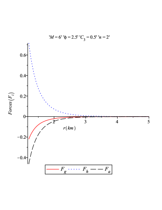
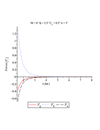
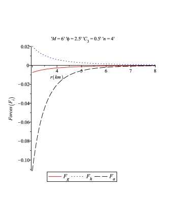
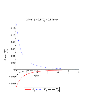
Figure 2: The three different forces namely gravitational forces $(F_{g})$, hydrostatic forces $(F_{h})$ and anisotropic forces $(F_{a})$ are plotted against $r$ (km) for $4D$ spacetime (top left), $5D$ spacetime (top right), $6D$ spacetime (bottom left) and $11D$ spacetime (bottom right). From the figure balancing status of the forces can be clearly observed for $4D$, $5D$, $6D$, $11D$ spacetimes

We have shown the plots of TOV equations for $4D$, $5D$, $6D$ and $11D$ spacetime in Fig. 2. From the plots it is overall clear that the system is in static equilibrium under three different forces, viz. gravitational, hydrostatic and anisotropic, for example, in the $4D$ case to attain equilibrium, the hydrostatic force is counter balanced jointly by gravitational and anisotropic forces. In $5D$ also the situation is exactly same, the only difference being in the radial distances. In $4D$ it is closer to 5 whereas in $5D$ it is closer to 8. This distance factor can also be observed in the higher dimensional spacetimes though the balancing features between the three forces are clearly different in the respective cases.

6.2 Energy conditions

Now we check whether all the energy conditions are satisfied or not. For this purpose, we shall consider the following inequalities:

$$(i)~{}NEC:\rho+p_{r}\geq 0,~{}\rho+p_{t}\geq 0,$$

$$(ii)~{}WEC:\rho+p_{r}\geq 0,~{}\rho\geq 0,~{}\rho+p_{t}\geq 0,$$

$$(iii)~{}SEC:\rho+p_{r}\geq 0,~{}\rho+p_{r}+2p_{t}\geq 0.$$

Fig. 3 indicates that in our model all the energy conditions are satisfied through out the interior region.

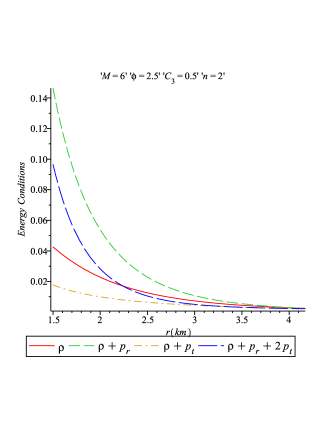
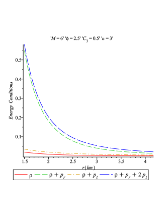
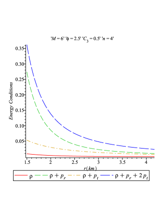
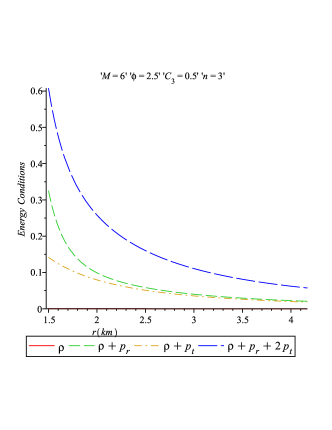
Figure 3: The energy conditions in the interior have been plotted against $r$ for $4D$ spacetime (top left), $5D$ spacetime (top right), $6D$ spacetime (bottom left) and $11D$ spacetime (bottom right)

6.3 Anisotropy of the models

We have shown the possible variation of radial and transverse pressures in Fig. 4 (top left and right of the panel respectively). Hence the measure of anisotropy $\Delta=(p_{t}-p_{r})$ in $4$, $5$, $6$ and $11$ dimensional cases are respectively given as

$$\Delta_{4}=\frac{1}{8\pi}\left[\frac{12M\sqrt{\phi}}{\pi r^{3}}\left\{\frac{1}{\sqrt{\phi}}\arctan\left(\frac{r}{\sqrt{\phi}}\right)-\frac{r}{r^{2}+\phi}\right\}-\frac{1}{r^{2}}-\frac{8M\sqrt{\phi}}{\pi(r^{2}+\phi)^{2}}-\frac{3A}{C_{3}^{2}r^{3}}\right],$$ (68)

$$\Delta_{5}=\frac{1}{8\pi}\left[\frac{32M\sqrt{\phi}}{3\pi r^{4}}\left\{\frac{3r^{2}+2\phi}{(r^{2}+\phi)^{\frac{3}{2}}}\right\}-\frac{1}{r^{2}}-\frac{8M\sqrt{\phi}}{\pi(r^{2}+\phi)^{\frac{5}{2}}}+\frac{6A}{C_{3}^{2}r^{4}}\right],$$ (69)

$$\Delta_{6}=\frac{1}{8\pi}\left[\frac{5M\sqrt{\phi}}{\pi r^{5}}\left\{\frac{3}{\sqrt{\phi}}\tan^{-1}\left(\frac{r}{\sqrt{\phi}}\right)-\frac{5r^{3}+3r\phi}{(r^{2}+\phi)^{2}}\right\}-\frac{1}{r^{2}}-\frac{8M\sqrt{\phi}}{\pi(r^{2}+\phi)^{3}}-\frac{10A}{r^{5}C_{3}^{2}}\right],$$ (70)

$$\Delta_{11}=\frac{1}{8\pi}\left[\frac{M\sqrt{\phi}}{4\pi r^{10}}\left\{\frac{315r^{8}+840r^{6}\phi+1008r^{4}\phi^{2}+576r^{2}\phi^{3}+128\phi^{4}}{(r^{2}+\phi)^{\frac{9}{2}}}\right\}\right.$$

$$-\left.\frac{1}{r^{2}}-\frac{8M\sqrt{\phi}}{\pi(r^{2}+\phi)^{\frac{11}{2}}}+\frac{45A}{C_{3}^{2}r^{10}}\right],$$ (71)

All these are plotted in Fig. 4 (bottom left of the panel). From all the plots we see that $\Delta<0$  i.e., $p_{t}~{}<p_{r}$ and hence the anisotropic force is attractive in nature. A detailed study shows that firstly, in every case of different dimensions the measure of anisotropy is a decreasing function of $r$. Secondly, from $4D$ onward measure of anisotropy is increasing gradually and is attaining maximum at $5D$. Surprisingly, it is very high compared to $4D$ and $11D$ spacetimes. This observation therefore dictates that $4D$ configuration represents almost a spherical object as departure from isotropy is very less than the higher dimensional spacetimes.

Moreover, in all the above cases of different dimension one can note that the pressure gradient $\frac{dp_{r}}{dr}$ is a decreasing function of $r$ (bottom right panel of Fig. 4).

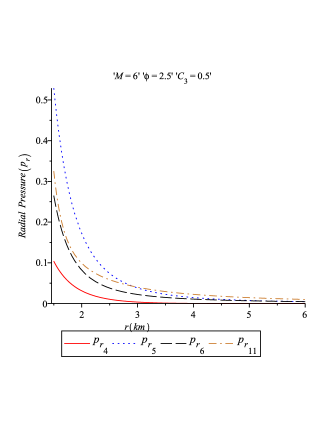
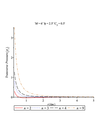
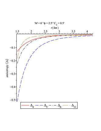
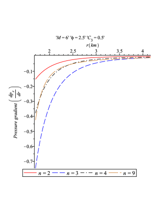
Figure 4: Variation of the radial pressure $p_{r}$ in the interior of the compact star in $4D$, $5D$, $6D$, $11D$ have been plotted against $r$ (Left). The figures show that profiles of $p_{r}$ are monotonic decreasing function of $r$. The anisotropic factor $\Delta$ for $4D$, $5D$, $6D$, $11D$ cases are shown against $r$ (right). In both the cases the suffixes in the legends indicate the dimension of the spacetime

6.4 Compactness and redshift of the star

At the end of previous Section we did a primary test to get a preliminary idea about the structure of the star under consideration and we have seen that the star actually represents a compact object with a radius $4.17$ km. However, for further test of confirmation one can perform some specific calculations for ‘compactness factor’ Rahaman ; Kalam2012 ; Hossein2012 ; Kalam2013 .

To do so we first define gravitational mass of the system of matter distribution as follows:

$$m(r)=\int_{0}^{r}~{}\left[\frac{2\pi^{\frac{n+1}{2}}}{\Gamma\left(\frac{n+1}{2}\right)}\right]r^{n}\rho dr.$$ (72)

Therefore, the compactness factor and surface redshift of the star can be respectively given by

$$u(r)=\frac{m(r)}{r},$$ (73)

$$z_{s}=[1-2u]^{-1/2}-1.$$ (74)

Hence for different dimensions we can calculate the expressions for the above parameters as follows:

For n=2:

$$m(r)=\frac{2M}{\pi}\left[tan^{-1}\left(\frac{r}{\sqrt{\phi}}\right)-\frac{r\sqrt{\phi}}{r^{2}+\phi}\right],$$ (75)

$$u(r)=\frac{2M}{\pi r}\left[tan^{-1}\left(\frac{r}{\sqrt{\phi}}\right)-\frac{r\sqrt{\phi}}{r^{2}+\phi}\right],$$ (76)

$$z_{s}=\left[1-\frac{4M}{\pi r}\left\{tan^{-1}\left(\frac{r}{\sqrt{\phi}}\right)-\frac{r\sqrt{\phi}}{r^{2}+\phi}\right\}\right]^{-\frac{1}{2}}-1.$$ (77)

For n=3:

$$m(r)=\frac{2M}{3}\left[2-\frac{(3r^{2}+2\phi)\sqrt{\phi}}{(r^{2}+\phi)^{\frac{3}{2}}}\right],$$ (78)

$$u(r)=\frac{2M}{3r}\left[2-\frac{(3r^{2}+2\phi)\sqrt{\phi}}{(r^{2}+\phi)^{\frac{3}{2}}}\right],$$ (79)

$$z_{s}=\left[1-\frac{4M}{3r}\left\{2-\frac{(3r^{2}+2\phi)\sqrt{\phi}}{(r^{2}+\phi)^{\frac{3}{2}}}\right\}\right]^{-\frac{1}{2}}-1.$$ (80)

For n=4:

$$m(r)=M\left[tan^{-1}\left(\frac{r}{\sqrt{\phi}}\right)-\frac{r\sqrt{\phi}(5r^{2}+3\phi)}{3(r^{2}+\phi)^{2}}\right],$$ (81)

$$u(r)=M\left[\frac{1}{r}tan^{-1}\left(\frac{r}{\sqrt{\phi}}\right)-\frac{\sqrt{\phi}(5r^{2}+3\phi)}{3(r^{2}+\phi)^{2}}\right],$$ (82)

$$z_{s}=\left[1-2M\left\{\frac{1}{r}tan^{-1}\left(\frac{r}{\sqrt{\phi}}\right)-\frac{\sqrt{\phi}(5r^{2}+3\phi)}{3(r^{2}+\phi)^{2}}\right\}\right]^{-\frac{1}{2}}-1.$$ (83)

For n=9:

$$m(r)=\frac{M\pi^{3}}{3780}\left[128-\frac{128\phi^{4}+576\phi^{3}r^{2}+1008\phi^{2}r^{4}+840\phi r^{6}+315r^{8}}{(r^{2}+\phi)^{\frac{9}{2}}}\sqrt{\phi}\right],$$ (84)

$$u(r)=\frac{M\pi^{3}}{3780r}\left[128-\frac{128\phi^{4}+576\phi^{3}r^{2}+1008\phi^{2}r^{4}+840\phi r^{6}+315r^{8}}{(r^{2}+\phi)^{\frac{9}{2}}}\sqrt{\phi}\right],$$ (85)

$$z_{s}=\left[1-\frac{M\pi^{3}}{1890r}\left\{128-\frac{128\phi^{4}+576\phi^{3}r^{2}+1008\phi^{2}r^{4}+840\phi r^{6}+315r^{8}}{(r^{2}+\phi)^{\frac{9}{2}}}\sqrt{\phi}\right\}\right]^{-\frac{1}{2}}-1.$$ (86)

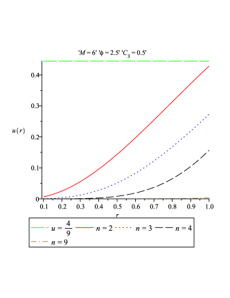
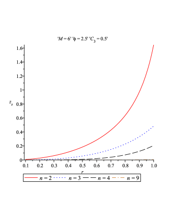
Figure 5: The compactness factor (left) and surface redshift (right) of compact star in $4D$, $5D$, $6D$, $11D$ dimensions are plotted against $r$ (km) for the specified range

The nature of variation of the above expressions for compactness factor and surface redshift of the star can be seen in the Fig. 5 in the left and right panel respectively for all the values of $n$. It is observed from Fig. 5 (left panel) that compactness factors for different dimensions are gradually increasing with decreasing $n$ and maximum for $4D$ spacetime. Thus, very interestingly, at the center the star is most dense for $4$-dimension with a very small yet definite core whereas in the $11D$ case here seem to be no core.

We note that in connection with the isotropic case and in the absence of the cosmological constant it has been shown for the surface redshift analysis that $z_{s}\leq 2$ Buchdahl1959 ; Straumann1984 ; Boehmer2006 . On the other hand, Böhmer and Harko Boehmer2006 argued that for an anisotropic star in the presence of a cosmological constant the surface redshift must obey the general restriction $z_{s}\leq 5$, which is consistent with the bound $z_{s}\leq 5.211$ as obtained by Ivanov Ivanov2002 . Therefore, for an anisotropic star without cosmological constant the above value $z_{s}\leq 1$ is quite reasonable as can be seen in the $4D$ case (Fig. 5, right panel) Rahaman . In the other cases of higher dimension the surface redshift values are increasing and seem to be within the upper bound Ivanov2002 .

We note that integration of $m(r)$ from $0$ to $R$, where $R$ is the radius of the fluid distribution, gives $M$ (total mass of the source) i.e.

$$M=\int_{0}^{R}~{}\left[\frac{2\pi^{\frac{n+1}{2}}}{\Gamma\left(\frac{n+1}{2}\right)}\right]r^{n}\rho dr.$$

This equation gives the radius $R$ of the fluid distribution. Thus solutions of the following equations provide the corresponding radius of different dimensional situations.

For $n=2$:

$$M=\frac{2M}{\pi}\left[tan^{-1}\left(\frac{R}{\sqrt{\phi}}\right)-\frac{R\sqrt{\phi}}{R^{2}+\phi}\right],$$ (87)

For $n=3$:

$$M=\frac{2M}{3}\left[2-\frac{(3R^{2}+2\phi)\sqrt{\phi}}{(R^{2}+\phi)^{\frac{3}{2}}}\right],$$ (88)

For $n=4$:

$$M=M\left[tan^{-1}\left(\frac{R}{\sqrt{\phi}}\right)-\frac{R\sqrt{\phi}(5R^{2}+3\phi)}{3(R^{2}+\phi)^{2}}\right],$$ (89)

For $n=9$:

$$M=\frac{M\pi^{3}}{3780}\left[128-\frac{128\phi^{4}+576\phi^{3}R^{2}+1008\phi^{2}R^{4}+840\phi R^{6}+315R^{8}}{(R^{2}+\phi)^{\frac{9}{2}}}\sqrt{\phi}\right],$$ (90)

6.5 Some other physical parameters

In this subsection we have shown the panel of the plots for the conformal parameter $\psi(r)$ (top left), the metric potential $e^{\lambda}$ (top right) and the density $\rho$ (bottom) for $4$ and extra dimensional spacetimes (Fig. 6). It is observed that for all the physical parameters the features are as usual for $4D$, however for extra dimension they take different shapes. A special mention can be done for density where central densities are abruptly decreasing as one goes to higher dimensions. Thus, from the plot it reveals that the central density is maximum for $4D$ whereas it is minimum for $11D$ spacetime showing most compactness of the star for standard $4$-dimension. Note that this same result was observed in Fig 5 (left panel).

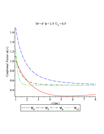
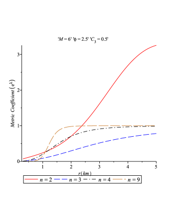
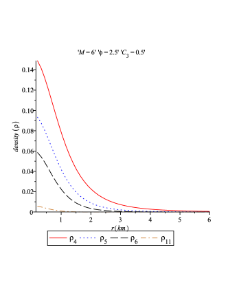
Figure 6: The conformal factor $\psi(r)$ (top left), the metric potential $e^{\lambda}$ (top right) and matter density (bottom) are plotted against $r$ (km) for $4D$, $5D$, $6D$, $11D$ dimensional spacetimes. The suffixes in the left panel indicates the dimension of the spacetime and for right panel $D=n+2$ stands for the dimension of the spacetime

7 Conclusion

In the present paper we have studied thoroughly a set of new interior solutions for anisotropic stars admitting conformal motion in higher dimensional noncommutative spacetime. Under this spacetime geometry the Einstein field equations are solved by choosing a particular Lorentzian type density distribution function as proposed by Nozari and Mehdipour Nozari2009 . The studies are conducted not only with standard $4D$ dimensional spacetime but also for three special cases with higher dimension, such as $5D$, $6D$ and $11D$. In general it is noted that the model parameters e.g. matter-energy density, radial as well as transverse pressures, anisotropy and others show physical behaviours which are mostly regular throughout the stellar configuration.

Also it is specially observed that the solutions represent a star with mass $2.27$ $M_{\odot}$ and radius $4.17$ km which falls within the range ($0<z_{s}\leq 1$) of a compact star Rahaman ; Kalam2012 ; Hossein2012 ; Kalam2013 . However, it has been shown that for a strange star of radius $6.88$ km surface redshift turns out to be $z_{s}=0.5303334$ Rahaman whereas the maximum surface redshift for a strange star $HerX-1$ of radius $7.7$ km is $0.022$ Kalam2012 and that for a compact star $4U~{}1820-30$ of radius $10$ km turns out to be again $0.022$ Hossein2012 . Therefore it seems that our compact star may be a strange quark star (see Table 1).

Table 1: Values of the model parameter $z_{s}$ for different Strange Stars

Strange Star candidates	$M$($M_{\odot}$)	$R$(km)	$M/R$	$z_{s}$
Her X-1	0.88	7.7	0.168	0.0220 [Ref. 13]
				0.2285 [Ref. 15]
4U 1820-30	2.25	10.0	0.332	0.0220 [Ref. 14]
				0.7246 [Ref. 15]
SAX J 1808.4-3658(SS1)	1.435	7.07	0.299	0.5787 [Ref. 15]
SAX J 1808.4-3658(SS2)	1.323	6.35	0.308	0.6108 [Ref. 15]
Rahaman model [Ref. 11]	1.46	6.88	0.313	0.5303334
Our proposed model	2.27	4.17	0.804	$0<z_{s}\leq 1$

However, through several mathematical case studies we have given emphasis on the acceptability of the model from physical point of view for various structural aspects. As a consequence it is observed that for higher dimensions, i.e. beyond $4D$ spacetime, the solutions exhibit several interesting yet bizarre features. These features seem physically not very unrealistic.

Thus, as a primary stage, the investigation indicates that compact stars may exist even in higher dimensions. But before placing a demand in favour of this highly intrigued issue of compact stars with extra dimensions we need to perform more specific studies and to look at the diversified technical aspects related to higher dimensional spacetimes of a compact star. Basically our approach, dependent on a particular energy density distribution of Lorenztian type, which gives higher dimensional existence of compact stars may not be only the way to have sufficient evidence in favour of it. We further need to employ other type of density distributions as well. Moreover, one may also think for other than higher dimensional embedding of GTR and thus opt for alternative theories of gravity to find conclusive proof for higher dimensional compact stars.

However, in the literature there are some evidences available in favour of ‘Extra Dimensions in Compact Stars’ Liddle1990 ; BLL2003 ; Paul2004 ; BLL2006 ; BLL2010 ; CP2010 .

References

• (1) K. Nozari, S.H. Mehdipour, JHEP 0903, 061 (2009)
• (2) S.H. Mehdipour, Eur. Phys. J. Plus 127, 80 (2012)
• (3) R. Ruderman, Rev. Astr. Astrophys. 10, 427 (1972)
• (4) M.K. Gokhroo, A.L. Mehra, Gen. Relativ. Grav. 26, 75 (1994)
• (5) R. Kippenhahn, A. Weigert, Steller Structure and Evolution, Springer-Verlag (1990)
• (6) A.I. Sokolov, JETP 79, 1137 (1980)
• (7) R.F. Sawyer, Phys. Rev. Lett. 29, 382 (1972); Erratum Phys. Rev. Lett. 29, 823 (1972)
• (8) R.L. Bowers, E.P.T. Liang, Astrophys. J. 188, 657 (1917)
• (9) V. Varela, F. Rahaman, S. Ray, K. Chakraborty, M. Kalam, Phys. Rev. D 82, 044052 (2010)
• (10) F. Rahaman, S. Ray, A.K. Jafry, K. Chakraborty, Phys. Rev. D 82, 104055 (2010)
• (11) F. Rahaman, R. Sharma, S. Ray, R. Maulick, I. Karar, Eur. Phys. J. C 72, 2071 (2012)
• (12) F. Rahaman, R. Maulick, A.K. Yadav, S. Ray, R. Sharma, Gen. Rel. Grav. 44, 107 (2012)
• (13) M. Kalam, F. Rahaman, S. Ray, M. Hossein, I. Karar, J. Naskar, Euro. Phys. J. C 72, 2248 (2012)
• (14) Sk. M. Hossein, F. Rahaman, J. Naskar, M. Kalam, S. Ray, Int. J. Mod. Phys. D 21, 1250088 (2012)
• (15) M. Kalam, A.A. Usmani, F. Rahaman, S.M. Hossein, I. Karar, R. Sharma, Int. J. Theor. Phys. 52, 3319 (2013)
• (16) F. Rahaman, S. Ray, M. Kalam, M. Sarker, Int. J. Theor. Phys. 48, 3124 (2009)
• (17) H. Liu, J.M. Overduin, Astrophys. J. 538, 386 (2000)
• (18) F. Rahaman, S. Chakraborty, S. Ray, A.A. Usmani, S. Islam, Int. J. Theor. Phys. 54 , 50 (2015)
• (19) E. Witten, Nucl. Phys. B 460, 335 (1996)
• (20) N. Seiberg, E. Witten, JHEP 032, 9909 (1999)
• (21) A. Smailagic, E. Spallucci, J. Phys A 36, L467 (2003)
• (22) F. Rahaman, P.K.F Kuhfittig, K. Chakraborty, A.A. Usmani, S. Ray, Gen. Relativ. Gravit. 44, 905 (2012)
• (23) P.K.F Kuhfittig, Adv. High Energy Phys. 2012, 462493 (2012)
• (24) F. Rahaman, S. Islam, P.K.F Kuhfittig, S. Ray, Phys. Rev. D 86, 106010 (2012)
• (25) F. Rahaman, P.K.F. Kuhfittig, B.C. Bhui, M. Rahaman, S. Ray, U.F. Mondal, Phys. Rev. D 87, 084014 (2013)
• (26) F. Rahaman, S. Ray, G.S. Khadekar, P.K.F. Kuhfittig, I. Karar, Int. J. Theor. Phys. (in press), DOI 10.1007/s10773-014-2262-y (2014)
• (27) F. Rahaman, A. Banerjee, M. Jamil, A.K. Yadav, H. Idris, Int. J. Theor. Phys. 53, 1910 (2014)
• (28) C.G. Böhmer, T. Harko, F.S.N. Lobo, Phys. Rev. D 76, 084014 (2007)
• (29) C.G. Böhmer, T. Harko, F.S.N. Lobo, Class. Quantum Gravit. 25, 075016 (2008)
• (30) F. Rahaman, M. Jamil, R. Sharma, K. Chakraborty, Astrophys. Space Sci. 330, 249 (2010)
• (31) F. Rahaman, A. Pradhan, N. Ahmed, S. Ray, B. Saha, M. Rahaman, arXiv: gr-qc 1401.1402.
• (32) A.A. Usmani, F. Rahaman, S. Ray, K.K. Nandi, P.K.F. Kuhfittig, Sk.A. Rakib, Z. Hasan, Phys. Lett. B 701, 388 (2011)
• (33) P. Bhar, Astrophys. Space Sci. 354, 457 (2014)
• (34) F. Rahaman, M. Jamil, M. Kalam, K. Chakraborty, A. Ghosh, Astrophys. Space Sci. 137, 325 (2010)
• (35) E. Spallucci, A. Smailagic, P. Nicolini, Phys. Rev. D 73, 084004 (2006)
• (36) R. Banerjee, B. Chakraborty, S. Ghosh, P. Mukherjee, S. Samanta, Found. Phys. 39, 1297 (2009)
• (37) L. Modesto, P. Nicolini, Phys. Rev. D 81, 104040 (2010)
• (38) P. Nicolini, M. Rinaldi, Phys. Lett. B 695, 303 (2011)
• (39) F.S.N. Lobo, Classical and Quantum Gravity Research Progress, pp. 1-78, Nova Sci. Pub. (2008)
• (40) F. R. Tangherlini, Nuo. Cim. 27 (1963) 636.
• (41) H.A. Buchdahl, Phys. Rev. 116, 1027 (1959)
• (42) N. Straumann, General Relativity and Relativistic Astrophysics, Springer-Verlag, Berlin (1984)
• (43) C.G. Böhmer and T. Harko, Class. Quantum Gravit. 23, 6479 (2006)
• (44) B.V. Ivanov, Phys. Rev. D 65, 104011 (2002)
• (45) A.R. Liddle, R.G. Moorhouse, A.B. Henriques, Class. Quantum Grav. 7, 1009 (1990)
• (46) G.G. Barnaföldi, P. Lévai, B. Lukács, arXiv: astro-ph/0312330 (2003)
• (47) B.C. Paul, Int. J. Mod. Phys. D 13, 229 (2004)
• (48) G.G. Barnaföldi, P. Lévai, B. Lukács, Astron. Nachr. 999, 789 (2006)
• (49) G.G. Barnaföldi, P. Lévai, B. Lukács, J. Phys.: Conf. Series 218, 012010 (2010)
• (50) P.K. Chattopadhyay, B.C. Paul, Pramana: J. Phys. 74, 513 (2010)