The transmission coefficient distribution of highly scattering sparse random media
Curtis Jin, Raj Rao Nadakuditi, Eric Michielssen
(jsirius@umich.edu, rajnrao@umich.edu, emichiel@umich.edu
Abstract
We consider the distribution of the transmission coefficients, i.e. the singular values of the modal transmission matrix, for 2D random media with periodic boundary conditions composed of a large number of point-like nonabsorbing scatterers. The scatterers are placed at random locations in the medium and have random refractive indices that are drawn from an arbitrary, known distribution. We construct a randomized model for the scattering matrix that retains scatterer dependent properties essential to reproduce the transmission coefficient distribution and analytically characterize the distribution of this matrix as a function of the refractive index distribution, the number of modes, and the number of scatterers. We show that the derived distribution agrees remarkably well with results obtained using a numerically rigorous spectrally accurate simulation. Analysis of the derived distribution provides the strongest principled justification yet of why we should expect perfect transmission in such random media regardless of the refractive index distribution of the constituent scatterers. The analysis suggests a sparsity condition under which random media will exhibit a perfect transmission-supporting universal transmission coefficient distribution in the deep medium limit.
OCIS codes: 030.6600
1 Introduction
Materials such as turbid water, white paint, and egg shells are considered opaque because multiple scattering by the randomly placed constituent scatterers in the medium frustrates the passage of light [11]. The seminal papers by Dorokhov [8], Barnes and Pendry et al. [18, 3], and others [17, 4] postulate that even if a normally incident wavefront barely propagates through a thick slab of such media, there will generically exist a few highly-transmitting wavefronts that will propagate through the slab with a transmission coefficient close to , i.e, they will be nearly perfectly-transmitting. These perfectly transmitting eigen-wavefronts are the right singular vectors of the modal transmission matrix and are optimized to the specific random medium.
These seminal papers inspired the breakthrough experiments by Vellekoop and Mosk [26, 27], and others [19, 15, 21, 14, 25, 2, 6, 7, 24] provide credence to the hypothesis that there generally exist (nearly) perfectly transmitting eigen-wavefronts in highly scattering random media composed of a larger number of non-absorbing scatterers. Recently, we verified this hypothesis [12, 13] for 2-D systems with periodic boundary conditions composed of hundreds of thousands of non-absorbing scattering using numerically rigorous simulations.
The perfect-transmission supporting universal transmission coefficient distribution postulated by Dorokhov, Mello, Pereyra, Kumar, Pendry, and Barnes [8, 18, 3, 17], was derived assuming that the medium was deep enough so that the scattering matrix obeyed a physically consistent (i.e. obeying reciprocity and time-reversal conditions) maximum-entropy law. Their analysis does not provide a principled and mathematically grounded framework for reasoning about whether, when or the sense in which a deep medium composed of a large number of randomly placed point-like scatterers with an arbitrary distribution of refractive indices can be expected to have a perfect transmission-supporting transmission coefficient distribution.
In this paper, we use modern random matrix theory to revisit the problem of predicting the transmission coefficient distribution of 2-D random media with periodic boundary conditions composed of a larger number of randomly placed point-like scatterers with an arbitrary refractive index distribution. We provide a characterization of the transmission coefficient distribution that explicitly depends on the refractive index distribution, the number of propagating modes and the depth of the medium for layered random media (in a sense we will make precise) composed of a large number of point-like scatterers.
The critical part of our derivation relies on the development of an isotropic random matrix model for the modal transfer matrix of a single randomly placed point-like scatterer. The random transfer matrix has singular value distribution that matches the singular values of the physical transfer matrix of a randomly-placed point-like scatterer. However, the left and right singular vectors of our random transfer matrix construction are modeled as independent and isotropically random. This allows us to use tools from free probability theory to approximate the transmission coefficient distribution of a layered random media composed of layers containing point-like scatterers.
We show that the derived distribution agrees remarkably well with results obtained using a numerically rigorous spectrally convergent simulation that utilizes spectrally accurate methodologies. This justifies the use of our isotropic model for reasoning about the properties of the derived distribution. Analysis of the resulting distribution brings into sharp focus the universal, i.e., scatterer-property independent, aspects of the distribution and provides the strongest principled justification yet of why we should expect perfect transmission in such deep random media regardless of the refractive index distribution of the constituent scatterers. The analysis brings into focus a sparsity condition under which random media can be expected to exhibit a perfect transmission-supporting universal transmission coefficient distribution in the deep medium limit.
We describe the setup and define the transmission coefficient distribution in Section 2 . We highlight some pertinent properties of the system modal transfer matrix in Section 3, and employ them in Section 4 to formulate a isotropically random model for the transfer matrix of a single point-like scatterer. In Section 5, we describe the pertinent free probabilistic tools from random matrix theory that allow us to analytically characterize the limiting transmission coefficient distribution of a medium composed of many scatterers from the eigen-distribution of the isotropic transfer matrix of a single point-like scatterer. We analyze the properties of the limiting transmission coefficient distribution thus obtained in Section 6, and bring into sharp focus its universal, i.e., scatterer property independent, aspects. We validate our theoretical predictions using numerically rigorous simulations in Section 7. Details of some computations have been relegated to the Appendix.
2 Setup
We study scattering from a two-dimensional (2D) random slab of thickness and periodicity ; the slab’s unit cell occupies the space and (Fig. 1). The slab contains infinite and -invariant circular cylinders of radius that are placed randomly within the cell, as described shortly. The cylinders are assumed to be dielectric with refractive index ; care is taken to ensure the cylinders do not overlap. The radius of the cylinders is chosen to be much smaller than the wavelength so they, in effect, act like point scatterers.
For , the and position of the center of the -th cylinder are , respectively where and s are i.i.d, random variables with uniform distribution on and , respectively. Here is depth of each “layer”; is chosen to be larger than . Each cylinder’s refractive index is drawn independently from the same distribution of refractive indices .
Fields are polarized: electric fields in the and halfspaces are denoted . The field amplitude can be decomposed in terms of and propagating waves as , where
| (1) |
In the above expression, , , , , is the wavelength, and is a power-normalizing coefficient; a time dependence is assumed and suppressed. We assume , i.e. we only model propagating waves and denote . The modal coefficients , ; are related by the scattering matrix
| (2) |
where . In what follows, we assume that the slab is only excited from the halfspace; hence, . For a given incident field amplitude , we define the transmission coefficient as
| (3) |
We denote the transmission coefficient of a normally incident wavefront by ; here T denotes transposition.
2.A The transmission coefficient distribution
The problem of designing an incident wavefront that maximizes the transmitted power can be stated as
| (4) |
where represents an incident power constraint.
Let denote the singular value decomposition (SVD) of ; is the singular value associated with the left and right singular vectors and , respectively. By convention, the singular values are arranged so that and H denotes complex conjugate transpose. Then via a well-known result for the variational characterization of the largest right singular vector [10, Theorem 7.3.10] we have that
| (5) |
When the optimal wavefront is excited, the transmitted power is . When the wavefront associated with the -th right singular vector is transmitted, the transmitted power is , which we refer to as the transmission coefficient of the -th eigen-wavefront of . We are interested in the limiting transmission coefficient distribution whose p.d.f. is defined as
| (6) |
where we assume that as . The Dorokhov-Mello-Pereyra-Kumar (henceforth, DMPK) distribution [8, 17] has density given by
| (7) |
where is the mean-free path in the medium. The DMPK distribution is posited [8, 18, 3, 17, 4] to be the universal limiting distribution for systems comprised of many scatterers in the limit where .
Assuming a scattering regime where the DMPK distribution holds, Eq. (7) predicts the existence of highly-transmitting eigen-wavefronts that achieve (nearly) perfect transmission. Since the DMPK distribution was derived under a maximum-entropy type assumption (which we shall revisit shortly), the material properties of the scatterers, such as the distribution of refractive indices, do not explicitly appear in the expression in Eq. (7) for its p.d.f. but instead are encoded implicitly via the parameter. Our objective is to theoretically predict in Eq. (6) and explicitly characterize its dependence on the refractive index distribution , , and , assuming we are in a regime where each scatterer is small enough so that it effectively acts as an isotropic point scatterer. Our mathematically-derived framework permits reasoning about the conditions under which we might expect a universal limiting distribution and the existence of the (nearly) perfectly transmitting eigen-wavefronts.
3 Background: the transfer matrix and its pertinent properties
The scattering matrix in Eq. (2) describes the relationship between the modal coefficients of incoming and outgoing waves. Rearranging the terms in Eq. (2) relates the modal coefficients in and halfspace via the transfer matrix
| (8) |
where we have assumed that the matrix is invertible. Rewriting the transfer matrix as
| (9) |
allows us to easily verify that . In the lossless setting when , and is invertible, it is shown in Appendix A that the eigenvalues of denoted by are
| (10) |
Note that so that the eigenvalues of come in reciprocal pairs. From Eq. (10), we have that
so that
| (11) |
Substituting in Eq. (11) yields
Equivalently, since , we have
| (12) |
and we have obtained a direct relationship between the eigenvalues of and the transmission coefficients. Let denote the limiting eigenvalue distribution of the transfer matrix defined as
| (13) |
Then, a direct consequence of Eq. (12) is that once we know , a simple change of variables yields the transmission coefficient distribution as
| (14) |
Since the eigenvalues of come in reciprocal pairs, for uniquely determines for . Thus we can rewrite Eq. (14) as
| (15) |
where denotes the indicator function on the set . From Eq. (11), we have that
so that rearranging terms on the right hand side of Eq. (15), yields
| (16) |
We note that Eq. (16) is an exact relationship between the eigenvalue distribution of the transfer matrix and the transmission coefficient distribution. Comparing Eqs. (16) and (7) reveals the important insight that the DMPK distribution arises under the assumption that in the limit of deep random media, , or equivalently, that is a log-uniform distribution. This is the maximum-entropy assumption that yields the DMPK distribution for deep random media. Our goal is to analytically characterize and hence , via Eq. (16) as a function of , and the refractive index distribution of the scatterers for the setup in Fig. 1.
4 An isotropically random model for the transfer matrix of a single point-like scatterer
Let denote the transfer matrix of a layer containing a single scatterer (Fig. 1) and let , , , and denote its scattering matrix and subblocks thereof, respectively. When the scatterers are point-like and is large, then and are well approximated by a rank one matrix whose largest singular value we will refer to as the scattering strength. This is obviously true for , and remains remarkably accurate for smaller as well. Since is unitary for lossless media, we have that . Hence, the matrix must have an SVD of the form
where and are the left and right singular vectors of , which encode the physics of the scattering system. Consequently, by Eq. (3), the transmission coefficients of are approximately
From Eq. (10), we can conclude that the eigenvalues of will equal one. The remaining two eigenvalues will and where
| (17) |
This implies that the transfer matrix will have an SVD of the form
| (18) |
where and are the left and right singular vectors of , which again encode the physics of the scattering systems. The refractive index distribution induces a distribution on which we assume to known and obtained either a via a change of variables as
| (19) |
under a point scatterer assumption for the large , , and regime, or using computational electromagnetic techniques.
The transfer matrix of the entire system in Fig. 1 is obtained from those of the layers as
| (20) |
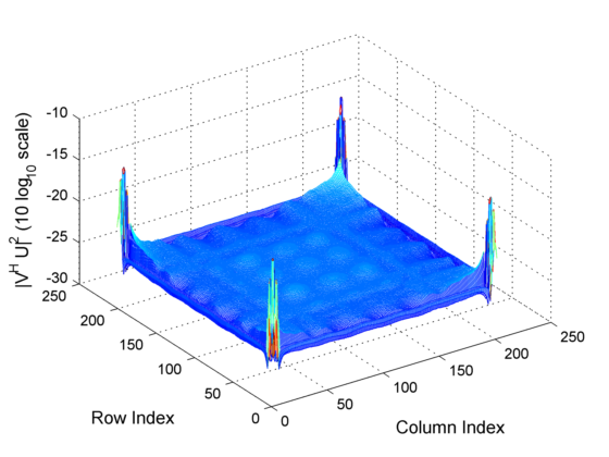
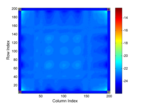
Each of the transfer matrices are independent and identically distributed. Fig. 2 plots the expected values of the squared magnitude of the (bistochastic) correlation matrix formed by the inner product of the right singular vectors of a transfer matrix associated with a single randomly placed scatterer and the left singular vectors of an independent transfer matrix associated with another randomly placed scatter, averaged over independent realizations. If the singular vectors were independent and isotropically random (or Haar distributed) then we would get an empirically averaged matrix with all of its entries close to . From Fig. 2, we can conclude that the singular vectors of two independent transfer matrices are not isotropically random with respect to each other. However, most of the entries of the correlation matrix have entries ‘close’ to .
Very recently, Anderson and Farrell [1] rigorously showed that the product of independent (Hermitian) random matrices with independent eigenvectors having a correlation matrix whose entries have squared magnitude entries exactly equal to will have the same limiting distribution as the product of independent random matrices with the same eigenvalue distribution but isotropically random eigenvectors. Here too, we have a situation where we are interested in analyzing the singular value distribution of products of random matrices with independent singular vectors. However, the correlation matrix of the singular vectors has entries whose squared magnitude is not exactly , as would be the case if the left and right singular vectors were isotropically random, but instead close to . This leads to our conjecture that the singular value distribution of the matrix in Eq. (20) can be ‘well approximated by’ the singular value distribution of independent random matrices with the same per-matrix singular value distribution but isotropically random left and right singular vectors.
Motivated by this conjecture, we now consider an isotropic random matrix model for the transfer matrices whose singular values are specified by Eq. (18) but whose left and right singular vectors are independent and isotropically random. We then use tools from free probability theory to analytically characterize the transmission coefficient distribution that arises due to this isotropic model for the transfer matrix of a point-like scatterer. Numerically rigorous physical simulations in Section 7 will validate our conjecture. A mathematically rigorous treatment of this conjecture, including a quantification of the approximation error, remains an open problem.
5 Analytically characterizing the transmission coefficient distribution
We now discuss some preliminaries required to compute the transmission coefficient distribution under the isotropic transfer matrix assumption. Let be an symmetric (or Hermitian) random matrix whose ordered eigenvalues are denoted by . Let be the empirical eigenvalue distribution, i.e. , the probability distribution with density
Now suppose that and are two independent matrices whose empirical eigenvalue distributions converge as to non-random distributions having densities and , respectively. A natural question then is: how is the limiting eigenvalue distribution of the matrix related to the limiting eigenvalue distributions of and ?
Free probability theory [29, 28] states that if we know and and the matrices and are asymptotically free, we can compute the limiting eigenvalue distribution of from the limiting eigenvalue distributions of and . Specifically, in this setting, is given by the free multiplicative convolution of and , denoted by which is computed as described next. We first define the -transform111Denoted here by to avoid any confusion with the (or scattering) matrix., which is given by
| (21) |
where
| (22) |
and
| (23) |
is the Cauchy transform of . Then -transform of is
| (24) |
Note, that given the Cauchy transform , we can recover the density via the inversion formula
| (25) |
A sufficient condition for the asymptotic freeness of two random matrices is that their singular vectors are independent and isotropically random [9]. Consequently, under the isotropic transfer matrix assumption, the transfer matrices of successive layers are asymptotically free, by construction. Hence, we can use free multiplicative convolution machinery to characterize the limiting eigenvalue distribution of the transfer matrix of a multi-layered scattering system as depicted in Fig. 1, since, by Eq. (20), the composite transfer matrix is the product of independent (and asymptotically free) random transfer matrices each having independent, isotropically random left and right singular vectors and singular values given by Eq. (18).
To that end, we first compute the empirical eigenvalue distribution of which is
| (26) |
Its Cauchy transform is given by
| (27) |
and
| (28) | ||||
Repeating the computation for the setting where the ’s are random with pdf yields
| (29) |
To compute using Eq. (21) we need to compute . A standard application of perturbation theory (see, e.g., [20]) yields
| (30) |
Substituting gives
| (31) |
or equivalently
so that by Eq. (21),
Then,
| (32) |
In the regime where with we obtain
| (33) | ||||
We next discuss how to obtain the distribution from . Inserting in Eq. (21), we get
| (34) |
Substituting in the expression for from Eq. (22), we get
| (35) |
Therefore, we get the fixed-point equation
Substituting Eq. (33)
| (36) |
The density can be recovered from the Cauchy transform using Eq. (25) after solving the fixed-point equation. The transmission coefficient distribution is then obtained by Eq. (16). Note that in Eq. (29) explicitly encodes the portion of the limiting distribution that depends on the scatterer-dependent properties via , where is related to the scattering strength of a single scatterer via Eq. (17) and is related to the scatterer-dependent properties via Eq. (19).
6 Properties of the limiting transmission coefficient distribution
We now analyze the properties of the distributions characterized by Eq. (36). The mean of is
| (37) |
where we have used Eq. (11) to express with respect to . From Eq. (22), we note that
| (38) |
Thus by comparing the righthand sides of Eqs. (37) and (38), we have that
| (39) |
From the computation in Appendix B, we obtain the closed-form expression
| (40) | ||||
Here, we call the normalizing factor, and it represents the average scattering strength of a single layer. The normalizing factor can be used to homogenize two different materials by giving measures to calculate the effective lengths, and its specific usage will be discussed in Section 7. We now compute the second moment of , which is given by
| (41) |
Note that
and
so that
| (42) |
Comparing Eqs. (43) and (42) gives us the relationship
| (43) |
The closed-from expression for the second moment is lengthy and derived in Appendix C. From Eq. (82) and Eq. (75) we obtain
| (44a) | ||||
| (44b) | ||||
| (44c) | ||||
The exact (cumbersome) expression for the ratio can be obtained by plugging in Eqs. (85a), (85b) and (85c) into Eq. (44c).
6.A Universal aspects of the limiting distribution
We now consider the properties of the limiting distribution. Consider the ratio . To that end, we isolate the highest order term of in the denominator and numerator and obtain
| (45) |
We arrived at this expression by manipulating the expressions for and given by Eq. (75) and Eq. (84) respectively, that involved the terms in Eqs. (85a)- (85c). Therefore,
| (46) |
This limiting ratio is universal in the sense that it does not depend on and coincides with the answer obtained by integrating the DMPK distribution [17, 5, 27]
We will now compute the first two moments of the DMPK distribution in Eq. (7). Let us suppose that the eigenvalues of the transfer matrix are log-uniformly distributed so that for some small positive such that . Then Eq. (37) gives us
whereas Eq. (43) gives us
so that
and for , we get the universal limiting ratio predicted Eq. (46). Thus in the limit the DMPK distribution exhibits the same universal ratio of the first and second moments as the limiting distribution we have derived using random matrix theoretic arguments.
The discussion in Section 6.B suggests that whenever the medium is ‘sparse’ in the sense that , we can expect to get a distribution of the form posited by the DMPK theory irrespective of the material properties of the individual scatterers. The natural next step in this line of inquiry is to analyze the large asymptotics of the transmission coefficient distribution via its implicit characterization in Eq. (36) to answer finer questions about the existence of a density at (equivalently ) for all . We leave these for future work.
6.B Multiple-point-scatterer-per-layer scenarios that lead to same limiting distribution
We now consider multiple-point-scatterer-per-layer scenarios that lead to the same limiting distribution - this will suggest a sparsity condition for the existence of the perfect transmission-supporting universal limiting transmission coefficient distribution. Consider the setting similar to that in Fig. 1 except with randomly placed point scatterers per layer. Then if is large, we expect the and matrix to be approximately rank , by neglecting the scatterer-scatterer interaction related terms. Consequently, we can model the empirical eigenvalue distribution of as
| (47) |
Retracing the steps after Eq. (26), we observe that we arrive at the same limiting distribution encoded in Eq. (36) except now with and
Now, suppose that we are in the setting where the rank of the and matrices depends on . Let us make this dependence explicit by denoting it as . Suppose that . Then, following the argument following Eq. (47), we will arrive at the same limiting distribution encoded in Eq. (36) whenever and
Our analysis thus suggests the sparsity condition and for the emergence of the perfect transmission-supporting universal transmission coefficient distribution.
7 Numerical simulations
To validate the predicted transmission coefficient distribution, we adopt the numerical simulation protocol described in [13]. Specifically, we compute the scattering matrices in Eq. (2) via a spectrally accurate, T-matrix inspired integral equation solver that characterizes fields scattered from each cylinder in terms of their traces expanded in series of azimuthal harmonics. As in [13], interactions between cylinders are modeled using 2D periodic Green’s functions. The method constitutes a generalization of that in [16], in that it does not force cylinders in a unit cell to reside on a line but allows them to be freely distributed throughout the cell. As in [13], all periodic Green’s functions/lattice sums are rapidly evaluated using a recursive Shank’s transform using the methods described in [23, 22]. Our method exhibits exponential convergence in the number of azimuthal harmonics used in the description of the field scattered by each cylinder. As in [13], in the numerical experiments below, care was taken to ensure 11-digit accuracy in the entries of the computed scattering matrices.
We now describe how the simulations were performed. We generated a random scattering system with , and . The locations of the scatterers were selected randomly as described in Section 2. For a given , the number of layers in the scattering system, we numerically compute the scattering matrices. We then compute the empirical transmission coefficient distribution over Monte-Carlo trials and compare it to the analytically predicted transmission coefficient distribution obtained as a fixed point of Eq. (36) for and an appropriate choice of .
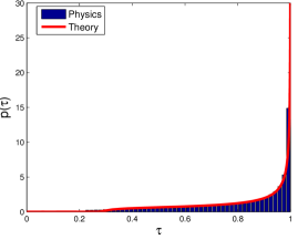
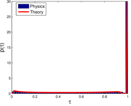
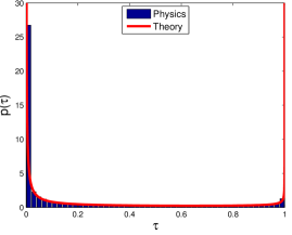
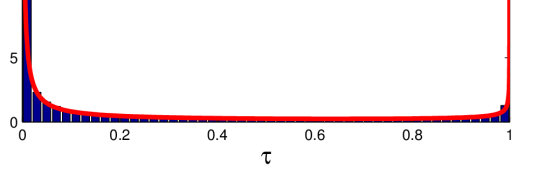
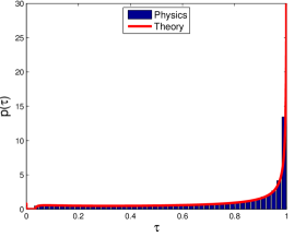
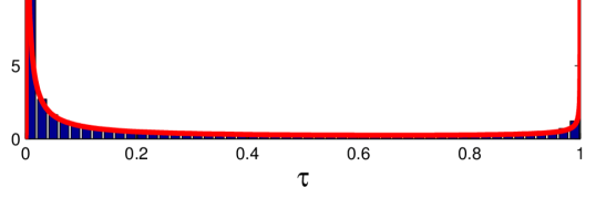
We first consider the setting where all the randomly placed cylinders have the same refractive index. Plugging in into Eq. (29) yields the expression
| (48) |
For , we get and . Plugging in into Eq. (48) and solving Eq. (36) yields the transmission coefficient as a function of . Fig. 3 shows the agreement between the physically rigorous empirical distribution and the analytically predicted distribution. Note in particular, the agreement for where the distribution is far from the characteristically bimodal DMPK distribution.
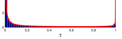
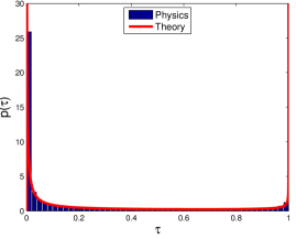
We now consider the setting where with probability a cylinder has refractive index and with probability it has a refractive index . Plugging in into Eq. (29) yields the expression
| (49) |
For and we get , , and , . Plugging in these values into Eq. (49) with and and solving Eq. (36) yields the transmission coefficient as a function of . Fig. 4 shows the agreement between the numerically obtained empirical distribution and the analytically predicted distribution. Note in particular, the agreement for where the predicted distribution is supported on two intervals and agrees with the empirical results.
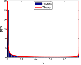
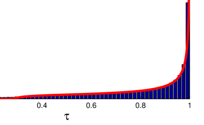
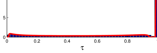
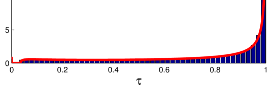
Finally, we consider the setting corresponding to . We generated the scattering system by mapping each random realization of to a random realization of the refractive index. Plugging this choice into Eq. (29) yields the expression
| (50) |
The choice of and corresponds to a refractive index of (with ) and a refractive index (with ). Plugging these values of and into Eq. (50) and solving Eq. (36) yields the transmission coefficient as a function of . Fig. 5 shows the agreement between the physically rigorous empirical distribution and the analytically predicted distribution. Note in particular, the agreement for where the distribution is far from the characteristically bimodal DMPK distribution.
Appendix D contains some movies that shows the evolution of the transmission coefficient distribution with for each of the three scenarios discussed. As expected, for large enough the distribution eventually becomes characteristically bimodal as predicted by the DMPK theory. The behavior for small values of is accurately predicted by our theory.
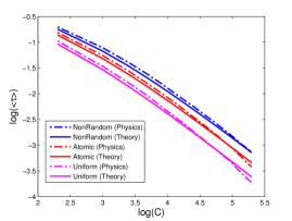
For the three settings described above, we analytically compute from the associated via Eq. (40). The computation involves the normalizing factor , which for the three settings is given by
| (51a) | ||||
| (51b) | ||||
| (51c) | ||||
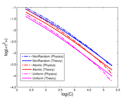
The closed-from expression for is lengthy and therefore omitted here. It can be obtained using the calculations in Appendix C. Fig. 6 compares the empirical moments with the predicted moments and shows the good agreement for a range of values of .
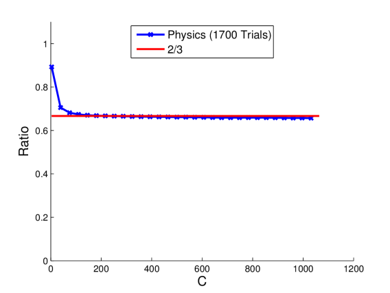
Finally, we numerically validate the analytical prediction in Eq. (46). To that end, we generated a random scattering system with , and . The locations of the scatterers were selected randomly and produced a system with , where is the average distance to the nearest scatterer. Let denote the thickness of the scattering system we are interested in analyzing. We vary from to and for each value of we compute the scattering matrices associated with only the scatterers contained in the portion of the system we have generated. This construction ensures that the average density per “layer” of the medium is about the same. We computed the first and second moment of the empirical transmission coefficient distribution by averaging over random realizations of the scattering system and computed ratio as a function of . Fig. 7 shows that the empirical result validate our theoretical prediction.
Acknowledgements
This work supported by a DARPA Young Faculty Award D14AP00086, AFOSR Young Investigator Award FA9550-12-1-0266, ONR Young Investigator Award N00014-11-1-0660, US Army Research Office (ARO) under grant W911NF-11-1-0391 and NSF grant CCF-1116115.
Appendices
Appendix A Derivation of Eq. (10)
Here, we uncover the relationship between the singular value squared of , , and the singular value squared of , . Our derivation follows the approach in [5, Section 1.C.1].
A.A Decomposition of
Recall that the eigenvalues of equal the square singular values of . Using Eq. (9) and the fact that , we can express as
| (56) | ||||
| (59) |
In order to factorize the matrix on the right-hand side of Eq. (59) further, we first factorize the submatrices of the scattering matrix as
| (60a) | ||||
| (60b) | ||||
| (60c) | ||||
| (60d) | ||||
where and , and represents the phase ambiguity between the singular spaces. Note that the factorizations in Eq. (60) satisfies power conservation, reciprocity and time-reversal symmetry. Substituting these into Eq. (59) yields the factorization
| (63) | ||||
| (70) |
Note that this factorization reveals that the eigenvalues of are exactly equal to the eigenvalues of .
A.B Eigenvalues of a special block matrix
Note that the matrix on the right-hand side of Eq. (63) is of the form
where , , and . The eigenvalues of this block matrix are the solutions of the characteristic equation
Since the eigenvalues will not be the same as , will be invertible; hence the characteristic equation can be rewritten as
Equivalently,
Consequently, the eigenvalues are given by
| (71) |
A.B.1 Relationship between the singular values of and
Recall that is the eigenvalue of and is an eigenvalue of . We can apply Eq. (71) to the matrix in Eq. (70) to obtain the eigenvalues of , which are given by
| (72) | ||||
| (73) |
Note that . This tells us that the singular values of the transfer matrix come in reciprocal pairs. Consequently, if we specify the singular values above one then the singular values below one are given by their reciprocal.
Appendix B Derivation of Eq. (40) for
From Eq. (39) the first moment is given as
In order to evaluate this further, we are going to use what we have driven in Eq. (33),
Using the relationship between and in Eq. (21), we get
| (74) |
Therefore,
| (75) |
where is a value that satisfies or . We can easily check that by plugging it into Eq. (74).
| (76) |
From Eq. (29), we can evaluate as follows
| (77) | ||||
| (78) |
Therefore we confirm
| (79) |
To complete Eq. (75), we need to evaluate . Straightforward evaluation leads to the following result,
| (80) |
and we get
Appendix C Closed-form expression for
For notational convenience we define
| (81a) | ||||
| (81b) | ||||
| (81c) | ||||
| (81d) | ||||
From Eq. (43) we have
| (82) |
As we did for the first moment, we are going to express this in terms of the inverse function of . We are going to use the following elementary results from calculus
| (83a) | ||||
| (83b) | ||||
Appendix D Movies showing evolution of the transmission coefficient distribution with
\animategraphics[controls,buttonsize=0.3cm,width=12.5cm] 10”movies/EvolutionNonRand”1259
\animategraphics[controls,buttonsize=0.3cm,width=12.5cm] 10”movies/EvolutionRand”1259
\animategraphics[controls,buttonsize=0.3cm,width=12.5cm] 10”movies/EvolutionUniform”1259
References
- [1] Greg W Anderson and Brendan Farrell. Asymptotically liberating sequences of random unitary matrices. Advances in Mathematics, 255:381–413, 2014.
- [2] J. Aulbach, B. Gjonaj, P. M. Johnson, A. P. Mosk, and A. Lagendijk. Control of light transmission through opaque scattering media in space and time. Physical review letters, 106(10):103901, 2011.
- [3] C. Barnes and J. B. Pendry. Multiple scattering of waves in random media: a transfer matrix approach. Proceedings of the Royal Society of London. Series A: Mathematical and Physical Sciences, 435(1893):185, 1991.
- [4] C. W. J. Beenakker. Applications of random matrix theory to condensed matter and optical physics. Arxiv preprint arXiv:0904.1432, 2009.
- [5] Carlo WJ Beenakker. Random-matrix theory of quantum transport. Reviews of modern physics, 69(3):731, 1997.
- [6] M. Cui. A high speed wavefront determination method based on spatial frequency modulations for focusing light through random scattering media. Optics Express, 19(4):2989–2995, 2011.
- [7] M. Cui. Parallel wavefront optimization method for focusing light through random scattering media. Optics letters, 36(6):870–872, 2011.
- [8] O. N. Dorokhov. Transmission coefficient and the localization length of an electron in N bound disordered chains. JETP Lett, 36(7), 1982.
- [9] Fumio Hiai and Dénes Petz. The semicircle law, free random variables and entropy, volume 77. American Mathematical Society Providence, 2000.
- [10] R. A. Horn and C. R. Johnson. Matrix analysis. Cambridge university press, 1990.
- [11] A. Ishimaru. Wave propagation and scattering in random media, volume 12. Wiley-IEEE Press, 1999.
- [12] C. Jin, R. R. Nadakuditi, E. Michielssen, and S. Rand. An iterative, backscatter-analysis based algorithm for increasing transmission through a highly-backscattering random medium. In Statistical Signal Processing Workshop (SSP), 2012 IEEE, pages 97–100. IEEE, 2012.
- [13] C. Jin, R. R. Nadakuditi, E. Michielssen, and S. Rand. Iterative, backscatter-analysis algorithms for increasing transmission and focusing light through highly scattering random media. JOSA A, 30(8):1592–1602, 2013.
- [14] M. Kim, Y. Choi, C. Yoon, W. Choi, J. Kim, Q.-Han. Park, and W. Choi. Maximal energy transport through disordered media with the implementation of transmission eigenchannels. Nature Photonics, 6(9):583–587, 2012.
- [15] T. W. Kohlgraf-Owens and A. Dogariu. Transmission matrices of random media: Means for spectral polarimetric measurements. Optics letters, 35(13):2236–2238, 2010.
- [16] R. C. McPhedran, L. C. Botten, A. A. Asatryan, N. A. Nicorovici, P. A. Robinson, and C. M. De Sterke. Calculation of electromagnetic properties of regular and random arrays of metallic and dielectric cylinders. Physical Review E, 60(6):7614, 1999.
- [17] P. A. Mello, P. Pereyra, and N. Kumar. Macroscopic approach to multichannel disordered conductors. Annals of Physics, 181(2):290–317, 1988.
- [18] J. B. Pendry, A. MacKinnon, and A. B. Pretre. Maximal fluctuations–a new phenomenon in disordered systems. Physica A: Statistical Mechanics and its Applications, 168(1):400–407, 1990.
- [19] S. M. Popoff, G. Lerosey, R. Carminati, M. Fink, A. C. Boccara, and S. Gigan. Measuring the transmission matrix in optics: an approach to the study and control of light propagation in disordered media. Physical review letters, 104(10):100601, 2010.
- [20] C. Schwartz. A classical perturbation theory. Journal of Mathematical Physics, 18:110, 1977.
- [21] Z. Shi, J. Wang, and A. Z. Genack. Measuring transmission eigenchannels of wave propagation through random media. In Frontiers in Optics. Optical Society of America, 2010.
- [22] A. Sidi. Practical extrapolation methods, volume 10 of Cambridge Monographs on Applied and Computational Mathematics. Cambridge University Press, Cambridge, 2003.
- [23] S. Singh and R. Singh. On the use of Shank’s transform to accelerate the summation of slowly converging series. Microwave Theory and Techniques, IEEE Transactions on, 39(3):608–610, 1991.
- [24] C. Stockbridge, Y. Lu, J. Moore, S. Hoffman, R. Paxman, K. Toussaint, and T. Bifano. Focusing through dynamic scattering media. Optics Express, 20(14):15086–15092, 2012.
- [25] E. G. van Putten, A. Lagendijk, and A. P. Mosk. Optimal concentration of light in turbid materials. JOSA B, 28(5):1200–1203, 2011.
- [26] I. M. Vellekoop and A. P. Mosk. Phase control algorithms for focusing light through turbid media. Optics Communications, 281(11):3071–3080, 2008.
- [27] I. M. Vellekoop and A. P. Mosk. Universal optimal transmission of light through disordered materials. Physical review letters, 101(12):120601, 2008.
- [28] D. V. Voiculescu, K. J. Dykema, and A. Nica. Free random variables. Number 1. American Mathematical Soc., 1992.
- [29] Dan Voiculescu. Limit laws for random matrices and free products. Inventiones mathematicae, 104(1):201–220, 1991.