Entangled quantum probes for dynamical environmental noise

Abstract

We address the use of entangled qubits as quantum probes to characterize the noise induced by complex environments. In particular, we show that a joint measurement on entangled probes can improve estimation of the correlation time for a broad class of environmental noises compared to any sequential strategy involving single qubit preparation. The enhancement appears when the noise is faster than a threshold value, a regime which may always be achieved by tuning the coupling between the quantum probe and the environment inducing the noise. Our scheme exploits time-dependent sensitivity of quantum systems to decoherence and does not require dynamical control on the probes. We derive the optimal interaction time and the optimal probe preparation, showing that it corresponds to multiqubit GHZ states when entanglement is useful. We also show robustness of the scheme against depolarization or dephasing of the probe, and discuss simple measurements approaching optimal precision.

The coherence properties of a quantum system are strongly affected by its interaction with the surrounding environment. This is often an obstacle to the implementation of quantum technologies, so that much effort has been devoted to study the system-environment interaction and to engineer decoherence in order to minimize its degrading effects Davies (1976); Breuer and Petruccione (2007). On the other hand, the very sensitivity of quantum systems to external influence also provides an effective tool to characterize unknown parameters of a given environment Escher et al. (2011); Alipour et al. (2014) by exploiting quantum probes, as opposed to classical ones, usually macroscopic and more intrusive. Indeed, characterizing the noise induced by an external complex system is of great relevance in many areas of nanotechnology, as well as in monitoring biological or chemical processes Hänggi and Jung (1995); Taylor et al. (2008); Mittermaier and Kay (2009); Zhong and Xin (2001). Besides, it represents a crucial step to design robust quantum protocols resilient to noise Bylander et al. (2011); Zhang et al. (2007); Ali Ahmed et al. (2013); Almog et al. (2011); Banchi et al. (2014); Vasile et al. (2014).

The proper framework to address characterization by quantum probes Chin et al. (2012); Haikka and Maniscalco (2014), and to design the best working conditions, is given by quantum estimation theory Paris (2009), which provides analytical tools to optimize the three building blocks of an estimation strategy: (i) preparation of the probe system in a suitably optimized state, (ii) controlled interaction of the probe with the system for an optimal amount of time $t$, (iii) measurement of an optimal observable on the probe. Overall, the ultimate precision for any unbiased estimator $\hat{\gamma}$ of a certain parameter $\gamma$ is bounded by the quantum Cramèr-Rao (CR) theorem, stating that $\text{Var}(\hat{\gamma})\geq[MH(\gamma)]^{-1}$, where $M$ is the number of measurements and $H(\gamma)$ is the quantum Fisher information (QFI), i.e. the superior of the Fisher information over all possible quantum measurements described by positive operator-valued measures (POVMs).

Recently, single-qubit quantum probes have been proposed for the characterization of noise by monitoring decoherence and dephasing induced by the environment under investigation, in particular when the latter can be described in terms of classical stochastic processes Álvarez and Suter (2011); Paris (2014); Benedetti et al. (2014a); Cywiński (2014); Benedetti and Paris (2014). Indeed, stochastic modeling of the environment has been proven Crow and Joynt (2014) to reliably describe noise and the decoherence process in several systems affected by dephasing Neder et al. (2011); Biercuk and Bluhm (2011); Witzel et al. (2014); Fink and Bluhm (2014); Yu and Eberly (2010); Li and Liang (2011); Benedetti et al. (2013, 2012). It may also be useful for several other systems of interest, including motional averaging Li et al. (2013) and solid state qubits Burkard (2009); Wold et al. (2012); Benedetti et al. (2014b).

In this paper, we extend this analysis to entangled qubits used as quantum probes, and show how they greatly improve the characterization of a broad class of environmental noises compared to any sequential strategy involving single qubit preparation D’Ariano et al. (2001); Fujiwara (2001); Acín et al. (2001). In particular, we show how to improve estimation of the correlation time (i.e. the spectral width) of classical noise. Since such noise is usually emerging from a large collection of fluctuators, we are going to consider Gaussian stochastic processes.

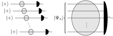
Figure 1: Schematic diagram of possible characterization techniques. On the left: we have $N$ qubits and each one is prepared in the state $\ket{+}$, then interacts with the system for a time $t$ and is finally measured independently of the other qubits. On the right: the $N$ qubits are initially prepared in a multiqubit GHZ state $\ket{\Psi_{\text{\tiny N}}}$, and are let interact with the system such that they are subject to the same realization of the noise. At the output, a collective measurement is performed on the qubits.

The probing scheme is depicted in Fig. 1, both for a sequence of $N$ uncorrelated qubits and for an $N$-qubit entangled state. In both cases we assume that the qubits do not interact with each other. In each case, the qubits may interact with different realizations of the noise or with the same realization, depending on the temporal and spatial distance between the probes. We end up with four possible schemes, which we describe in detail in the Appendix. In the following, we focus on the best case for each configuration, i.e. independent realizations for the separable probes and a common environment for entangled probes.

Let us start by considering a single qubit interacting with a fluctuating dephasing environment. The Hamiltonian is given by $\mathcal{H}(t)=\omega_{0}\sigma_{z}+B(t)\sigma_{z},$ where $\omega_{0}$ is the energy of the qubit and $B(t)$ is a realization of the stochastic process that describes the noise. As a paradigmatic example we consider a zero-mean Ornstein-Uhlenbeck process characterized by the autocorrelation function $K(t,t^{\prime})\equiv\braket{B(t)B(t^{\prime})}_{B}=\frac{1}{2}\gamma\Gamma\exp[-\gamma|t-t^{\prime}|]$, or by the corresponding Lorentzian spectrum. Here, $\gamma$ is the spectral width, i.e. the inverse of the autocorrelation time, while $\Gamma$ denotes the coupling between the probe and the system. It is worth noticing that a similar analysis may be carried out for other Gaussian processes, e.g. processes with power-law or Gaussian autocorrelation functions, and that results are qualitatively the same, independently on the choice of the autocorrelation function.

The density operator of the evolved qubit is given by

$$\rho(t)=\braket{U(t)\rho(0)U^{\dagger}(t)}_{B},$$ (1)

where $\braket{\cdot}_{B}$ denotes the average over all possible realizations of the stochastic process in the time interval $[0,t]$, $U(t)=\exp[-i\int_{0}^{t}\mathcal{H}(s)ds]=\exp\{[-i\omega_{0}t+\phi(t)]\sigma_{z}\}$ is the time evolution operator, and $\phi(t)=\int_{0}^{t}B(s)ds$ is the accumulated phase due to the environmental (dynamical) noise. An explicit expression for $\rho(t)$ can be found by employing the characteristic function of a zero-mean Gaussian stochastic process: $\left\langle e^{im\phi(t)}\right\rangle=e^{-\frac{1}{2}m^{2}\beta_{\gamma}(t)},$ where

$$\beta_{\gamma}(t)=\int_{0}^{t}\int_{0}^{t}ds\,dw\,K(s,w)=\frac{\Gamma}{\gamma}(e^{-\gamma t}+\gamma t-1).$$ (2)

If the qubit is initially prepared in a state described by the density operator $\rho(0)$, the density operator at the time $t$ will be $\rho(t)$ with $\rho_{kk}(t)=\rho_{kk}(0)$, $k=1,2$ and

$$\rho_{12}(t)=e^{-2\left[i\omega_{0}t+\beta_{\gamma}(t)\right]}\,\rho_{12}(0)\,.$$ (3)

The optimal single qubit preparation, given by $|+\rangle=\frac{1}{\sqrt{2}}(|0\rangle+|1\rangle)$, together with the corresponding QFI and the optimal measurement for the estimation of $\gamma$ have recently been found Benedetti and Paris (2014). For $N$ uncorrelated qubits, thanks to additivity, the QFI is just $N$ times the single qubit QFI, i.e.

$$H_{\text{\tiny N}}^{\text{\tiny{SEP}}}(\gamma,t)=\frac{4N}{e^{4\beta_{\gamma}(t)}-1}[\partial_{\gamma}\beta_{\gamma}(t)]^{2}.$$ (4)

Let us now consider a probe made of $N$ qubits initially prepared in the generalized GHZ entangled state $\ket{\Psi_{\text{\tiny N}}}=(\ket{0}^{\otimes N}+\ket{1}^{\otimes N})/\sqrt{2}\,$, interacting with a common environment.The overall Hamiltonian is thus

$$\mathcal{H}^{(\text{\tiny N})}(t)=\mathcal{H}(t)\otimes\mathbb{I}^{\otimes N-1}+\mathbb{I}\otimes\mathcal{H}(t)\otimes\mathbb{I}^{\otimes N-2}+\ldots,$$ (5)

where $\mathcal{H}(t)$ is the above single qubit Hamiltonian and $B(t)$ is the same realization of the noise for all the qubits. The QFI for the parameter $\gamma$ reads

$$H_{\text{\tiny N}}^{\text{\tiny{GHZ}}}(\gamma,t)=\frac{4N^{4}}{e^{4N^{2}\beta(t,\gamma)}-1}[\partial_{\gamma}\beta_{\gamma}(t)]^{2}\,.$$ (6)

We notice that $\beta_{\gamma}(t)$ is a monotonically increasing function of $t$ with $\beta_{\gamma}(0)=0$ (see Eq. (2)). Moreover, we have $\beta_{\gamma}(t)\sim\Gamma(t-1/\gamma)$ for $t\gg 1$. Thus both $H_{\text{\tiny N}}^{\text{\tiny{SEP}}}(\gamma,t)$ and $H_{\text{\tiny N}}^{\text{\tiny{GHZ}}}(\gamma,t)$ are asymptotically vanishing and show a single maximum, corresponding to different optimal values of the interaction time, $t_{\text{opt}}^{\text{\tiny{SEP}}}$ and $t_{\text{opt}}^{\text{\tiny{GHZ}}}$ respectively. We refer to this maximum value as the maximal QFI for a specific value of $\gamma$. As is apparent from the above equations, the maximization of the QFI involves transcendental equations and must be done numerically. The behavior of $H_{\text{\tiny N}}^{\text{\tiny{SEP}}}(\gamma,t)$ and $H_{\text{\tiny N}}^{\text{\tiny{GHZ}}}(\gamma,t)$ is depicted in the upper left panel of Fig. 2. The lower panels of the figure show how the optimal time depends on $\gamma$ for the two measurement schemes.

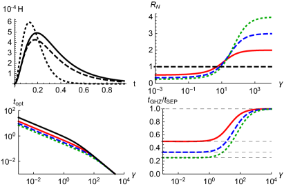
Figure 2: (Color online) In the upper left panel, the QFI $H_{2}^{\text{\tiny{SEP}}}(t)$ (solid) and $H_{2}^{\text{\tiny{GHZ}}}(t)$ (dotted) as function of time for $\gamma=10$. We also show for comparison the (smaller) QFI for separable two-qubit probes in a common environment (dashed) . In the upper right the QFI ratio $\text{R}_{\text{\tiny N}}$ as a function of $\gamma$ (log scale) for $N=2$ (solid red), $N=3$ (dashed blue) and $N=4$ (dotted green). For small values of $\gamma$, the ratio is below one (black dashed line), and tends asymptotically to $1/N$: in this regime it is more convenient to employ separable states than maximally entangled states. The ratio increases monotonically with $\gamma$ and exceeds one at a threshold value $\gamma_{0}(N)$, which depends on $N$. For asymptotically large $\gamma$, the use of $N$-qubit GHZ states is $N$ times better than the use of $N$ qubits in a separable state. In the lower left pannel, a log-log plot of the optimal interaction time as a function of $\gamma$ for separable probes (black), and for an entangled probe with $2$ (solid red), $3$ (dashed blue) and $4$ (dotted green) qubits. In the lower right panel, the ratio between the optimal time for the GHZ state, $t_{\text{\tiny{GHZ}}}$ and for the separable state $t_{\text{\tiny{SEP}}}$.

In situations where we can control the interaction time between the probe and the environment, it will be most convenient to set it to the optimal time. Thus, a fair comparison between separable and entangled probes naturally involves the maximal QFI of the two cases. We therefore introduce the QFI ratio as $\text{R}_{\text{\tiny N}}(\gamma)={H^{\text{\tiny{GHZ}}}_{\text{\tiny N},\text{\tiny max}}(\gamma)}/{H^{\text{\tiny{SEP}}}_{\text{\tiny N},\text{\tiny max}}(\gamma)}\,$, and analyze its behavior as a function of $\gamma$ and N. When $\text{R}_{\text{\tiny N}}(\gamma)>1$, the use of a $N$ qubits in a GHZ state improves estimation compared to the use of $N$ uncorrelated probes, e.g. in a sequential strategy. Figure 2 illustrates the main results: the ratio $\text{R}_{\text{\tiny N}}(\gamma)$ is larger than one for $\gamma>\gamma_{0}(N)$, where $\gamma_{0}(N)$ is a threshold value that depends on $N$. Moreover, $\text{R}_{\text{\tiny N}}(\gamma)\rightarrow N$ for $\gamma\gg\gamma_{0}(N)$. This result is enhanced by the fact that, upon substituting $\tilde{\gamma}=\gamma/\Gamma$ and $\tau=\tilde{\gamma}t$, we may show that the quantum signal-to-noise ratio (QSNR) $\tilde{\gamma}^{2}H(\tilde{\gamma})$ does not depend on $\Gamma$. This means that, if one is able to control the coupling between the probe and the system, one can always tune $\Gamma$ to achieve a situation where $\text{R}_{\text{\tiny N}}(\tilde{\gamma})>1$. All the Figures are obtained by setting $\Gamma=1$.

Now a question arises: Is the GHZ state $\ket{\Psi_{\text{\tiny N}}}$ the optimal one? Are there (entangled) states that give even higher QFI? The answer to this question cannot be analytic, because one cannot diagonalize analytically a generic density matrix of a multiqubit state. In order to attack this problem, we first notice that the maximum is achieved for an initial pure state Fujiwara (2001). We have thus generated a large number ($n=10^{6}$) of random initial pure states, uniformly distributed according to the Haar measure, for different values of $\gamma$ and for $N=2,3,4$. For each random state, the maximal QFI, $H^{\text{\tiny{RND}}}_{\text{\tiny N}}(\gamma)$, resulting from the interaction with a common environment has been numerically evaluated using the expression $H(\gamma)=2\sum_{nm}{|\braket{\psi_{m}}{\partial_{\gamma}\rho_{\gamma}}{\psi_{n}}|^{2}}/(\rho_{n}+\rho_{m}),$ where $\rho_{\gamma}=\sum_{n}\rho_{n}\ket{\psi_{n}}\bra{\psi_{n}}$ is the diagonal form of the density operator after the interaction with the environment. This value is then used to evaluate the corresponding QFI ratio $H^{\text{\tiny{RND}}}_{\text{\tiny N}}(\gamma)/H^{\text{\tiny{SEP}}}_{\text{\tiny N}}(\gamma)$, and to compare the estimation precision to the precision achievable using $N$ independent qubits interacting with separate environments. Our results indicate that, for $\gamma\gtrsim\gamma_{0}$, that is, in the region where entanglement is convenient, the GHZ state is indeed the optimal one, thus showing that entanglement is a resource for the estimation of the spectral width of Gaussian noise.

Below the threshold the GHZ state interacting with a common environment is no longer optimal and the optimal strategy involves separable probes interacting with independent environments. For completeness, we anyway look for the optimal state in a common environment and found numerically that the extremal state lies in the same family of states that had been identified in Huelga et al. (1997) as optimal probes to improve frequency estimation. The states of this family, for $N$ qubits, have the form $\ket{\Phi_{\text{\tiny N}}}=\sum_{k=0}^{\lfloor\frac{1}{2}\text{\tiny N}\rfloor}a_{k}\ket{k},$ where $a_{k}$ are normalized real coefficients, $\ket{k}$ is an equally weighted superposition of all $N$-qubit states with a number $k$ or a number $N-k$ of excitations, and $\lfloor\cdot\rfloor$ denotes the integer part. The GHZ state belongs to this family with $a_{0}=1/\sqrt{2}$ and all other coefficients set to $0$.

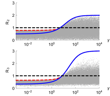
Figure 3: (Color online) The curves in the logplots show the QFI ratio $\text{R}_{2}$ (top) and $\text{R}_{3}$ (bottom) as a function of $\gamma$ for the GHZ state (solid blue) and the optimal state of $N$ qubits in a common environment (dashed red). The two curves superimpose each other above the threshold $\gamma_{0}(N)$. We also show the QFI ratio for $10^{5}$ randomly generated states (gray points), uniformly distributed according to the Haar measure.

Figure 3 illustrates our numerical results obtained for two and three qubits. The plots show the QFI ratios $\text{R}_{2}$ (left) and $\text{R}_{3}$ (right). The solid blue line is the ratio for the GHZ state, the $10^{4}$ gray points correspond to the QFI ratio of randomly generated states and the dashed red line is found by optimizing the QFI over the coefficients $a_{k}$ of $\ket{\Phi_{\text{\tiny N}}}$. We can see that from $\gamma\gtrsim\gamma_{0}(N)$ the blue and red curves coincide, i.e. GHZ states are extremal. We also notice that for $\gamma\gtrsim\gamma_{0}(N)$ a significant fraction of gray dots lies above the $r=1$ dashed line, but the dots are sparse around the solid blue line, meaning that the GHZ state allows for a remarkable gain in the estimation of larger values of $\gamma$.

It is worth to emphasize that optimal precision, i.e. the QFI of Eq. (6) may be achieved upon implementing a simple rank-2 measurement. Indeed, $H_{\text{\tiny N}}^{\text{\tiny{GHZ}}}(\gamma)$ corresponds to the Fisher information of a projective measurement on the two eigenvectors corresponding to the nonzero eigenvalues of the evolved density operator, which are, respectively

$$p_{\pm} =\frac{1}{2}\left(1\pm e^{-2N^{2}\lambda^{2}\beta_{\gamma}(t)}\right)$$ (7)

$$\ket{p_{\pm}} =\frac{1}{\sqrt{2}}(e^{-i\omega_{0}\sigma_{z}})^{\otimes N}\left(\ket{0}^{\otimes N}\pm\ket{1}^{\otimes N}\right).$$ (8)

The CR theorem, however, sets only a lower bound to the precision of any unbiased estimator, and a question arises on how to suitably process data coming from the above rank-2 measurement in order to saturate the bound. Bayesian estimators are known to saturate the CR bound for asymptotically large numbers of measurements: in order to assess quantitatively the performance of Bayesian estimation we have performed simulated experiments on the probing system. In particular, we have simulated the outcomes $\{x_{1},\ldots,x_{M}\}$ of the measurement by randomly choosing a result according to the probabilities of Eq. (7) and have built a Bayesian estimator $\hat{\gamma}$ as the mean value of the a posteriori distribution, starting from a flat prior. The resulting relative error of $\hat{\gamma}$, $\epsilon=\sqrt{\text{Var}(\hat{\gamma})}/\hat{\gamma}$, is shown, as a function of the number of measurements, in Fig. 4 for a specific value of $\gamma$. We see that with a relatively low number of measurements, of the order of thousands, the bound is saturated and the situation improves by increasing the number of qubits. The proposed scheme thus allows for an effective and achievable estimation of the parameter $\gamma$.

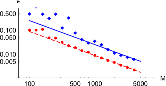
Figure 4: (Color online) Log-log plot of the relative error $\epsilon=\sqrt{\text{Var}(\hat{\gamma})}/\hat{\gamma}$ of the Bayesian estimator as a function of the number of measurements, for $\gamma=10$. The lines represent the CR bound for a single-qubit measurement (dashed blue) and for a 4-qubit GHZ state (solid red). The diamonds (single qubit) and the dots (4 qubits) correspond to the performance of a Bayes estimator applied to simulated experiments. Bayes estimators saturate the CR bound when increasing the number of measurements and very good performances are achieved already for thousands of measurements. The plot also shows that estimation improves with the number of qubits since the CR bound is saturated with a lower number of measurement.

Let us now address the robustness of our scheme against noise in the preparation of the probe. In fact, we have shown that the use of entangled qubit probes prepared in a GHZ state leads to enhanced precision in the estimation of the spectral width. However, it is generally challenging to experimentally prepare the probes exactly in the GHZ state and a question arises on how sensible is this estimation scheme to, e.g., the purity of the initial preparation. We answer this question by considering a partially depolarized state, $\rho_{p}=p\,\rho_{\text{\tiny{GHZ}}}+(1-p)\mathbb{I}/2^{N}$, where $\mathbb{I}$ is the identity matrix and $0<p<1$, and a partially dephased state, $\rho_{\delta}=\delta\rho_{\text{\tiny{GHZ}}}+\frac{1}{2}(1-\delta)(\ket{0}^{\otimes N}\bra{0}+\ket{1}^{\otimes N}\bra{1})$ where $0<\delta<1$. In both cases, an analytic expression for the QFI may be found: we have

$$H^{p}_{\text{\tiny N}}(\gamma,t) =\frac{2^{N+2}N^{4}\left[\left(2^{N}-2\right)p+2\right]p^{2}[\partial_{\gamma}\beta_{\gamma}(t)]^{2}}{\left[\left(2^{N}-2\right)p+2\right]^{2}e^{4N^{2}\beta(t,\gamma)}-4^{N}p^{2}}$$ (9)

$$H_{\text{\tiny N}}^{\delta}(\gamma,t) =\frac{4N^{4}\delta^{2}}{e^{4N^{2}\beta(t,\gamma)}-\delta^{2}}[\partial_{\gamma}\beta_{\gamma}(t)]^{2}\,,$$ (10)

which are obviously less than $H^{\text{\tiny{GHZ}}}_{\text{\tiny N}}(\gamma)$, being $\rho_{p}$ and $\rho_{\delta}$ mixed states, but may be still larger than $H_{\text{\tiny N}}^{\text{\tiny{SEP}}}(\gamma)$. Indeed, Figure 5 shows that for each value of $\gamma$ above $\gamma_{0}(N)$ there is a threshold value for the purity, above which the use of a depolarized or dephased GHZ state still leads to an improvement over the use of $N$ uncorrelated probes. The threshold purity $\mu_{0}$ is close to one for $\gamma\simeq\gamma_{0}(N)$ and for $\gamma\gg\gamma_{0}(N)$, whereas it shows a minimum in the intermediate region, thus allowing for a certain tolerance in the preparation of the initial state of the probe. Besides, this minimum value of the threshold gets lower when increasing the number of qubits.

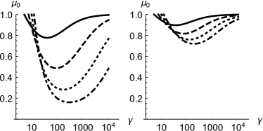
Figure 5: Threshold purity $\mu_{0}$, as a function of the spectral width $\gamma$, above which the use of a depolarized (left panel) or a dephased GHZ state (right panel) is more effective than a set of uncorrelated qubits. The different lines correspond to a different number $N$ of qubits: $N=2$ (solid), $N=3$ (dashed), $N=4$ (dotted), $N=5$ (dot-dashed). The threshold $\mu_{0}$ approaches 1 when $\gamma\rightarrow\gamma_{0}(N)$ and when $\gamma\rightarrow\infty$, whereas there is an intermediate region where $\mu_{0}$ decreases to a minimum, meaning that there is more tolerance in the initial preparation of the probe. When $N$ increases the minimum of $\mu_{0}$ decreases and moves to larger values of $\gamma$.

In conclusion, we have shown that the use of entangled qubits as quantum probes outperforms the sequential use of single-qubit probes in the characterization of the noise induced by complex environments. In particular, we have shown that a joint measurement on entangled probes improves estimation of the correlation time for a broad class of environmental noises when the noise is faster than a threshold value. This result is enhanced by the fact that, upon controlling the coupling between the probe and the system, the threshold value can be reduced arbitrarily. Our scheme exploits time-dependent sensitivity of quantum systems to decoherence and does not require dynamical control on the probes. We have found the optimal interaction time and the optimal multiqubit probe preparation, showing that it corresponds to multiqubit GHZ states. The proposed measurement scheme achieves the Cramér-Rao bound for a relatively low number of measurements, upon employing a Bayesian estimator, and is robust against imperfect preparation of the initial entangled state.

Appendix A Supplemental Material

We consider probes prepared both in the separable state $\ket{+}^{\otimes N}$ and in the generalized GHZ entangled state $\ket{\Psi_{\text{\tiny N}}}=(\ket{0}^{\otimes N}+\ket{1}^{\otimes N})/\sqrt{2}\,$.

We also consider two possible scenarios: in the first, each qubits interacts with an independent realization of the noise. This means that the overall Hamiltonian is

$$\mathcal{H}^{(\text{\tiny N})}(t)=\mathcal{H}_{1}(t)\otimes\mathbb{I}^{\otimes N-1}+\mathbb{I}\otimes\mathcal{H}_{2}(t)\otimes\mathbb{I}^{\otimes N-2}+\ldots,$$ (11)

where the realizations of the stochastic processes in each Hamiltonian $\mathcal{H}_{i}(t)$ are uncorrelated, and the expected value of Eq. (2) must be calculated over all possible realizations of $B_{1}(t),\ldots,B_{N}(t)$. In the second scenario all the qubits interact with a common environment and the qubits interact with the same realization of the noise. Then $\mathcal{H}_{1}(t)=\ldots=\mathcal{H}_{N}(t)=\mathcal{H}(t)$ and the expected value in Eq. (2) must be calculated over all possible realizations of a single stochastic process $B(t)$.

We now show the results involving all the four possible probing schemes and show that a probing scheme involving $N$ qubits initially prepared in a GHZ state and interacting with a common environment outperforms any probing scheme involving $N$ qubits in the separable state $\ket{+}^{\otimes N}$ when $\gamma$ is greater than a threshold value.

A.1 Separable probes, independent enviroments

Since each qubit interacts with an independent realization of the noise, this scheme amounts to $N$ repetitions of the measurement of a single qubit probe prepared in the optimal state, Eq. (24) of Ref. Benedetti and Paris (2014), and thus, thanks to the additivity of the QFI,

$$H_{\text{\tiny N}}^{\text{\tiny{SEP}},\text{\tiny{IE}}}(\gamma,t)=\frac{4N}{e^{4\beta_{\gamma}(t)}-1}[\partial_{\gamma}\beta_{\gamma}(t)]^{2}.$$ (12)

A.2 Separable probes, common environment

In this scenario the dynamics of each qubits is not independent and we need to determine the dynamics of the whole $N$-qubit state. The QFI has a readable analytical form only for two qubits

$$H_{2}^{\text{\tiny{SEP}},\text{\tiny{CE}}}(\gamma,t)=\frac{32\left\{e^{8\beta_{\gamma}(t)}[\sinh 4\beta_{\gamma}(t)+1]+1\right\}}{3e^{16\beta_{\gamma}(t)}-2e^{8\beta_{\gamma}(t)}+1}[\partial_{\gamma}\beta_{\gamma}(t)]^{2}.$$ (13)

One can easily see that

$$\forall t,\gamma\qquad H_{2}^{\text{\tiny{SEP}},\text{\tiny{IE}}}(\gamma,t)>H_{2}^{\text{\tiny{SEP}},\text{\tiny{CE}}}(\gamma,t),$$ (14)

since $\beta_{\gamma}(t)>0$.

We checked numerically that the maximal QFI for separable probes interacting with a common environment is always lower to the maximal QFI for separable probes interacting with independent environments for fixed $\gamma$ also for $N=3$ and $N=4$. The results, shown in Fig. 6, indicate that the ratio between $H_{n}^{\text{\tiny{SEP}},\text{\tiny{CE}}}(\gamma,t)$ and $H_{2}^{\text{\tiny{SEP}},\text{\tiny{IE}}}(\gamma,t)$ decreases with $N$.

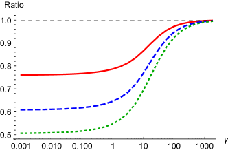
Figure 6: Ratio between $H_{\text{\tiny N}}^{\text{\tiny{SEP}},\text{\tiny{CE}}}(\gamma,t)$ and $H_{\text{\tiny N}}^{\text{\tiny{SEP}},\text{\tiny{IE}}}(\gamma,t)$ for $N=2$ (solid red), $N=3$ (dashed blue), $N=4$ (dotted green). The ratio is always lower than one and gets lower as $N$ increases. In the limit $\gamma\gg 1$ the ratio reaches one.

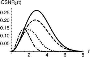
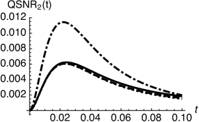
Figure 7: The two plots show the two-qubit quantum signal-to-noise ratio (QSNR) $\gamma^{2}H(\gamma,t)$ as a function of time for two values of the spectral width $\gamma$ of the noise: on the left $\gamma=0.1$ and on the right $\gamma=100$. The solid line shows $\gamma^{2}H_{\text{\tiny N}}^{\text{\tiny{SEP}},\text{\tiny{IE}}}(\gamma,t)$, the dashed line $\gamma^{2}H_{\text{\tiny N}}^{\text{\tiny{SEP}},\text{\tiny{CE}}}(\gamma,t)$, the dotted line $\gamma^{2}H_{\text{\tiny N}}^{\text{\tiny{GHZ}},\text{\tiny{IE}}}(\gamma,t)$ and the dot-dashed line $\gamma^{2}H_{\text{\tiny N}}^{\text{\tiny{GHZ}},\text{\tiny{CE}}}(\gamma,t)$. From the left panel we can see that $H_{\text{\tiny N}}^{\text{\tiny{SEP}},\text{\tiny{IE}}}(\gamma,t)>H_{\text{\tiny N}}^{\text{\tiny{SEP}},\text{\tiny{CE}}}(\gamma,t)$ for all $t$ and that $H_{\text{\tiny N},\max}^{\text{\tiny{GHZ}},\text{\tiny{CE}}}(0.1)>H_{\text{\tiny N},\max}^{\text{\tiny{GHZ}},\text{\tiny{IE}}}(0.1)$. From the right panel we can see that for high values of $\gamma$ the GHZ probes interacting with a common environment outperforms the other schemes.

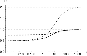
Figure 8: Ratios between $H_{2,\max}^{\text{\tiny{SEP}},\text{\tiny{CE}}}(\gamma)$ (dashed), $H_{2,\max}^{\text{\tiny{GHZ}},\text{\tiny{IE}}}(\gamma)$ (dotted) $H_{2,\max}^{\text{\tiny{GHZ}},\text{\tiny{CE}}}(\gamma)$ (dot-dashed) and $H_{2,\max}^{\text{\tiny{SEP}},\text{\tiny{IE}}}(\gamma)$ as functions of $\gamma$. We can see that the GHZ probes interacting with common environment achieves a higher maximal QFI than the other schemes. Similar plots can be produced for $N>2$.

A.3 GHZ probes, independent environments

In this case, the expected value of the density operator at time $t$ over al possible realizations of the stochastic processes $B_{1}(t),\ldots,B_{N}(t)$, is

$$\begin{split}\rho_{\text{\tiny{GHZ}}}(t)=&\frac{1}{2}(\ket{0\ldots 0}\bra{0\ldots 0}+\ket{1\ldots 1}\bra{1\ldots 1})+\\ &\frac{1}{2}e^{-2N\beta_{\gamma}(t)}(e^{-2iN\omega_{0}}\ket{0\ldots 0}\bra{1\ldots 1}+\text{h.c.})\end{split}$$ (15)

and we find, for the QFI,

$$H_{\text{\tiny N}}^{\text{\tiny{GHZ}},\text{\tiny{IE}}}(\gamma,t)=\frac{4N^{2}}{e^{4N\beta_{\gamma}(t)}-1}[\partial_{\gamma}\beta_{\gamma}(t)]^{2}.$$ (16)

It is quite easy to prove that $H_{\text{\tiny N}}^{\text{\tiny{GHZ}},\text{\tiny{IE}}}(\gamma,t)<H_{\text{\tiny N}}^{\text{\tiny{SEP}},\text{\tiny{IE}}}(\gamma,t)$ for all $t$ and $\gamma$ and so we don’t have an improvement in the estimation of $\gamma$ with a probe in the GHZ state if each qubit interacts with an independent realization of the environment.

A.4 GHZ probes, common environment

If the entangled qubits of the probe are affected by the same realization of the noise one finds that the expected value of $\rho(t)$ is

$$\begin{split}\rho_{\text{\tiny{GHZ}}}(t)=&\frac{1}{2}(\ket{0\ldots 0}\bra{0\ldots 0}+\ket{1\ldots 1}\bra{1\ldots 1})+\\ &\frac{1}{2}(e^{-2Ni\omega_{0}-2N^{2}\beta_{\gamma}(t)}\ket{0\ldots 0}\bra{1\ldots 1}+\text{h.c.})\end{split}$$

and obtains the following expression for the QFI:

$$H_{\text{\tiny N}}^{\text{\tiny{GHZ}},\text{\tiny{CE}}}(\gamma,t)=\frac{4N^{4}}{e^{4N^{2}\beta(t,\gamma)}-1}[\partial_{\gamma}\beta_{\gamma}(t)]^{2}.$$ (17)

A.5 Maximal QFI values

We have shown the analytical equations for the four measurement schemes. Figure 7 shows the dependence on time of the QFI in the four cases and for two values of $\gamma$, which are respectively well below and well above the threshold value $\gamma_{0}$.

We can see that the QFI as a function of time has one maximum. The position of the maximum may not be found analytically, due to the transcendental nature of the optimization equations, but can be found numerically with arbitrary precision.

In Fig. 8 we show the ratios between the maximal values of the QFI for the various cases and the maximal value for the QFI for separable probes interacting with an independent environment, as functions of $\gamma$, in the two-qubit case. We can see that the the ratios are below one except for the scheme involving a joint measurement on entalged probes that interact with a common environment, when $\gamma>\gamma_{0}$. Analogous plots may be produced for $N>2$.

References

- Davies (1976) E. B. Davies, Quantum theory of open systems (Academic Press, 1976).
- Breuer and Petruccione (2007) H.-P. Breuer and F. Petruccione, The Theory of Open Quantum Systems (Oxford University Press, 2007).
- Escher et al. (2011) B. M. Escher, R. L. de Matos Filho, and L. Davidovich, Nat. Phys. 7, 406 (2011).
- Alipour et al. (2014) S. Alipour, M. Mehboudi, and A. Rezakhani, Phys. Rev. Lett. 112, 120405 (2014).
- Hänggi and Jung (1995) P. Hänggi and P. Jung, in Adv. Chem. Phys., Vol. 89, edited by I. Prigogine and S. A. Rice (John Wiley & Sons, Inc., 1995) pp. 239–326.
- Taylor et al. (2008) J. M. Taylor, P. Cappellaro, L. Childress, L. Jiang, D. Budker, P. R. Hemmer, A. Yacoby, R. Walsworth, and M. D. Lukin, Nat. Phys. 4, 810 (2008), arXiv:0805.1367 .
- Mittermaier and Kay (2009) A. K. Mittermaier and L. E. Kay, Trends Biochem. Sci. 34, 601 (2009).
- Zhong and Xin (2001) S. Zhong and H. Xin, Chem. Phys. Lett. 333, 133 (2001).
- Bylander et al. (2011) J. Bylander, S. Gustavsson, F. Yan, F. Yoshihara, K. Harrabi, G. Fitch, D. G. Cory, Y. Nakamura, J.-S. Tsai, and W. D. Oliver, Nat. Phys. 7, 565 (2011).
- Zhang et al. (2007) J. Zhang, X. Peng, N. Rajendran, and D. Suter, Phys. Rev. A 75, 042314 (2007).
- Ali Ahmed et al. (2013) M. Ali Ahmed, G. Álvarez, and D. Suter, Phys. Rev. A 87, 042309 (2013).
- Almog et al. (2011) I. Almog, Y. Sagi, G. Gordon, G. Bensky, G. Kurizki, and N. Davidson, J. Phys. B 44, 154006 (2011).
- Banchi et al. (2014) L. Banchi, P. Giorda, and P. Zanardi, Phys. Rev. E 89, 022102 (2014).
- Vasile et al. (2014) R. Vasile, F. Galve, and R. Zambrini, Phys. Rev. A 89, 022109 (2014).
- Chin et al. (2012) A. W. Chin, S. F. Huelga, and M. B. Plenio, Phys. Rev. Lett. 109, 233601 (2012).
- Haikka and Maniscalco (2014) P. Haikka and S. Maniscalco, Open Syst. Inf. Dyn. 21, 1440005 (2014).
- Paris (2009) M. G. A. Paris, Int. J. Quantum Inf. 7, 125 (2009).
- Álvarez and Suter (2011) G. A. Álvarez and D. Suter, Phys. Rev. Lett. 107, 230501 (2011).
- Paris (2014) M. G. A. Paris, Phys. A Stat. Mech. its Appl. 413, 256 (2014).
- Benedetti et al. (2014a) C. Benedetti, F. Buscemi, P. Bordone, and M. G. A. Paris, Phys. Rev. A 89, 032114 (2014a).
- Cywiński (2014) L. Cywiński, Phys. Rev. A 90, 042307 (2014).
- Benedetti and Paris (2014) C. Benedetti and M. G. A. Paris, Phys. Lett. A 378, 2495 (2014).
- Crow and Joynt (2014) D. Crow and R. Joynt, Phys. Rev. A 89, 042123 (2014).
- Neder et al. (2011) I. Neder, M. S. Rudner, H. Bluhm, S. Foletti, B. I. Halperin, and A. Yacoby, Phys. Rev. B 84, 035441 (2011), arXiv:1103.4862 .
- Biercuk and Bluhm (2011) M. J. Biercuk and H. Bluhm, Phys. Rev. B 83, 235316 (2011), arXiv:1101.5189 .
- Witzel et al. (2014) W. M. Witzel, K. Young, and S. Das Sarma, Phys. Rev. B 90, 115431 (2014).
- Fink and Bluhm (2014) T. Fink and H. Bluhm, (2014), arXiv:1402.0235 .
- Yu and Eberly (2010) T. Yu and J. Eberly, Opt. Comm. 283, 676 (2010).
- Li and Liang (2011) J.-Q. Li and J.-Q. Liang, Phys. Lett. A 375, 1496 (2011).
- Benedetti et al. (2013) C. Benedetti, F. Buscemi, P. Bordone, and M. G. A. Paris, Phys. Rev. A 87, 052328 (2013).
- Benedetti et al. (2012) C. Benedetti, F. Buscemi, P. Bordone, and M. G. A. Paris, Int. J. Quantum Inf. 10, 1241005 (2012).
- Li et al. (2013) J. Li, M. P. Silveri, K. S. Kumar, J.-M. Pirkkalainen, A. Vepsäläinen, W. C. Chien, J. Tuorila, M. a. Sillanpää, P. J. Hakonen, E. V. Thuneberg, and G. S. Paraoanu, Nat. Commun. 4, 1420 (2013), arXiv:1205.0675 .
- Burkard (2009) G. Burkard, Phys. Rev. B 79, 1 (2009), arXiv:0803.0564 .
- Wold et al. (2012) H. J. Wold, H. Brox, Y. M. Galperin, and J. Bergli, Phys. Rev. B 86, 205404 (2012), arXiv:1206.2174 .
- Benedetti et al. (2014b) C. Benedetti, M. G. A. Paris, and S. Maniscalco, Phys. Rev. A 89, 012114 (2014b), arXiv:1309.5270v1 .
- D’Ariano et al. (2001) G. M. D’Ariano, P. Lo Presti, and M. G. A. Paris, Phys. Rev. Lett. 87, 270404 (2001).
- Fujiwara (2001) A. Fujiwara, Phys. Rev. A 63, 042304 (2001).
- Acín et al. (2001) A. Acín, E. Jané, and G. Vidal, Phys. Rev. A 64, 050302 (2001).
- Huelga et al. (1997) S. F. Huelga, C. Macchiavello, T. Pellizzari, A. K. Ekert, M. B. Plenio, and J. I. Cirac, Phys. Rev. Lett. 79, 3865 (1997).