Designing Networks with Good Equilibria under Uncertainty
Abstract
We consider the problem of designing network cost-sharing protocols with good equilibria under uncertainty. The underlying game is a multicast game in a rooted undirected graph with nonnegative edge costs. A set of terminal vertices or players need to establish connectivity with the root. The social optimum is the Minimum Steiner Tree.
We are interested in situations where the designer has incomplete information about the input. We propose two different models, the adversarial and the stochastic. In both models, the designer has prior knowledge of the underlying metric but the requested subset of the players is not known and is activated either in an adversarial manner (adversarial model) or is drawn from a known probability distribution (stochastic model).
In the adversarial model, the goal of the designer is to choose a single, universal cost-sharing protocol that has low Price of Anarchy (PoA) for all possible requested subsets of players. The main question we address is: to what extent can prior knowledge of the underlying metric help in the design?
We first demonstrate that there exist classes of graphs where knowledge of the underlying metric can dramatically improve the performance of good network cost-sharing design. For outerplanar graph metrics, we provide a universal cost-sharing protocol with constant PoA, in contrast to protocols that, by ignoring the graph metric, cannot achieve PoA better than . Then, in our main technical result, we show that there exist graph metrics, for which knowing the underlying metric does not help and any universal protocol has PoA of , which is tight. We attack this problem by developing new techniques that employ powerful tools from extremal combinatorics, and more specifically Ramsey Theory in high dimensional hypercubes.
Then we switch to the stochastic model, where each player is independently activated according to some probability distribution that is known to the designer. We show that there exists a randomized ordered protocol that achieves constant PoA. By using standard derandomization techniques, we produce a deterministic ordered protocol that achieves constant PoA. We remark, that the first result holds also for the black-box model, where the probabilities are not known to the designer, but is allowed to draw independent (polynomially many) samples.
1 Introduction
Network Cost-Sharing Games.
We study a multicast game in a rooted undirected graph with a nonnegative cost on each edge . A set of terminal vertices or players need to establish connectivity with the root . Each player selects a path and the outcome produced is the graph . The global objective is to minimize the cost of this graph, which is the Minimum Steiner Tree.
The cost of an edge may represent infrastructure cost for establishing connectivity or renting expense, and needs to be covered by the players that use that edge in the solution. There are several ways to split the edge costs among the users and this is dictated by a cost-sharing protocol. Naturally, it is in the players best interest to choose paths that charge them with small cost, and therefore the solution will be a Nash equilibrium (NE). Algorithmic Game Theory provides tools to analyze the quality of the equilibrium solutions; this can be measured with the Price of Anarchy (PoA) [43] (or Price of Stability (PoS) [5]) that compares the worst-case (or the best-case) cost in a Nash equilibrium with the cost of the minimum Steiner tree. This is a fundamental network design game that was originated by Anshelevich et al. [5] and has been extensively studied since. [5] studied the Shapley cost-sharing protocol, where the cost of each edge is equally split among its users. They showed that the quality of equilibria can be really poor111Even for simple networks the PoA grows linearly with the number of players, . The PoS is not well-understood. It is a big open question to determine its exact value that is between constant and [45]..
Cost-Sharing Protocol Design.
Different cost-sharing protocols result in different quality of equilibria. In this work, we are interested in the design of protocols that induce good equilibrium solutions in the worst-case, therefore we focus on protocols that guarantee low PoA. Chen, Roughgarden and Valiant [22] were the first to address design questions for network cost-sharing games. They gave a characterization of protocols that satisfy some natural axioms and they thoroughly studied their PoA for the following two classes of protocols, that use different informational assumptions from the perspective of the designer.
-
Non-uniform protocols. The designer has full knowledge of the instance, that is, she knows both the network topology given by and the costs , and in addition the set of players’ requests . They showed that a simple priority protocol has a constant PoA; the Nash equilibria induced by the protocol simulate Prim’s algorithm for the Minimum Spanning Tree (MST) problem, and therefore achieve constant approximation.
-
Uniform protocols. The designer needs to decide how to split the edge cost among the users without knowledge of the underlying graph. They showed that the PoA is ; both upper and lower bound comes from the analysis of the Greedy Algorithm for the Online Steiner Tree problem (OSTP).
Cost-Sharing Design under Uncertainty.
Arguably, there are situations where the former assumption is too optimistic while the latter is too pessimistic. We propose a model that lies in the middle-ground, as a framework to design network cost-sharing protocols with good equilibria, when the designer has incomplete information.
We assume that the designer has prior knowledge of the underlying metric, (given by the graph and the shortest path metric induced by the costs ), but is uncertain about the requested subset of players. We consider two different models, the adversarial model and the stochastic model. In the former, the designer knows nothing about the number or the positions of the ’s and has as goal to process the graph and choose a single, universal cost-sharing protocol that has low PoA against all possible requested subsets. Here, no distributional assumptions are made about arrivals of players, and take the worst-case approach similarly to Competitive Analysis. Once the designer selects the protocol, then an adversary will choose the requested subset of players and their positions in the graph (the ’s), in a way that maximizes the PoA of the induced game. In the stochastic model, the players/vertices are activated according to some probability distribution which is given to the designer. The goal is now to choose a universal protocol where the expected worst-case cost in the Nash equilibrium is not far from the expected optimal cost.
Example 1.
(Ordered protocols). An important special class with interesting properties is that of ordered protocols. The designer decides a total order of the users, and when a subset of players uses some edge, the full cost is covered by the player who comes first in the order. Any NE of the induced game corresponds to the solution produced by the Greedy Algorithm for the MST: each player is connected, via a shortest path, with the component of the players that come before him in the order. The analysis of the PoA in the uniform model boils down to the analysis of the Greedy Algorithm for the OSTP, where the worst-case order is considered. The following example demonstrates that even this special class of ordered protocols becomes very rich, once the designer has prior knowledge of the underlying metric space. Uniform protocols throw away this crucial component, the structure of the underlying metric, that universal protocols can use in their favor to come up with better PoA guarantees.
 |
 |
 |
-
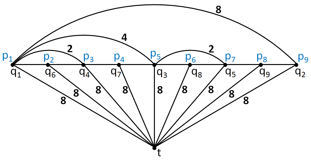
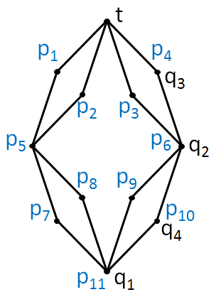
Uniform protocols. The designer chooses an order of the players without prior knowledge of the graph. The adversary constructs a worst-case graph, by simulating the adversary for the Greedy Algorithm of the OSTP [38], and places the players accordingly (see for example Figure 1(a),(b), the labels). Therefore the PoA of uniform ordered protocol is [22].
-
Universal protocols. The designer takes into account the graph; consider the worst-case graph for the Greedy Algorithm of the OSTP (illustrated in Figure 1(a),(b) for a small number of players). For the graph of Figure 1(a), choose the linear order dictated from the path (say from left to right). For the graph of Figure 1(b) order the vertices according to their distance from , . The adversary will choose and the positions of the players (). In both cases, it is not hard to see that, no matter which subset of players the adversary chooses, the PoA remains constant as grows.
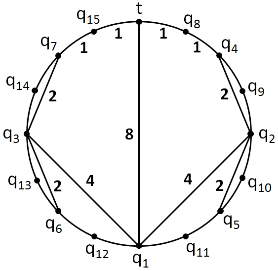
Example 2.
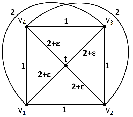
(Generalized weighted Shapley). In [22], it was shown that ordered protocols are essentially optimal among uniform protocols. In our model, the choice of the optimal method may depend on the underlying graph metric. Take the example in Figure 1(c). By using Shapley cost sharing the adversary can choose and in the Nash equilibrium , connect directly to and connects through . Regarding any ordered protocol, the square defined by the ’s contains a path of length where the middle vertex comes last in the order. The adversary will select this triplet of players, say . In the Nash equilibrium, connects directly to , and connect through . In both cases, the cost of the Nash equilibria is and the minimum Steiner tree that connects those vertices with has cost (by ignoring ) and therefore, PoA .
However the following (generalized Shapley) protocol, has . Partition the players into two sets . If players from both partitions appear on some edge, then the cost is charged only to players from . Players that belong to the same partition share the cost equally. One can verify that for all possible subsets of players this protocol produces only optimal equilibria.
Results.
We propose a framework for the design of (universal) network cost-sharing protocols with good equilibria, in situations where the designer has incomplete information about the input. We consider two different models, the adversarial and the stochastic. In both models, the designer has prior knowledge of the underlying metric but the requested subset of the players is not known and is activated either in an adversarial manner (adversarial model) or is drawn from a known probability distribution (stochastic model). The central question we address is: to what extent does prior knowledge of the metric help in good network design under uncertainty?
For the adversarial model, we first demonstrate that there exist classes of graph metrics where prior knowledge of the underlying metric can dramatically improve the performance of good network cost-sharing design. For outerplanar graph metrics, we provide a universal ordered cost-sharing protocol with constant PoA, against any choice of the adversary. This is in contrast to uniform protocols that ignore the graph and cannot achieve PoA better than in outerplanar metrics.
Our main technical result shows that there exist graph metrics, for which knowing the underlying metric does not help the designer, and any universal protocol has PoA of . This matches the upper bound of that can be achieved without prior knowledge of the metric [38, 22].
Then we switch to the stochastic model, where each player is independently activated according to some probability that is known to the designer. We show that there exists a randomized ordered protocol that achieves constant PoA. By using standard derandomization techniques [52, 48], we produce a deterministic ordered protocol that achieves constant PoA. We remark, that the first result holds also for the black-box model, where the probabilities are not known to the designer, but is allowed to draw independent (polynomially many) samples.
Our results for the adversarial model motivate the following question that is left open.
Open Question: For which metric spaces can one design universal protocols with constant PoA? What sort of structural graph properties are needed to obtain good guarantees?
Techniques.
We prove our main lower bound for the adversarial model in two parts. In the first part (Section 3) we bound the PoA achieved by any ordered protocol. Our origin is a well-known “zig-zag” ordered structure that has been used to show a lower bound on the Greedy Algorithm of the OSTP (see the labeled path in Figure 1(a)). The challenge is to show that high dimensional hypercubes exhibit such a distance preserving structure no matter how the vertices are ordered. Section 3 is devoted to this and we believe that this is of independent interest.
We show the existence proof by employing powerful tools from Extremal Combinatorics and in particular Ramsey Theory [35]. We are inspired by a Ramsey-type result due to Alon et al. [4], in which they show that for any given length , any -edge coloring of a high dimensional hypercube contains a monochromatic cycle of length . Unfortunately, we cannot immediately use their results, but we show a similar Ramsey-type result for a different, carefully constructed structure; we assert that every 2-edge coloring of high dimensional hypercubes contains a monochromatic copy of that structure. Then, we prescribe a special -edge-coloring that depends on the ordering of , so that the special subgraph preserves some nice labeling properties. A suitable subset of the subgraph’s vertices can be 1-embedded into a hypercube of lower dimension. Recursively, we show existence of the desired distance preserving structure.
In the second part (Section 4), we extend the lower bound to all universal cost-sharing protocols, by using the characterization of [22]. At a high level, we use as basis the construction for the ordered protocol and create “multiple copies”222Note that the standard complexity measure, to analyze the inefficiency of equilibria, is the number of participants, , and not the total number of vertices in the graph (see for example [5, 22]).. The adversary will choose different subsets of players, depending on whether the designer chose protocols “closer” to Shapley or to ordered. In the latter case, we use arguments from Matching Theory to guarantee existence of ordered-like players in one of the hypercubes.
For the stochastic model (Section 6), we construct an approximate minimum Steiner tree over a subset of vertices which are drawn from the known probability distribution. This tree is used as a base to construct a spanning tree, which determines a total order over the vertices. We finally produce a deterministic order by applying standard derandomization techniques [52, 48].
Related Work
Following the work of [5, 6], a long line of research studies network cost-sharing games, mainly focusing on the PoS of the Shapley cost-sharing mechanism. [5] showed a tight bound for directed networks, while for undirected networks several variants have been studied [14, 16, 21, 23, 28, 29, 45, 15] but the exact value of PoS still remains a big open problem. For multicast games, an improved upper bound of is known due to Li [45], while for broadcast games, a series of work [29, 44] lead finally to a constant due to Bilò et al. [16]. The PoA of some special equilibria has been also studied in [19, 20].
Chen, Roughgarden and Valiant [22] initiated the study of network cost-sharing design with respect to PoA and PoS. They characterized a class of protocols that satisfy certain desired properties (which was later extended by Gopalakrishnan, Marden and Wierman, in [33]), and they thoroughly studied PoA and PoS for several cases. Falkenhausen and Harks [51] studied parallel links and weighted players while Gkatzelis, Kollias and Roughgarden [31], focus on weighted congestion games with polynomial cost functions.
Close in spirit to universal cost-sharing protocols is the notion of Coordination Mechanisms [24] that provides a way to improve the PoA in cases of incomplete information. The designer has to decide in advance local scheduling policies or increases in edge latencies, without knowing the exact input, and has been used for scheduling problems [24, 39, 42, 8, 18, 26, 12, 1, 2] as well as for simple routing games [25, 13].
As discussed in Example 1, the analysis of the equilibria induced by ordered protocols corresponds to the analysis of Greedy Algorithm for the MST. In the uniform model, this corresponds to the analysis of the Greedy Algorithm [38, 7] for the (Generalized) OSTP [3, 9, 50], which was shown to be -competitive by Imase and Waxman [38] (-competitive for the Generalized OSTP by [7]). The universal model is closely related to universal network design problems [40], hence our choice for the term “universal”. In the universal TSP, given a metric space, the algorithm designer has to decide a master order so that tours that use this order have good approximation [46, 10, 37, 34, 40].
Much work has been done in stochastic models and we only mention the most related to our work. Karger and Minkoff [41] showed a constant approximation guarantee for the maybecast problem, where the designer needs to fix (before activation) some path for every vertex to the root. Garg et al. [30] gave bounds on the approximation of the stochastic online Steiner tree problem. A line of works [11, 34, 47, 48] has studied the a priori TSP. Shmoys and Talwar [48] assumed independent activations and demonstrated randomized and deterministic algorithms with constant approximations.
2 Model and definitions
Universal Cost-Sharing Protocols.
A multicast network cost-sharing game, is specified by a connected undirected graph , with a designated root and nonnegative weight for every edge , a set of players and a cost-sharing protocol. Each player is associated with a terminal333We abuse notation and use to refer both to the players and their associated vertices. , which she needs to connect with . We say that a vertex is activated if there exists some requested player associated with it. In the adversarial model the designer knows nothing about the set of activated vertices, while in the stochastic model, the vertices are activated according to some probability distribution which is known to the designer.
For any set of players, a cost-sharing method decides, for every subset , the cost-share for each player . A natural rule is that the shares for players not included in should always be , i.e. if , . W.l.o.g. each player is associated with a distinct vertex444 To see this, if there are two players with , for some , we modify the graph by connecting a new vertex with via a zero-cost edge and then we set and . Neither the optimum solution, nor any Nash equilibrium are affected by this modification.. For any graph and any set of players , a cost-sharing protocol assigns, for every , some cost-sharing method on .
Following previous work [22, 51], we focus on cost-sharing protocols that satisfy the following natural properties:
-
(1)
Budget-balance: For every network game induced by the cost sharing protocol , and every outcome of it, , for every edge with cost .
-
(2)
Separability: For every network game induced by the cost sharing protocol , the cost shares of each edge are completely determined by the set of players using it.
-
(3)
Stability: In every network game induced by the cost-sharing protocol , there exists at least one pure Nash equilibrium, regardless of the graph structure.
We call a cost-sharing protocol universal, if it satisfies the above properties for any graph , and it assigns the cost-sharing method to edge based only on knowledge of (without knowledge of 555The methods should be defined on , since every vertex is potentially associated with some player.) for the adversarial model, while in the stochastic the method can in addition depend on . Due to the characterization in [22], we restrict ourselves to the family of generalized weighted Shapley protocols666[22] characterizes the linear protocols (for every edge of cost , it assigns the method , where is the method it assigns to any edge of unit cost) to be the generalized weighted Shapley protocols. They further showed that for any non-linear protocol, there exists a linear one with at most the same PoA..
Generalized Weighted Shapley Protocol (GWSP).
The generalized weighted Shapley protocol (GWSP) is defined by the players’ weights (parameters) and an ordered partition of the players . An interpretation of is that for , players from “arrives” before players from . More formally, for every edge of cost , every set of players that uses and for , the GWSP assigns the following method to :
In the special case that each contains exactly one player, the protocol is called ordered. The order of the sets indicates a permutation of the players, denoted by .
(Pure) Nash Equilibrium (NE).
We denote by the strategy space of player , i.e. the set of all the paths connecting to . denotes an outcome or a strategy profile, where for all . As usual, denotes the strategies of all players but . Let be the set of players using edge under . The cost share of player induced by ’s is equal to . The players’ objective is to minimize their cost share . A strategy profile is a Nash equilibrium (NE) if for every player and every strategy ,
Price of Anarchy (PoA).
The cost of an outcome is defined as , while is the optimum solution. The Price of Anarchy (PoA) is defined as the worst-case ratio of the cost in a NE over the optimal cost in the game induced by . In the adversarial model the worst-case is chosen, while in the stochastic model is drawn from a known distribution . Formally, in the adversarial model we define the PoA of a protocol on as
where is the set of all NE of the game induced by and on .
In the stochastic model, the PoA of , given and is
In both models the objective of the designer is to come up with protocols that minimize the above ratios. Finally, the Price of Anarchy for a class of graph metrics , is defined as
Graph Theory.
For every graph , we denote by and the set of vertices and edges of , respectively. For any , denotes an edge between and and denotes the shortest distance between and in ; if is clear from the context, we simply write . A graph is an induced subgraph of , if is a subgraph of and for every , if and only if . is a distance preserving (isometric) subgraph of , if is a subgraph of and for every , .
3 Lower Bound of Ordered Protocols
The main result of this section is that the PoA of any ordered protocol is which is tight. We formally define (Definition 4) the ‘zig-zag’ pattern of the lower bounds of the Greedy Algorithm of the OSTP (see Example 1(a) and Figure 2). Then the main technical challenge is to show that for any ordering of the vertices of high dimensional hypercubes, there always exists a distance preserving path, such that the order of its vertices follows that zig-zag pattern. Finally, by connecting any two vertices of the hypercube with a direct edge of suitable cost, similar to the example in Figure1(a), we get the final lower bound construction.
Definition 3 (Classes).
For , and for a path graph of vertices, we define a partition of the vertices into classes, , as follows: Class contains the endpoints of , . For every , . For , and , we say that belongs to a lower class than (and belongs to a higher class than ).
As an example, consider the path , where . Then, , , and . Note that always and for , .
For and , we define the parents of as , i.e. the closest vertices that belong to lower classes. Remark that for all i) the cardinality of is , ii) the vertices of belong to lower classes than , iii) all vertices between and any vertex of belong to higher classes than . We are now ready to define the “zig-zag” pattern.
Definition 4 (Zig-zag pattern).
We call a path graph , with distinct integer labels , zig-zag, and we denote it by , if for every , for all .
An example of such a path for is shown in Figure 2. Our main result of this section is that there exist graphs, high dimensional hypercubes, such that for any order , always appears as a distance preserving subgraph. Our proof is existential and uses Ramsey theory.
Proof Overview: The proof is by induction and in the inductive step our starting point is the -th dimensional hypercube . Given an ordering/labeling of the vertices of we first show that contains a subgraph which is isomorphic to a ‘pseudo-hypercube’ () where the labeling of its vertices satisfies a special property (to be described shortly). is defined by replacing each edge of by a 2-edge path (of length two)777See of Definition 7 and Figure 3a for an illustration.
Labeling property: For the subgraph we require that all such newly formed 2-edge paths, are paths, i.e. the label of the middle vertex is greater than the labels of the endpoints (Figure 3(a) shows such a labeling).
Next, we contract all such 2-edge paths of into single edges, resulting in a graph isomorphic to ; this is the hypercube used for the next step. Note that each contracted edge still corresponds to a path in . Therefore, after recursive steps, each edge corresponds to a path of . Further, note that such a path is a path, due to the labeling property that we preserve at each step. We require that, at the end of the last inductive step, (a single edge), and (by unfolding it) we show that this edge corresponds to a distance preserving subgraph of the original graph/hupercube. At each step, ; the relation between and is determined by a Ramsey-type argument. We next describe the basic ingredients that we use to show existence of . We apply a coloring scheme to the edges of that depends on the order of the vertices.
Coloring Scheme: Consider as a bipartite . For any edge , with and , if the ’s label is smaller than ’s, we paint the edge blue, otherwise we paint it red.
By a Ramsey-type argument we show that has a monochromatic subgraph isomorphic to a specially defined graph ; is carefully specified in such a way that it contains at least two subgraphs isomorphic to pseudo-hypercubes . The special property of those two subgraphs is described next.
Let and be the two half cubes888The two half-cubes of order are formed from by connecting all pairs of vertices with distance exactly two and dropping all other edges. of and let and . Observe that if is a subgraph of then the corresponding is an induced subgraph of either or . We carefully construct such that it contains subgraphs and isomorphic to , whose corresponding ’s are induced subgraphs of and , respectively. The color of determines which of the and will serve as the desired . In particular, if the color is blue, then for every edge , with and , it should hold that ’s label is smaller than ’s and therefore the labeling property is satisfied for ; similarly, if the color is red, serves as .
Proof Roadmap. The whole proof of the lower bound proceeds in several steps in the following sections. In Section 3.1 we give the formal definition of the subgraph of a hypercube . Section 3.2 is devoted to show that every -edge coloring of a (suitably) high dimensional hypercube contains a monochromatic copy of (Lemma 6), by using Ramsey theory. Then, in Section 3.3 we show that, for any ordering of the vertices of , we can define a special -edge-coloring , so that there exists a subgraph of that preserves the Labeling property (Lemma 8). At last, in Section 3.4, by a recursive application of the combination of the Ramsey-type result and the coloring, we prove the existence of the zig-zag path in high dimensional hypercubes (Theorem 9). We then show how to construct a graph that serves as lower bound for all ordered protocols (Theorem 11). This is done by connecting any two edges of the hypercube with a direct edge of appropriate cost, similar to the example in Figure 1(a).
Definitions and notation on Hypercubes.
We denote by (for ) the set of integers , but when , we simply write . We follow definitions and notation of [4]. Let be the graph of the -dimensional hypercube whose vertex set is . We represent a vertex of by an -bit string , where . By or we denote the concatenation of an -bit string with an -bit string , i.e. . is the concatenation of its bits. An edge is defined between any two vertices that differ only in a single bit. We call this bit, flip-bit, and we denote it by ‘’. For example, are two vertices of and is the edge that connects them. The distance between two vertices is defined by their Hamming distance, . For a fixed subset of coordinates , we extend the definition of the distance as follows,
We define the level of a vertex by the number of ‘ones’ it contains, . We denote by the set of vertices of level . We define the prefix sum of an edge , where the flip-bit is in the -th coordinate, by . We represent any ordering of , by labeling the vertices with labels , where label corresponds to ranking in .
3.1 Description of
For a positive integer , we define a graph that is a restriction of on . A vertex of is defined by concatenations of pairs and and a single pair that appears in the second half of the string. A vertex of is defined by concatenations of and . A vertex of is defined by concatenations of and , one pair that appears on the first half of the string, and one pair that appears on the second half. For example, for , , , . More formally, let , then the subsets are defined as follows:
Observe that is bipartite with vertex partitions and , as vertices of belong to level , while vertices of to level .
Lemma 5.
Every pair of vertices with , have a unique common neighbor . Also, every pair of vertices , with , have a unique common neighbor .
Proof.
Recall that (by definition) if then should coincide in all but the coordinates. For the first statement, observe that the premises of the Lemma hold only if there exists such that and (or the other way around), in which case the required vertex from has ; the rest of the bits are the same among . For the second statement, the premises of the Lemma hold only if there exists an such that and (or the other way around), in which case the required vertex from has and the rest of the bits are the same among . ∎
3.2 Ramsey-type Theorem
Lemma 6.
For any positive integer , and for sufficiently large , any 2-edge coloring of , contains a monochromatic copy of 999The result could be extended to any (fixed) number of colors, but we need only two for our application..
Proof.
The proof follows ideas of Alon et al. [4]. Consider a hypercube , with sufficiently large to be determined later, and some arbitrary -edge-coloring . Let be the set of edges between vertices of and (recall that ).
Each edge contains 1’s, a flip-bit represented by and the rest of the coordinates are . Moreover, is uniquely determined by its non-zero coordinates and its prefix sum (number of s before the flip-bit). Therefore, the color defines a coloring of the pair , i.e. . For each subset of coordinates, we denote by the color induced by the edge coloring. The coloring of all subsets defines a coloring of the complete -uniform hypergraph of using colors.
By Ramsey’s Theorem for hypergraphs [35], there exists such that for any there exists some subset of size such that all -subsets have the same color . Therefore, for every and , it is . Since takes values and there are only two different colors, there must exist indices with the same color , for all , and .
It remains to show that the graph formed with the edges that are determined by those prefix sums, contains a monochromatic copy of . We will show this by constructing those edges from (the set of edges of ). By inserting blocks of ’s of suitable length among the bits of the edges of , we construct the bits at the coordinates of . The rest of the bits () are set to zero.
Let be a string of 1’s and define for , and . For any edge , we insert at the beginning of the string, for we insert between and and for we insert the string after . Recall that each edge of contains exactly zero bits. Also notice that Therefore, in total we have bits (same as the size of ) and non-zero bits (same as the size of ). These bits are put precisely at the coordinates of . The rest of the coordinates are filled with zeros.
It remains to show that for such edges the prefix of the flip-bit is always one of the . This would imply that all these edges are monochromatic. Furthermore, all but coordinates are fixed and the coordinates form exactly the sets ; therefore, the monochromatic subgraph is isomorphic to .
For any edge , let the flip-bit be at position:
-
•
for . Its prefix is , where the term corresponds to the number of pairs with , each of which contributes to the prefix with a single .
-
•
for . Since , . Then the prefix equals to .
-
•
or for . For such , and all other pairs belong to . Therefore, the prefix is equal to .
∎
3.3 Coloring based on the labels
This part of the proof shows that for any ordering of the vertices of a hypercube , there is a -edge coloring with the following property: in the monochromatic , either all the vertices of or all the vertices of have neighbors in with only higher label. This implies a desired labeling property for a subgraph of , the structure of which is defined next.
Definition 7.
We define to be a subdivision of , by replacing each edge by a path of length . is simply . We denote by the set of all pairs of vertices , which correspond to edges of ; is the corresponding path in . For every , we denote by the middle vertex of .
| (a) | (b) |
In the next lemma we show that for any ordering of the vertices of , there exists a subgraph isomorphic to , such that the ‘middle’ vertices have higher label than their neighbors (Labeling Property).
Lemma 8.
For any positive integer , for all and for any ordering of , there exists a subgraph of that is isomorphic to , such that for every , it is .
Proof.
Choose a sufficiently large as in Lemma 6. Partition the vertices of into sets of vertices of odd and even level, respectively. We color the edges of as follows. For every edge with and , if , then paint blue. Otherwise paint it red. Therefore, for every blue edge, the endpoint in has smaller label than the endpoint in . The opposite holds for any red edge.
Lemma 6 implies that contains a monochromatic copy (blue or red) of . Recall that is bipartite between vertices of levels and and that and . Let be the subset of the coordinates that correspond to vertices of . Also let and be the subsets of the first and the last coordinates of , respectively.
First suppose that is blue. An immediate implication of our coloring is that for every edge with , it must be . Fix a -bit string that corresponds to a permissible bit assignment to the coordinates of some vertex in (see Section 3.1). Define as the subset of vertices of where the coordinates are set to . Recall that each of the first pairs , , of a vertex , may take any of the two bit assignments and . Hence, .
Observe that we can embed into with distortion 1 and scaling factor , by mapping the first pairs of bits into single bits; map to and to . Every two vertices with distance in , have distance in . For every with , Lemma 5 implies that there exists , such that . Therefore, . Take the union of all such vertices , then induces a subgraph isomorphic to , that fulfills the labeling requirements.
The case of being red is similar. We focus only on vertices . Fix now a -bit string that corresponds to a permissible bit assignment of the coordinates of a vertex in . Define as the subset of vertices of where the coordinates are set to . Similarly, we can embed into with distortion 1 and scaling factor .
For every with , where the coordinates are fixed to , Lemma 5 implies that there exists , such that . Therefore, . Take the union of all such vertices , then induces a subgraph isomorphic to , that fulfills the labeling requirements. ∎
3.4 Lower Bound Construction
Now we are ready to prove the main theorem of this section.
Theorem 9.
For every positive integer , and for sufficiently large , there exists a graph such that, for every ordering of its vertices, it contains a zig-zag distance preserving path .
Proof.
Let be a function as in Lemma 6. We recursively define the sequence , such that and , for . We will show that is the graph we are looking for.
Claim 10.
For every , and for any vertex ordering of , it contains a subgraph isomorphic to , such that for every , is a distance preserving path isomorphic to .
Proof.
The proof is by induction on . As a base case, is the graph itself. An edge is trivially a path , for any . Suppose now that contains a subgraph isomorphic to , for some , such that for every , is a path . It is sufficient to show that contains a subgraph isomorphic to , such that for every , is a path .
For every , if we replace with a direct edge , the resulting graph is a copy of . Applying Lemma 8 on , guarantees the existence of a subgraph isomorphic to (), where for every , . Each of the edges and of are replaced by a path in . Therefore, is a copy of , with being a path . ∎
We now argue that the resulting is a distance preserving path. Our analysis indicate a sequence of hypercubes . Recall that in Lemma 8, in order to get from we mapped to and to and the vertices of did not differ in any other bit but the ones we mapped. Consider now the two vertices of with bit-strings and , respectively. Their Hamming distance in their original bit representation (in ) should be , the same with their distance in . Moreover, if any two vertices of are closer in than in , then this would contradict the fact that . ∎
Finally we extend so that for any order of its vertices, a path exists along with the shortcuts as shown in the example in Figure 1(a).
Theorem 11.
Any ordered universal cost-sharing protocol on undirected graphs admits a PoA of , where is the number of activated vertices.
Proof.
Let for some positive integer . From Theorem 9, we know that for any vertex ordering of there is a distance preserving path .
We use as a basis to construct the weighted graph with vertex set , where is the designated root. We connect every pair of vertices with a direct edge of cost , if is one of its endpoints, otherwise its cost is (similar to Figure 1(a)).
The adversary selects to activate the vertices of , and the lower bound follows; in the NE the players choose their direct edges to connect with one of their parents (see at the beginning of Section 3 for the term “parent”). ∎
4 Lower Bound for all universal protocols
In this section, we exhibit metric spaces for which no universal cost-sharing protocol admits a PoA better than . Due to the characterization of [22], we can restrict ourselves in generalized weighted Shapley protocols (GWSPs). We follow the notation of [22], and for the sake of self-containment we include here the most related definitions and lemmas.
4.1 Cost-Sharing Preliminaries
A strictly positive function is an edge potential on , if it is strictly increasing, i.e. for every , , and for every , For simplicity, instead of , we write . A cost-sharing protocol is called potential-based, if it is defined by assigning to each edge of cost , the cost-sharing method , where for every and ,
Let and be two cost-sharing protocols for disjoint sets of vertices and , with methods and , respectively. The concatenation of and is the cost sharing protocol of the set , with method defined as
Note that the concatenation of two protocols for disjoint sets of vertices defines an order among these two sets. The GWSPs are concatenations of potential-based protocols.
Lemma 12.
(Lemma of [22]). Let be an edge potential on and the induced (by ) cost-sharing method, for unit costs. For and a constant , with , let be a subset of vertices with , for every . If , then for any ,
Lemma 13.
(Lemma of [22]). Let be an edge potential on , and be the cost-sharing method induced by , for unit cost. For any two vertices , such that : and for every ,
4.2 Lower Bound
The following two technical lemmas will be used in our main theorem.
Lemma 14.
Let be a finite set of size , and be a partition of , with , for all . Then, for any coloring of such that no more than elements have the same color, there exists a rainbow subset (i.e. for all ), with for every .
Proof.
Given the partition of and the coloring , we construct a bipartite graph , where is the set of colors used in . For every we create a set of size ; then . If color is used in , we add an edge for all .
Each color appears in at most distinct sets, and since for each there are vertices (), the degree of is at most . On the other hand, each has size and hence, it has at least different colors. Therefore, the degree of each vertex of is at least .
Consider any set , and let be the set of edges with at least one endpoint in . If denotes the set of neighbors of , observe that . By using the degree bound on vertices of , and by using the degree bound on vertices of , . Therefore, . By Hall’s Theorem there exists a matching which covers every vertex in . Each vertex in is matched with a distinct color and therefore in each there exists a subset with at least elements with distinct colors; let be such a subset with exactly elements. In addition the colors in different subsets should be distinct by the matching. Then, . ∎
Lemma 15.
Let be a partition of , with , for all . Then, there exists a subset with exactly one element from each subset , such no two distinct are consecutive, i.e. for every , .
Proof.
For every , let . W.l.o.g we can assume that the ’s are in increasing order with respect to and in addition that ’s are sorted such that , for all (otherwise rename the elements recursively to fulfill the requirement). Then, it is not hard to see that can serve as the required set. ∎
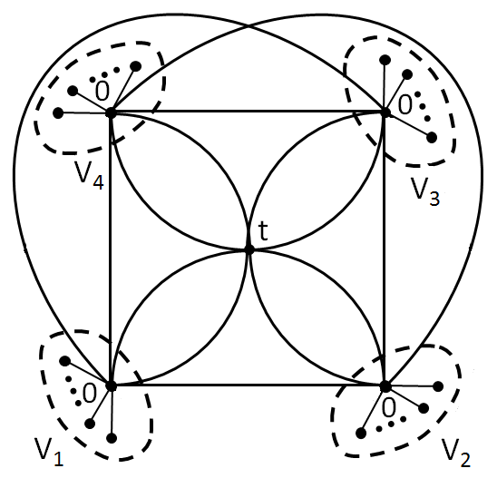
Now we proceed with the main theorem of this section. We create a graph where every GWSP has high PoA. At a high level, we construct a high dimensional hypercube with sufficiently large number of potential players at each vertex (by adding many copies of each vertex connected via zero-cost edges). Moreover, we add shortcuts among the vertices of suitable costs and we connect each vertex with via two parallel links with costs that differ by a large factor (see Figure 4). If the protocol induces a large enough set of potential players with Shapley-like values in some vertex, then it is a NE that all these players follow the most costly link to . Otherwise, by using Lemmas 14 and 15 we show that there exists a set of potential players , with ordered-like values, one at each vertex of the hypercube. Then, by using the results of Section 3, there exists a path where the vertices are zig-zag-ordered.
The separation into these two extreme cases was first used in [22]. The crucial difference, is that for their problem the protocol is specified independently of the underlying graph, and therefore the adversary knows the case distinction (ordered or shapley) and bases the lower bound construction on that. However, our problem requires more work as the graph should be constructed in advance, and should work for both cases.
Theorem 16.
There exist graph metrics, such that the PoA of any universal cost-sharing protocol is at least , where is the number of activated vertices.
Proof.
Let be the number of activated vertices with , (hence ).
Graph Construction. We use as a base of our lower bound construction, a hypercube , with edge costs equal to and as in Theorem 9. Based on , for we construct the following network with vertices, plus the designated root . We add to direct edges/shortcuts as follows: for every two vertices of distance , for , we add an edge/shortcut, , with cost equal to . Moreover, for every vertex of , we create new vertices, each of which we connect with via a zero-cost edge. Let be the set of these vertices (including ). Finally, we add a root , which we connect with every vertex of , via two edges and , with costs and , respectively. We denote this new network by (see Figure 4).
We will show that any GWSP for has PoA . Any GWSP can be described by concatenations of potential-based cost-sharing protocols for a partition of the into subsets , where is induced by some edge potential . Following the analysis of Chen, Roughgarden and Valiant [22], we scale the ’s such that for every , . For nonnegative integers and for , we form subgroups of vertices , for each , as (note that some of ’s may be empty).
The adversary proceeds in two cases, depending on the intersection of the ’s with the ’s.
Shapley-like cost-sharing. Suppose first that there exist and such that , and take a subset with exactly vertices. The adversary will request precisely the set . Budget-balance implies that there exists some vertex which is charged at most proportion of the cost. Moreover, Lemma 12 implies that, all are charged at most proportion of the cost.
Note that there is a NE where all players follow the edge , with cost ; no player’s share is more than and any alternative path would cost at least . However, the optimum solution is to use the parallel link of cost . Therefore, the PoA is for this case.
Ordered-like cost-sharing. If there is no such with at least vertices, then for all and , which means that each has size of at most . For every , we group consecutive sets (starting from ) into sets , such that each , (except perhaps from the last one), contains exactly nonempty ’s. The last contains at most nonempty sets. Consider the lexicographic order among ’s, i.e. if either or and . Rename these sets based on their total order as ’s. The size of each is at most .
Now we apply Lemma 14 on the set , for and , by considering the subsets as the partition of (recall that ). As a coloring scheme, we color all the vertices of each with the same color and use different colors among the sets . Lemma 14 guarantees that for each there exists of size , such that every belongs to a distinct .
The order of ’s suggests an order of the vertices of . Since the ’s form a partition of , Lemma 15 guarantees the existence of a subset , such that contains exactly one vertex from each and there are no consecutive vertices in . This means that contains exactly one vertex from each set and all these vertices belong to different and non-consecutive sets .
To summarize, so far we know that:
-
(i)
for any pair of vertices , either and come from different ’s or their and values differ by a factor of at least (since there exist at least nonempty sets between the ones that and belong to).
-
(ii)
is a copy of (by ignoring zero-cost edges).
Let be the order of vertices of (recall that they are ordered according to the ’s they belong to). Theorem 9 guarantees that there always exists at least one distance preserving path (see Definition 4). Let be the vertices of excluding the last class (see Definition 3). The adversary will activate this set (). It remains to show that there exists a NE, the cost of which is a factor of away from optimum. We will refer to these vertices as , based on their order , from smaller label to larger, and let player be associated with .
Let be the class of strategy profiles which are defined as follows:
-
•
and , where is the shortcut edge between and .
-
•
From to , let be one of ’s parents in the class hierarchy (we refer the reader to the beginning of Section 3); then , where is the shortcut edge between and .
We show in Claim 17 that there exists a strategy profile which is a NE. has cost:
However, there exists the solution , which has cost of . Therefore, the PoA is .
Claim 17.
There exists which is a Nash equilibrium.
Proof.
We prove the claim by using better-response dynamics. Note that any GWSP induces a potential game for which better-response dynamics always converge to a NE (see [22, 33]). We start with some and we prove that, after a sequence of players’ best-responses, we end up in . Proceeding in a similar way we eventually converge to , which is the required NE.
We next argue that for any , players and , have no incentive to deviate from (argument (a)) and (arguments (b)), respectively. We further show that, given any strategy profile , there exists some such that: for every player , if are the strategies of the other players, prefers to (arguments (c)-(e)). We define the desired recursively as follows: , and from to , . If then we set , otherwise we choose a path from arbitrarily.
We first give some bounds on players’ shares.
-
1.
Let be any set of players that use some edge of cost and let be the one with the smallest label. The total share of players is upper bounded by (Lemma 13). Moreover, ’s share is at least .
-
2.
The total cost of any under , is at most . This is true because, for every player with , the first edge of is a shortcut to reach one of ’s parents, with cost at most , where is the class that belongs to. Therefore, the cost of is at most .
-
3.
By combining the above two arguments, under , the total share of player for the edges of at which she is not the first according to , is at most .
Here, we give the arguments for players and .
-
(a)
The share of player under is at most and any other path would incur a cost strictly greater than .
-
(b)
The share of player under is at most (argument ), whereas if she doesn’t connect through , her share would be at least . Moreover, if she connects to through but by using any other path rather than the shortcut , the total cost of that path is at least . Player is first according to at that path and by argument , her share is at least .
We next give the required arguments in order to show that is a best response for player under . In the following, let and let be the parent of such that . Also let be the predecessor of , according to , that is first met by following from to .
-
(c)
Suppose that .
-
•
Assume that doesn’t use the shortcut . The subpath of from to contains edges at which is first according to of total cost at least . By argument , her share is at least .
-
•
Assume that doesn’t use . The subpath of from to contains edges at which is first according to of total cost at least (the minimum distance between two activated vertices). By argument , her share is at least , where is at most her share for (argument ).
-
•
-
(d)
Suppose that is ’s other parent. If , the above arguments still hold and so . Otherwise, by the definition of , either , or .
-
(e)
Suppose that is not a parent of . Player ’s share in is at most for her first edge/shortcut and at most for the rest of her path (argument ). However, all edges that are used by players that precedes in have cost at least . Therefore, in , player is the first according to for edges of total cost at least . This implies a cost-share of at least (argument ). But for and , .
We now describe a sequence of best-responses from some to ( is constructed based on as described above). We follow the order of the players and for each player we apply her best response. First note that players and have no better response, so and . When we process any other player , we have already processed all her predecessors in and so, the strategies of the other players are . Therefore, is the best response for (it may be that , where no better response exists for ). The order that we process the vertices guarantees that .
∎
∎
5 Outerplanar Graphs
In this section we show that there exists a class of graph metrics, prior knowledge of which can dramatically improve the performance of good network cost-sharing design. For outerplanar graphs, we provide a universal cost-sharing protocol with constant PoA. In contrast, we stress that uniform protocols cannot achieve PoA better than , because the lower bound for the greedy algorithm of the OSTP can be embedded in an outerplanar graph (see Figure 5(a) for an illustration).
We next define an ordered universal cost-sharing protocol , and we show that it has constant PoA. W.l.o.g. we assume that the metric space is defined by a given biconnected outerplanar graph101010If it is not already biconnected, we turn it into an equivalent biconnected graph, by appropriately adding edges of infinity cost. By equivalent we mean that any NE outcome and the minimum Steiner tree solution remain unchanged after the transformation. Equivalence is obvious since we only add edges of infinity costs that cannot be used in neither any NE nor the minimum Steiner tree outcome.. Every biconnected graph admits a unique Hamiltonian cycle [49] that can be found in linear time [27]. orders the vertices according to the cyclic order in which they appear in the Hamiltonian tour, starting from and proceeding in a clockwise order . In Figure 5(a), .
 |

|
As a warm-up, we first bound from above the PoA of for cycle graphs, and then extend it to all outerplanar graphs.
Lemma 18.
The PoA of in cycle graphs is at most .
Proof.
Consider a cycle graph and let be the set of the activated vertices. Let be the minimum Steiner tree (path) that connects , and , be its two endpoints. Note that minimality of implies that . and partition into two paths and divides further into two paths , . Let and be the activated vertices of and , respectively. W.l.o.g., assume that and , for all .
Consider any NE, . We bound from above the share of each player , by its distance from their immediate predecessor in , as follows. By adopting the convention that ,
Also . Overall,
∎
Theorem 19.
The PoA of in outerplanar graphs is at most .
Proof.
Based on the previous discussion, it is sufficient to consider only biconnected outerplanar graphs with non-negative costs, including infinity. Let be any such graph with being the set of activated vertices.
Let be the minimum Steiner tree that connects , and be the unique Hamiltonian tour of , forming its outer face. Let be the set of non-crossing chords of that belong to . Then forms cycles , where every pair , are either edge-disjoint or they have a single common edge belonging to . On the other hand, each edge of belongs to exactly one and each edge of belongs to exactly two ’s. Figure 5(b) provides an illustration.
For every , let be the activated vertices that lie in and be the vertex that is first in among . W.l.o.g. assume that, for all , (then ). Also let be the subgraph of that intersects with . Then should be a path connecting .
Consider any NE, . We show separately that the shares of all are bounded by and the shares of all ’s are bounded by .
For the first case we use Lemma 18. For any cycle , by considering as the root, Lemma 18 provides a bound on the shares of . So, . Recall, that each edge of belongs to at most two ’s, so by summing over all ,
The second case requires more careful treatment. The endpoints of the edges of divide into a partition of nonzero-length arcs, , named based on their clockwise appearance in , starting from an arc containing . For every , let and be the two endpoints of . The share of each can be bounded by its distance from , for (recall that ). Let be an arc that lies, then
We next upper bound by . Note that each arc belongs to exactly one and every contains at least one such arc (otherwise would have a cycle). We concentrate to a specific and show that the portion of associated with ’s arcs is upper bounded by .
Let be the arcs belonging to and , be the endpoints of . Also let be an arc containing . Recall that is a path and every edge of belongs to . Therefore, contains entirely all but one , say (see also Figure 5(b)). We examine the two cases of and separately.
Case 1: , (as endpoints of edges of ) and are vertices of the path . Therefore, either some path from to or some path from to belongs to ; w.l.o.g. assume that it is some path from to . Then . Moreover, since and are vertices of , .
Case 2: Similarly, . Also and are vertices of and hence, .
To sum up, in both cases it holds that
By summing over all , Finally, by summing over the whole , . ∎
6 Stochastic Network Design
In this section we study the stochastic model, where the set of active vertices is drawn from some probability distribution . Each vertex is activated independently with probability ; the set of the activated vertices are no longer picked adversarially, but it is sampled based on the probabilities ’s, i.e., the probability that set is active is . On the other hand, the probabilities ’s (and therefore ), are chosen adversarially. The cost sharing protocol is decided by the designer without the knowledge of the activated set and the designer may have knowledge of or access to some oracle of .
We show that there exists a randomized ordered protocol that achieves constant PoA. This result holds even for the black-box model [48], meaning that the probabilities are not known to the designer, however she is allowed to draw independent (polynomially many) samples. On the other hand, if we assume that the probabilities ’s are known to the designer, there exists a deterministic ordered protocol that achieves constant PoA. We note that both protocols can be determined in polynomial time.
The result for the randomized protocol depends on approximation ratios of the minimum Steiner tree problem. More precisely, given an -approximate minimum Steiner tree, we show an upper bound of . The approximate tree is used in our algorithm as a base in order to construct a spanning tree, which finally determines an order of all vertices; the detailed algorithm is given in Algorithm 1. This algorithm and its slight variants have been used in different contexts: rend-or-buy problem [36], a priori TSP [48] and, stochastic Steiner tree problem [30].
-
•
Choose a random set of vertices by drawing from distribution and construct an -approximate minimum Steiner tree, , over .
-
•
Connect all other vertices with their nearest neighbor in (by breaking ties arbitrarily).
-
•
Double the edges of that tree and traverse some Eulerian tour starting from . Order the vertices based on their first appearance in the tour.
Theorem 20.
Given an -approximate solution of the minimum Steiner tree problem, has PoA at most .
Proof.
Let be the order of all vertices , defined by , and be the random set of activated vertices that require connectivity with . For the rest of the proof we denote by a minimum spanning tree over .
Let be the vertices of as appeared in and the strategy profile be a NE of set . Under the convention that , for all . We construct a tree from the of Algorithm 1, by connecting only all vertices of with their nearest neighbor in (by breaking ties in accordance to Algorithm 1). Note that, by doubling the edges of , there exists an Eulerian tour starting from , where the order of the vertices (based on their first appearance in the tour) is restricted to the set . Therefore, . By combining the above,
| (1) |
Let be the distance of from its nearest neighbor in . In the special case that , we define Then,
| (2) |
We use an indicator which is when and otherwise; then . By taking the expectation over and ,
Since and are independent samples we can bound the second term as:
| (3) | |||||
The last equality holds since is the distance of from its nearest neighbor in and it is independent of the event . For the inequality, is upper bounded by the minimum distance of from its parent in the . Let be the minimum Steiner tree over , then it is well known that . Overall,
∎
By applying the -approximation algorithm of [17] we get the following.
Corollary 21.
has PoA at most .
Theorem 22.
There exists a deterministic ordered protocol with PoA at most .
Proof.
We use derandomization techniques similar to [52, 48] and for completeness we give the full proof here. First we discuss how we can get a PoA of , if we drop the requirement of determining the protocol in polynomial time. Similar to the proof of Theorem 20 we define the tree for the random activated set as follows: we construct from the of Algorithm 1, by connecting only all vertices of with their nearest neighbor in (by breaking ties in accordance to Algorithm 1). We apply the standard derandomization approach of conditional expectation method on . More precisely, we construct a deterministic set to replace the random in Algorithm 1, by deciding for each vertex of , one by one, whether it belongs to or not. Assume that we have already processed the set and we have decided that for its partition , and (starting from and ). Let be the next vertex to be processed. From the conditional expectations and the independent activations we know that
meaning that
| either | ||||
| or |
In the first case we add in and in the second case we add in . Therefore, after processing all vertices, . If we replace the sampled of Algorithm 1 with the deterministic set , we can get the same bound on the PoA with the randomized protocol of Theorem 20.
However, the value of seems difficult to be computed in polynomial time; the reason is that it involves the computation of which seems hard to be handled. To overcome this problem we use an estimator of , which is constant away from the optimum , where is the minimum Steiner tree over . Following [52, 48], we use the optimum solution of the relaxed Connected Facility Location Problem (CFLP) on in order to construct a feasible solution of the relaxed Steiner Tree Problem (STP) for a given set . We show that the objective’s value of the fractional STP for is constant away from and that its (conditional) expectation over can be efficiently computed. This quantity is used in order to construct the estimator . We apply the method of conditional expectations on and after processing all vertices, by using the primal-dual algorithm [32], we compute a Steiner tree on with cost no more than twice the cost of the fractional solution.
In the rooted CFLP, a rooted graph is given and the designer should select some facilities to open, including , and connects them via some Steiner tree . Every other vertex is assigned to some facility. The cost of the solution is ( times the cost of , plus the distance of every other vertex from its assigned facility. Our analysis requires to consider a slightly different cost of the solution, which is the cost of , plus the distance of every other vertex from its assigned facility multiplied by . In the following LP relaxation of the CFLP, and are - variables indicate, respectively, if and whether the vertex is assigned to facility . denotes the set of edges with one endpoint in and the other in , denotes the minimum distance between vertices and in and is the cost of edge .
| LP1: CFLP | |||
|---|---|---|---|
| subject to | = | 1 | |
| and | |||
Let be the optimum solution of LP1.
Claim 23.
.
Proof.
Given a set , for every edge ( is the minimum Steiner tree over ) let and for let . For every let if is ’s nearest neighbor in . Set the rest of equal to . Note that this is a feasible solution of LP1 with objective value . By taking the expectation over ,
∎
By using the solution , we construct a feasible solution for the following LP relaxation of the STP over some set .
| LP2: STP over | |||
|---|---|---|---|
| subject to | |||
We define if lies in the shortest path between and and it is otherwise. For every edge we set .
Claim 24.
is a feasible solution for LP2.
Proof.
The proof is identical with the one in [52] but we give it here for completeness. Consider any set such that and let . It follows that
For the last inequality, note that should be for at least one since and . ∎
Claim 25.
Let be the cost of the objective of LP2 induced by the solution . Then .
Proof.
∎
Observe that due to the expression of we can efficiently compute any conditional expectation ; this is because
We further define . We can also efficiently compute any conditional expectation (Claim 2.1 of [52]). We are ready to define our estimator:
Our goal is to define a deterministic set to replace the sampled of Algorithm 1. We process the vertices one by one and we decide if they belong to by using the model conditional expectations on . More specifically, assume that we have already processed the sets and (starting from and ) such that and . Let be the next vertex to be processed. From the conditional expectations and the independent activations we know that If we add to , otherwise we add to . After processing all vertices and by using Claims 23 and 25,
Let be the Steiner tree over computed by the primal-dual algorithm [32]. Then,
By combining inequalities (1) and (2) (after replacing by and by ) with all the above, we have that
∎
References
- [1] Fidaa Abed, José R. Correa, and Chien-Chung Huang. Optimal coordination mechanisms for multi-job scheduling games. In Algorithms - ESA 2014 - 22th Annual European Symposium, Wroclaw, Poland, September 8-10, 2014. Proceedings, pages 13–24, 2014.
- [2] Fidaa Abed and Chien-Chung Huang. Preemptive coordination mechanisms for unrelated machines. In Algorithms - ESA 2012 - 20th Annual European Symposium, Ljubljana, Slovenia, September 10-12, 2012. Proceedings, pages 12–23, 2012.
- [3] Noga Alon and Yossi Azar. On-line Steiner trees in the euclidean plane. Discrete & Computational Geometry, 10:113–121, 1993.
- [4] Noga Alon, Rados Radoicic, Benny Sudakov, and Jan Vondrák. A ramsey-type result for the hypercube. Journal of Graph Theory, 53(3):196–208, 2006.
- [5] Elliot Anshelevich, Anirban Dasgupta, Jon M. Kleinberg, Éva Tardos, Tom Wexler, and Tim Roughgarden. The price of stability for network design with fair cost allocation. SIAM J. Comput., 38(4):1602–1623, 2008.
- [6] Elliot Anshelevich, Anirban Dasgupta, Éva Tardos, and Tom Wexler. Near-optimal network design with selfish agents. Theory of Computing, 4(1):77–109, 2008.
- [7] Baruch Awerbuch, Yossi Azar, and Yair Bartal. On-line generalized Steiner problem. Theor. Comput. Sci., 324(2-3):313–324, 2004.
- [8] Yossi Azar, Kamal Jain, and Vahab Mirrokni. (Almost) optimal coordination mechanisms for unrelated machine scheduling. In Proceedings of the Nineteenth Annual ACM-SIAM Symposium on Discrete Algorithms, SODA ’08, pages 323–332, Philadelphia, PA, USA, 2008. Society for Industrial and Applied Mathematics.
- [9] Piotr Berman and Chris Coulston. On-line algorithms for Steiner tree problems (extended abstract). In STOC, pages 344–353, 1997.
- [10] Dimitris Bertsimas and Michelangelo Grigni. On the spacefilling curve heuristic for the euclidean traveling salesman problem, 1988.
- [11] Dimitris J. Bertsimas, Patrick Jaillet, and Amedeo R. Odoni. A priori optimization. Operations Research, 38(6):pp. 1019–1033, 1990.
- [12] Sayan Bhattacharya, Sungjin Im, Janardhan Kulkarni, and Kamesh Munagala. Coordination mechanisms from (almost) all scheduling policies. In Innovations in Theoretical Computer Science, ITCS’14, Princeton, NJ, USA, January 12-14, 2014, pages 121–134, 2014.
- [13] Sayan Bhattacharya, Janardhan Kulkarni, and Vahab S. Mirrokni. Coordination mechanisms for selfish routing over time on a tree. In Automata, Languages, and Programming - 41st International Colloquium, ICALP 2014, Copenhagen, Denmark, July 8-11, 2014, Proceedings, Part I, pages 186–197, 2014.
- [14] Vittorio Bilò and Roberta Bove. Bounds on the price of stability of undirected network design games with three players. Journal of Interconnection Networks, 12(1-2):1–17, 2011.
- [15] Vittorio Bilò, Ioannis Caragiannis, Angelo Fanelli, and Gianpiero Monaco. Improved lower bounds on the price of stability of undirected network design games. Theory Comput. Syst., 52(4):668–686, 2013.
- [16] Vittorio Bilò, Michele Flammini, and Luca Moscardelli. The price of stability for undirected broadcast network design with fair cost allocation is constant. In 54th Annual IEEE Symposium on Foundations of Computer Science, FOCS 2013, 26-29 October, 2013, Berkeley, CA, USA, pages 638–647, 2013.
- [17] Jaroslaw Byrka, Fabrizio Grandoni, Thomas Rothvoß, and Laura Sanità. An improved lp-based approximation for steiner tree. In Proceedings of the 42nd ACM Symposium on Theory of Computing, STOC 2010, Cambridge, Massachusetts, USA, 5-8 June 2010, pages 583–592, 2010.
- [18] Ioannis Caragiannis. Efficient coordination mechanisms for unrelated machines scheduling. In SODA, pages 815–824, 2009.
- [19] Moses Charikar, Howard J. Karloff, Claire Mathieu, Joseph Naor, and Michael E. Saks. Online multicast with egalitarian cost sharing. In SPAA, pages 70–76, 2008.
- [20] Chandra Chekuri, Julia Chuzhoy, Liane Lewin-Eytan, Joseph Naor, and Ariel Orda. Non-cooperative multicast and facility location games. IEEE Journal on Selected Areas in Communications, 25(6):1193–1206, 2007.
- [21] Ho-Lin Chen and Tim Roughgarden. Network design with weighted players. Theory Comput. Syst., 45(2):302–324, 2009.
- [22] Ho-Lin Chen, Tim Roughgarden, and Gregory Valiant. Designing network protocols for good equilibria. SIAM J. Comput., 39(5):1799–1832, 2010.
- [23] George Christodoulou, Christine Chung, Katrina Ligett, Evangelia Pyrga, and Rob van Stee. On the price of stability for undirected network design. In Approximation and Online Algorithms, 7th International Workshop, WAOA 2009, Copenhagen, Denmark, September 10-11, 2009. Revised Papers, pages 86–97, 2009.
- [24] George Christodoulou, Elias Koutsoupias, and Akash Nanavati. Coordination mechanisms. Theor. Comput. Sci., 410(36):3327–3336, 2009.
- [25] George Christodoulou, Kurt Mehlhorn, and Evangelia Pyrga. Improving the price of anarchy for selfish routing via coordination mechanisms. Algorithmica, 69:619–640, 2014.
- [26] Richard Cole, José R. Correa, Vasilis Gkatzelis, Vahab S. Mirrokni, and Neil Olver. Inner product spaces for minsum coordination mechanisms. In Proceedings of the 43rd ACM Symposium on Theory of Computing, STOC 2011, San Jose, CA, USA, 6-8 June 2011, pages 539–548, 2011.
- [27] Gérard Cornuéjols, Jean Fonlupt, and Denis Naddef. The traveling salesman problem on a graph and some related integer polyhedra. Mathematical Programming, 33(1):1–27, 1985.
- [28] Yann Disser, Andreas Emil Feldmann, Max Klimm, and Matús Mihalák. Improving the -bound on the price of stability in undirected shapley network design games. In Algorithms and Complexity, 8th International Conference, CIAC 2013, Barcelona, Spain, May 22-24, 2013. Proceedings, pages 158–169, 2013.
- [29] Amos Fiat, Haim Kaplan, Meital Levy, Svetlana Olonetsky, and Ronen Shabo. On the price of stability for designing undirected networks with fair cost allocations. In Automata, Languages and Programming, 33rd International Colloquium, ICALP 2006, Venice, Italy, July 10-14, 2006, Proceedings, Part I, pages 608–618, 2006.
- [30] Naveen Garg, Anupam Gupta, Stefano Leonardi, and Piotr Sankowski. Stochastic analyses for online combinatorial optimization problems. In Proceedings of the Nineteenth Annual ACM-SIAM Symposium on Discrete Algorithms, SODA 2008, San Francisco, California, USA, January 20-22, 2008, pages 942–951, 2008.
- [31] Vasilis Gkatzelis, Konstantinos Kollias, and Tim Roughgarden. Optimal cost-sharing in weighted congestion games. In Web and Internet Economics - 10th International Conference, WINE 2014, Beijing, China, December 14-17, 2014. Proceedings, pages 72–88, 2014.
- [32] Michel X. Goemans and David P. Williamson. A general approximation technique for constrained forest problems. SIAM J. Comput., 24(2):296–317, April 1995.
- [33] Ragavendran Gopalakrishnan, Jason R. Marden, and Adam Wierman. Potential games are necessary to ensure pure nash equilibria in cost sharing games. In EC, pages 563–564, 2013.
- [34] Igor Gorodezky, Robert D. Kleinberg, David B. Shmoys, and Gwen Spencer. Improved lower bounds for the universal and a priori TSP. In Approximation, Randomization, and Combinatorial Optimization. Algorithms and Techniques, 13th International Workshop, APPROX 2010, and 14th International Workshop, RANDOM 2010, Barcelona, Spain, September 1-3, 2010. Proceedings, pages 178–191, 2010.
- [35] Ronald L. Graham, Bruce L. Rothschild, and Joel H. Spencer. Ramsey Theory, 2nd Edition. Wiley Series in Discrete Mathematics and Optimization, 1990.
- [36] Anupam Gupta, Amit Kumar, Martin Pál, and Tim Roughgarden. Approximation via cost sharing: Simpler and better approximation algorithms for network design. J. ACM, 54(3):11, 2007.
- [37] Mohammad Taghi Hajiaghayi, Robert D. Kleinberg, and Frank Thomson Leighton. Improved lower and upper bounds for universal TSP in planar metrics. In Proceedings of the Seventeenth Annual ACM-SIAM Symposium on Discrete Algorithms, SODA 2006, Miami, Florida, USA, January 22-26, 2006, pages 649–658, 2006.
- [38] Makoto Imase and Bernard M. Waxman. Dynamic Steiner tree problem. SIAM J. Discrete Math., 4(3):369–384, 1991.
- [39] Nicole Immorlica, Li Li, Vahab S. Mirrokni, and Andreas Schulz. Coordination mechanisms for selfish scheduling. In Internet and Network Economics, First International Workshop (WINE), pages 55–69, 2005.
- [40] Lujun Jia, Guolong Lin, Guevara Noubir, Rajmohan Rajaraman, and Ravi Sundaram. Universal approximations for TSP, Steiner tree, and set cover. In Proceedings of the 37th Annual ACM Symposium on Theory of Computing, Baltimore, MD, USA, May 22-24, 2005, pages 386–395, 2005.
- [41] David R. Karger and Maria Minkoff. Building steiner trees with incomplete global knowledge. In 41st Annual Symposium on Foundations of Computer Science, FOCS 2000, 12-14 November 2000, Redondo Beach, California, USA, pages 613–623, 2000.
- [42] Konstantinos Kollias. Non-preemptive coordination mechanisms for identical machine scheduling games. In SIROCCO, pages 197–208, 2008.
- [43] Elias Koutsoupias and Christos H. Papadimitriou. Worst-case equilibria. In STACS, pages 404–413, 1999.
- [44] Euiwoong Lee and Katrina Ligett. Improved bounds on the price of stability in network cost sharing games. In ACM Conference on Electronic Commerce, EC ’13, Philadelphia, PA, USA, June 16-20, 2013, pages 607–620, 2013.
- [45] Jian Li. An o(log(n)/log(log(n))) upper bound on the price of stability for undirected shapley network design games. Inf. Process. Lett., 109(15):876–878, 2009.
- [46] Loren K. Platzman and John J. Bartholdi III. Spacefilling curves and the planar travelling salesman problem. J. ACM, 36(4):719–737, 1989.
- [47] Frans Schalekamp and David B. Shmoys. Algorithms for the universal and a priori TSP. Oper. Res. Lett., 36(1):1–3, 2008.
- [48] David B. Shmoys and Kunal Talwar. A constant approximation algorithm for the a prioritraveling salesman problem. In Integer Programming and Combinatorial Optimization, 13th International Conference, IPCO 2008, Bertinoro, Italy, May 26-28, 2008, Proceedings, pages 331–343, 2008.
- [49] Maciej M. Syslo. Characterizations of outerplanar graphs. Discrete Mathematics, 26(1):47 – 53, 1979.
- [50] Seeun Umboh. Online network design algorithms via hierarchical decompositions. In Proceedings of the Twenty-Sixth Annual ACM-SIAM Symposium on Discrete Algorithms, SODA 2015, San Diego, CA, USA, January 4-6, 2015, pages 1373–1387, 2015.
- [51] Philipp von Falkenhausen and Tobias Harks. Optimal cost sharing for resource selection games. Math. Oper. Res., 38(1):184–208, 2013.
- [52] David P. Williamson and Anke van Zuylen. A simpler and better derandomization of an approximation algorithm for single source rent-or-buy. Oper. Res. Lett., 35(6):707–712, 2007.