Station Keeping through Beacon-referenced Cyclic Pursuit
Abstract
This paper investigates a modification of cyclic constant bearing (CB) pursuit in a multi-agent system in which each agent pays attention to a neighbor and a beacon. The problem admits shape equilibria with collective circling about the beacon, with the circling radius and angular separation of agents determined by choice of parameters in the feedback law. Stability of circling shape equilibria is shown for a 2-agent system, and the results are demonstrated on a collective of mobile robots tracked by a motion capture system.
Index Terms - Cyclic pursuit, Multi-agent systems, Decentralized control, Robot motion
1 Introduction
Previous works [1, 2, 3, 4, 5, 6, 7] have demonstrated pertinence of dyadic pursuit interactions as a building block for collective control. In [1, 2], the particular focus is on a cyclic pursuit scheme in which each agent employs a constant bearing (CB) pursuit law [8] with regards to exactly one other agent in the collective. In that context, it was demonstrated (for a range of control parameters) that the closed-loop dynamics admit circling relative equilibria (among other special solutions), with the corresponding formation shape determined by the choice of control parameters. However, both the location of the circumcenter (with respect to an inertial frame) and the radius of the circular orbit are determined by initial conditions rather than control parameters, which limits the effectiveness of the control methodology from a design perspective.
In the current work, we introduce a modified version of the CB control law, in which the pursuer is attentive to both a neighboring agent as well as to a beacon (which is assumed to be fixed in the current setting). Though the control law is not designed to stabilize a particular station-keeping range from the beacon, we demonstrate that in an -agent collective where each agent employs this “beacon-referenced” CB control law with respect to agent and a common beacon, circling equilibria exist which are centered on the beacon position and have a radius determined by the control parameters. For the case where , we analyze the stability of the associated circling equilibria by linearization of the dynamics, deriving stability conditions in terms of the control parameters.
While our approach is motivated by the numerous robotic station-keeping applications which require autonomous agents to orbit a specified location while maintaining a fixed formation shape and scale (e.g. search and rescue, environmental sensing, etc.), we also note that this work may provide insights into the mechanisms underlying collective behavior observed in nature. For example, the beacon-referenced cyclic pursuit analyzed in this paper may provide tools for modeling the “explore-exploit” behavior evidenced by some animal collectives (e.g. honeybees [9]) searching for food sources.
2 Modeling the interaction
2.1 Modeling the system
As presented in [10, 11], we model an agent as a unit-mass self-steering particle with twice-differentiable motion path in . This allows us to use natural Frenet frame [12] equations to describe the motion for a group of agents. By letting denote the position of the -th agent, underlying system dynamics can be expressed as
| (1) |
Here is the normalized velocity and represents orthogonally rotated in the counter-clockwise direction. Moreover, is the speed, and is the natural curvature viewed as a steering control. Alternatively, by packing inside a matrix
| (2) |
the natural Frenet frame equations (1) can be expressed as a left invariant dynamics on . From this perspective, the dynamics of an agent can be expressed as
| (3) |
where and represent standard basis elements of .
As discussed earlier, practical applications often require the collective of agents to maneuver with respect to some particular desired location. Therefore, in this work we introduce a beacon at location , along with a fixed frame attached to it (which is assumed to be the inertial reference frame, without loss of generality), and define as in (2) to pack , and inside a single matrix.
2.2 Directed graph and commutativity constraints
Now we introduce the notion of an attention graph [2] to describe which agent(s) a particular agent is paying attention to. By letting denote the node-set for the problem of our concern, the corresponding arc/edge-set () is defined as
| (4) |
where addition in the index variables should be interpreted modulo throughout this paper. Clearly, this attention graph is weakly connected and devoid of any self loop.
Now, we formulate a reduction to the shape space, and introduce the following set of variables (possibly redundant) along arcs of the attention graph :
| (5) | ||||
| (6) |
It follows from the definition that , are subject to the cycle closure constraint
| (7) |
where is the identity matrix. (See also [2].) Moreover, by exploiting the commutative property, we have
| (8) |
This set of equations (8) poses consistency conditions on the space of shape variables. We should note here that together (7) and (8) ensure .
2.3 Scalar shape variables
Now, following the approach of earlier works [2], we introduce scalar shape variables (a polar parametrization) to describe the state of an agent relative to the beacon and other agents. By letting
| (10) |
denote a counter-clockwise planar rotation through an angle , we define a set of scalar shape variables , , , , and as
| (11) | ||||
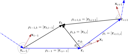
where and represents the position of -th agent relative to the -th agent (see Fig 1).
Using these recently introduced scalar shape variables, the consistency conditions (8) can be expressed as
| (12) | |||
| (13) |
for . In a similar way, the cycle closure constraint (7) can be expressed as
| (14) | |||
| (15) |
In actuality, certain simplifications allow us to consider only a subset of these variables and constraints. First, it is clear that for a particular choice of , (12) provides an explicit representation for the scalar shape variables , in terms of other shape variables, and therefore we can disregard those variables as well as constraint (12) from the following analysis. Furthermore, the choice of beacon frame is arbitrary and the proposed feedback law (see Section III) is invariant to any rotation of the beacon frame, and therefore there exists an symmetry enabling us to exclude from further analysis. Finally, one can show that (13) together with (14) and (15) can be expressed more concisely as simply (13) (holding for ) with (14). Therefore, the shape space can be parametrized by the scalar variables , for , subject only to the positivity constraints on and (necessary for the well-posedness of a feedback law introduced in the next section) and the constraints (13) - (14) for , i.e.
| (16) | |||
| (17) |
3 A beacon-referenced CB pursuit law
In this section we introduce a modified version of the CB pursuit law from [8] that introduces an additional term referenced to the beacon bearing. We construct this feedback law as a convex combination of two fundamental building blocks, expressed as
| (19) |
where is given by the original CB pursuit law [8] referenced to agent , and represents the deviation from a desired bearing angle to the beacon. More specifically, we choose
| (20) |
with being a control gain and the angle representing the desired offset between the -th agent’s heading and the current location of the -th agent. For the beacon tracking component, we let
| (21) |
where is the corresponding control gain and the angle is the desired offset between the current heading of the -th agent and the bearing to the beacon location. Note that the neighbor tracking goal may conflict with the beacon referencing goal, and the parameter maintains a balance between the beacon’s influence and the influence of the neighboring agent . In particular, for , is simply the original CB pursuit law with no reference to the beacon.
In terms of scalar shape variables, the feedback law can be expressed as
| (22) |
Remark 3.1.
As noted in [8], the last component of this feedback law (22) can be interpreted as the angular speed at which the baseline between agent- and agent- is rotating around the -th agent. Therefore it is plausible to evaluate the steering command without explicit measurement of distance between the agents, although it will require an appropriate sensing mechanism (mimicking the principle of compound eyes in visual insects).
Before going into detailed analysis of relative equilibria, we introduce the following simplifying assumptions:
-
(A1)
The speed of the agents are equal and constant. Hence, without loss of generality, we can assume for every .
-
(A2)
The controller gains ( and ) are equal and common for all agents, i.e. for every .
-
(A3)
The bearing angles () with respect to the beacon are common for all agents, i.e. for every .
Under assumptions (A1)-(A3), the closed loop shape dynamics ((18) with (22)) can be expressed as
| (23) | ||||
4 Relative equilibria
In this section we analyze the closed loop shape dynamics (23) to determine existence conditions and characterization of their equilibria (i.e. relative equilibria for the full dynamics (1) with (19)). At the extreme value of , the shape dynamics simplify to the cyclic CB pursuit dynamics previously analyzed in [2], while at the other extreme, inter-agent interaction is completely lost whenever . Therefore we restrict to lie in the open interval for the rest of our analysis.
From the form of and in (23), we can obtain necessary conditions at equilibrium given by
| (24) |
for . Similarly, by setting the dynamics of and equal to zero, we obtain (for )
| (25) | ||||
| (26) |
A straightforward calculation reveals that if with , then (26) results in a contradiction since its left hand side vanishes to zero, contrary to a non-zero () right hand side. Thus, at a relative equilibrium, we have
| (27) |
By introducing a new variable defined as
| (28) |
we obtain the following condition
| (29) |
from (25). This condition, along with (26), gives rise to
| (30) |
which in turn yields the equilibrium values of as
| (31) |
Now setting the dynamics of to zero, we obtain
| (32) |
for . As and at a relative equilibrium, (32) yields an equilibrium value for given by
| (33) |
Similarly, by (26) an equilibrium value of can be expressed as
| (34) |
As we have shown earlier in (29) that for every , it follows from (34) that the agents will be equi-distant from the beacon at any relative equilibrium. Hence, all relative equilibria for the system must be circling equilibria. Moreover, as both and are required to be positive, we have necessary conditions for existence of circling equilibrium, given by
| (35) | ||||
| and, | (36) |
4.1 Evaluating solutions for
It is easy to check that at any (circling) equilibrium of the closed loop shape dynamics, (29) with (32) implies that
| (37) |
for which we have two possible solutions given by
| (38a) | |||||
| (38b) |
where . Equilibrium values for can therefore be derived from (38a)-(38b), along with shape variable constraints (16)-(17) and positivity conditions (35)-(36).
If we let be the angle satisfying at equilibrium, then by (38a)-(38b) must assume either or . This aspect of binary possibilities holds true for every agent and therefore results in the branching depicted in Fig 2. This figure provides a graphical illustration of all possible solutions for (37), with each branch representing a candidate solution for . By considering a particular branch of the tree with (where ) copies of and copies of , we have
| (39) |
Now we focus on the shape variable constraints (16)-(17) to obtain solutions for . It is easy to check that the consistency conditions (17) hold true at any relative equilibrium of the closed loop dynamics. Additionally, by exploiting the relationship between equilibrium values of and , the cycle closure constraint (16) can be expressed as
| (40) |
where is the set of integers. By substituting (40) into (39), we have
| (41) |
We summarize the preceding discussion in the following proposition.
Proposition 4.1.
Consider an -agent cyclic CB pursuit system with beacon, whose shape dynamics is governed by (23) parametrized by , and the CB parameters . The following statements are true.
-
(a)
The only possible relative equilibria are circling equilibria.
-
(b)
Whenever , a circling equilibrium exists if and only if there exists and such that
-
(i)
the cardinality of the subset satisfies
(42) and
-
(ii)
(43) where is given by
(44)
At equilibrium, we have either or and the equilibrium values of , , and given by
-
(i)
Proof.
The first statement of the proposition directly follows from (34).
The preceding discussion has demonstrated that if a circling equilibrium exists, then and must satisfy (31),(35)-(36), (38a)-(38b), and (40), and the equilibrium values for , and can be expressed in terms of and by (27), (33), and (34). Further analysis of (35)-(36) demonstrated that if we let denotes the angle difference , then for each , we have one of two possibilities - either or , which we represent by the binary tree in Fig 2.
We now consider a particular branch of the binary tree (Fig 2), for which for exactly agents () and for the remaining agents. Clearly, for the first set of agents we have , while the remaining agents will have , and therefore there exists some such that for every , and the cardinality of the set is . This implies that (41) will hold (as demonstrated in the previous discussion), and thus for , it is clear that the positivity conditions (35)-(36) can be expressed as (43), with (44) following from (41) as long as .
It remains to be shown that (43) also encompasses the case , so that (43) is equivalent to (35)-(36). For , the positivity conditions (35)-(36) simplify to
| (45) | ||||
and we must show that there exists such that (43) with substituted into (44) is equivalent to (45). Choosing yields the desired result, and therefore statement (b) of the proposition is established. The characterization of the associated equilibrium values follows from the preceding discussion, and also establishes the sufficiency of our existence conditions, completing the proof. ∎
Remark 4.2.
The possibility of having cannot be ruled out for an even number of agents, in which case (41) can only be satisfied if is an integer multiple of . This case corresponds to existence of a continuum of circling equilibria.
Remark 4.3.
Letting denote the angular separation between agent and at a circling equilibrium, we have
| (46) |
Therefore the equilibrium value of angular separation between agent and agent is .
5 Stability analysis for the two-agent system
Here we consider the case where and analyze the stability of the associated circling equilibria. For the two-agent system, our constraints (16)-(17) imply that and for . Thus the dynamics (23) simplify for the two-agent case to
| (48) | ||||
and are subject to the constraint (16) which simplifies to
| (49) |
5.1 Existence of circling equilibria for the two-agent case
For the two-agent system, we have only two possible branches in Fig 2. The right-hand branch corresponds to , for which we have , and Proposition 4.1 does not apply. However, if for some , then a continuum of equilibria exist with and satisfying .
For the left-hand branch in Fig 2, we have (i.e. ) and therefore we can apply Proposition 4.1 (as long as ) for which (44) simplifies to
| (50) |
Thus we have (for )
| (51) |
and the second constraint in (43) requires . We label these options as Type 1 and Type 2 two-agent circling equilibrium and summarize the resulting characterization in Table 1, where we have made use of the notation
| (52) |
5.2 Stability analysis
We analyze the stability of two-agent circling equilibria by linearizing the dynamics (5) about the equilibria described in the previous section. Following the line of thought from the stability analysis in [3], we first demonstrate that the linearized dynamics will always have exactly one pair of pure imaginary eigenvalues resulting from the constraint equation (49).
First, denoting and the corresponding dynamics (5) by , we express (49) in terms of scalar constraints by
We define the manifold on which these constraints are satisfied by
| (53) |
which can be shown to be invariant under the dynamics (5). If we let denote a representative circling equilibrium for the two-agent case and let denote the linearization of the dynamics (49) about , then it was demonstrated in [3] that invariance of implies existence of a change of basis which will transform into upper-triangular form with a lower-right hand block. A suitable explicit form for the change of basis is given by , where
| (54) |
We note that the corresponding equilibrium will have ’s for the last two components.
By a straightforward calculation, we have
| (55) |
from whence it follows that, under the change of basis, the dynamics linearized about take the upper-triangular form
| (58) |
with
| (61) | ||||
| (64) |
where . It is clear from (61) that has a pair of pure imaginary eigenvalues at (resulting from the constraint equation (49)). By analogy with the argument presented in [3], we focus our stability characterization on the remaining five eigenvalues.
Returning to the original coordinates , we proceed with our stability analysis by linearizing the dynamics about the Type 1 CCW circling equilibrium from Table 1. One can show that the corresponding characteristic polynomial is given by
| (65) |
where
| (66) |
As expected based on the previous discussion, has two pure imaginary roots at . It is also clear that the roots of the quadratic term will have strictly negative real part if and only if . By the Routh-Hurwitz criterion, the roots of the cubic factor will be in the open left-half plane if and only if , , and . Since this last condition simplifies to , which always holds if , our requirement for stability is given by and .
A similar analysis of the other possible circling equilibria (i.e. Type 1 CW and Type 2 CCW and CW) results in analogous stability conditions, which can be summarized in the following proposition.
Proposition 5.1.
The Jacobian associated with the two-agent circling equilibria has two pure imaginary eigenvalues resulting from the constraint equation (49). The remaining eigenvalues all have real parts less than zero if and only if
-
•
and in the Type 1 CCW case;
-
•
and in the Type 1 CW case;
-
•
and in the Type 2 CCW case;
-
•
and in the Type 2 CW case.
Proof.
Follows from the discussion above. ∎
Note that these results are also summarized in Table 1.
Type 1 Type 2
6 Implementation Results
6.1 Experimental setup
We use Pioneer 3 DX (from Adept MobileRobots), a compact differential-drive mobile robot with reversible DC motors, high-resolution motion encoders, as the experimental platform. Onboard computation is done via 32-bit Renesas SH2-7144 RISC microprocessor, including the P3-SH microcontroller with ARCOS. ARIA, a software library from the developer, provides an interface for controlling and receiving data from the robot, and communication with the robot for sending control commands (forward velocity and turning rate) is carried out via 802.11-b/g/n networking.

Algorithm implementation (i.e, feedback law computation) has been carried out in C++ using ROS (Robot Operating System), along with ROS-ARIA, as the interfacing robotics middleware. The experiments have been carried out in a laboratory environment equipped with a sub-millimeter accurate Vicon motion capture system (www.vicon.com). The Dell workstation, which we use to evaluate control commands at , is connected to the Vicon server via a dedicated Ethernet connection.
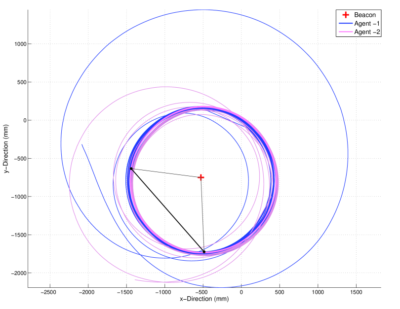
6.2 Two robots with asymmetric distribution on the circle
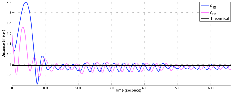
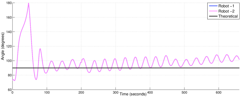
The first experiment presented here involves two robots circling around the beacon in a counter-clockwise direction. The parameters and were selected as and , respectively. These choices, by yielding the equilibrium value of angular separation as , demonstrate that the proposed approach can give rise to asymmetric distribution of agents on the circle (at equilibrium). Moreover, the parameter values and yield the circling radius as
and by choosing we get . The corresponding robot trajectories are shown in Fig 4(a), and the evolution of distance and angular separation for the agents are shown in Fig 4(b) and Fig 4(c), respectively (refer [13] for implementation videos). These figures show a quick convergence to the circling equilibrium (within ).
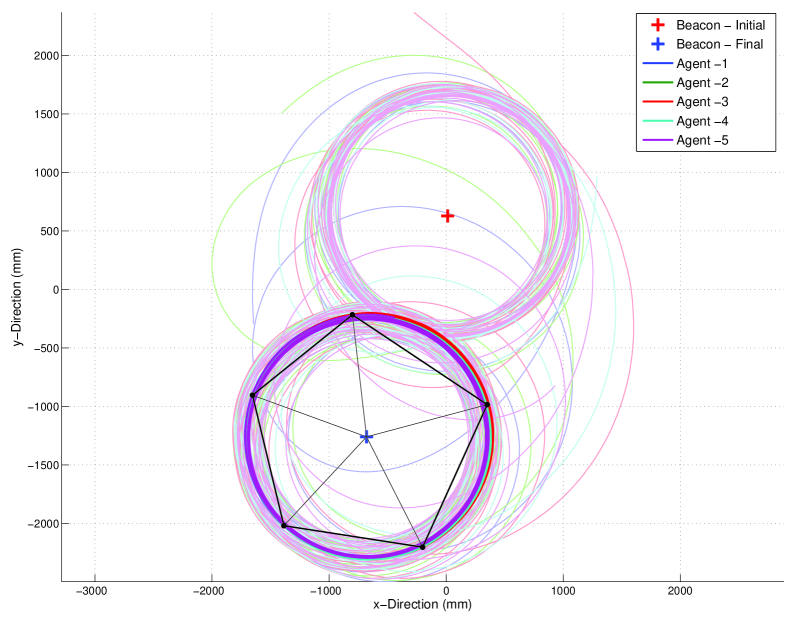


6.3 Five robots with symmetric distribution on the circle
Next we choose control parameters which result in five robots circling around the beacon in a clockwise direction, with the robots distributed symmetrically around the circle. More specifically, we choose the same value for every (), and let and . Then we have
and a choice of yields an equilibrium circle radius of . The corresponding robot trajectories, along with the evolution of distance and angular separation of the agents, are shown in Fig 5 (refer [13] for implementation videos). In this experiment we introduced a perturbation to the system at into the experiment, and later (at ) the beacon has been moved to a new position. In both cases, the formation quickly converges back to the desired circling equilibrium.
6.4 Discussion
The results show some level of imperfection during implementation of the proposed feedback law. This deviation from theoretical predictions can be attributed to multiple factors. To start with, our theoretical analysis assumes the agents to be point particles where in reality they occupy significant space (width - , swing radius - ). Also the placement of markers (necessary for measurement using Vicon motion capture system) introduces some error due to misalignment between center of the robot axle and origin of the body fixed frame. Furthermore, as only planar components of positions and heading were considered in measuring relevant quantities, a small slope (which has later been verified) in the lab floor acts as another source of error. However, in spite of these multiple sources of error, the proposed feedback mechanism (22) is able to restrict the error margins well below the physical dimension of the agents.
7 Conclusion and Future Work
We have introduced a modified version of the CB pursuit law which references a fixed beacon as well as a neighboring agent, and demonstrated that implementation in a cycle graph (with “spokes”) yields an interesting set of closed-loop dynamics. Analysis of those dynamics reveals the existence of circling equilibria centered on the beacon, and it is of particular interest that a specific equilibrium radius emerges as a function of the control parameters. Future work will focus on extending our analysis to the 3-d setting, as well as consideration of scenarios with multiple beacons or slowly moving beacons.
Acknowledgments
The authors would like to take this opportunity to thank P. S. Krishnaprasad and E. W. Justh for their valuable feedback and comments. They also appreciate the assistance from U. Halder in implementing the control law on mobile robots.
References
- [1] K. S. Galloway, E. Justh, and P. S. Krishnaprasad, “Portraits of cyclic pursuit,” in Proceedings of 50th IEEE Conference on Decision and Control and European Control Conference (CDC-ECC), Orlando, Florida, 2011, pp. 2724–2731.
- [2] K. S. Galloway, E. W. Justh, and P. S. Krishnaprasad, “Symmetry and reduction in collectives: cyclic pursuit strategies,” Proceedings of the Royal Society A: Mathematical, Physical and Engineering Science, vol. 469, no. 2158, 2013.
- [3] J. A. Marshall, M. E. Broucke, and B. A. Francis, “Formations of vehicles in cyclic pursuit,” IEEE Transactions on Automatic Control, vol. 49, no. 11, pp. 246–251, 2004.
- [4] T.-H. Kim and T. Sugie, “Cooperative Control for Target-Capturing Task Based on a Cyclic Pursuit Strategy,” Automatica, vol. 43, no. 8, pp. 1426 – 1431, 2007.
- [5] S. L. Smith, M. E. Broucke, and B. A. Francis, “A Hierarchical Cyclic Pursuit Scheme for Vehicle Networks,” Automatica, vol. 41, no. 6, pp. 1045 – 1053, 2005.
- [6] J. A. Marshall, M. E. Broucke, and B. A. Francis, “Pursuit Formations of Unicycles,” Automatica, vol. 42, no. 1, pp. 3 – 12, 2006.
- [7] J. Ramirez, M. Pavone, E. Frazzoli, and D. Miller, “Distributed Control of Spacecraft Formation via Cyclic Pursuit: Theory and Experiments,” in Proceedings of the American Control Conference (ACC), June 2009, pp. 4811–4817.
- [8] E. Wei, E. W. Justh, and P. S. Krishnaprasad, “Pursuit and an evolutionary game,” Proceedings of the Royal Society A: Mathematical, Physical and Engineering Science, vol. 465, no. 2105, pp. 1539–1559, 2009.
- [9] T. D. Seeley, S. Camazine, and J. Sneyd, “Collective decision-making in honey bees: how colonies choose among nectar sources,” Behavioral Ecology and Sociobiology, vol. 28, no. 4, pp. 277–290, 1991.
- [10] E. Justh and P. S. Krishnaprasad, “Steering laws and continuum models for planar formations,” in Proceedings of 42nd IEEE Conference on Decision and Control (CDC), Maui, Hawaii, 2003, pp. 3609–3615.
- [11] E. W. Justh and P. S. Krishnaprasad, “Equilibria and steering laws for planar formations,” Systems & Control Letters, vol. 52, no. 1, pp. 25 – 38, 2004.
- [12] R. L. Bishop, “There is more than one way to frame a curve,” The American Mathematical Monthly, vol. 82, no. 3, pp. 246–251, 1975.
- [13] Implementation Videos. [Online]. Available: http://ter.ps/beaconcb