Statistical inference for generalized Ornstein-Uhlenbeck processes
Abstract
In this paper, we consider the problem of statistical inference for generalized Ornstein-Uhlenbeck processes of the type
where is a Lévy process. Our primal goal is to estimate the characteristics of the Lévy process from the low-frequency observations of the process . We present a novel approach towards estimating the Lévy triplet of which is based on the Mellin transform technique. It is shown that the resulting estimates attain optimal minimax convergence rates. The suggested algorithms are illustrated by numerical simulations.
keywords:
T1 The financial support from the Government of the Russian Federation within the framework of the implementation of the 5-100 Programme Roadmap of the National Research University Higher School of Economics is acknowledged.
1 Introduction
Let be a Lévy process with a Lévy triplet . The main object of our study is the so-called generalized Ornstein-Uhlenbeck (GOU) process defined as
| (1) |
The GOU processes have recently got much attention in the literature. A comprehensive study of the GOU processes and an extended list of references can be found in the theses of Behme [2], where, in particular, it is shown that satisfies the following SDE:
The popularity of GOU processes is related to the fact they appear to be useful in several applications. For instance, the process (1) determines the volatility process in the COGARCH (COntinious Generalized AutoRegressive Conditionally Heteroscedastic) model introduced in Klüppelberg et al. [18]. One important result from the theory of GOU processes is that, under some conditions, the process (1) is stationary with invariant stationary distribution given by the distribution of the following exponential functional of
| (2) |
In fact, the properties of the functional (2) have been widely studied in the literature and we refer to the survey by Bertoin and Yor [7] for a theoretical background of the exponential functionals. In particular, it is known that the Mellin transform of the density of exponential functional,
satisfies the following recursive formula
| (3) |
where is a Laplace exponent of the process , i.e., and complex is taken from the strip
| (4) |
The recursive formula (3) first appeared for real in the paper by Maulik and Zwart [25]. The validity of (3) for complex was recently shown by Kuznetsov, Pardo and Savov [20]. If is a subordinator, the parameter is equal to infinity. Let us note that the functional appeared in such application areas as finance (see, e.g. the monograph by Yor [33]), carousel systems (see Litvak and Adan [23], Litvak and van Zwet [24]), self-similar fragmentations (see Bertoin and Yor [7]), and information transmission problems (especially TCP/IP protocol, see Guillemin, Robert and Zwart [13]). For the detailed discussion on the physical interpretations, we refer to Comtet, Monthus and Yor [10] and the dissertation by Monthus [26].
In this paper, we mainly focus on the case when is a subordinator with finite Lévy measure. In terms of the Lévy triplet , this means that , , and moreover . Suppose that the process (1) is observed at equidistant time points . Since under some mild assumptions the process is stationary and the invariant distribution is given by the distribution of the exponential functional (see Fasen, [12]), we assume that are also distributed as . Our main goal is statistical inference on the Lévy triplet based on the observations . More precisely, we will pursue the following two aims: (1) estimation of the drift term and the intensity parameter ; (2) estimation of the Lévy measure .
To the best of our knowledge, the statistical inference for GOU processes of the form (1) from their low-frequency observations has not been yet studied in the literature. In fact the resulting statistical problem is quite challenging and needs careful treatment. Indeed, the only connection between the stationary distribution of a GOU process, which can be estimated from the data, and the parameters of the underlying Lévy process is given by the recurrent relation (3) which is rather implicit. The main idea of our procedure for estimating the parameters of the process can be described as follows. First, by making use of (3), we estimate the Laplace exponent at the points , where is fixed and varies on the equidistant grid between and (with and as ) Afterwards, we use the representation
| (5) |
where , and stands for the Fourier transform of the measure , i.e., Since as by the Riemann-Lebesgue lemma, upon taking real and imaginary parts of the left and right hand sides of (5), we are able to consequently estimate the parameters and . With no doubt, the second aim, a complete recovering of the Lévy measure is the most difficult task. Since the estimates of the parameters and are already obtained, we can estimate by (5) the Fourier transform of for from . The last step of this procedure, the estimation of the Lévy measure , is based on the regularised inverse Fourier transform formula.
The above estimation algorithm bears some similarity to the spectral estimation algorithm introduced by Belomestny and Reiss [4], [5]. Let us also mention that the problem of statistical inference for Lévy processes (or some their generalizations) observed at low frequency was the subject of many studies, see, e.g. Neumann and Reiß [27], Reiß [28], Kappus [16], Trabs [31] and Jongbloed et al. [15]. Note that the last reference deals with the Lévy-driven Ornstein-Uhlenbeck processes, which are not of the form (1).
The paper is organized as follows. In the next section, we formulate our main assumptions and give some examples. In Section 3, the main estimation algorithm is presented and discussed in details. Next, we analyze the convergence rates of the proposed algorithms in Section 4 and provide some numerical examples in Section 5. The proofs of our theoretical results are collected in Section 6.
2 Main setup
In this article, we study the class of subordinators with finite Lévy measures as possible choice for the Lévy process . In terms of the Lévy triplet , this means that
| (6) |
A detailed discussion of the subordination theory as well as various examples of such processes (Gamma, Poisson, tempered stable, inverse Gaussian, Meixner processes, etc.), are given in [1], [6], [11], [29], [30]. Note that in the case of subordinators, the truncation function in the Lévy-Khinchine formula can be omitted, that is, the characteristic exponent of is equal to
| (7) |
Later on, we also need the Laplace exponent of , which is defined as
Under the assumption (6) the Laplace exponent is given by
| (8) | |||||
| (9) |
Let us summarise the main properties of the functional in this case.
Proposition 2.1.
The random variable admits a bounded density and fulfills for all If , then a.s. Moreover, the following relation holds for
| (10) | |||||
where is the Mellin transform of
3 Estimation of the Lévy triplet
In the sequel, we suppose that we are given by the observations of the process (1) at the equidistant time points with for some . Assuming that the process is stationary (see [2], [12]), we get that the random variables have all the same distribution, which coincides with the distribution of .
The first step of our estimation procedure consists in the estimation the Laplace exponent for , where is fixed and varies. An estimator of can be obtained from the recursive formula (3) for the Mellin transform of . In [9], this formula is proved for real positive such that and . The case of complex is considered in [20], where one can also find some generalizations of the formula (3) to the integrals with respect to Brownian motion with drift. In particular, applying Theorem 2 from [20], we get that (3) holds for any . In the situation when is a subordinator, the set coincides with the positive half-plane (equivalently, the parameter is equal to infinity) due to
Motivated by (10), we first estimate the Mellin transform via its empirical counterpart
| (11) |
and then define an estimate of the Laplace exponent by
| (12) |
If the sequence has some mixing properties, then we can expect that in probability.
3.1 Estimation of and
Under our assumptions, the Laplace exponent of the Lévy process can be represented in the form:
| (13) |
where and . The general idea of the procedure described below is to estimate the Laplace exponent at the points with and then use the relation (13) for the estimation of parameters. By the Riemann-Lebesque lemma, as (see, e.g., [17]) and we conclude from (13) that is approximately (at least for large ) a linear function in with the slope and the intercept term . This observation suggests that a properly weighted least-squares approach can be applied to estimate and . Let be a sequence of positive real numbers and be a nonnegative weight function supported on Define a scaled weight function and introduce the estimators of the parameters and as the solution of the following optimization problem:
with defined in (12). The above optimisation problem admits an explicit solution given by
with and , where
Taking into account the definition of the weight function , we get also some equivalent representations of the estimators and
In practice, we need to replace the above integrals by sums. To this end, let the numbers constitute an equidistant grid on the set for some We estimate the Mellin transform for all and and so get the estimates of the Laplace exponent at the discrete points (see above). Now we define an estimate of the parameter via
| (14) | |||||
| (15) |
Afterwards, we estimate the parameter by
| (16) | |||||
| (17) |
The whole algorithm is described below.
[couleur=blue!15, logo=\bccrayon] Algorithm 1: Estimation of and
-
1.
Estimate the Mellin transform
Estimate the Laplace exponent
Estimate by
Estimate by
3.2 Estimation of the Lévy measure
As a result of Algorithm 1, we obtain the estimates and of the parameters and respectively. Based on (13), we first define an estimate for the Fourier transform of via
| (18) |
Next we estimate the measure by a regularised Fourier inversion formula
| (19) |
where is a regularizing symmetric kernel supported on . Note that with a slight abuse of notation, we use also for the density of the Lévy measure, and for an estimate of this density. In what follows, we also use the notation . The formal description of the algorithm is given below.
[couleur=blue!15, logo=\bccrayon] Algorithm 2: Estimation of
-
1-2
The first two steps coincide with ones of Algorithm 1.
-
3.
Estimate for by
for
-
4.
Estimate by
Remark 3.1.
It is a worth mentioning that the estimation Algorithms 1 and 2 can be applied to a more general situation when
| (20) |
where the process is a difference between two subordinators, i.e., , and and are the processes of finite variation with Lévy measures and concentrated on and respectively. In fact, in this case, the formula (13) still holds with
Therefore, the consequent estimation of , and the Fourier transform of the measure , as well as the estimation of are still possible.
4 Convergence
In order to analyse the convergence properties of the estimates and we need to further specify the class of Lévy processes
Definiton 4.1.
For and let denote the set of all Lévy triplets , such that is supported on and
| (21) |
where
Note that if (21) holds, then is -times (weakly) differentiable with
| (22) |
It turns out that the convergence rates of the estimates and crucially depend on the asymptotic behaviour of the Mellin transform of In order to specify this behaviour, let us fix some and introduce two classes of probability densities:
| (23) | |||||
| (24) |
where and for any density stands for the Mellin transform of Before we formulate the main convergence results, let us look at some examples.
Example 4.2.
Consider the class of Lévy processes with and the Lévy density of the form
with , , . First note that the assumption (6) obviously holds. Let us now check (21). We can apply the well-known Erdélyi lemma to derive
for any exponentially decaying and smooth function on , and some complex depending on . Therefore, we conclude that
where depends on . Hence for any , the condition (21) holds for some . Furthermore, taking into account the asymptotic behaviour of the Gamma function (see, e.g., formula 8.328 from [14]):
| (25) |
we derive
where are the roots of the equation
see [19]. Therefore, for any , we conclude that with any .
Example 4.3.
Next, we provide an example of a Lévy process with having a density from . Consider a subordinator with drift and the Lévy density
The exponential functional of the process has a density of the form
with some , see [9]. In other words, has the same distribution as , where the r.v. has the Beta distribution with parameters and . The Mellin transform of the function in the half-plane is hence given by
Using (25), we conclude that the Mellin transform of has a polynomial decay in this case. More precisely,
as and therefore .
Let us now formulate the main result concerning the convergence of the estimates and .
Theorem 4.4 (upper bounds for and ).
Let be a Lévy process with a triplet from . Suppose that the sequence is -mixing and strictly stationary. Denote the -mixing coefficients of the sequence by .
-
(i)
Assume that the density of belongs to with some and , and moreover
(26) Then the quadratic risks of the estimates and under the choice satisfy the following asymptotic relations
and
as
-
(ii)
If and
(27) then the choice
leads to the rates
Proof.
Proof is given in Section 6.1. ∎
In a similar way, we can establish the upper bounds for the risk of . In the theorem formulated below, the quality of the estimate is measured in terms of the mean integrated squared error (MISE)
Theorem 4.5 (upper bounds for ).
Let the assumptions of Theorem 4.4 be fulfilled and let be a kernel satisfying
| (28) |
with some
-
(i)
Assume that the density of belongs to with some and , and moreover
Then under the choice , the MISE of the estimator is bounded as follows:
-
(ii)
If the density of belongs to the class and
then under the choice
we have
Proof.
Proof is given in Section 6.2. ∎
The next theorem shows that the rates obtained in the previous theorem are optimal up to a logarithmic factor.
Theorem 4.6 (lower bounds for ).
Fix some and define
for any and any probability density Then for some , it holds
| (29) |
where the infimum is taken over all possible estimates of the function based on i.i.d. sample from the distribution of such that the Lévy triplet of belongs to
Proof.
Proof is given in Section 6.3. ∎
An important condition of Theorems 4.4 and 4.5 is (26), which means that the sequence is exponentially -mixing. Since -mixing coefficient between two sigma-algebras is larger than or equal to the corresponding -mixing coefficient, it is sufficient to show that is an exponentially -mixing sequence (see Section 1.1 from [8]). For the case of the GOU processes (1), the latter question was addressed in [12]. The sufficient conditions for exponential -mixing given in [12] are:
-
1.
the distribution of has a Pareto-like asymptotic behaviour, that is,
with some and
-
2.
there exist , and such that with given in (7), and
As it is proved in [22], both conditions are guaranteed by the positiveness of and the existence of a positive zero of the function . We refer also to [21] for some further results in this direction.
5 Simulation study
Example 1. Consider the subordinator with the Lévy density
| (30) |
Note that in this case, . Define a Lévy process
| (31) |
where is a Brownian motion. The Laplace exponent of is given by
| (32) |
In [9], it is shown that the exponential functional is finite for any and , and moreover the density function of satisfies the following differential equation
| (33) |
Some special cases are considered below:
-
1.
In the case (pure jump process), this equation has a solution
(34) and therefore , where is a Gamma distribution with shape parameter and rate .
-
2.
If (pure jump process with drift), then
(35) In this situation , where is a Beta - distribution.
- 3.
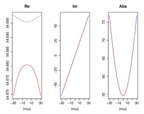
For our numerical study, we assume that the data are generated from the distribution of (2), where the process is defined by (31) with and the subordinator in the form (30) with , . A sample from the distribution of the integral can be simulated from the corresponding Beta-distribution, see (35). In the first step, we estimate the Mellin transform for with and and lying on the equidistant grid between and . Next, we estimate the Laplace exponent of by the formula (12). Figure 1 graphically compares the proposed estimator of the Laplace exponent with its theoretical values .
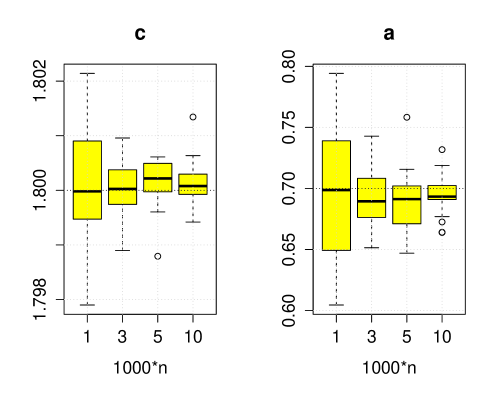
Estimates for the parameters and are given in (15) and (17), respectively. The boxplots of this estimates based on 25 simulation runs are presented on Figure 2.
Example 2. Consider the compound Poisson process
where is fixed, is a Poisson process with intensity and are i.i.d. random variables with a distribution . The integral admits the representation
where is the jump time of i.e., , and Note that if take only positive values, then is a subordinator. For the overview of the properties of the integral in the particular case (that is, is a Poisson process up to a constant), we refer to [7].
Fix some positive and consider the case when is the standard normal distribution truncated on the interval . The density function of is given by
where and are the density and the distribution functions of the standard Normal distribution. In this case, the Laplace exponent of is equal to
where the function can be calculated for complex arguments from the error function:
In this example, we aim to estimate the Lévy measure of the process , which is given by
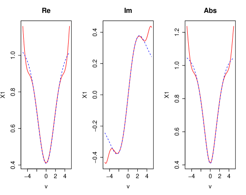
For our numerical study, we take , and . First, we estimate the Laplace exponent by (12). The quality of the corresponding estimate at the complex points with and can be visually seen in Figure 3.
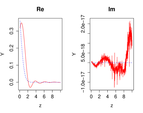
Next, we proceed with the estimation of the Fourier transform of the measure by applying (18). For the last step of the Algorithm 2, i.e. the reconstruction of the Lévy measure by (19), we follow [3] and use the so-called flat-top kernel, which is defined as follows:
The quality of the resulting estimate is shown in Figure 4.
6 Proofs
6.1 Upper bounds for the quadratic risks of and
The next proposition is the main technical result for this section.
Proposition 6.1.
Let be a Lévy triplet from . Suppose that the sequence of observations of the exponential functional is -mixing and strictly stationary. Denote the mixing coefficients of the sequence by .
Then for any we have
provided for some and the sequence satisfies
| (37) |
Proof.
1. Denote then
and we have
with
Note that
2. Since
we get
with
Following the lines of the proof of Theorem 1.5 from [8], we get
| (38) |
Note that the sum in the last representation converges as , because by Davydov’s inequality
| (39) |
and therefore the series is convergent if .
We have uniformly in As a result
The condition (37) implies now that Furthermore, we have
Similar to (38), we consider a representation
where . Applying once more Davydov’s inequality, we get
| (40) |
Now using the Cauchy-Schwarz inequality we get
Finally using the fact we derive
3. Turn now to the term By the Plancherel’s identity
∎
Proof of Theorem 4.4
-
(i)
Suppose that and then by taking for large enough, we arrive at
By taking we get
and
-
(ii)
Suppose that then by taking we get
Under the choice one derives
and
6.2 Upper bounds for
Proposition 6.2.
Proof.
6.3 Lower bounds for
Proof of Theorem 4.6. The general idea of the proof is to apply Theorem 2.7 from [32]. This theorem yields that (29) holds, if there exists a parameterized set of Lévy triplets
for some , and a set of parameters such that the following two properties hold.
-
(i)
For any ,
(41) -
(ii)
Denote by the probability distribution of the exponential Lévy model where is a Lévy subordinator with triplet Then
(42) for large enough, where stands for the Kullback-Leibler divergence between models, and .
Below we present a detailed proof for the polynomial case.
1. Presentation of the models. Consider an exponential Lévy model where is a Lévy subordinator with a triplet and for some It is clear that for some and the Laplace exponent of is given by
see Example 1 from Section 5. For the case of general classes with we could take a Lévy density of the form
Fix some and let us construct now a parameterized set of Lévy triplets with Lévy measure defined by
where small enough,
stands for the -th component of the vector , as , and
2. Distributional properties of the models. In this step, we perform some technical calculations, which will be used later. It holds
where is the Laplace transform of the function , which is equal to
We see that and
where is the Laplace exponent of a Lévy process with the Lévy triplet . Furthermore, the Laplace transform of is given by
with The Mellin transform of the density corresponding to the Lévy model satisfies the following functional equation
Since
and
we derive the following infinite product representation for the ratio
Furthermore, it can be proved that
for some absolute constant Note that the random variables with being a Lévy process with the triplet satisfies a.s. Moreover the density of the r.v. has the form
and the Mellin transform of is given by
| (43) |
see Example 4.3.
3. Class . In this step, we check that constructed models belong to class with and some . We have for any
The inequality for , where implies
where
It holds
provided for large enough Hence is bounded if
4. Upper bound for the -distance between elements of .
Fix two vectors We have
where
Consider, for example,
So we have
as and Analogously,
Furtheremore, one shows (see above) that
5. Choice of .
Our choice is based on the well-known Varshamov-Gilbert bound (see [32], Lemma 2.9), which implies that there are vectors such that
6. Upper bound for .
By Parseval identity for Mellin transforms, we get
So we get
where
The equation (43) implies that is finite for all with and
Hence
and the density of belongs to the class (see also Example 4.3). We have
and
Hence
| (44) |
for large .
7. Choice of . To complete the proof, we choose such that the conditions (41) and (42) are fulfilled. First note that since our model belongs to the class , we can take and see Step 3 of the proof for details. Second, comparing (44) with (42), we fix . This leads to the choice of as the solution of the equation
Combination of the results from Steps 4 and 5 yields the condition (41), because
for some and large enough. This observation completes the proof.
References
- [1] Barndorff-Nielsen, Ole E. and Shiryaev, A.N. Change of Time and Change of Measure. World Scientific, 2010.
- [2] Behme, A. Generalized Ornstein-Uhlenbeck process and extensions. PhD thesis, TU Braunschweig, 2011.
- [3] Belomestny, D. Statistical inference for time-changed Lévy processes via composite characteristic function estimation. The Annals of Statistics, 39(4):2205–2242, 2011.
- [4] Belomestny, D., and Reiss, M. Spectral calibration of exponential Lévy models. Fin. Stoch., 10:449–474, 2006.
- [5] Belomestny, D., and Reiss, M. Lévy matters IV. Estimation for discretly observed Lévy processes., chapter Estimation and calibration of Lévy models via Fourier methods, pages p. 1–76. Springer, 2015.
- [6] Bertoin, J. Lévy processes. Cambridge University Press, 1998.
- [7] Bertoin, J. and Yor, M. Exponential functional of Lévy processes. Probability Surveys, 2:191–212, 2005.
- [8] Bosq, D. Nonparametric statistics for stochastic processes. Estimation and prediction. Springer, 1996.
- [9] Carmona, P., Petit, F. and Yor, M. On the distribution and asymptotic results for exponential functionals of Lévy processes. In Exponential functionals and principal values related to Brownian motion, pages 73–130. Bibl. Rev. Mat. Iberoamericana, Madrid, 1997.
- [10] Comtet, A., Monthus, C., and Yor, M. Exponential functional of Brownain motion and disordered systems. J. Appl. Prob., 35(255-271), 1998.
- [11] Cont, R. and Tankov, P. Financial modelling with jump process. Chapman & Hall, CRC Press UK, 2004.
- [12] Fasen, V. Asymptotic results for sample autocovariance functions and extremes of integrated generalized Ornstein-Uhlenbeck processes. Bernoulli, 16(1):51–79, 2010.
- [13] Guillemin, F., Robert, P., and Zwart, B. AIMD algorithms and exponential functionals. The Annals of Applied Probability., 14(1):90–117, 2004.
- [14] Jeffrey, A., editor. Table of integrals, Series and Products. Academic Press, 7 edition, 2007.
- [15] Jongbloed, G., van der Meulen, F.H., van der Vaart, A.W. Nonparametric inference for Lévy driven Ornstein-Uhlenbeck processes. Bernoulli, 11(5):759–791, 2005.
- [16] Kappus, J. Adaptive nonparametric estimation for Lévy processes observed at low frequency. Stochastic Process. Appl., 124(1):730–758, 2014.
- [17] Kawata, T. Fourier analysis in probability theory. Academic Press, 1972.
- [18] Klüppelberg, C., Lindner, A., and Maller, R. A continuous-time GARCH process driven by a Lévy process: stationarity and second-order behaviour. J. Appl. Prob., 41:601–622, 2004.
- [19] Kuznetsov, A. On the distribution of exponential functionals for Lévy processes with jumps of rational transform. Stochastic Processes and their Applications, 122:654–663, 2012.
- [20] Kuznetsov, A., Pardo, J.C., and Savov, V. Distributional properties of exponential functionals of Lévy processes. Electronic Journal of Probability, 17(8):35 p., 2012.
- [21] Lee, O. Exponential ergodicity and -mixing property for Generalized Ornstein-Uhlenbeck processes. Theoretical Economics Letters, 2:21–25, 2012.
- [22] Lindner, A. and Maller, R. Lévy integrals and the stationarity of generalised Ornstein-Uhlenbeck process. Stochastic Processes and their Applications, 115(10):1701–1722, 2005.
- [23] Litvak, N. and Adan, I. The travel time in carousel systems under the nearest item heuristic. J. Appl. Prob., 38:45–54, 2001.
- [24] Litvak, N. and van Zwet, W. On the minimal travel time needed to collect items on a circle. J. Appl. Prob., 14(2):881–902, 2004.
- [25] Maulik, K. and Zwart, B. Tail asymptotics for exponential functionals of Lévy processes. Stochastic Process. Appl., 116:156–177, 2006.
- [26] Monthus, C. Etude de quelques fonctionnelles du mouvement Brownien et de certaines propriétés de la diffusion unidimensionnelle en milieu aléatoire. PhD thesis, Université Paris VI, 1995.
- [27] Neumann, M., and Reiss, M. Nonparametric estimation for Lévy processes from low-frequency observations. Bernoulli, 15(1):223–248, 2009.
- [28] Reiß, M. Testing the characteristics of a Lévy process. Stochastic Process. Appl., 123(7):2808–2828, 2013.
- [29] Sato, K. Lévy processes and infinitely divisible distributions. Cambridge University Press, Cambridge University Press, 1999.
- [30] Schoutens, W. Lévy processes in finance. John Wiley and Sons, 2003.
- [31] Trabs, M. Calibration of self-decomposable Lévy models. Bernoulli, 20(1):109–140, 2014.
- [32] Tsybakov, A. Introduction to nonparametric estimation. Springer, New York, 2009.
- [33] Yor, M. Exponential functional of Brownain motion and related processes. Springer., 2001.