Population Stability and Momentum

Abstract.

A new approach is developed to understand stability of a population and further understanding of population momentum. These ideas can be generalized to populations in ecology and biology.

Arni S.R. Srinivasa Rao^,,

(Appeared in Notices of the American Mathematical Society)

1. Introduction

One commonly prescribed approach for understanding the stability of system of dependent variables is that of Lyapunov. In a possible alternative approach - when variables in the system have momentum then that can trigger additional dynamics within the system causing the system to become unstable. In this study stability of population is defined in terms of elements in the set of births and elements in the set of deaths. Even though the cardinality of the former set has become equal to the cardinality of the latter set, the momentum with which this equality has occurred determines the status of the population to remain at stable. Such arguments also works for the other population ecology problems.

2. Population Stability Theory

Suppose $\left|P_{N}(t_{0})\right|$ be the cardinality of the set of people, $P_{N}(t_{0}),$ representing population at global level at time $t_{0}$, where $P_{N}(t_{0})=\left\{u_{1},u_{2},\cdots,u_{N}\right\}$, the elements $u_{1},u_{2},\cdots,u_{N}$ represent individuals in the population. Broadly speaking, the Lyapunov stability principles (see [VLL]) suggests, $\left|P_{N}(t_{0})\right|$ is asymptotically stable at population size $U$, if $\left|\left|P_{N}(T)\right|-U\right|<\epsilon$ ($\epsilon>0)$ at all $T$ whenever $T>t_{0}$. In some sense, $\left|P_{N}(t_{0})\right|$ attains the value $U$ over the period of time. Lotka-Voltera’s predator and prey population models provide one of the classical and earliest stability analyses of population biology (see for example, [JDM]) and Lyapunov stability principles often assist in the analysis of such models. These models have equations that describe the dynamics of at least two interacting populations with parameters describing interactions and natural growth. Outside human population models and ecology models, stability also plays a very important role in understanding epidemic spread [AR]. In this paper, we are interested in factors that cause dynamics in $P_{N}$ and relate these factors with status of stability. A set of people $P_{M}(t_{0})=\left\{u_{m_{1}},u_{m_{2}},\cdots,u_{m_{M}}\right\}$, where $P_{M}(t_{0})\subset P_{N}(t_{0})$, are responsible for increasing the population (reproduction) during the period $(t_{0},s)$ and contribute to $P_{N}(s)$, the set of people at $s$ (if they survive until the time $s$). The set $Q_{M_{1}}(s-t_{0})=\left\{v_{M_{11}},v_{M_{12}},\cdots,v_{M_{1M_{1}}}\right\}$ represent removals (due to deaths) from $P_{N}(t_{0})$ during the time interval $(t_{0},s)$. Let $\mbox{R}_{\phi}(s-t_{0})$ be the period reproductive rate (net) applied on $P_{M}(t_{0})$ for the period $(t_{0},s)$, then the number of new population added during $(t_{0},s)$ is $\mbox{R}_{\phi}(s-t_{0})\left|P_{M}(t_{0})\right|.$ Net reproduction rate at time $t_{0}$ (or in a year $t_{0}$) is the average number of female children that would be born to single women if she passes through age-specific fertility rates and age-specific mortality rates that are observed at $t_{0}$ (for the year $t_{0}$). Since net reproductive rates are futuristic measures, we use period (annual) reproductive rates for computing period (annual) increase in population. Let $\mbox{C}_{N_{1}}(s-t_{0})=\left\{w_{1},w_{2},\cdots,w_{N_{1}}\right\}$ be the set of newly added population during $(t_{0},s)$ to the set $P_{N}(t_{0}).$ After allowing the dynamics during $(t_{0},s)$, the population at $s$ will be

(2.1) $$P_{N}(t_{0})\cup C_{N_{1}}(s-t_{0})-Q_{M_{1}}(s-t_{0}) = \begin{cases}\left.\begin{array}[]{c}u:u\in P_{N}(t_{0})\cup C_{N_{1}}(s-t_{0})\mbox{ }\\ \mbox{and }u\notin Q_{M_{1}}(s-t_{0})\end{array}\right\}\end{cases}$$

$$= \left\{u_{1},u_{2},\cdots,u_{N+N_{1}-M_{1}}\right\}$$

Note that, $Q_{M_{1}}(s-t_{0})\subset P_{N}(t_{0})\cup C_{N_{1}}(s-t_{0})$, because the set of elements $\left\{v_{M_{1}},v_{M_{12}},\right.$ $\left.\cdots,v_{M_{1M_{1}}}\right\}$ eliminated during the time period $(t_{0},s)$ are part of the set of elements

$\left\{u_{1},u_{2},\cdots,u_{N},w_{1}\right.$ $\left.,w_{2},\cdots,w_{N_{1}}\right\}$ and the resulting elements surviving by the time $s$ are represented in equation (2.1). The element $u_{1}$ in the set (2.1) may not be the same individual in the set $P_{N}(t_{0})$. Since we wanted to retain the notation that represents people living at each time point, so for ordering purpose, we have used the symbol $u_{1}$ in the set (2.1).

Using Cantor–Bernstein–Schroeder theorem [PS], $\left|\mbox{C}_{N_{1}}(s-t_{0})\right|=$ $\left|Q_{M_{1}}(s-t_{0})\right|$ if $\left|\mbox{C}_{N_{1}}(s-t_{0})\right|$ $\leq$ $\left|Q_{M_{1}}(s-t_{0})\right|$ and $\left|\mbox{C}_{N_{1}}(s-t_{0})\right|$ $\geq\;$ $\left|Q_{M_{1}}(s-t_{0})\right|.$ If $\left|\mbox{C}_{N_{1}}(s-t_{0})\right|=$ $\left|Q_{M_{1}}(s-t_{0})\right|$ then the natural growth of the population (in a closed situation) is zero and if this situation continues further over the time then the population could be termed as stationary. Assuming these two quantities are not same at $t_{0}$, the process of two quantities $\left|\mbox{C}_{N_{1}}\right|$ and $\left|Q_{M_{1}}\right|$ becoming equal could eventually happen due to several sub-processes.

Case I: $\left|\mbox{C}_{N_{1}}\right|>$ $\left|Q_{M_{1}}\right|$ at time $t_{0}.$ We are interested in studying the conditions for the process $\left|\mbox{C}_{N_{1}}\right|\rightarrow$ $\left|Q_{M_{1}}\right|$ for some $s>t_{0}$. Two factors play a major role in determining the speed of this process, they are, compositions of the family of sets $\left[\left\{P_{M}(s)\right\}:\forall s>t_{0}\right]$ and $\left[\left\{\mbox{R}_{\phi}(s)\right\}:\forall s>t_{0}\right]$. Suppose $\left|P_{M}(s_{1})\right|>\left|P_{M}(s_{2})\right|>\cdots>\left|P_{M}(s_{T})\right|$ but the family of $\left\{\left|\mbox{R}_{\phi}(s)\right|\right\}$ does not follow any decreasing pattern for some $t_{0}<s_{1}<s_{2}<...<s_{T}<s$, then $\left|\mbox{C}_{N_{1}}\right|\nrightarrow\left|Q_{M_{1}}\right|$ by the time $s_{T}$. If $\mbox{R}_{\phi}(s_{1})>\mbox{R}_{\phi}(s_{2})>...>\mbox{R}_{\phi}(s_{T})$ for $t_{0}<s_{1}<s_{2}<...<s_{T}<s$ such that $\left|\mbox{R}_{\phi}(s_{T}-s_{T-1})\left|P_{M}(s_{T-1})\right|-Q_{M_{1}}(s_{T}-s_{T-1})\right|\rightarrow 0$ for some sufficiently large $T>t_{0}$ and sufficiently small $\left|\mbox{R}_{\phi}(s_{T}-s_{T-1})\right|$, then $\left|\mbox{C}_{N_{1}}\right|\rightarrow$ $\left|Q_{M_{1}}\right|$ by the time $s_{T}.$ Note that in an ideal demographic transition situation, both these quantities should decline over the period and the rate of decline of $\left|Q_{M_{1}}\right|$ is slower than the rate of decline in $\left|\mbox{C}_{N_{1}}\right|$ because $\left|\mbox{C}_{N_{1}}\right|>$ $\left|Q_{M_{1}}\right|$ at time $t_{0}.$ Demographic transition theory, in simple terms, is all about, determinants, consequences and speed of declining of high rates of fertility and mortality to low levels of fertility and mortality rates. For introduction of this concept see [KD] and for an update of recent works, see [JC]. Above trend of $\left|P_{M}(s_{1})\right|>\left|P_{M}(s_{2})\right|>\cdots>\left|P_{M}(s_{T})\right|$ (i.e. decline in people of reproductive ages over the time after $t_{0}$) happens when births continuously decrease for several years. Following the trend $\mbox{R}_{\phi}(s_{1})>\mbox{R}_{\phi}(s_{2})>...>\mbox{R}_{\phi}(s_{T})$ will lead to decline in new born babies and this will indirectly result in decline in rate of growth of people who have reproductive potential. However the decline in $\left|\mbox{R}_{\phi}(s)\right|$ for $s>t_{0}$ is well explained by social and biological factors, which need not follow any pre-determined mathematical model. However the trend in $\left|\mbox{R}_{\phi}(t)\right|$ for $t<t_{0}$ can be explained using models by fitting parameters obtained from data. During the entire process the value of $\left|Q_{M_{1}}\right|$ after time $t_{0}$ is assumed to be dynamic and decreases further. If a population continues to remain at this stage of replacement we call it a stable population. The cycle of births, population aging and deaths is a continuous process with discretely quantifiable factors. Due to improvement in medical sciences there could be some delay in deaths, but eventually the aged population has to be moved out of $\left\{P_{N}\right\}$, and consequently, population stability status can be broken with a continuous decline in $\left\{\left|C_{N_{1}}\right|\right\}$.

Case II: $\left|\mbox{C}_{N_{1}}\right|=$ $\left|Q_{M_{1}}\right|$ at time $t_{0}.$ It is important to ascertain whether this situation was immediately proceeded by case I or case II before determining the stability process. Suppose case II is immediately preceded by case I, then the rapidity and magnitude at which the difference between $\left|\mbox{C}_{N_{1}}\right|$ and $\left|Q_{M_{1}}\right|$ was shrunk prior to $t_{0}$ need to be quantified. Let us understand the contributing factors for the set $Q_{M}$. At each $t$, there is a possibility that the elements from the sets $C_{N_{1}}$, $P_{N}-C_{N_{1}}-P_{M}$, $P_{M}$ are contributing to the set $Q_{M}.$ Due to high infant mortality rates, the contribution of $C_{N_{1}}$ into $Q_{M}$ is considered to be high, deaths of adults of reproductive ages, $P_{M}$, and all other individuals (including the aged), $P_{N}-C_{N_{1}}-P_{M}$, will be contributing to the set $Q_{M}$. Case II could occur when $\left|\mbox{C}_{N_{1}}\right|$ and $\left|Q_{M_{1}}\right|$ are at higher values or at lower values. Equality at higher values possibly indicates, the number of deaths due to three factors mentioned here are high (including high old age deaths) and these are replaced by equal high number of births, i.e. $\left|R_{\phi}\right|$ and $\left|P_{M}\right|$ are usually high to reproduce a high birth numbers. If equality at lower values of $\left|\mbox{C}_{N_{1}}\right|$ and $\left|Q_{M_{1}}\right|$ occurs after phase of case I then the chance of $P_{N}$ remaining in stable position is higher. Suppose elements of $P_{N}$ are arbitrarily divided into $k-$independent and non-empty subsets, $A(1)$, $A(2)$, $\cdots$,$A(k)$ such that $\left|P_{N}\right|$$=$$\int_{1}^{k}\left|A(s)\right|ds$. Let $F$ be the family of all the sets $A(s)$ such that $\cup\left(A(s\right))=P_{N}$. Members of $F$ are disjoint. Suppose $\left(\begin{array}[]{c}F\\ k^{*}\end{array}\right)$ be an arbitrary size of $k^{*}$ of subset of $F$ are satisfying the case II and $F-\left(\begin{array}[]{c}F\\ k^{*}\end{array}\right)$ are not satisfying at time $t_{0}$ and $t>t_{0}$, then we are not sure of total population also attains stability by Theorem 1.

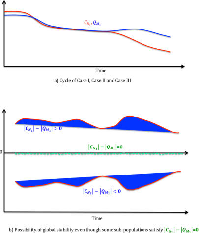
Figure 2.1. (a) The cycle of all the cases could follow one after another and the quantity at which equality of $C_{N_{1}}$ and $Q_{M_{1}}$ occurs determines the duration of the case II. (b) Some of the sub-populations which are not satisfied the equality of $C_{N_{1}}$ and $Q_{M_{1}}$ is compensated by the other sub-populations which are satisfying either $C_{N_{1}}>$ $Q_{M_{1}}$ or $C_{N_{1}}$ $<Q_{M_{1}}$.

Theorem 1.

Suppose each of the member of $\left(\begin{array}[]{c}F\\ k^{*}\end{array}\right)$ is satisfying the condition $\left|\mbox{C}_{N_{1}}\right|=$ $\left|Q_{M_{1}}\right|$ and $F-\left(\begin{array}[]{c}F\\ k^{*}\end{array}\right)$ are not satisfying the condition $\left|\mbox{C}_{N_{1}}\right|=$ $\left|Q_{M_{1}}\right|$ at time $t\geq t_{0}$, then this does not always leads $P_{N}$ to stability.

Proof.

Note that $F$ has collection of $k-$sets. Suppose a collection $C$ divides $C_{N_{1}}$ into $k-$components of subpopulations $\left\{C_{N_{1}}(1),C_{N_{1}}(2),\right.$ $\left.\cdots,C_{N_{1}}(k)\right\}$ such that $\left|C_{N_{1}}\right|$$=$$\int_{1}^{k}\left|C_{N_{1}}(s)\right|ds$, where $C_{N_{1}}(s)$ is the $s^{th}-$ subset in $C$ and a collection $Q$ divides $Q_{M_{1}}$ into $k-$ components of subpopulations $\left\{Q_{M_{1}}(1),Q_{M_{1}}(2),\cdots,Q_{M_{1}}(k)\right\}$ such that

$\left|Q_{M_{1}}\right|$ $\;=\;$$\int_{1}^{k}\left|C_{M_{1}}(s)\right|ds$, where $Q_{M_{1}}(s)$ is the $s^{th}-$subset in $Q$.

By hypothesis, $\left|C_{N_{1}}(s^{*})\right|=\left|Q_{M_{1}}(s^{*})\right|$ for $s^{*}\in$ $\left\{1^{*},2^{*},\cdots,k^{*}\right\}$ at each time $t\geq t_{0}$ until, say, $t_{T}$. The order between $k^{*}$ and $k-k^{*}$ could be one of the following: $2k^{*}<k$, $2k^{*}>k$, $k^{*}=\frac{k}{2}$. Suppose $C_{N_{1}}\subset C$ and $Q_{M_{1}}\subset Q$ with

$$C_{N_{1}}^{*} = \left\{C_{N_{1}}^{*}(1),C_{N_{1}}^{*}(2),\cdots,C_{N_{1}}^{*}(k)\right\}$$

$$Q_{M_{1}} = \left\{Q_{M_{1}}^{*}(1),Q_{M_{1}}^{*}(2),\cdots,Q_{M_{1}}^{*}(k)\right\}$$

for same above arbitrary combination of $k^{*}-$components and rest of the $k-k^{*}$ components are satisfying $\left|C_{N_{1}}^{**}(s^{**})\right|-\left|Q_{M_{1}}^{**}(s^{**})\right|\neq 0$ for all $s^{**}=1,2,\cdots,k-k^{*}$. We obtain unstable integral over all $k-k^{*}$ components to ascertain the magnitude of unstability.

(2.2) $$\int_{1}^{k-k^{*}}\left[\left|C_{N_{1}}^{**}(s^{**})\right|-\left|Q_{M_{1}}^{**}(s^{**})\right|\right]ds^{**}$$

The stable integral for this situation is

(2.3) $$\int_{1}^{k^{*}}\left[\left|C_{N_{1}}^{*}(s^{*})\right|-\left|Q_{M_{1}}^{*}(s^{*})\right|\right]ds^{*}$$

To check the unstable and stable points over the time period $(t_{0},t_{T})$, one can compute following integrals:

(2.4) $$\int_{t_{0}}^{t_{T}}\int_{1}^{k-k^{*}}\left[\left|C_{N_{1}}^{**}(s^{**})\right|-\left|Q_{M_{1}}^{**}(s^{**})\right|\right]ds^{**}du$$

(2.5) $$\int_{t_{0}}^{t_{T}}\int_{1}^{k^{*}}\left[\left|C_{N_{1}}^{*}(s^{*})\right|-\left|Q_{M_{1}}^{*}(s^{*})\right|\right]ds^{*}du$$

For each of the $k-k^{*}$ component, the values of $\left|C_{N_{1}}^{**}(s^{**})\right|-\left|Q_{M_{1}}^{**}(s^{**})\right|$ can be either positive or negative. If at time $t_{0}$, for all $s^{**}=1,2,\cdots,k-k^{*}$, the values of $\left|C_{N_{1}}^{**}(s^{**})\right|-\left|Q_{M_{1}}^{**}(s^{**})\right|$ are positive (or negative) then the eq. (2.2) will take a positive (or negative) quantity and the population at time $t_{0}$ is not stable. If such a situation continues for all $t_{T}\geq t_{0}$, then the integral in eq. (2.4) would never become zero and the population remains unstable in the entire period $(t_{0},t_{T})$. However, for some of the $s^{**}$, if the quantity $\left|C_{N_{1}}^{**}(s^{**})\right|-\left|Q_{M_{1}}^{**}(s^{**})\right|$ is positive and for other $s^{**}$, if the quantity $\left|C_{N_{1}}^{**}(s^{**})\right|-\left|Q_{M_{1}}^{**}(s^{**})\right|$ is negative such that eq. (2.2) is zero at each of the time points for the period $(t_{0},t_{T})$ then the population remains stable during this period (because by hypothesis the eq. (2.5) is zero). ∎

Case III. $\left|\mbox{C}_{N_{1}}\right|<$ $\left|Q_{M_{1}}\right|$ at time $t_{0}.$ Global occurrence of this case at lower values of $\left|\mbox{C}_{N_{1}}\right|$ and $\left|Q_{M_{1}}\right|$ indicates that the $P_{N}$ is declining and also is in unstable mode. $R_{\phi}$ has been very low consistently for the period $t<t_{0}$ and the supply to the set $P_{M}$ has diminished over a period in the past. All the subsets of $C_{N_{1}}$ and $Q_{M_{1}}$ might not be stable in case III, but by similar arguments of the Theorem 1, global population behavior nullifies some of the local population and case III is still satisfied globally.

All three cases would be repeated one following another. Most countries are currently facing case I with varying distance between $\left|\mbox{C}_{N_{1}}\right|$ and $\left|Q_{M_{1}}\right|$ .

3. Replacement Metric

We introduce a metric, $d_{M}$, which we call a replacement metric, with a space, $M_{r}$ as follows:

Definition 2.

(Replacement Metric).

Let $A_{1}=\min\left\{\left|\left|\mbox{C}_{N_{1}}(s)\right|-\left|Q_{M_{1}}(s)\right|\right|:s>t_{0}\right\}$ and

$A_{2}=\max\left\{\left|\left|\mbox{C}_{N_{1}}(s)\right|-\left|Q_{M_{1}}(s)\right|\right|:s>t_{0}\right\}$. Let $M_{r}=\left[A_{1},A_{2}\right]\subset\mathbb{R}^{+}$ and $M=\left\{\left|\left|\mbox{C}_{N_{1}}(s)\right|-\left|Q_{M_{1}}(s)\right|\right|\right.$ $\left.:s>t_{0}\right\}$ with the metric $d_{M}(x,y)=\frac{\left|x-y\right|}{2}$ . We can verify that $\left(M,d_{M}\right)$ is a metric space with $d_{M}:\left(M\times M\right)\rightarrow M_{r}$ and non-empty set $M.$

The metric $M$, in the definition 1 is bounded, because $d_{M}\left(x,y\right)<k$ for $k>0.$

Definition 3.

Suppose $\left|\left|\mbox{C}_{N_{1}}(s_{1})\right|-\left|Q_{M_{1}}(s_{1})\right|\right|=f_{1}$, $\left|\left|\mbox{C}_{N_{1}}(s_{2})\right|\right.$ $-$$\left.\left|Q_{M_{2}}(s_{2})\right|\right|=f_{2}$ and so on for $s_{1}<s_{2}<...$ . Then we say population is stable if $f_{s_{T}}\rightarrow 0$ for sufficiently large $T$ and $\frac{d}{ds_{T}}\left|\mbox{C}_{N_{1}}(s_{T})\right|=\frac{d}{ds_{T}}\left|\mbox{C}_{N_{1}}(s_{T})\right|=0$.

4. Conclusions

We can prove that the value at which the population remains stable is variable, i.e. the value at which the population becomes unstable by deviating from case II could be different from the value (at a future point in time) population becomes stable when it converges to case II. Replacement metrics (see definition 2) are helpful in seeing this argument and such analysis is not possible by Lotka-Voltera or Lyupunov methods. Due to population momentum, there will be an increase in the population even though the reproduction rate of the population becomes below the replacement level. Population stability will always attain a local stable points before diverging and again converging at a local stable point. The duration of a local stable point depends on the density of the population and resources available for the population.

References

[VLL]V. Lakshmikantham, X.Z. Liu (1993). Stability analysis
in terms of two measures. World Scientific Publishing Co., Inc., River
Edge, NJ.
[JDM]J.D. Murray (2003). Mathematical Biology I: An
Introduction. Springer-Verlag.
[AR]Arni S.R. Srinivasa Rao (2012). Understanding theoretically
the impact of reporting of disease cases in epidemiology. J. Theoret.
Biol. 302, 89–95.
[PS]P. Suppes (1960). Axiomatic set theory. The University
Series in Undergraduate Mathematics D. Van Nostrand Co., Inc.
[KD]K. Davis (1945). The World Demographic Transition,
Annals of the American Academy of Political and Social Science (237),
pp. 1–11.