Transient dynamics in the Anderson-Holstein model with interfacial screening

Abstract

We study the combined effects of electron-phonon coupling and dot-lead repulsion in the transport properties of the Anderson-Holstein model. We employ a recently proposed nonperturbative method to calculate the transient response of the system. By varying the initial conditions for the time propagation, we are able to disentangle two different dynamical processes, namely the local charge rearrangement due to the dot-lead contacting and the establishment of the nonequilbrium many-body state due to the application of the external bias. According to the distinct initial contacting, the current can exhibit transient oscillations of different nature. These origin from tunneling events that involve virtual Franck-Condon excitations, or virtual transitions between the resonant level and the Fermi energy of the leads.

I Introduction

The interplay of vibrational and electronic degrees of freedom during the charge tunneling through molecular junctions gives rise to striking nonequilibrium effectstroisi . These include phonon-assisted tunnelingphonass1 ; phonass2 , hysteresis-induced bistabilitybist1 ; bist2 ; bist3 , local heatingheat , molecular switchingswitch1 ; switch2 , and negative differential conductancephonass2 ; ndrexp1 ; ndrexp2 . Furthermore, if the electronic coupling to the vibrations is particularly strong a collective phenomenon known as Franck-Condon blockade (FCB) occursfcb . This manifests itself in a dramatic suppression of the tunneling current at low bias, accompanied by the appearance of several vibrational sidebands inside the Coulomb-blockade diamonds, recently observed in carbon nanotubes quantum dots (QD)vonoppen .

From the theoretical side, the quantitative description and understanding of the above phenomena represents a challenging nonequilibrium problem. Many observed properties can be addressed within the Anderson-Holstein modelwingreen , that describes a single electronic level coupled linearly to a vibrational mode and to metallic electrodes. Despite its apparent simplicity, however, this model does not allow for an analytic solution and approximate approaches must be resorted. Only very recently, numerically exact methods to calculate its nonequilibrium properties have been put forwardrabani ; albrecht ; wilner ; thossexact ; wilner2 . Beside providing a valuable validation of previous findings, the exact data have also revealed novel features, especially in the time domain, like the extraordinarily long-transient dynamics needed to reach the stationary state in the FCB regimealbrecht .

The inclusion of electron correlations widens the range of accessible phenomena, but at the same time complicates the theoretical treatment even further. While a considerable amount of work has been devoted to study intra-molecule electron-electron (e-e) interactionsreview (mainly to address the joint effects of vibrations and Coulomb blockade or Kondo-like correlations), the role of interfacial repulsion between the molecule and the leads has been explored only very recentlyperfetto1 . In that paper we developed a novel approach to study the complex interplay between the local electron-phonon (e-p) coupling together with the molecule-lead e-e repulsion. We showed that the exciton formation at the molecule-lead interface improves significantly the polaron mobility thus competing with the FCB. As a consequence the FCB regime is dynamically established after a long-lasting sequence of blocking-deblocking eventsalbrecht , characterized by exciton-enhanced current spikes.

In this paper we extend our previous study by computing the time-evolution of QD density under the application of an external bias, and by investigating how the transient current is modified by changing the initial conditions for the time propagation. When possible, we also compare our results with the exact data, finding very good agreement. We show that different ways of connecting in time the QD and the leads can produce qualitative differences in the transient current, accompanied by a change of the nature of the dominant oscillations.

II Model and formalism

The model we consider consists in a single-level QD attached to two semi-infinite one-dimensional noninteracting wires. An electron occupying the level is coupled to a single vibrational mode located in the QD, and at the same time interacts with the electrons in the leads which are in the proximity of the QD. The spinless Hamiltonian describing this system is given by (in standard notation)

$$\hat{H} = -t_{w}\sum_{\alpha,j=1}^{\infty}(\hat{d}^{\dagger}_{\alpha j}\hat{d}_{\alpha j+1}+\mathrm{h.c.})+T_{l}\sum_{\alpha}(\hat{d}^{{\dagger}}_{\alpha 1}\hat{d}+\mathrm{h.c.})$$ (1)

$$+ \epsilon_{d}\hat{n}_{d}+\omega_{0}\hat{a}^{\dagger}\hat{a}+\lambda\hat{n}_{d}(\hat{a}^{{\dagger}}+\hat{a})+U\hat{n}_{d}\sum_{\alpha}\hat{n}_{\alpha 1},\;\;\;\;$$

where $\alpha=L,R$ labels the Left and Right lead, and $\hat{n}_{d}=\hat{d}^{{\dagger}}\hat{d}$, $\hat{n}_{\alpha 0}=\hat{d}^{\dagger}_{\alpha 0}\hat{d}_{\alpha 0}$ are the densities on the QD and on the first sites of the lead $\alpha$ respectively. The system is perturbed by an external bias given by $\hat{H}_{V}=\sum_{\alpha}V_{\alpha}\hat{N}_{\alpha}$, with $\hat{N}_{\alpha}=\sum_{x}\hat{n}_{\alpha x}$ the total number of particles in wire $\alpha$ and $V=V_{L}-V_{R}$ the total applied voltage.

In the following we consider the continuum version $\hat{H}_{c}$ of the above model since it allows for a nonperturbative treatment of the e-e interaction via the bosonization techniquegiamarchi . To this end we first assume half-filled wide band leads with linear dispersion $\epsilon_{k}=v_{F}k$ (with $v_{F}=2t_{w}a$ the Fermi velocity and $a$ the lattice spacing) and constant tunneling amplitude $\Gamma=2\pi T_{l}^{2}\sum_{k}\delta(\omega-\epsilon_{k})=2T_{l}^{2}/t_{w}$, and then we unfold the left and right leadsboulat ; perfetto1 . In this way the first term of Eq. (1) takes the Dirac-like form $-\sum_{\alpha}iv_{F}\int dx\,\hat{\psi}^{\dagger}_{\alpha}(x)\partial_{x}\hat{\psi}_{\alpha}(x)$, where the electron field operator $\hat{\psi}_{\alpha}(x)$ describes an electron at position $x$ in the (chiral) lead $\alpha$ moving with velocity $v_{F}$. The rest of the continuum model is simply obtained by replacing $\hat{d}_{\alpha x}\to\hat{\psi}_{\alpha}(x)$, $\sum_{x}\to\int dx$, and by rescaling the model parameters according to $T_{l}\to t_{l}=2\sqrt{a}T_{l}$ and $U\to u=4aU$. We then bosonize the electron operators as giamarchi $\hat{\psi}_{\alpha}(x)=\frac{\eta_{\alpha}}{\sqrt{2\pi a}}e^{-2\sqrt{\pi}\,i\hat{\phi}_{\alpha}(x)},$ with boson field $\hat{\phi}_{\alpha}(x)=i\alpha\sum_{q>0}\zeta_{q}(\hat{b}^{\dagger}_{\alpha q}e^{-i\alpha qx}-\mathrm{h.c.})-\sqrt{\pi}x\hat{N}_{\alpha}/\mathcal{L}$, and $\eta_{\alpha}$ the anticommuting Klein factor. In the mode expansion of the boson field it holds $\zeta_{q}=\frac{e^{-\frac{av_{F}q}{2}}}{\sqrt{2\mathcal{L}q}}$, with $\mathcal{L}$ the length of the system. The electron density in the leads takes the form $\hat{n}_{\alpha}(x)=-\partial_{x}\hat{\phi}_{\alpha}(x)/\sqrt{\pi}$, and hence, up to an irrelevant termirlm , the bosonized continuum Hamiltonian readsnota

$$\hat{H}_{c} = \sum_{\alpha,q>0}v_{F}q\hat{b}^{\dagger}_{\alpha q}\hat{b}_{\alpha q}+\varepsilon_{d}\hat{n}_{d}+\omega_{0}\hat{a}^{\dagger}\hat{a}$$ (2)

$$+ t_{l}\sum_{\alpha}\left[\frac{\eta^{\dagger}_{\alpha}}{\sqrt{2\pi}}e^{-2\sqrt{\pi}\sum_{q>0}\zeta_{q}(\hat{b}^{\dagger}_{\alpha q}-\hat{b}_{\alpha q})}\hat{d}+\mathrm{h.c.}\right]$$

$$+ \hat{n}_{d}\left[\lambda(\hat{a}^{{\dagger}}+\hat{a})-u\sum_{\alpha,q>0}\frac{\zeta_{q}q}{\sqrt{\pi}}\,(\hat{b}^{\dagger}_{\alpha q}+\hat{b}_{\alpha q})\right].$$

Next we perform a multi-boson Lang-Firsov transformation to (formally) eliminate the e-p and e-p coupling appearing in the last line of the above equationirlm ; perfetto1 . The unitary operator $\hat{\mathcal{U}}=\mathrm{exp}[-\frac{\lambda}{\omega_{0}}(\hat{a}^{{\dagger}}-\hat{a})+2\sqrt{\pi}u\sum_{\alpha q}\frac{\zeta_{q}}{2\pi v}(\hat{b}^{\dagger}_{\alpha q}-\hat{b}_{\alpha q})]\hat{n}_{d}$ transforms the continuum Hamiltonian into $\hat{H}_{c}^{\prime}=\hat{\mathcal{U}}^{\dagger}\hat{H}_{c}\hat{\mathcal{U}}$ with (from now on all sums are over $q>0$)

$$\hat{H}_{c}^{\prime}=\sum_{\alpha q}v_{F}q\hat{b}^{\dagger}_{\alpha q}\hat{b}_{\alpha q}+\omega_{0}\hat{a}^{\dagger}\hat{a}+\tilde{\varepsilon}_{d}\hat{n}_{d}+t_{l}\sum_{\alpha}\left[\hat{f}^{{\dagger}}_{\alpha 0}\hat{d}+\mathrm{h.c.}\right].$$ (3)

In the transformed Hamiltonian it appears the renormalized fermion field

$$\hat{f}_{\alpha x}=\frac{\eta_{\alpha}}{\sqrt{2\pi a}}e^{-\frac{\lambda}{\omega_{0}}(\hat{a}^{{\dagger}}-\hat{a})+2\sqrt{\pi}\sum_{\beta q}\zeta_{q}W_{\alpha\beta}(\hat{b}^{\dagger}_{\beta q}e^{-iqx}-\hat{b}_{\beta q}e^{iqx})}$$ (4)

evaluated in $x=0$, with the effective interactions $W_{RR}=W_{LL}=1-u/(2\pi v_{F})$ and $W_{RL}=W_{LR}=-u/(2\pi v_{F})$, and renormalized energy level $\tilde{\varepsilon}_{d}=\varepsilon_{d}-\frac{\lambda^{2}}{\omega_{0}}-u^{2}\sum_{q}\frac{e^{-aq}}{\pi v_{F}\mathcal{L}}$. In the new basis we have a noninteracting QD coupled to effective leads (bosonic baths) whose ground state for $t_{l}=0$ is $|\Psi_{0}\rangle=|0_{p}\rangle\otimes\prod_{\alpha q}|0_{\alpha q}\rangle$, where $|0_{p}\rangle$ and $|0_{\alpha q}\rangle$ are the vacua of the boson operators $\hat{a}$ and $\hat{b}_{\alpha q}$ respectively; the tunneling coupling occurs via the correlated-polaron operator $\hat{f}$.

III Equation of motion

The great advantage of casting the Hamiltonian in the form of Eq. (3) is the possibility of writing an approximate equation of motion for the nonequilibrium QD Green’s function, solely in presence of a correlated-polaron embedding self-energy. The latter accounts for the presence of the biased leads as well as for the e-p and e-p interactions in a nonperturbative way. We define the QD Green’s function on the Keldysh contour as $G(z,z^{\prime})=\frac{1}{i}\langle{\cal T}{\hat{d}(z)\hat{d}^{{\dagger}}(z^{\prime})}\rangle,$ where ${\cal T}$ is the contour ordering, operators are in the Heisenberg picture with respect to $\hat{H}_{c}^{\prime}+\hat{H}_{B}$ (the bias perturbation does not change after the transformation); the average is taken over the uncontacted ground state $|\Psi_{0}\rangle\otimes|n_{d}\rangle$, $|n_{d}\rangle$ being the state of the QD with density $n_{d}$, with $n_{d}$ ranging from $0$ to $1$. In Ref. perfetto1, we proposed a controlled approximation scheme in order to derive a closed (and numerically solvable) equation of motion for $G$, that reads

$$(i\partial_{z}-\tilde{\varepsilon}_{d})G(z,z^{\prime})-\int_{\gamma}d\bar{z}\sum_{\alpha}\Sigma_{\alpha}(z,\bar{z})G(\bar{z},z^{\prime})=\delta(z,z^{\prime}),$$ (5)

where $\Sigma_{\alpha}(z,z^{\prime})$ is the correlated-polaron embedding self-energy. The real-time Keldysh components of $\Sigma$ can be evaluated exactly using again the bosonization methodgiamarchi and read

$$\Sigma^{\lessgtr}_{\alpha}(t,t^{\prime})=\pm\frac{iv_{F}\Gamma e^{-g}}{4\pi a^{1-\beta}}e^{i[\varphi_{\alpha}(t^{\prime})-\varphi_{\alpha}(t)]}\frac{e^{ge^{\pm i\omega_{0}(t-t^{\prime})}}}{[a\mp iv_{F}(t-t^{\prime})]^{\beta}},$$ (6)

with adimensional e-p coupling $g=(\lambda/\omega_{0})^{2}$, interaction dependent exponent $\beta=1+\frac{u(u-2\pi v_{F})}{2\pi^{2}v_{F}^{2}}$ and phase $\varphi_{\alpha}(t)=\int^{t}_{0}d\bar{t}\,V_{\alpha}(\bar{t})$. The power-law reflects the collective excitonic response of the lead electrons to the attractive potential due to the creation of a hole in the QDmahan . In the noncorrelated case we have $\beta=1$, while electron correlations produce $\beta<1$; the smaller the exponent is, the stronger is the exciton effect.

The integral in Eq. (5) runs over the Keldysh contour $\gamma$, and using the Langreth ruleskeldysh it is converted into a coupled system of Kadanoff-Baym equationsdvl.2007 ; mssvl.2009 (KBE) which we solve numerically. Once the Keldysh components of $G(z,z^{\prime})$ are known, the time-dependent QD density is calculated as $n(t)=-iG^{<}(t,t)$, while the transient current flowing through the QD and the $\alpha$ lead can be evaluated according to

$$I_{\alpha}(z)=\int_{\gamma}d\bar{z}\,\Sigma_{\alpha}(z,\bar{z})G(\bar{z},z)+\mathrm{h.c.}\quad$$ (7)

IV Initial conditions

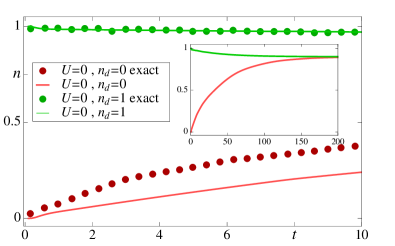
Figure 1: TD density in the partitioned approach for $U=0$ with initial QD occupancy $n_{d}=0$ (red) and $n_{d}=1$ (green). Exact data from Ref. albrecht, are also displayed (circles). The rest of parameters are $\lambda=16$, $\omega_{0}=8$, $V=26$, $\tilde{\epsilon}_{d}=-10$, $v_{F}/a=100$. Units: $\Gamma$ for energies and $\Gamma^{-1}$ for times. The insets displays the TD result for a longer propagation time, in order to appreciate that the two densities reach the same steady-state value.

Before presenting the explicit numerical results, a brief discussion about the initial conditions is in order. To solve practically Eq. (5), one has to set the initial value $G^{<}(0,0)=-in_{d}$, that corresponds to (apart from the $-i$ factor) the initial density in the QD. This means that our propagation scheme assumes the system initially uncontacted ($t_{l}=0$, i.e. the leads and the QD are in their ground states), and the contacts and bias are switched at time $t=0$. Therefore the subsequent transient regime accounts for two different dynamical processes: (i) the charge rearrangement due to the QD-lead contacting (creation of Friedel-like oscillations in the leads, etc), and (ii) the establishment of a genuine nonequilbrium many-body state due to external bias (the rise of the current towards its steady-state value, etc). This scheme corresponds to the so-called partitioned approach. However, in a more realistic situation, the bias is switched when the system is already contacted and in equilibrium (i.e. the leads and the QD are in the ground state with $t_{l}\neq 0$). This is the so-called partition-free approachcini ; stefalmb . Here the transient dynamics can be very different from the partitioned case, since the two processes (i) and (ii) described above are not superimposedperfspin ; perfspin2 ; perfgraph ; perfspin ; perfjosep ; riku . In our scheme we can numerically simulate the partition-free appraoch, since the bias function $V_{\alpha}(t)$ (appearing in the phase $\varphi_{\alpha}$ in Eq. (6)) is completely arbitrary. In practice we consider a step-like bias function $V_{\alpha}(t)=V_{\alpha}\theta(t_{th})$, that corresponds to take the system initially uncontacted with a given $n_{d}$ at time $t=0$, let the system thermalize (dynamics (i)) till a time $t_{th}$ at which no current flows across the links, and then we switch the bias perturbation on (dynamics (ii))gkba .

V Transient density

In Fig. 1 we assess the accuracy of the proposed approach by comparing our results against exact data availabale in the literature for $U=0$, and obtained within the partitioned schemealbrecht . It appears that the agreement is exceptionally good for initial density $n_{d}=1$, while for $n_{d}=0$ we predict a slower raise of the density towards its steady-state value. We recall, however, that in this case our results improve the state-of-the-artalbrecht . In the inset we show the TD density for a longer propagation time (not within reach of current numerical techniques), in order to appreciate that the two densities reach the same steady-state value, as it should be.

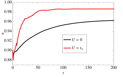
Figure 2: TD relaxation towards the equilibrium density for $U=0$ (black) and $U=t_{w}$ (red), with initial QD occupancy $n_{d}=0.9$ and bias $V=0$. The rest of parameters and units are the same as in Fig. 1.

We now study the effects induced by the QD-lead repulsion $U$. Fig. 2 displays the relaxation of the QD density from the uncontacted value ($n_{d}=0.9$) to the equilibrium value, after that the system has been contacted without bias. We see that the effect of the screening interaction is twofold: enhance the asymptotic value of $n(t)$, and speed up the relaxation time. The first effect origins from the fact that a finite electron density in the QD induces a charge depletion in the portion of the leads which are in the proximity of the interface; part of the repelled charge, in turn, migrates towards the QD thus enhancing its population. The second, instead, is a jamming effect reminiscent of the one found in Ref. irlm, , that is due to the dynamical screening of the QD charge and tends to stabilize faster the value of $n(t)$.

VI Transient current

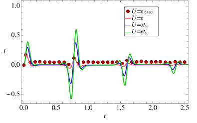
Figure 3: TD current within the partitioned scheme for different $U$, initial QD occupancy $n_{d}=1$, and bias voltage $V=5\Gamma$. For $U=0$, exact data from Ref. albrecht are also displayed (circles). The rest of parameters and units are the same as in Fig. 1.

In this section we study the TD current $I(t)=[I_{L}(t)+I_{R}(t)]/2$ flowing under the application of the external bias. As in the case of the density, the approach is first validated by comparing our results with the exact results recently obtained for $U=0$ within diagrammatic Monte Carlo simulationsalbrecht . In Fig. 3 a remarkable agreement between the two approaches (within the partitioned scheme) can be appreciated. In particular our method efficiently reproduces the very peculiar transient behavior of $I(t)$ before the steady-state is reached. In the absence of e-e interactions the time-dependent current displays quasi-stationary plateaus where almost no electron tunnels across the junction. At times $t_{n}=2n\pi/\omega_{0}$ a deblocking effect occurs, and the current exhibits narrow bumps, signaling a sudden electron flow. When the e-e interaction is considered, we observe a significant enhancement of the transport properties, characterized by larger current spikes. As we show below, the physical interpretation of such striking transient dynamics provides a clue to understand how the FCB regime is dynamically established, and how e-e interaction modify the FCB scenario. At $t=t_{n}$ an electron occupying the QD is in the polaron ground-state with phonon cloud centered at $x\sim n\lambda$ (with $n\approx 1$). At this time the polaron tunnels to the lead, causing a displacement of the oscillator to $x\to 0$ (since now $n=0$). At this point the polaron cannot hop back to the QD since the overlap between the two shifted oscillator wavefunctions is negligible. Only after a vibrational period $2\pi/\omega_{0}$ the overlap returns to be large, and the polaron can hop back to the QD. Let us now consider the effects of e-e interaction. The mechanism described above is modified as follows: If at time $t=t_{n}$ ane electron is on the QD, the electron density diminishes at the site of the lead boundary, thus overcoming the hopping suppression due to the Pauli principle and enhancing the effective tunneling rateborda ; goldstein ; irlm . Similarly, at time $t=t_{n+1}$ the electron can easily tunnel back to the QD, being attracted by the hole previously left. This explains in a transparent way the $U$-induced enhancement of the current spikes observed in Fig 3.

We now focus on the effects of the different initial conditions. To this end we compare the results obtained within the partitioned scheme vs the ones obtained within partition-free scheme. In Fig. 4 we plot the TD current in the two schemes without (upper panel) and with (lower panel) screening interaction $U$. For the partitioned scheme we employ two different initial values of the QD density, namely $n_{d}=1$ (red curve) and $n_{d}=0$ (blue curve). We recall that in order to display the partition-free curves together with the partitioned ones, we shift the former of $t_{th}$. We observe that the three currents correctly reach the same steady-state and do it via similar long-lasting sequences of current spikes, (typical of the FCB regime), and, as expected, the current in presence of $U$ is enhanced with respect to that calculated at $U=0$ (Coulomb deblocking). In this case the partitioning effects reflect in a quantitative change of the early transient current (see the black curves vs the red and blue ones), even though the qualitative FCB-like transient behavior does not change.

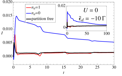
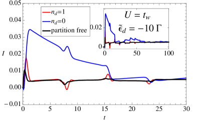
Figure 4: Comparison between TD currents within the partion-free scheme (black) vs partitioned scheme with $n_{d}=0$ (blue) and $n_{d}=1$ (red). $U=0$ in the upper panel and $U-t_{w}$ in the lower panel. The rest of parameters and units are the same as in Fig. 1. The insets display the TD result for a longer propagation time. The TD curve of the partition-free case has been shifted of $t_{th}=100$.

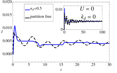
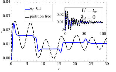
Figure 5: Comparison between TD currents in the resonant condition $\tilde{\varepsilon}_{d}=0$ within the partion-free scheme (dashed black) vs partitioned scheme with $n_{d}=0.5$ (blue). $U=0$ in the upper panel and $U=t_{w}$ in the lower panel. The rest of parameters and units are the same as in Fig. 1. The insets display the TD result for a longer propagation time. The TD curve of the partition-free case has been shifted of $t_{th}=100$.

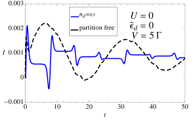
Figure 6: Comparison between TD currents in the resonant condition $\tilde{\varepsilon}_{d}=0$ within the partion-free scheme (dashed black) vs partitioned scheme with $n_{d}=0.5$ (blue). $U=0$ and bias $V=5\Gamma$. The rest of parameters and units are the same as in Fig. 1. The TD curve of the partition-free case has been shifted of $t_{th}=100$.

In order to magnify the partitioning effects, we focus on the perfect resonant case, obtained by setting $\tilde{\varepsilon}_{d}=0$. Here (see Fig. 5) the partition-free transient current displays qualitative differences. If we use $n_{d}=1/2$ for partitioned scheme, the TD density is pinned in both schemes at the constant value $n(t)=1/2$ at each time (not shown), due to symmetry constraints. Despite the TD density is identical in the two schemes, the TD currents are remarkably different. In particular the FCB pattern tends to disappear in the partition-free case, and the transient current has a smooth oscillating behavior with dominant frequency $V/2$, i.e the energy difference between the molecular level and the Fermi energy of the leads. Here the interaction $U$ (lower panel of Fig. 5) amplifies these oscillations, thus enhancing further the difference between the two currents. This behavior is confirmed by decreasing the bias from $V=26\Gamma$ to $V=5\Gamma$, as shown in Fig. 6. It is clear that the transient frequency of the partition-free current reduces according to the smaller value of $V$, whereas the spikes of the partitioned current continue to appear with periodicity given by the phonon frequency $\omega_{0}$.

This qualitative change can be interpreted as follows: At the resonance ($\tilde{\varepsilon}_{d}=0$) and if the leads are initially relaxed around the QD, the dressed tunneling (that involves the excitation of a phonons with energy $\omega_{0}$) has the same probability as the bare tunneling (that involves virtual transition between the QD and the Fermi level of the leads). In the partitioned case, instead, the bare tunneling is suppressed because the electron charge in the leads is optimally rearranged in the proximity of the QD.

VII Conclusions

We presented a systematic study of the time-dependent transport properties of the Anderson-Holstein model in presence of dot-lead screening interaction. Thanks to the analytic expression of the correlated-polaron embedding self-energy we gained a clear understanding of how the two interactions combine together. The validity of the approach was also corroborated by comparing our results against exact data available in the literature. Our approximated scheme allows for a calculation of the time-dependent density that improves the current state-of-the-art, and at the same incorporates the screening effects in a physically correct way. The transient behavior of the current was carefully analyzed by considering different initial contacting of the leads. We showed that at early times the current can exhibit qualitative different behaviors, depending if the electron liquid in the leads is relaxed or not around the QD before the switching of the bias. At resonance, we found that the partition-free current displays coherent oscillations with frequency equal to the applied bias, whereas the partitioned current has a periodicity dictated by the phonon frequency.

We acknowledge funding by MIUR FIRB grant No. RBFR12SW0J.

References

- (1) M. Galperin, M.A. Ratner, A. Nitzan, and A. Troisi, Science 319, 1056 (2008).
- (2) B. J. LeRoy, S. G. Lemay, J. Kong, and C. Dekker, Nature 432, 371 (2004).
- (3) S. Sapmaz, P. Jarillo-Herrero, Ya. M. Blanter, C. Dekker, and H. S. J. van der Zant, Phys. Rev. Lett. 96, 026801 (2006).
- (4) C. Li, D. Zhang, X. Liu, S. Han, T. Tang, C. Zhou, W. Fan, J. Koehne, J. Han, M. Meyyappan, et al., Appl. Phys. Lett. 82, 645 (2003).
- (5) E. Lörtscher, J. Ciszek, J. Tour, and H. Riel, Small 2, 973 (2006).
- (6) P. Liljeroth, J. Repp, and G. Meyer, Science 317, 1203 (2007).
- (7) Z. Huang, B. Xu, Y. Chen, M. Di Ventra, and N. Tao, Nano Lett. 6, 1240 (2006).
- (8) B. Y. Choi, S. J. Kahng, S. Kim, H. Kim, H. W. Kim, Y. J. Song, J. Ihm, and Y. Kuk, Phys. Rev. Lett. 96, 156106 (2006).
- (9) V. Meded, A. Bagrets, A. Arnold, and F. Evers, Small 5, 2218 (2009).
- (10) J. Gaudioso, L. J. Lauhon, and W. Ho, Phys. Rev. Lett. 85, 1918 (2000).
- (11) E. Pop, D. Mann, J. Cao, Q. Wang, K. Goodson, and H. Dai, Phys. Rev. Lett. 95, 155505 (2005).
- (12) J. Koch and F. J. von Oppen, Phys. Rev. Lett. 94, 206804 (2005).
- (13) R. Leturcq, C. Stampfer, K. Inderbitzin, L. Durrer, C. Hierold, E. Mariani, F. von Oppen and K. Ensslin, Nature Phys. 5, 327 (2009).
- (14) N. S. Wingreen, K. W. Jacobsen, and J. W. Wilkins, Phys. Rev. B 40, 11834 (1989).
- (15) L. Mühlbacher and E. Rabani, Phys. Rev. Lett. 100, 176403 (2008).
- (16) K. F. Albrecht, A. Martín-Rodero, R. C. Monreal, L. Mühlbacher, and A. Levy Yeyati, Phys. Rev. B 87, 085127 (2013).
- (17) E.Y. Wilner, H. Wang, G. Cohen, M. Thoss, E. Rabani, arXiv:1301.7681.
- (18) H. Wang and M. Thoss, J. Chem. Phys. 138, 134704 (2013).
- (19) E.Y. Wilner, H. Wang, M. Thoss, and E. Rabani, Phys. Rev. B 89, 205129 (2014).
- (20) For a recent review, see e.g. N.A. Zimbovskaya and M.R. Pederson, Phys. Rep. 509, 1 (2011), and references therein.
- (21) E. Perfetto and G. Stefanucci, Phys. Rev. B 88, 245437 (2013).
- (22) T. Giamarchi, Quantum Physics in One Dimension (Clarendon, Oxford, 2004).
- (23) E. Boulat, H. Saleur, and P. Schmitteckert, Phys. Rev. Lett. 101, 140601 (2008).
- (24) E. Perfetto, G. Stefanucci and M. Cini, Phys. Rev. B 85, 165437 (2012).
- (25) We remind that for the model threated within the wide-band-limit approximation and the model return exactly the same results, that, in turn, do not depend on , see e.g. Refs. psc.2010, ; irlm, ; ringlutt, .
- (26) E. Perfetto, G. Stefanucci and M. Cini, Phys. Rev. Lett. 105, 156802 (2010).
- (27) E. Perfetto, M. Cini, and S. Bellucci Phys. Rev. B 87, 035412 (2013).
- (28) G. D. Mahan, Phys. Rev. Lett. 18, 448 (1967); P. Nozières, C.T. De Dominicis, Phys. Rev. 178 1097 (1969).
- (29) G. Stefanucci and R. van Leeuwen, Nonequilibrium Many- Body Theory of Quantum Systems: A Modern Introduction (Cambridge University Press, 2013).
- (30) N. E. Dahlen and R. van Leeuwen, Phys. Rev. Lett. 98, 153004 (2007).
- (31) P. Myöhänen, A. Stan, G. Stefanucci and R. van Leeuwen, Phys. Rev. B 80, 115107 (2009).
- (32) M. Cini, Phys. Rev. B 22, 5887 (1980).
- (33) G. Stefanucci and C. O. Almbladh, Phys. Rev. B 69, 195318 (2004).
- (34) G. Stefanucci, E. Perfetto, and M. Cini, Phys. Rev. B 78, 075425 (2008).
- (35) E. Perfetto, G. Stefanucci, and M. Cini, Phys. Rev. B 78, 155301 (2008).
- (36) E. Perfetto, G. Stefanucci, and M. Cini, Phys. Rev. B 80, 205408 (2009).
- (37) G. Stefanucci, E. Perfetto, and M. Cini, Phys. Rev. B 81, 115446 (2010).
- (38) E. Perfetto, G. Stefanucci, and M. Cini, Phys. Rev. B 82, 035446 (2010).
- (39) R. Tuovinen, E. Perfetto, G. Stefanucci, R. van Leeuwen, Phys. Rev. B 89, 085131 (2014).
- (40) S. Latini, E. Perfetto, A.-M. Uimonen, R. van Leeuwen, and G. Stefanucci, Phys. Rev. B 89, 075306 (2014).
- (41) L. Borda, K. Vladár, and A. Zawadowski, Phys. Rev. B 70, 125107 (2007).
- (42) M. Goldstein, R. Berkovits, and Y. Gefen, Phys. Rev. Lett. 104, 226805 (2010).