A new map-making algorithm for CMB polarisation experiments

Abstract

With the temperature power spectrum of the cosmic microwave background (CMB) at least four orders of magnitude larger than the $B$-mode polarisation power spectrum, any instrumental imperfections that couple temperature to polarisation must be carefully controlled and/or removed. Here we present two new map-making algorithms that can create polarisation maps that are clean of temperature-to-polarisation leakage systematics due to differential gain and pointing between a detector pair. Where a half wave plate is used, we show that the spin-2 systematic due to differential ellipticity can also be removed using our algorithms. The algorithms require no prior knowledge of the imperfections or temperature sky to remove the temperature leakage. Instead, they calculate the systematic and polarisation maps in one step directly from the time ordered data (TOD). The first algorithm is designed to work with scan strategies that have a good range of crossing angles for each map pixel and the second for scan strategies that have a limited range of crossing angles. The first algorithm can also be used to identify if systematic errors that have a particular spin are present in a TOD. We demonstrate the use of both algorithms and the ability to identify systematics with simulations of TOD with realistic scan strategies and instrumental noise.

1 Introduction

The CMB contains an incredible wealth of cosmological information. The properties of the Universe can be probed at a number of different epochs using the CMB. The very early universe can be probed through the CMB’s constraints on inflation parameters (Planck Collaboration et al., 2014d). Physics before last scattering is imprinted on the CMB as baryon acoustic oscillations, these oscillations have been mapped to exquisite detail using both the temperature power spectrum (Planck Collaboration et al., 2014b; Story et al., 2013; Das et al., 2014) and the $E$-mode polarisation power spectrum (Crites et al., 2014; Brown et al., 2009b; Planck Collaboration et al., 2015a). The large-scale structure of the universe can also be probed via gravitational lensing of the CMB. This effect has been measured using high resolution temperature maps of the CMB (Baxter et al., 2014; Das et al., 2014; Planck Collaboration et al., 2014c).

The CMB $B$-mode polarisation power spectrum contains additional information on two of these epochs. $B$-mode polarisation on large angular scales provides us with the best insight into inflation by placing a direct constraint on the tensor-to-scalar ratio. Tentative measurements have been made in this area by BICEP2 (Ade et al., 2014). However, Galactic foreground emission from polarised dust has been shown to be responsible for some and possibly all of the signal detected (Planck Collaboration et al., 2014a; BICEP2/Keck and Planck Collaborations et al., 2015). The small scale $B$-mode power spectrum is a result of gravitational lensing of the larger $E$-mode power spectrum, which has in recent years been detected by a number of experiments (The Polarbear Collaboration: P. A. R. Ade et al., 2014; Hanson et al., 2013).

As the $B$-mode power spectrum is at least four orders of magnitude below the temperature power spectrum any coupling between the two signals due to instrumental imperfections must be carefully controlled and/or removed. Approaches used in the literature to ensure the validity of a polarisation map broadly fall within two categories. The first of these relies on detailed simulations of the instrumental set up and uses knowledge of the temperature sky to simulate the effects of any imperfections on the recovered $B$-mode power spectrum. This was done very successfully by the POLARBEAR collaboration in their detection of the lensing $B$-modes (The Polarbear Collaboration: P. A. R. Ade et al., 2014). The second category involves calculating the coupling by fitting the parameters describing the imperfections, and then subtracting this coupling using CMB temperature measurements. This technique was shown to be effective in the analysis of BICEP2 (Ade et al. 2014, see their figure 5). However, there is a question as to whether this de-projection technique would work as effectively with a more complex scan strategy. In addition, the fitting procedure employed also removes some polarisation signal. This results in a leakage of $E$-modes to $B$-modes which must be simulated and removed in the power spectrum estimation (BICEP2 Collaboration et al., 2015). Here we present alternative novel algorithms to identify and remove some of the systematics that are problematic in CMB polarisation experiments. A key feature of our approach is that it does not require any prior knowledge of the telescope or CMB temperature field. In addition, since there is no fitting involved, our techniques do not result in any leakage of $E$-modes to $B$-modes.

Wallis et al. (2014) suggested a map-making algorithm to remove systematics for experiments where there is no half-wave-plate (HWP). The method consists of two stages; first systematics of a different spin to those we want to measure are removed (spin-0 for temperature and spin-2 for polarisation), then a second cleaning procedure is required to remove systematics of the same spin. Wallis et al. (2014) concentrated on beam systematics. Consequently, the potential source of spin-2 systematics that could couple temperature to polarisation that they considered was the second azimuthal mode of the temperature beam. To remove this they required knowledge of the beam to correctly predict this leakage from a temperature map. This method is similar to that used by Ade et al. (2014) to remove temperature to polarisation leakage from differential ellipticity.

One potential complication that the approaches just described suffer from is the requirement to correctly characterise the ellipticity of the beam and hence predict the resulting leakage to polarisation. Conversely, the novel approaches that we present here require minimal knowledge of the nature of the leakage. The methods are appropriate for differencing experiments that use a stepped or rotating HWP. One of the algorithms can be used even if a HWP is not present. However, in this case only systematics of a different spin to polarisation can be removed. Where a HWP is present, it can be used to disentangle the spin-2 leakage from temperature to polarisation due the ellipticity of the beam and the spin-2 polarisation signal. The two methods differ in the scan strategies to which they can be applied. One algorithm is suited to scan strategies where each map pixel is seen at a range of telescope orientations, for example the proposed EPIC scan strategy (Bock et al., 2009). The other is suitable for experiments where the range of orientation angles for each pixel is limited, for example the LSPE scan strategy (Aiola et al., 2012). There is no reason why the two methods cannot be used on different portions of the same map. For example the Planck scan strategy (Planck Collaboration et al., 2014b) results in good orientation coverage at the ecliptic poles where the first method would be most suited and a limited range at the ecliptic plane where the second method would be more appropriate.

We demonstrate that our techniques can also be used to remove differential gain and pointing even in the absence of a HWP with a suitable scan strategy. This does leave coupling caused by differential ellipticity as without a HWP this coupling is irreducible. In this case we advocate the previous methods of Wallis et al. (2014) and Ade et al. (2014) to remove this leakage.

Our techniques for removing systematics involve using a model for the spin of the systematics, which is employed during map-making. This provides us with $Q$ and $U$ maps that are free of the systematics included in the model, but also maps of the systematics themselves. We also demonstrate that our approach can be a useful method for identifying if a systematic is present in an experiment, or not.

The paper is organised as follow. Section 2 describes the analytical framework for the algorithms to remove systematics. Then in Section 3 we demonstrate the use of the algorithms on simulations, using realistic scan strategies and time ordered data (TOD) which include instrumental noise. Section 4 explains how the algorithm can be used to find systematics and demonstrates the technique on a simulated TOD. Finally in Section 5 we summarise our work.

2 Map-making algorithms

Our objective is to create maps free of systematic error due to the imperfections in the instrumentation of an experiment. We assume the HWP is ideal and situated at the end of the optical system (in emission). The effect of the HWP is to simply rotate the angle of the polarisation sensitivity of the beam (see, e.g. Brown et al. 2009a), leaving the shape of the polarisation intensity and temperature beams unchanged. The assumption of an ideal HWP is obviously not entirely realistic. However, in practice a HWP would only ever be included in an experiment if the systematic effects that they introduce are smaller than the effects that they are designed to mitigate. Relaxing the assumption of HWP ideality is something we leave to further work. We consider an experiment where a detector pair is used to measure temperature and polarisation. Each detector is sensitive to orthogonal polarisation directions. The two signals $d_{1}$ and $d_{2}$ are summed and differenced:

$$S^{\rm add} = \frac{1}{2}(d_{1}+d_{2}),$$ (1)

$$S^{\rm dif} = \frac{1}{2}(d_{1}-d_{2}).$$ (2)

In an ideal experiment $S^{\rm add}$ would correspond to the temperature of the pixel and $S^{\rm dif}$ the rotated polarisation, the only effect of the beam would be to isotropically smooth the temperature and polarisation fields.

We will concentrate on recovering the polarisation of the pixel and therefore, we drop the superscript in equation (2) at this stage. Therefore, the differenced signal, $S$, will be the rotated polarisation of the pixel plus any systematics, the most serious of which will couple temperature to polarisation. Some common systematics include differential gain, differential pointing and differential ellipticity of the detector pair. These systematics transform as spin-0, spin-1 and spin-2 respectively with telescope orientation $\psi_{\rm t}$. For a demonstration of the leakage angular dependence see e.g. fig 2 of Shimon et al. (2008) where the authors depict the monopole, dipole and quadrupole nature of the different systematics. The differential gain is spin-0 as it is simply a scaled temperature map. The differential pointing is spin-1 as the signal is a difference of the temperature map at two close points in space. The leakage, to first order, is therefore proportional to the derivative of the beam smoothed temperature field. Differencing two elliptical Gaussians results in a quadrupole pattern. This quadrupole pattern is then convolved with the sky to create a spin-2 systematic effect. The systematic errors must be constant for this map-making algorithm to be able to remove them. If the systematics change with time, a more adaptive algorithm would need to be developed.

With the HWP at the end of the optical system there is no dependence of these systematics on the orientation of the HWP $\psi_{\rm h}$. The detected differenced signal $S$ is therefore,

$$S(\psi_{\rm h},\psi_{\rm t}) = \Re\left[Pe^{i2(\psi_{\rm t}+2\psi_{\rm h})}+G+Me^{i\psi_{\rm t}}+Ee^{i2\psi_{\rm t}}\right],$$ (3)

$$S(\psi_{\rm r},\psi_{\rm t}) = \Re\left[Pe^{i2\psi_{\rm r}}+G+Me^{i\psi_{\rm t}}+Ee^{i2\psi_{\rm t}}\right],$$ (4)

where $P$ is the complex representation of the polarisation of the pixel in terms of the Stokes parameters, $P=Q+iU$. $G,M$ and $E$ are the temperature to polarisation leakage due to differential gain, differential pointing and differential ellipticity respectively, and $\Re$ is the real part operator. The magnitudes and phases of the systematics are dependent on the nature of the imperfections and the underlying temperature field. Note however that the magnitudes and phases are unimportant for this work. Here, only knowledge of the way they transform with the telescope orientation is required in order to remove the systematics. In equation (4) we have made a coordinate transformation $\psi_{\rm r}{=}\psi_{\rm t}{+}2\psi_{\rm h}$. We do this so that the polarisation and systematics are dependent on different variables in our space.

The aim of this work is, therefore, to obtain an unbiased estimate of $P$, given that the detected signal depends on the systematics as well as polarisation. The two techniques which we present differ only in the scan strategies that they can be applied to. We first present an algorithm suitable for a scan strategy where the $\psi_{\rm t}$ coverage of a pixel is extensive. For example, the EPIC (Bock et al., 2009) strategy is designed to maximise this coverage. We then present a second method where the $\psi_{\rm t}$ coverage is limited. Balloon borne experiments such as LSPE (Aiola et al., 2012) will have limited $\psi_{\rm t}$ coverage. Such experiments often include a rotatable HWP in order to obtain multiple polarisation crossing angles.

When a rotating or stepped HWP is included in an experiment, whatever the scan strategy, the HWP can be used to provide enough polarisation angle coverage such that detector differencing is not required. As the differencing seems to lead to the temperature to polarisation leakage considered in this work, one may ask if other techniques, which do not require differencing, could be used. If the HWP is continually rotating then certain “lock-in” techniques can be used to isolate the polarisation signal from the systematic errors (Wu et al., 2007). However, maintaining continuous rotation of the HWP can cause its own wealth of systematic errors. We therefore focus of the case of a stepped HWP for which “lock-in” techniques are not applicable.

Even with a stepped HWP, the large amount of polarisation angles provided by the HWP in principle allows one to recover maps of the Stokes parameters from just one detector. Such a technique is however more problematic than differencing as the temperature to polarisation leakage could potentially be much worse. A differencing experiment allows two detectors, that are located at exactly the same position in the focal plane (and therefore observe the same point on the sky) to be used to directly remove the temperature signal (see equation 2). If a single detector was used to reconstruct Stokes parameter maps, then the absolute pointing error, which is typically larger than the differential pointing considered here, would create different temperature responses between different observations of a pixel and this would leak temperature fluctuations to polarisation.

A similar argument holds for ellipticity; by differencing detector pairs, we are susceptible to the difference in the ellipticity of two beams which often have very similar beam shapes. By creating polarisation maps from one detector the total ellipticity would create different temperature responses when the telescope observes a pixel at different orientations, leading to a much larger temperature to polarisation leakage. One problem that detector differencing can suffer from, and that using one detector avoids, is a constant differential calibration. However, in this case the benefits of differencing often outweigh this particular problem. Another benefit in differencing two detectors, is that correlated noise between the detectors is removed. Motivated by these considerations we have adopted a map-making scheme that differences two detectors in a detector pair.

2.1 Map-making algorithm with extensive $\psi_{\rm t}$ coverage

Our experimental model consists of sampling a pixel at a wide range of orientations of the telescope and HWP. The detected signal, $S^{d}$, can be expressed as,

$$S^{d}(\psi_{\rm r},\psi_{\rm t}) = h(\psi_{\rm r},\psi_{\rm t})S(\psi_{\rm r},\psi_{\rm t}),~{}\text{where}$$ (5)

$$h(\psi_{\rm r},\psi_{\rm t}) \equiv \frac{1}{N_{\rm hits}}\sum_{i{=}1}^{N_{\rm hits}}\delta(\psi_{\rm r}-\psi_{\rm r}^{i})\delta(\psi_{\rm t}-\psi_{\rm t}^{i})$$ (6)

is the window function representing the knowledge that we have of the pixel. One sample, $i$, will contribute one delta function $\delta(\psi_{\rm r}-\psi_{\rm r}^{i})\delta(\psi_{\rm t}-\psi_{\rm t}^{i})$ to this window. Our aim is to obtain an unbiased estimate of the polarisation of the pixel given that the systematics are present and have the functional form outlined in equation (4). This functional form lends itself to be described well by a Fourier series. We replace each term in equation (5) with their Fourier series such that,

$$\sum_{n_{1}m_{1}} \!\!\!\!\!\!\!\!\!\!\!\!\tilde{S}^{d}_{n_{1},m_{1}}e^{i(n_{1}\psi_{\rm r}+m_{1}\psi_{\rm t})}=$$ (7)

$$\!\!\!\!\!\sum_{\begin{subarray}{c}n_{2}m_{2}\\ n_{3}m_{3}\end{subarray}}\tilde{h}_{n_{2},m_{2}}e^{i(n_{2}\psi_{\rm r}+m_{2}\psi_{\rm t})}\tilde{S}_{n_{3},m_{3}}e^{i(n_{3}\psi_{\rm r}+m_{3}\psi_{\rm t})}.$$

Multiplying each side by $\frac{1}{8\pi^{2}}e^{-i(N\psi_{\rm r}+M\psi_{\rm t})}$, integrating over the whole $(\psi_{\rm r},\psi_{\rm t})$ space and evaluating the resulting Kronecker delta function, we find

$$\tilde{S}^{d}_{n_{1}m_{1}} = \frac{1}{8\pi^{2}}\sum_{\begin{subarray}{c}n_{2}m_{2}\\ n_{3}m_{3}\end{subarray}}\tilde{h}_{n_{2},m_{2}}\tilde{S}_{n_{3},m_{3}}$$ (8)

$$\!\!\!\!\!\!\!\!\!\!\times\int_{0}^{4\pi}\!\!\!\!\!\!d\psi_{\rm r}\int_{0}^{2\pi}\!\!\!\!\!\!d\psi_{\rm t}\;e^{i[(n_{2}+n_{3}-n_{1})\psi_{\rm r}+(m_{2}+m_{3}-m_{1})\psi_{\rm t})]},$$

$$= \sum_{n_{3}m_{3}}\tilde{h}_{n_{1}{-}n_{3},m_{1}{-}m_{3}}\tilde{S}_{n_{3},m_{3}}.$$ (9)

In principle, an unbiased estimator for the different components of the signal can now be formed by inverting equation (9). However, this operation is not yet possible for two reasons. Firstly, we are attempting to invert a matrix infinite in size. Secondly for any realistic window function the matrix will be singular. By understanding the dependence on $\psi_{\rm r}$ and $\psi_{\rm t}$ of $S(\psi_{\rm r},\psi_{\rm t})$, we can ignore terms in equation (9) where $\tilde{S}_{n_{3},m_{3}}{=}0$, thereby making the operation invertible and obtaining an unbiased estimate of $\tilde{S}_{n_{3},m_{3}}$ from our detected $\tilde{S}^{d}_{n_{3},m_{3}}$. If we know the differenced signal contains temperature to polarisation leakage from differential gain we would include the term $\tilde{S}_{0,0}$. For differential pointing and ellipticity, we include $\tilde{S}_{0,\pm 1}$ and $\tilde{S}_{0,\pm 2}$ respectively. In principle we could remove systematics of any spin by simply including the correct term. The polarisation of the pixel will be,

$$Q = 2\Re(\tilde{S}_{2,0}),$$ (10)

$$U = 2\Im(\tilde{S}_{2,0}).$$ (11)

Equation (9) will only be invertible if there are enough hits on the pixel at a sufficient variety of crossing angles $\psi_{\rm t}$ and HWP angles $\psi_{\rm h}$. The more terms we include in equation (9) the more observed orientations will be required.

2.2 Map-making algorithm with limited $\psi_{\rm t}$ coverage

The second class of experiments that we consider has a limited range of crossing angles $\psi_{\rm t}$ and obtains polarisation angle coverage using a stepped HWP. This is similar to the observation strategy envisaged for the LSPE (Aiola et al., 2012). In this case using Fourier terms to describe the systematics is not a good choice. Here we describe a formalism that is specifically designed for a small, but non-zero, range of crossing angles.

We start from the same position as for the case of extensive $\psi_{\rm t}$ coverage in Section 2.1. In an experiment we have a function describing the detected signal given by equation (5). However the range of angles $\psi_{\rm t}$ is small. This restricted range of angles means that describing the full Fourier mode of each systematic would be problematic. Instead, we choose to describe the summed effect of the systematics in terms of Legendre polynomials. Let the $\psi_{\rm t}$ angles range from $\psi_{\rm t}^{\rm min}$ to $\psi_{\rm t}^{\rm max}$. We can now define a coordinate that spans this range:

$$x=\frac{2(\psi_{\rm t}-\psi_{\rm t}^{\rm min})}{\psi_{\rm t}^{\rm max}-\psi_{\rm t}^{\rm min}}-1,$$ (12)

where $x$ ranges from $-1$ to $1$. With this definition we can now rewrite equation (4) as

$$S(\psi_{\rm r},x) = \Re\left[Pe^{i2\psi_{\rm r}}\right]+f(x),$$ (13)

where $f(x)$ is a function that describes the combined effects of the systematic leakage from temperature to polarisation. If the $\psi_{\rm t}$ range is small enough then $f(x)$ will be well described by only a few Legendre polynomials. In Fig. 1 we show the effectiveness of the Legendre polynomials to describe a particular section of a function of the form $g(\psi)=\cos(2\psi+\pi/8)$, where the $\psi$ range is $\pm 0.25$ rads. This range is chosen to approximate the range of crossing angles seen in typical balloon experiments. In particular, the maximum $\psi_{\rm t}$ range in any pixel in the LSPE scan strategy (Aiola et al., 2012) is $\approx$0.5 rads. The left panel shows that the amplitudes reduce almost exponentially with the order of the polynomial. In the centre and right panels we demonstrate that using only the first 3 Legendre polynomials, we can reconstruct the systematic to within fractions of a percent.

Figure 1: Left panel: The amplitudes of Legendre polynomials required to describe $g(\psi)=\cos(2\psi+\pi/8)$, where the $\psi$ range is $\pm 0.25$ rads. This range is typical of the $\psi_{\rm t}$ range of LSPE. Centre panel: A demonstration of using the first 3 Legendre polynomials to describe the systematic $g(\psi)$, the crosses are the ”hits” which were randomly generated with a uniform distribution over the full range. The dashed line shows the reconstruction of the systematic. Right panel: The error between the reconstruction and the input systematic. The functional form of the residual looks very similar to that of the next polynomial in the series, $P_{3}(x)$.

With this motivation we follow similar steps to those in Section 2.1 to create an estimate of the polarisation of a pixel free of systematics. We use the Legendre polynomials to describe the $x$ dependence of the signal and a Fourier series to describe the $\psi_{\rm r}$ dependence. To begin we write the problem as a multiple of the underlying signal and the window function,

$$S^{d}(\psi_{\rm r},x) = h(\psi_{\rm r},x)S(\psi_{\rm r},x).$$ (14)

As before we substitute the functions for their decompositions into a set of basis functions, where here we have chosen the Legendre polynomials:

$$\!\!\!\!\!\!\!\!\!\!\!\!\!\!\sum_{n_{1}m_{1}}\tilde{S}^{d}_{n_{1},m_{1}}e^{in_{1}\psi_{\rm r}}P_{m_{1}}(x)=$$

$$\;\;\;\;\;\;\;\;\sum_{\begin{subarray}{c}n_{2}m_{2}\\ n_{3}m_{3}\end{subarray}}\tilde{h}_{n_{2},m_{2}}e^{in_{2}\psi_{\rm r}}P_{m_{2}}(x)\tilde{S}_{n_{3},m_{3}}e^{in_{3}\psi_{\rm r}}P_{m_{3}}(x)$$ (15)

Taking the scalar product of both sides with a basis function leaves us with the triple integral,

$$\tilde{S}^{d}_{n_{1},m_{1}} = \frac{2m_{1}+1}{8\pi}\sum_{\begin{subarray}{c}n_{2}m_{2}\\ n_{3}m_{3}\end{subarray}}\tilde{h}_{n_{2},m_{2}}\tilde{S}_{n_{3},m_{3}}$$ (17)

$$\!\!\!\!\!\!\!\!\!\!\!\!\!\!\!\!\!\!\!\!\!\!\!\!\!\!\!\!\times\int_{0}^{4\pi}\!\!\!\!\!\!d\psi_{\rm r}\int_{-1}^{1}\!\!\!\!\!\!dx\;e^{i[(n_{2}+n_{3}-n_{1})\psi_{\rm r}}P_{m_{1}}(x)P_{m_{2}}(x)P_{m_{3}}(x),$$

$$\tilde{S}^{d}_{n_{1},m_{1}} = (2m_{1}+1)\sum_{m_{2}n_{3}m_{3}}\tilde{h}_{n_{1}{-}n_{3},m_{2}}\tilde{S}_{n_{3},m_{3}}$$ (20)

$$\;\;\;\;\;\;\;\;\;\;\;\;\;\;\;\;\;\;\;\;\;\;\;\;\;\;\times\left(\begin{array}[]{ccc}m_{1}&m_{2}&m_{3}\\ 0&0&0\end{array}\right)^{2},$$

where we have used the Wigner 3j symbol,

$$\left(\begin{array}[]{ccc}m_{1}&m_{2}&m_{3}\\ \ell_{1}&\ell_{2}&\ell_{3}\end{array}\right).$$ (23)

Once again we can obtain an unbiased estimate of the polarisation by calculating this coupling matrix and then inverting it. Explicitly the polarisation will be

$$Q = 2\Re(\tilde{S}_{2,0}),$$ (24)

$$U = 2\Im(\tilde{S}_{2,0}).$$ (25)

Just as in Section 2.1 where we had to ensure that we included all the Fourier modes of the systematics, here we will have to include all of the Legendre polynomials that describe $f(x)$. This will depend on the underlying systematics and the range of $\psi_{\rm t}$ angles seen at each pixel. Unlike in Section 2.1 where the term chosen is a direct result of the spin of the systematic required to be removed, here there is no physical motivation for the terms to use. We simply require that enough terms are used such that we obtain a satisfactory fit for the combined result of the systematics, $f(x)$.

3 Test on Simulations

To test the map making algorithms described in Section 2 we simulate two common types of experiment: one satellite-like experiment, having an extensive range of orientation angles, and one balloon-like experiment where this range is limited. To this end, we use the EPIC (Bock et al., 2009) and the LSPE (Aiola et al., 2012) scanning strategies respectively. The hit maps of the two scan strategies are shown in Fig. 2. In this figure, we also plot the polarisation angle coverage ($p_{2}$) for each pixel,

$$p_{2}=\frac{1}{N_{\rm hits}}\sum_{i=1}^{N_{\rm hits}}[\cos^{2}(2\psi_{t}^{i})+\sin^{2}(2\psi_{t}^{i})],$$ (26)

where $N_{\rm hits}$ is the number of hits that a pixel has received. This quantity demonstrates the range of $\psi_{t}$ angles provided by the scan strategy. The range of $p_{2}$ goes from 0 to 1 and the lower the value, the better the polarisation angle coverage.

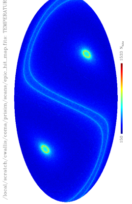
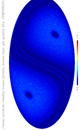
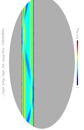
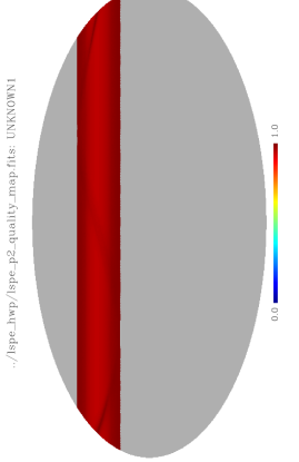
Figure 2: The hit maps (left) and polarisation coverage (right, $p_{2}$), see equation (26), of the two scan strategies used in the simulations. The plots show a full sky Mollweide projection of the sphere. Upper panels: the EPIC scan strategy (Bock et al., 2009) used to demonstrate the “extensive $\psi_{\rm t}$” range algorithm. The EPIC scan strategy is designed to mitigate systematic errors by having many crossing angles for each pixel. This projection is in Galactic coordinates. Lower panels: the LSPE scan strategy (Aiola et al., 2012) used to demonstrate the “limited $\psi_{\rm t}$” range algorithm. The LSPE gondola will perform scans of constant azimuth, changing the elevation $\sim$daily. There is, therefore, a limited range of crossing angles for each pixel. LSPE will obtain good polarisation angle coverage using a stepped HWP. This projection is in Ecliptic coordinates.

In all the simulations we use a fiducial power spectrum with a scalar-to-tensor ratio of 0.1 and lensing $B$-modes are also present.

3.1 Extensive $\psi_{\rm t}$ coverage algorithm with a satellite-like experiment

We simulate noisy TODs with systematic errors. The main source of systematics we will be considering are leakage from temperature fluctuations to polarisation fluctuations. Therefore it may be sufficient to only simulate the systematics introduced by imperfections that couple temperature to polarisation. A TOD element, $t_{j}$, is simply the temperature and polarisation response multiplied by the underlying CMB sky and then integrated,

$$t_{j} = G\int\mathbf{du}[B^{T}_{j}(\mathbf{u})T(\mathbf{u}+\Delta\mathbf{p})+B^{Q}_{j}(\mathbf{u})Q(\mathbf{u}+\Delta\mathbf{p})$$ (27)

$$\qquad\qquad\qquad\qquad\qquad\quad+B^{U}_{j}(\mathbf{u})U(\mathbf{u}+\Delta\mathbf{p})],$$

where $X(\mathbf{u})$ is the sky emission in the Stokes parameter $X$ from the direction pointed to by the unit vector $\mathbf{u}$. $B^{X}_{j}(\mathbf{u})$ is the beam response in the direction $\mathbf{u}$ for the Stokes parameter $X$ when orientated in the position $j$. $G$ is the gain of the detector and $\Delta\mathbf{p}$ is the shift in the temperature beam due to the pointing error. The position $j$ describes the orientation of the telescope by the standard Euler angles and the orientation of the HWP. In order to simulate this correctly one would need to convolve the sky over this 4 dimensional space. For a high resolution experiment this would be computationally infeasible, especially when one requires many CMB realisations. We therefore only simulate beam systematics that couple temperature to polarisation due to differential ellipticity. The second and third term of the RHS of equation (27) can be calculated simply from a polarisation map of the sky smoothed with the axisymmetric component of the beam. In our current model of the HWP in CMB experiments, the orientation of the HWP ($\psi_{\rm h}$) has no effect on the temperature response. Therefore, we only require the convolution of the beam over the 3 dimensional space $(\theta,\phi,\psi_{\rm t})$. This approximation can be formally written as,

$$t_{j} = G\int\mathbf{du}[B^{T}_{j}(\mathbf{u})T(\mathbf{u}+\Delta\mathbf{p})+A^{Q}_{j}(\mathbf{u})Q(\mathbf{u}+\Delta\mathbf{p})$$ (28)

$$\qquad\qquad\qquad\qquad\qquad\quad+A^{U}_{j}(\mathbf{u})U(\mathbf{u}+\Delta\mathbf{p})],$$

where $A^{X}_{j}(\mathbf{u})$ is the axisymmetric component of the beam response. The first term of equation (28) is calculated by a fast pixel space convolution code developed in Wallis et al. (2014) based on the algorithm described in Mitra et al. (2011). The code produces the temperature field convolved with the asymmetric beam as binned in the 3 dimensional space. In the $\theta$ and $\phi$ space we use a HEALPix pixellation (Górski et al., 2005), and in the $\psi_{t}$ space we use a linear binning. The convolution code calculates the central values of the pixels for this 3 dimensional grid. We use $N_{\rm side}{=}2048$ for the HEALPix pixelisation and the $\psi_{\rm t}$ space is separated into 80 bins. The second and third terms of equation (28) are calculated using the SYNFAST program part of the HEALPix package. Each of these codes gives us the central values of the pixelised space. We therefore, use linear interpolation to calculate the TOD element for a particular pointing.

We use this set up to simulate the TODs for one detector pair for a given scan strategy. For the temperature beam, $B^{T}$, we use an elliptical Gaussian described by

$$B^{T}(\theta,\phi)=\frac{1}{2\pi q\sigma^{2}}e^{-\frac{\theta^{2}}{2\sigma^{2}}(\cos^{2}\phi+q^{-1}\sin^{2}\phi)}.$$ (29)

Equation (29) describes the beam for detector 1. The other detector has a similar profile except it is rotated by $\pi/2$ to create a differential ellipticity between the two detectors. We use $\sigma=3$ arcmin corresponding to a FWHM of 7 arcmin and the ellipticity parameter $q=1.2$.

We include a differential gain between the detectors by simply multiplying one detector’s response by a constant gain factor. We also simulate a constant differential pointing by simply including an offset in one of the detector pointings in our simulation.

We use the EPIC scan strategy (Bock et al., 2009) in the following simulations with and without a stepped HWP, to simulate one detector pair that suffers from the systematics we consider in this paper. See Fig. 2 for the hit map of the EPIC scan strategy. We step the HWP by $\pi/8$ every 1hr. For these satellite simulations we do not include a Galactic mask. This map-making algorithm works in a very similar way to a binned map and only requires the TOD data from one pixel to create an estimate of the Stokes $Q$ and $U$ of a pixel. It will therefore work equal well regardless of the sky coverage. Here we use the entire sky to make the power spectrum analysis simple.

3.1.1 Simulation 1: No HWP included, no noise

We simulate a noise-free TOD from a detector pair that suffers from a differential gain of the two detectors of 1% and a differential pointing of 0.1 arcmin which is 1.5% of the 7 arcmin (FWHM) beam. We do not include any differential ellipticity because in this simulation we do not have a HWP. Without a HWP the spin-2 systematic created by differential ellipticity cannot be distinguished from the spin-2 polarisation signal. Therefore, the technique we present in this paper cannot remove the systematic. If an experiment needs to remove this systematic we suggest the methods presented in Ade et al. (2014) and Wallis et al. (2014). Fig. 3 shows the recovered $B$-mode power spectrum when a simple binned map is made from this TOD compared to one where the algorithm described in Section 2.1 is used. We included the terms $\tilde{S}_{0,0}$ and $\tilde{S}_{0,1}$ in equation (9) to account for the differential gain and pointing. In Fig. 3 we can clearly see that the algorithm has removed the bias on the recovered $B$-mode power spectrum as a result of the temperature to polarisation leakage.

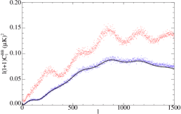
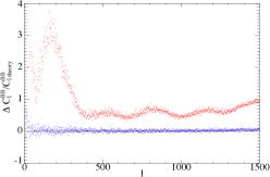
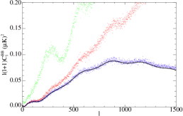
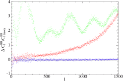
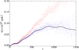
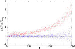
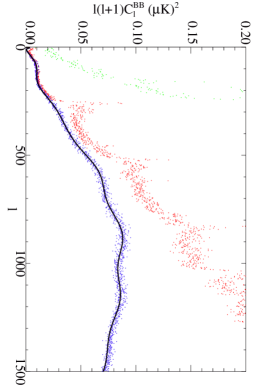
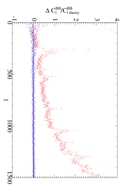
Figure 3: We show the recovered $B$-mode power spectrum for the satellite-like experiment as an example of the map-making algorithm with a extended range of $\psi_{\rm t}$ angles, see Section 2.1. The left column shows the power spectra and the right the fractional error for the simulations. The red dots show the results where a binned map is made and the blue the result when our algorithm is used, the input $B$-mode power spectra is shown in black. First row: the results from simulation 1, see Section 3.1.1, where we consider an experiment without a HWP and include differential gain and pointing systematics in the TOD. As there is no HWP we cannot apply our method to remove differential ellipticity so it is not included here. Second row: the results from simulation 2, see Section 3.1.2, where we consider an experiment with a HWP and included differential gain, pointing and ellipticity systematics in the TOD. The green dots show the recovered power spectra where a binned map is made and the TOD was created without considering a HWP to demonstrate the benefit of a HWP at mitigating systematics. Third row: the recovered power spectra for simulation 3, see Section 3.1.3. This is similar to simulation 2 but with noise included in the TOD. Fourth row: the recovered power spectra for simulation 4, see Section 3.1.4. This is similar to simulation 2 but with the CMB dipole included in the sky model and a lowed level of differetial gain, see Section 3.1.4. The green dots show the recovered power spectra where a binned map is made and the TOD was created without considering a HWP to demonstrate the benefit of a HWP at mitigating systematics.

3.1.2 Simulation 2: HWP included, no noise

We simulate a noise-free TOD from a detector pair that suffers from a differential gain of the two detectors of 1%, a differential pointing of 0.25 arcmin which is 3.5% of the 7 arcmin beam. The differential ellipticity is created using the beam described by equation (29). Figure 3 shows the recovered $B$-mode power spectrum when a simple binned map is made and a map using the algorithm described in Section 2.1. We included the terms $\tilde{S}_{0,0}$, $\tilde{S}_{0,1}$ and $\tilde{S}_{0,2}$ in equation (9) to account for the differential gain, pointing and ellipticity. Figure 3 shows that the bias created from the systematics has been removed. We also present the result when the same experiment is used but with no HWP present and when a binned map is made. This illustrates how a HWP can partially mitigate systematics. It also demonstrates that even with this mitigation, further systematic removal would be required.

3.1.3 Simulation 3: HWP included, noise included

We simulate a noisy version of the TOD used in simulation 2 described in 3.1.2. We include noise in the TOD of 1 ${\rm\mu K\sqrt{s}}$. This is optimistic for a CMB experiment. However it is chosen so that the recovered $B$-mode power is easily detected with one detector pair. The algorithm can easily deal with noise as the noise simply propagates through the matrix operation to the map in the same way as it does in a binned map-making scheme. The algorithm, however, does increase the noise on the recovered $Q$ and $U$ measurements and it also increases the covariance of the $Q$ and $U$ estimates. This increase depends on the scan strategy: the more crossing angles, the lower the increase in noise. The limiting cases of this are (1) an ideal scan strategy, where the noise increase is zero and (2) where the matrix in equation (9) is singular, in which case the effective increase in the noise is infinite. With noise simulations we have shown that the noise increase for the EPIC scan and this HWP set up is 12%. Fig. 3 shows the recovered $B$-mode power spectrum when a simple binned map is made and a map using the algorithm described in Section 2.1 and where we have removed the noise bias in each case. Again we included the terms $\tilde{S}_{0,0}$, $\tilde{S}_{0,1}$ and $\tilde{S}_{0,2}$ in equation (9) to account for the differential gain, pointing and ellipticity. Fig. 3 shows that the bias created from the systematics has been removed even in the presence of noise.

3.1.4 Simulation 4: HWP included, no noise, CMB dipole included

The CMB dipole can in principle leak to polarisation through the systematics considered in this paper and this effect can be very large. Here, we test if the map-making algorithm can remove such a level of leakage. For an experiment where the large scale modes are not filtered out at the time stream level, the leakage from the CMB dipole could be problematic. Experiments of this type do have the benefit of being able to calibrate their detectors using the CMB dipole (Planck Collaboration et al., 2015b). With this benefit in mind one would expect the differential gain for such an experiment to be lower than for ground-based experiments. To reflect this effect we lower the level of differential gain in the simulations for this section. We simulate a noise-free TOD from a detector pair that suffers from a differential gain of the two detectors of 0.2%. The other two systematics were kept the same as in simulation 2 in Section 3.1.2. Figure 3 shows the recovered $B$-mode power spectrum when a simple binned map is made and a map using the algorithm described in Section 2.1. We included the terms $\tilde{S}_{0,0}$, $\tilde{S}_{0,1}$ and $\tilde{S}_{0,2}$ in equation (9) to account for the differential gain, pointing and ellipticity. Figure 3 shows that the bias created from the systematics has been removed. We also present the result when the same experiment is used but with no HWP present and when a binned map is made. This illustrates how a HWP can partially mitigate systematics. It also demonstrates that even with this mitigation, further systematic removal would be required.

3.2 Limited $\psi_{\rm t}$ coverage algorithm with a balloon-like experiment

We test the limited $\psi_{\rm t}$ range form of our map making algorithm on a balloon like experiment. We use the LSPE scan strategy (Aiola et al., 2012) — see Fig. 2 for the hit map of the LSPE scan strategy. This is a typical balloon-like scan strategy where the gondola rotates rapidly to cover the sky. This provides good sky coverage (25% for LSPE). However, the pixels are always scanned in a similar direction. Although this can make systematic mitigation problematic, we show here that this problem can be avoided with a suitable map-making algorithm. Instead of using the range of crossing angles to accurately characterise the systematic and therefore remove it, here we assume that the systematics are slow enough functions of $\psi_{\rm t}$ that in the small range of $\psi_{\rm t}$ probed by the instrument, the combined effect can be described by a few Legendre polynomials. The maximum range of $\psi_{\rm t}$ for all the pixels in the LSPE scan strategy is $\approx$0.5 rads. Figure 1 shows that with this small range the spin-2 systematic (the fastest changing systematic we consider) can be recovered to a fraction of a percent with just the first 3 Legendre polynomials.

In the simulation we use the same beam shape as used in Wallis et al. (2014) — see Figure 1 of that paper, which has a FWHM of 1.5°. This beam is a simulation of the beam planned to be on board LPSE. We simulate TODs from a detector pair — one dectector has the same beam as the other but rotated by $\pi/2$ to provide a differential ellipticity. LSPE will achieve the required angle coverage by using a stepped HWP. We simulate this by rotating the polarisation sensitivity of the beam. We step the HWP by $\pi/8$ every hour in the simulation. We simulate the LSPE scan strategy for 15 days, each day the telescope performs scans of constant elevation. We then change the elevation daily.

Unlike in the satellite-like experiment, simulating the asymmetric beam for polarisation is feasible. Even though the asymmetry of the polarised beam will in principle create a bias that our algorithm does not remove, the resulting bias is considerably smaller than the temperature leakage. The simulation performed here is a good demonstration of this as we simulate the systematic errors such as differential pointing completely. However, we only remove the resulting temperature to polarisation leakage and we do not account for the resulting polarisation to polarisation errors.

As the amount of simulated data is much smaller for this low resolution balloon-like experiment, we do not have to make the same approximations as we do in the satellite-like experiment. We perform a pixel based integration of the beam multiplied by the CMB sky for each TOD element in the experiment. We simulate differential gain by multiplying one detector of the pair by 1.01 to create a 1% error. Differential pointing is created by changing the pointing position of the second detector’s beam by 0.05° which is 3% of the 1.5° FWHM beam. As described above the differential ellipticity is created using the simulated beam shown in figure 1 of Wallis et al. (2014). We include noise in the TOD corresponding to a noise level in the map of 0.1$~{}\mu$K per 1.5$\degree$ beam. This level of noise is optimistic for LSPE (which should achieve $\sim 7~{}\mu$K per 1.5$\degree$ beam (Bersanelli et al., 2012)). However, as an example of the algorithms ability to deal with noise, this level of noise is more than sufficient.

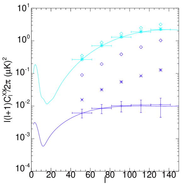
Figure 4: We plot the reconstruction of the $E$-mode and $B$-mode power spectrum for the balloon-like experiment, see Section 3.2, as an example of the map-making algorithm for a scan strategy that has a limited range of $\psi_{\rm t}$. We show the recovered power spectrum averaged over 100 realisations for maps created in three ways. The diamonds show the recovered power spectra for a binned map, the stars correspond to including the term $\tilde{S}_{0,0}$ in equation (20). Finally we show the power spectra including both $\tilde{S}_{0,0}$ and $\tilde{S}_{0,1}$ in equation (13). The resulting recovered power spectra and error bars are shown. The bias in the recovered $B$-mode has been reduced by 2 orders or magnitude to less than 5% of the error bars, which as described in Section 3.2 is for an optimistic LSPE noise.

Figure 4 shows the recovered $E$- and $B$-mode power spectrum for the balloon-like experiment. As the LSPE scan strategy only covers 25% of the sky we use a simple pseudo-$C_{\ell}$ estimator (Brown et al., 2005) to recover the polarised power spectra. We show the recovered power spectrum averaged over 100 realisations for maps created in three ways. Unlike in the extensive $\psi_{\rm t}$ range case there is little physical interpretation of the terms removed in the limited $\psi_{\rm t}$ range case. We are creating different approximations to the combined effect of the systematic $f(x)$ from equation (13). The first map-making algorithm we use assumes $f(x){=}0$. This is equivalent to a simply binned map and the recovered power spectra are shown as the diamonds in figure 4. The bias from the binned map is obvious. We can improve this by including the term $\tilde{S}_{0,0}$ in equation (20). This makes the approximation $f(x){=}{\rm const}$ and reduces the bias by an order of magnitude, as shown in Fig. 4 as the stars. Finally we improve this further by assuming that $f(x)$ is a linear function. This is done by including both $\tilde{S}_{0,0}$ and $\tilde{S}_{0,1}$ in equation (13). The resulting recovered power spectra and error bars are shown in Fig. 4. The bias in the recovered $B$-mode has been reduced by 2 orders or magnitude to less than 5% of the error bars, which as described above are error bars for an optimistic LSPE noise level.

Figure 4 clearly demonstrates that our technique can remove the bias as a result of temperature to polarisation leakage. However, this comes at the cost of a noise penalty in the map. Including the $\tilde{S}_{0,0}$ only and adopting $f(x){=}{\rm const}$ incurs a 5% increase in the noise power with respect to the binned map. The analysis where $f(x)$ is modelled as a linear function and both $\tilde{S}_{0,0}$ and $\tilde{S}_{0,1}$ terms are included in equation (13) creates an increase in the noise power of 12% with respect to a binned map.

4 Identifying Systematics

The extensive $\psi_{\rm t}$ range map-making algorithm relies on being able to remove systematics which have different Fourier modes in $(\psi_{\rm t},~{}\psi_{\rm r})$ space to that of the polarisation signal. As discussed in section 2, the map-making algorithm requires us to know that the systematics are present in the TOD so that we can choose to include the correct Fourier modes in equation (9) and create maps that are clean of those systematics. We stress that we do not need to know the exact nature of the systematic. For example, if the experiment is suffering from differential pointing of the detector pair, at no point do we need to know by how much or in what orientation the beams are misaligned. Moreover, we do not require a temperature map to remove the signal. This is an improvement over the method used in Ade et al. (2014). We only need to know that the experiment is suffering from differential pointing and therefore we know to include the $\tilde{S}_{0,1}$ term in the analysis. One down side of using this method to clean systematics is the increase in statistical noise. Every term included in the analysis increases the statistical noise of the recovered polarisation maps, and also the cross correlation of Stokes $Q$ and $U$. The level of the increase is dependent upon the scan strategy — the more extensive $(\psi_{\rm t},\psi_{\rm r})$ coverage the experiment has, the smaller the increase of noise. We demonstrated this with simulations of the EPIC scan strategy (see Section 3). The increase in the noise power spectrum, going from a binned map to our map-making algorithm accounting for all three systematics, was 12%. This would be lower if not all systematics were considered. With this increase of noise in mind it would be undesirable to include terms needlessly, but we also do not want to create a bias by neglecting a term if the systematic is present.

We now turn our attention to a practical process to determine whether a potential systematic should be removed. We start by making a map of the systematic. This is done in the same way that the $Q$ and $U$ maps are made. The inversion of equation (9) will give us an estimate for the $\tilde{S}_{n,m}$ terms we included. By taking the real and imaginary parts of this we can make a map of our systematics. Figure 5 shows maps of the systematics recovered from simulation 3 described in Section 3.1.3. We also show the predictions for each systematic based on prior knowledge, and finally, the difference between the prediction and recovered systematic maps. This figure demonstrates how we can accurately recover the systematics without any prior knowledge of the instrumental imperfections or of the underlying temperature field.

	Recovered in map-making	Predicted using simulation inputs	Difference
(a)
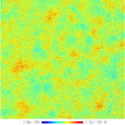
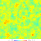
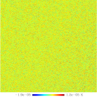
(b)
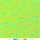
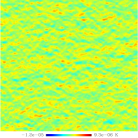
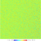
(c)
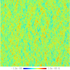
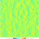
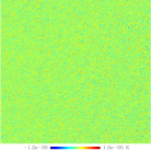
(d)
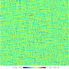
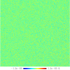
(e)

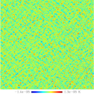
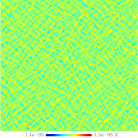
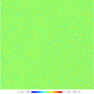
Figure 5: Each row shows the systematic from the noisy TOD in simulation 3 described in Section 3.1.3. Each section of the sky is a gnomonic projection of a 12.5$\degree$ square patch of sky. We plot the map extracted using the systematic map making method described in Section 2 on the left. The middle column displays a prediction for the systematic based on prior knowledge. The right column shows the difference which in each case is compatible with noise. Row (a) shows the results for differential gain ($\tilde{S}_{0,0}$), rows (b) and (c), differential pointing ($\Re[\tilde{S}_{0,1}]$ and $\Im[\tilde{S}_{0,1}]$) and rows (d) and (e) show the differential ellipticity systematic ($\Re[\tilde{S}_{0,2}]$ and $\Im[\tilde{S}_{0,2}]$).

The top row of Figure 5 shows the map of differential gain. As this is a spin-0 term there is only one non-trivial map to show. The prediction is created by convolving the temperature field with the beam and multiplying it by the size of the differential gain. The difference is consistent with noise as a result of the noise in the TOD. Rows 2 and 3 show maps of differential pointing. Being spin-1, row 2 shows the error if the instrument was oriented with $\psi_{\rm t}{=}0$ and row 3 shows the error if the telescope was orientated with $\psi_{\rm t}{=}\pi/2$. The systematic error on a TOD sample is simply a rotation of this spin-1 vector. The prediction is created by using the first differential of the temperature map and multiplying the results by half the angular size of the differential pointing. Rows 4 and 5 are maps of the differential ellipticity. As the differential ellipticity is a spin-2 systematic we are only able to make the distinction between the systematic and the polarisation using the HWP. The fields depicted in rows 4 and 5 are similar to the Stokes $Q$ and $U$ fields respectively. The prediction was created by using the underlying temperature field and the beam shape used in the simulation. It was shown in Wallis et al. (2014) that the spin-2 systematic would have the form,

$$\Delta a^{E}_{\ell m} = \sqrt{\frac{4\pi}{2\ell+1}}\Re(b^{\rm diff}_{\ell 2})a^{T}_{\ell m},$$ (30)

$$\Delta a^{B}_{\ell m} = i\sqrt{\frac{4\pi}{2\ell+1}}\Im(b^{\rm diff}_{\ell 2})a^{T}_{\ell m},$$ (31)

where $\Delta a^{E}_{\ell m}$ and $\Delta a^{B}_{\ell m}$ are the $E$ and $B$-mode of the systematic, $a^{T}_{\ell m}$ is the spherical harmonic decomposition of the temperature field and $b^{\rm diff}_{\ell 2}$ is the second azimuthal mode of the spherical harmonic decomposition of the difference of the two temperature beams in the detector pair.

Figure 5 shows that the map-making algorithm can correctly recover maps of the systematic errors. However, the maps are noisy. One can imagine a situation where the noise level is too large to see the systematic but there is a non-negligible effect on the recovered $B$-mode power spectrum. This will be especially true when many detectors are considered as the maps would have to be made for each detector pair. However, since each of the systematics couple to the temperature field, the recovered maps of the systematics will correlate with the temperature field.

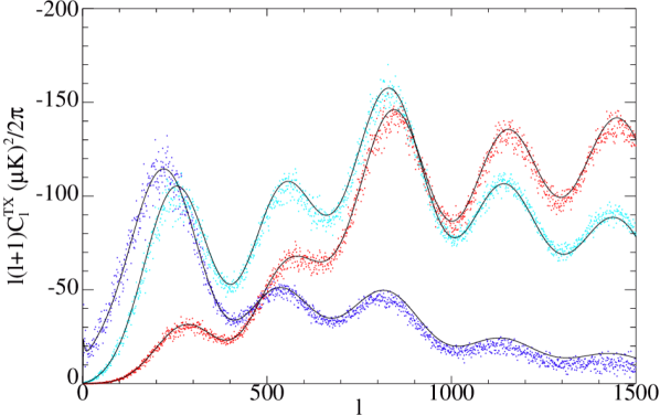
Figure 6: We plot the cross-correlation of the systematic maps (see Figure 5) with the temperature map created using the TOD in simulation 3 in Section 3. The cross-power spectrum is a good method to find systematics that may be below the noise level in the systematic maps. The differential gain systematic error map cross correlated with the temperature map is plotted in dark blue dots. The light blue dots show the differential pointing maps cross correlated with the temperature map. The differential ellipticity map cross correlated with the temperature map is shown as the red dots. Over plotted are $N_{0}C^{T}_{\ell}$, $N_{1}\ell C^{T}_{\ell}$, $N_{2}\ell^{2}C^{T}_{\ell}$, where $N_{i}$ are normalisation factors. This demonstrates that the systematics are simply the temperature field convolved with the beam, or derivatives thereof.

In Fig. 6 we plot the cross-power spectrum between systematic maps and the temperature map created using the TOD used in the simulation, where we have also deconvolved for the beam. We have over plotted $N_{0}C^{T}_{\ell}$, $N_{1}\ell C^{T}_{\ell}$, $N_{2}\ell^{2}C^{T}_{\ell}$, where $N_{i}$ are normalisation factors calculated by minimising the absolute residuals between the model and the cross-power spectrum. This demonstrates the known result that the systematics are simply the temperature field, or some derivative of the temperature field. Even in a noisy systematic map the cross-power spectrum will provide a valuable insight to the size of a systematic effect. We recover a non-zero correlation because the systematics are present in the TOD. If this were not the case and the TOD was clean then we would find a cross-power spectrum consistent with zero. This provides us with a recipe to test for the presence or absence of systematic effects: if, in an experiment, this cross-power spectrum is shown to be consistent with zero then the maps can be (re-)made not accounting for this systematic. The resulting increase of noise in the map, with respect to a binned map, would thus be kept to a minimum.

5 Discussion

We have developed two map-making algorithms to remove common systematics that couple temperature to polarisation in differencing CMB polarisation experiments. The result of the map-making algorithms is the polarisation sky smoothed with the axisymmetric part of the beam used. The systematics we consider are differential gain, pointing and ellipticity of two detectors in a detector pair, all of which were shown to be an issue in the BICEP2 experiment (Ade et al., 2014). The main issue with these systematics is the leakage from temperature to polarisation that they create. Shimon et al. (2008) showed that the coupling from temperature to polarisation of these systematics have spin-0,1 and 2 properties respectively. We used this understanding to develop the algorithm used here.

The first algorithm, described in Section 2.1, removes the systematics by separating the Fourier modes of the systematics and the Fourier mode of the polarisation, using equation (9). The technique requires a suitable scan strategy. The angle coverage of the orientation of the telescope, $\psi_{\rm t}$, must be extensive to allow for the different Fourier modes to be distinguished. We have shown through simulations in Section 3.1 that the EPIC (Bock et al., 2009) scan strategy provides the required amount of angle coverage.

In Section 3.1 we demonstrated the effectiveness of the algorithm through three simulations. Simulation 1 showed the ability of the technique to remove differential gain and pointing when a HWP is not used. Without a HWP the spin-2 systematic and the polarisation signal are degenerate and, therefore, cannot be separated using this technique. In this case we suggest using the methods proposed in Wallis et al. (2014) and Ade et al. (2014). The technique however, can remove differential gain and pointing as they have a different spin to the polarisation signal. In Section 3.1.2 and 3.1.3 we presented simulations including a HWP. In these simulations we showed that the technique can simultaneously remove differential gain, pointing and ellipticity. The CMB dipole can contribute to the leakage from temperature to polarisation. We demonstrated in Section 3.1.4 that the map-making algorithm can deal with this level of leakage.

One draw back to this technique is an increase in the statistical noise in the resultant (cleaned) $Q$ and $U$ maps. The level of the noise increase is dependent on the scan strategy — the more even the $\psi_{\rm t}$ angle coverage, the lower the increase in noise. An ideal experiment would suffer no increase in noise. At the other extreme where the coverage is not large enough, the matrix in equation (9) becomes singular and the effective increase in noise is infinite. Through simulations we have shown that the increase in noise power for simulation 3 is 12% when compared to a binned map.

The second algorithm, described in Section 2.2, removes the temperature to polarisation leakage by creating a model for total leakage as a function of the orientation of the telescope. The combined effect of the systematic is modelled as a smooth function of the orientation angle. With this assumption we can then describe the combined systematic $f(x)$ by a few Legendre polynomials. Figure 1 shows that a spin-2 systematic can accurately be reconstructed by the first three Legendre polynomials, with a $\psi_{\rm t}$ range of 0.5 rads. This $\psi_{\rm t}$ range was chosen to be representative of the LSPE scan strategy (Aiola et al., 2012), where the maximum $\psi_{\rm t}$ range is $\approx$0.5 rads. In Section 3.2, we demonstrated that the algorithm can remove the temperature to polarisation leakage from differential gain, pointing and ellipticity in a simulation where the LSPE scan strategy was used with a stepped HWP. As with the extensive $\psi_{\rm t}$ range technique there is an increase in the statistical noise of the polarisation maps when using this technique. Through simulations we showed that the increase of noise using the LSPE scan strategy was 12%.

In Section 4 we have presented a method to identify if systematics are present in a TOD. The extensive $\psi_{\rm t}$ range algorithm separates the systematics into Fourier modes and generates an estimate of the polarisation free of these systematics. It also at the same time creates an estimate of the systematic. We showed in Fig. 5 the maps of the systematics recovered from simulation 3 (see Section 3.1.3). These maps can be used to identify if a systematic is present. However, the noise in the TOD and the relative size of the systematic effect could render the reconstructed maps too noisy to see the systematic easily. To increase the signal-to-noise, we suggest calculating the cross-power spectrum of these systematic maps with the temperature map. As the systematics we are considering are due to temperature to polarisation leakage then, if the systematic is present, we expect to see a non-zero cross-correlation. We showed the cross-power spectrum between the systematic maps and the temperature map created using the TOD in Fig. 6. This technique can be used to identify if systematics are present. This is crucial to test the validity of an experiment’s polarisation maps, but could also be used to identify whether a systematic must be removed using this technique. Accounting only for those systematics that are actually present in the TOD would minimise the increase in noise associated with the correction algorithms developed in this work.

References

- Ade et al. (2014) Ade P. A. R., et al., 2014, Physical Review Letters, 112, 241101
- Aiola et al. (2012) Aiola S., et al., 2012, in Society of Photo-Optical Instrumentation Engineers (SPIE) Conference Series. , doi:10.1117/12.926095
- BICEP2 Collaboration et al. (2015) BICEP2 Collaboration et al., 2015, preprint, (arXiv:1502.00608)
- BICEP2/Keck and Planck Collaborations et al. (2015) BICEP2/Keck and Planck Collaborations et al., 2015, Physical Review Letters, 114, 101301
- Baxter et al. (2014) Baxter E. J., et al., 2014, preprint, (arXiv:1412.7521)
- Bersanelli et al. (2012) Bersanelli M., et al., 2012, in Society of Photo-Optical Instrumentation Engineers (SPIE) Conference Series. p. 7 (arXiv:1208.0164), doi:10.1117/12.925688
- Bock et al. (2009) Bock J., et al., 2009, preprint, (arXiv:0906.1188)
- Brown et al. (2005) Brown M. L., Castro P. G., Taylor A. N., 2005, MNRAS, 360, 1262
- Brown et al. (2009a) Brown M. L., Challinor A., North C. E., Johnson B. R., O’Dea D., Sutton D., 2009a, MNRAS, 397, 634
- Brown et al. (2009b) Brown M. L., et al., 2009b, ApJ, 705, 978
- Crites et al. (2014) Crites A. T., et al., 2014, preprint, (arXiv:1411.1042)
- Das et al. (2014) Das S., et al., 2014, Journal of Cosmology and Astroparticle Physics, 4, 14
- Górski et al. (2005) Górski K. M., Hivon E., Banday A. J., Wandelt B. D., Hansen F. K., Reinecke M., Bartelmann M., 2005, ApJ, 622, 759
- Hanson et al. (2013) Hanson D., et al., 2013, Physical Review Letters, 111, 141301
- Mitra et al. (2011) Mitra S., Rocha G., Górski K. M., Huffenberger K. M., Eriksen H. K., Ashdown M. A. J., Lawrence C. R., 2011, APJS, 193, 5
- Planck Collaboration et al. (2014a) Planck Collaboration et al., 2014a, preprint, (arXiv:1409.5738)
- Planck Collaboration et al. (2014b) Planck Collaboration et al., 2014b, A&A, 571, A1
- Planck Collaboration et al. (2014c) Planck Collaboration et al., 2014c, A&A, 571, A17
- Planck Collaboration et al. (2014d) Planck Collaboration et al., 2014d, A&A, 571, A22
- Planck Collaboration et al. (2015a) Planck Collaboration et al., 2015a, preprint, (arXiv:1502.01582)
- Planck Collaboration et al. (2015b) Planck Collaboration et al., 2015b, preprint, (arXiv:1502.01587)
- Shimon et al. (2008) Shimon M., Keating B., Ponthieu N., Hivon E., 2008, Phys. Rev. D, 77, 083003
- Story et al. (2013) Story K. T., et al., 2013, ApJ, 779, 86
- The Polarbear Collaboration: P. A. R. Ade et al. (2014) The Polarbear Collaboration: P. A. R. Ade et al., 2014, ApJ, 794, 171
- Wallis et al. (2014) Wallis C. G. R., Brown M. L., Battye R. A., Pisano G., Lamagna L., 2014, MNRAS, 442, 1963
- Wu et al. (2007) Wu J. H. P., et al., 2007, ApJ, 665, 55