Stochastic Texture Difference for Scale-Dependent Data Analysis

Abstract

This article introduces the Stochastic Texture Difference method for analyzing data at prescribed spatial and value scales. This method relies on constrained random walks around each pixel, describing how nearby image values typically evolve on each side of this pixel. Textures are represented as probability distributions of such random walks, so a texture difference operator is statistically defined as a distance between these distributions in a suitable reproducing kernel Hilbert space. The method is thus not limited to scalar pixel values: any data type for which a kernel is available may be considered, from color triplets and multispectral vector data to strings, graphs, and more. By adjusting the size of the neighborhoods that are compared, the method is implicitly scale-dependent. It is also able to focus on either small changes or large gradients. We demonstrate how it can be used to infer spatial and data value characteristic scales in measured signals and natural images.

I Introduction

I-A What this work is about

In this paper, we present a local algorithm, a low-level and scale-dependent data analysis that is able to identify characteristic scales in data sets, for example (but not limited to) images. The main idea is to statistically characterize how data values evolve when exploring each side of a given pixel, then compare the statistical properties of each side. We exploit random walks on images but in a different setting than [1]. Our method resembles the graph walks in [2], except that we additionally introduce a statistical comparison operator, that our method is adapted to images, directional, accounts for neighborhood information and is intrinsically scale-dependent. Indeed, exploring the neighborhood of each pixel implies setting two scales: the spatial extent of that exploration, and the sensitivity to pixel value differences along each explored path. Once these are set, we quantify the difference between each side, and repeat the operation in other orientations around a pixel. This gives, for each pixel and each prescribed set of (spatial, data) scales, a measure of how that pixel is a transition between distinct statistical properties on each of its sides. Depending on how these scales are set, we may for example get a new kind of low-level boundary detector, sensitive to either small data changes or large gradients, and at different resolutions. The method can be used to infer characteristic scales in natural data, these at which the boundaries capture most of the information. The method is not restricted to images, it is readily extendable to voxels or other spatially extended data (e.g. irregular meshes). It is not restricted either to scalar (e.g. gray) valued pixels: any data type for which a reproducing kernel is available can be used (e.g. vector, strings, graphs). We present in particular the case for color triplets in Section VI.

I-B What this work is not about

Our goal is to provide a local algorithm, that works at pixel level, and not to perform global image segmentation. The best algorithms for segmentation account for texture information [3], exploit eigen-decompositions for identifying similar regions [4], or improve their results with edge completion [5]. These high-level operations are very efficient at finding transitions between general zones in the image [6], but we want a local quantifier that can be used to infer characteristic scales within acquired data, which is a different problem from image segmentation. It may be the case that our methodology becomes useful in a segmentation context, but this topic is out of the scope of the present paper.

Similarly, our goal is not to perform high-level texture classification [7], but to formulate a new way to represent textures and their differences (Section III). As a quantifier for texture differences, our method might provide future works with a new way to compare an unknown sample with a reference database. However, it remains to be seen how efficient that would be compared to well-established alternatives. In particular, we do not decompose data on a basis of functions, such as wavelets [8], curvelets [9], bandelets [10] and other variants [11]. Neither do we adapt the decomposition basis using a dictionary [12] or define elementary textons [13] for description and classification purposes. We compare distribution of probabilities, which we identify with the textures. It may be that our method ultimately helps in defining new optimal decomposition of images on some basis of elementary textures, but that is another issue, which falls out of the scope of this article.

I-C Comparison with related approaches

Multi-scale analysis can either be performed by exploiting relations and patterns across scales, or by defining features per scale, and then investigating how these evolve as the scale varies. The first category includes all wavelet-based methods mentioned above, as well as more advanced techniques like multifractal analysis [14, 15]. By definition, methods in this first family do not allow finding characteristic scales, they exploit relations between scales, for example to build texture descriptors. The second category, a scale-dependent analysis which is then repeated at multiple scales, is prominently represented in the field of image processing by space-scale decompositions [16]. This way, edges are found at different levels of details [17], hopefully allowing the user to remove all extraneous changes and focus on important object boundaries [18]. Any scale dependent analysis might be used in this second family, and in particular pixel connectivity, which is sometimes used to obtain multiscale descriptions, see [19] for a review. Our method falls in the second category, but with a completely new feature involving sets of random paths. It allows to specify both the spatial scale and the data scale for the analysis, and to look for optima in this two-dimentional parameter space which are presumably characteristic of the data, see Section V.

We then use statistics to quantify how data values evolve in a pixel neighborhood at these prescribed spatial and data scales. [20] also uses statistics to compare data distributions at multiple scales, but with a different framework and for classification purposes. We use random walks in order to explore the neighborhoods. Although we use a Markov Random Field (MRF) approach in order to fix the random walk transition probabilities, our approach is fundamentally different from the typical use of MRF in image processing (see [21] for a review). We use the MRF solely as a intermediate step to calibrate the random walks with a spatial scale, and not as a model for pixel values, or for segmentation [1, 22]. Anisotropic diffusion methods, from the Perona-Malik model [23] to space-scale extensions with partial differential equations [24], might seem related to this random walk approach. Indeed, gaussian filtering could be seen as integrating pixel values along random paths in the neighborhoods we use. However, we do not integrate along random paths, but we rather exploit how pixel values evolve along these paths in order to define a statistical distribution of these variations in the neighborhood, which we then identify with texture information (Section III-B). Our method can thus be seen as complementary to diffusion. A notable multiscale extension of anisotropic diffusion to vector data can be found in [25], and it would be interesting to compare how introducing a reproducing kernel in their setup complements our own technique.

Our method is applicable to non-scalar data, including non-vector data, by means of reproducing kernels. Yet, we do not use kernel methods as in machine learning of texture features [26, 7], but as an indirect way to quantify discrepancies between probability distributions, building on recent findings in statistics [27, 28]. Consequently, for the particular case of kernels on color spaces which we demonstrate in Section VI, our method is fundamentally different from current approaches in the domain [29]. Our hope is that this ability to work with non-scalar data will make our method a prominent tool for the analysis of multispectral and other kind of images.

The stochastic texture discrepancy (STD) which we present can also be seen as a kind of “texture gradient” (see Section V-C). Unlike related work, which use wavelet transforms [30], morphological operations [31], or combinations of both [32] to define texture gradients, the STD is a norm in a suitable reproducing kernel Hilbert space. Consequently, we expect that it could be also incorporated in classic gradient-based edge-detection algorithms [33], or any other setup in which a proper norm is required.

Section II presents the theory, starting with how texture is encoded and Section III how texture information is compared on each side of a pixel. Section IV gives a first application of the method, how it can detect texture boundaries accouting for scale information. Section V builds on this and presents a fully automated method for detecting characteristic scales in acquired data (including, as in this paper, images). Section VI demonstrates that our method deals equally well with non-scalar data, including, in that application case, color triplets. Color texture difference is shown to better detect boundaries and highlight small details than alternatives.

II Encoding texture information

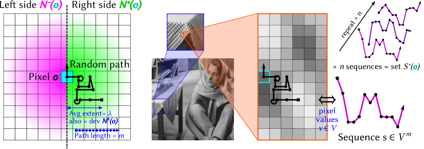
Figure 1: General method for generating stochastic texture descriptions. The case for a left/right split is presented, but other orientations with any angle are processed in exactly the same way. Notations and a step by step description are given in the main text.

In the following, bold mathematical symbols denote pixels, plain symbols are values associated to these pixels. Capital mathematical symbols (resp. bold, plain) represent sets (of resp. pixels, values). Mathematical spaces are calligraphied.

II-A Overview

Consider a pixel $\boldsymbol{o}$. An orthonormal basis $\left(\vec{x},\vec{y}\right)$ in the image plane being fixed (for instance the one aligned with the boundaries of the image), we consider the affine basis $\left(\boldsymbol{o},\vec{x},\vec{y}\right)$ with the origin at that pixel center. We want to compare how the texture on the half-plane $\{x>0\}$ is statistically different from the texture on the other side $\{x<0\}$ (Fig. 1). A length scale is needed to characterize the extent of the texture comparison within each half-plane. Let $\lambda$ be this spatial length scale. Noting $\boldsymbol{N}^{\pm}(\boldsymbol{o})$ neighborhoods of pixels within the two half-planes, consider the probability densities defined on $\boldsymbol{N}^{\pm}(\boldsymbol{o})$ by $p^{\pm}(x,y)=C\cdot\exp\left(-\frac{x^{2}+y^{2}}{2\lambda^{2}}\right)$ for $\pm x\geq 0$ and $0$ otherwise, where $C$ is a normalizing constant. The texture characterization we propose amounts to:

A: monitoring pixel values taken along $n$ independent random paths in each of these neighborhoods $\boldsymbol{N}^{\pm}(\boldsymbol{o})$;

B: in a way that the probability to visit a pixel $\boldsymbol{a}\in\boldsymbol{N}^{\pm}(\boldsymbol{o})$ is given by $p^{\pm}(\boldsymbol{a})=\iint_{x,y\in\boldsymbol{a}}p^{\pm}(x,y)\mbox{d}x\mbox{d}y$;

C: and that the average spatial extent of a random path is $\lambda$.

As a result of this process, two sets $S^{\pm}(\boldsymbol{o})$ are obtained for each pixel $\boldsymbol{o}$ along each pair of opposite directions. These sets each contain $n$ random sequences of pixel values $\left(v\left(\boldsymbol{a}_{i}\right)\right)_{i=1\ldots m}$, with $v(\boldsymbol{a})$ the image information (gray scale, RGB, etc.) at pixel $\boldsymbol{a}$. A set of paths thus contains the statistical description of a texture on the corresponding side of a pixel $\boldsymbol{o}$, at a prescribed characteristic spatial scale of $\lambda$.

Each of the above points is detailed separately in the following subsections.

II-B Generating random paths

Each pixel location around $\boldsymbol{o}$ is considered to be a distinct state of a Markov chain. Transitions are allowed to the 4 neighborhood pixels, together with self-transitions. A random pixel in $\boldsymbol{a}_{1}\in\boldsymbol{N}^{\pm}(\boldsymbol{o})$ is chosen as the starting point, with a probability given by the limit distribution $p^{\pm}\left(\boldsymbol{a}_{1}\right)$.

The Markov chain is then run for $m$ steps for generating the pixel sequence $\left(\boldsymbol{a}_{i}\right)_{i=1\ldots m}$. The values of these pixels are then taken along this path, so that $s=\left(s_{i}=v\left(\boldsymbol{a}_{i}\right)\right)_{i=1\ldots m}\in S^{\pm}(\boldsymbol{o})$ is a length $m$ excerpt of the texture in $\boldsymbol{N}^{\pm}(\boldsymbol{o})$. The process is repeated $n$ times to get the full set $S^{\pm}(\boldsymbol{o})$, in each direction, which is assumed to encode the full texture information provided $n$ is large enough (Fig. 1).

II-C Building the Markov chain

For each pixel $\boldsymbol{a}$, hence each state of the Markov chain, we first compute $p^{\pm}(\boldsymbol{a})$. This is the probability of reaching this state in the limit distribution of the Markov chain. We now need to define a set of transitions that leads to this limit distribution.

Let $p^{\pm}(\boldsymbol{a}\rightarrow\boldsymbol{b})$ be the transition probability from state/pixel $\boldsymbol{a}$ to state/pixel $\boldsymbol{b}$. There are at most 5 non-null such probability transitions, from $\boldsymbol{a}$ to its neighborhood pixels $\boldsymbol{b}_{1\ldots 4}$ and to itself $\boldsymbol{b}_{5}=\boldsymbol{a}$. The Markov chain is consistent with the limit distribution when:

$$p^{\pm}(\boldsymbol{a})=\sum_{i=1}^{5}p^{\pm}(\boldsymbol{b}_{i})p^{\pm}(\boldsymbol{b}_{i}\rightarrow\boldsymbol{a})$$ (1)

while respecting the constraint

$$\sum_{i=1}^{5}p^{\pm}(\boldsymbol{a}\rightarrow\boldsymbol{b}_{i})=1$$ (2)

The unknowns in this problem are the transition probabilities for every pair $\boldsymbol{a},\boldsymbol{b}$. We start by assigning initial transition probabilities $p_{ini}^{\pm}\left(\boldsymbol{a}\rightarrow\boldsymbol{b}_{i}\right)=p^{\pm}(\boldsymbol{b}_{i})/\sum_{i=1}^{5}p^{\pm}(\boldsymbol{b}_{i})$. This, of course, does not provide the correct transition probabilities, just a starting point. We then run an iterative Levenberg-Marquardt optimisation scheme in order to solve Eq.1 and Eq.2.

II-D Ensuring sequences are consistent with the spatial scale

For each sequence length $m$, we note the average extent $e(x)$ in $x$ for generated sequences of this size: $e(x)=\left\langle\max_{i\leq m}\left(\bar{x}\left(\boldsymbol{a}_{i}\right)\right)-\min_{i\leq m}\left(\bar{x}\left(\boldsymbol{a}_{i}\right)\right)\right\rangle$, with $\bar{x}\left(\boldsymbol{a}\right)$ denoting the $x$ coordinate of the center of pixel $\boldsymbol{a}$. Averaging $e(x)$ is done numerically over a large number of samples. We then select the value of $m$ that gives a sequence of spatial extent $e(x)=\lambda$ on average. The typical error on $\lambda$ is less than $0.01$ pixel for the neighborhoods we use.

Building the Markov chain and defining $m$ needs to be done only once for each neighborhood size $\lambda$ and for each considered orientation of the neighborhoods $\boldsymbol{N}^{\pm}(\boldsymbol{o})$. Distinct orientations lead to distinct $p^{\pm}(\boldsymbol{a})=\iint_{x,y\in\boldsymbol{a}}p^{\pm}(x,y)\mbox{d}x\mbox{d}y$ for every pixel $\boldsymbol{a}$ around $\boldsymbol{o}$. We limit ourselves in this paper to straight and diagonal orientations, so the densities $p^{\pm}(\boldsymbol{a})$ present a convenient symmetry in each of these two cases, but any angle is possible. Once these are precomputed, the same (straight, diagonal) Markov chains can be applied to each pixel $\boldsymbol{o}$ in the image (boundary conditions are dealt with in Section III-D).

III Comparing textures

The procedure described in the previous section is applied to each pixel on an image, leading to 4 pairs of sets $S^{\pm}(\boldsymbol{o})$ for each pixel $\boldsymbol{o}$, corresponding to both straight and diagonal directions. Each set comprises $n$ sequences $s=\left(s_{i}=v\left(\boldsymbol{a}_{i}\right)\right)_{i=1\ldots m}$ of length $m$, with $m$ chosen so that sequences extend spatially to a characteristic scale $\lambda$ in the corresponding direction on average. This section details how to quantify the difference $d\left(S^{-},S^{+}\right)$ between two sets $S^{\pm}(\boldsymbol{o})$, hence between textures on opposite sides of a pixel.

III-A Comparing two sequences of pixel values

Let $s=\left(s_{i}=v\left(\boldsymbol{a}_{i}\right)\right)_{i=1\ldots m}$ be a sequence as defined above. Let $\mathcal{V}$ be the space taken by pixel values $v(\boldsymbol{a})\in\mathcal{V}$, so that $s\in\mathcal{V}^{m}$. Consider a kernel $k:\,\mathcal{V}^{m}\times\mathcal{V}^{m}\rightarrow\mathbb{R}$, such that:

– $k\left(s,\cdot\right)$ is a function, in the Hilbert space $\mathcal{H}$ of functions from $\mathcal{V}^{m}$ to $\mathbb{R}$.

– For any function $f\in\mathcal{H}$ and for all $s\in\mathcal{V}^{m}$, the reproducing property holds: $\left\langle f,k(s,\cdot)\right\rangle_{\mathcal{H}}=f(s)$ with $\left\langle\cdot,\cdot\right\rangle_{\mathcal{H}}$ the inner product in $\mathcal{H}$.

– $\mathrm{Span}\left\{k(s,\cdot)\right\}_{s\in\mathcal{V}^{m}}$ is dense in $\mathcal{H}$

As a special case, the kernel value $k\left(s^{-},s^{+}\right)=\left\langle k\left(s^{-},\cdot\right),k\left(s^{+},\cdot\right)\right\rangle_{\mathcal{H}}$ gives the similarity between $s^{-}$ and $s^{+}$. As is customary, we normalize $k$ such that $k\left(s,s\right)=1$ and $k\left(s,t\neq s\right)<1$ for all $s,t\in\mathcal{V}^{m}$.

This classic reproducing kernel Hilbert space (RKHS) representation lets us consider any pixel value: scalar (e.g. gray scale, reflectance), vector (e.g. RGB, hyperspectral components), or in fact any kind of data for which a kernel is available (e.g. graph, strings). Indeed, once a kernel is available for an element $s_{i}\in\mathcal{V}$, it is always possible to use the product kernel for the sequence $s\in\mathcal{V}^{m}$, hence to compute the similarity between two sequences. The method we present is thus generic, and applicable to wide range of “images”, broadly defined as spatially extended data. In particular, one way to handle color textures is presented in Section VI. Similarly, definitions in Section II are easily extended to more than 2 spatial dimensions if needed (e.g. Markov chains transitions to the 6 voxel neighbors in 3 dimensions), or even to non-regular meshes (by computing $p^{\pm}(\boldsymbol{a})$ for each mesh cell and transitions as above), or graphs (provided a meaninful $p^{\pm}(\boldsymbol{a})$ can be provided for each node $\boldsymbol{a}$).

III-B Quantifying texture differences

The random sequences defined above can be seen as samples of an underlying probability distribution over $\mathcal{V}^{m}$, which we identify with the texture information. It is possible that visually distinct patterns lead to the same distribution over $\mathcal{V}^{m}$, as we offer no uniqueness proof, and especially with $n<\infty$. However, the same visual ambiguity exists for other and widely used texture representation methods, for example when retaining only a small number of components in a suitable decomposition basis ([9, 10, 4]). We make no claim on the superiority of our method in this respect, but it certainly offers a very different characterization of textures, complementary to other approaches.

Let us thus identify a texture as a probability distribution $P(s)$ over $\mathcal{V}^{m}$. In this view, the sets $S^{\pm}(\boldsymbol{o})$ are collections of observed samples for the textures in the neighborhoods $\boldsymbol{N}^{\pm}(\boldsymbol{o})$. Quantifying the texture difference $d\left(S^{-},S^{+}\right)$ amounts to performing a two-sample test for similar distributions, with similarity defined by a metric on probability distributions. Using the above RKHS representation, we exploit recent litterature [27, 28] to propose a consistent estimator for $d\left(S^{-},S^{+}\right)$ that works reliably even for small number of samples $n$, irrespectively of the dimension of $\mathcal{V}$ and $\mathcal{V}^{m}$:

– For a distribution $P$, the average map $\mu_{P}\in\mathcal{H}$ is given by $\mu_{P}=E_{P}\left[k(s,\cdot)\right]$.

– An estimator $\hat{\mu}_{S}$ is easily obtained from the sample set $S$, in the form $\hat{\mu}_{S}=\frac{1}{n}\sum_{j=1}^{n}k\left(s^{j},\cdot\right)$, where $s^{j}$ denotes the $j$-th member of the set $S$.

– Let $P$ and $Q$ be two distributions over $\mathcal{V}^{m}$. If the kernel is characteristic, then $P=Q$ if and only if $\left\|\mu_{P}-\mu_{Q}\right\|_{\mathcal{H}}=0$. If $P\neq Q$, the norm directly quantifies the discrepancy between these distributions.

Thus, the texture difference $d\left(S^{-},S^{+}\right)$ can be estimated with:

$$d^{2}\left(S^{-},S^{+}\right)=\left\|\hat{\mu}_{S^{+}}-\hat{\mu}_{S^{-}}\right\|_{\mathcal{H}}^{2}$$ (3)

$$=\left\langle\hat{\mu}_{S^{+}}-\hat{\mu}_{S^{-}},\hat{\mu}_{S^{+}}-\hat{\mu}_{S^{-}}\right\rangle_{\mathcal{H}}$$

$$=\frac{1}{n^{2}}\sum_{j=1}^{n}\sum_{k=1}^{n}\left(k\left(s_{+}^{j},s_{+}^{k}\right)+k\left(s_{-}^{j},s_{-}^{k}\right)-2k\left(s_{+}^{j},s_{-}^{k}\right)\right)$$

Thanks to being a consistent estimator [28] for a norm in a suitable space, the operation we propose behaves very much like a pixel-based gradient norm, but on textures differences instead of pixel values, realizing of form of “texture gradient” (See Section V-C).

We define an overall Stochastic Texture Discrepancy $\textrm{STD}(\boldsymbol{o})$ for each pixel $\boldsymbol{o}$ by considering the norm in the product space $\bigotimes_{\theta}\mathcal{H}_{\theta}$ over all directions $\theta$, normalized by the number of directions, such that

$$\textrm{STD}(\boldsymbol{o})^{2}=\frac{1}{4}\sum_{\theta=1}^{4}d_{\theta}^{2}\left(S_{\theta}^{-},S_{\theta}^{+}\right)$$ (4)

with $\theta$ indexing in this paper the horizontal, vertical and the two diagonal pairs of sets.

The whole procedure is easily generalizable to higher dimensions (e.g. voxels), to arbitrary angles $\theta$ (by computing the Markov chain for the limit distribution of the rotated neighborhood), to anisotropic neighborhoods, etc.

III-C Choosing an appropriate data scale

In the results presented in the next sections, we use the inverse quadratic kernel for scalar valued pixels:

$$k\left(s,t\right)=1/\left(1+\frac{1}{m}\sum_{i=1}^{m}\left(s_{i}/\kappa-t_{i}/\kappa\right)^{2}\right)$$ (5)

This kernel is characteristic [27], and we found that it performs as well as the Gaussian kernel, but it is much faster to compute. We have normalized the sum of squares by $m$, so that straight and diagonal computations have comparable kernel values. The parameter $\kappa$ sets the scale at which the interesting dynamics occur in the observed signal values, and should be set a priori by the user or a posteriori in order to optimize some objective criterion. In Section IV-B, we use the reconstruction Peak Signal to Noise Ratio (PSNR) as a measure of accuracy for each value of $\lambda$ and $\kappa$. Other applications might have different criteria, for example a classification rate in a machine learning scenario. The important point is that the optimal spatial and data scales should be set a posteriori with such criteria, as it is not guaranteed that maximal PSNR (i.e. minimal squared reconstruction error) matches the optimal criteria for every application (e.g. classification). Moreover, in most images, some spatial variations for the optimal $\kappa$ are expected, since not every part of the same image reflect the same object. Hopefully, if so desired, our method can be applied on arbitrarily shaped sub-parts of such images simply by masking out other parts as missing data, as detailed in the next section.

III-D Handling missing data and image boundaries

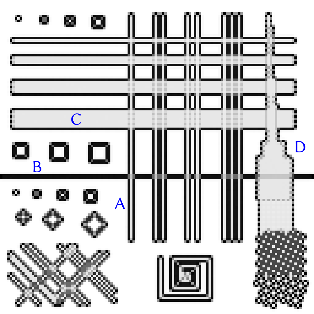
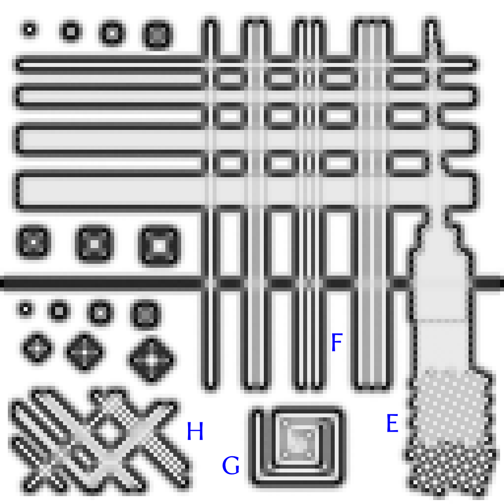
Figure 2: Reference black and white picture (left), stochastic texture differences at spatial scales of $\lambda=1$ (center) and $\lambda=2$ pixels (right), both with value scale $\kappa=0.25$, averaged over 10 independent computations with $n=500$. White stands for a null difference, black for maximum discrepancy. Capital letters markers are commented in the main text.

Some images, like the satellite monitoring of sea surface temperature in Fig. 4, present missing data for some pixels, in this case corresponding to land masses. In that case, entries in some sequences $\left\{s_{i}\right\}_{i\leq m}$ may be missing. We deal with the issue by modifying the kernel to maintain a normalized average over the remaining entries in these sequences:

$$k\left(s,t\right)=1/\left(1+\frac{1}{\left|C\right|}\sum_{i\in C}\left(s_{i}/\kappa-t_{i}/\kappa\right)^{2}\right)$$ (6)

where $C$ is the set of common indices where both sequences have valid entries. When $C=\emptyset$, the kernel value cannot be computed. In that case, we average over remaining kernel evaluations, separately in each term of Eq. 3. When $d\left(S^{-},S^{+}\right)$ cannot be evaluated in some directions $S^{\pm}$, then we average over remaining directions in Eq. 4 to define the texture discrepancy at that pixel. When all directions are invalid, for example in zones of missing data larger than the neighborhood $\boldsymbol{N}^{\pm}(\boldsymbol{o})$, we set the texture discrepancy to Not a Number, indicating missing information. When a large zone of missing data is present, then some directions have to be ignored and textures are compared in the remaining directions. This process adaptatively handles contours of missing data, discarding automatically directions toward missing data and considering only directions tangent to the large invalid zone.

This effect is exploited to deal with pixels at the boundary of an image. Standard techniques for handling such boundaries involve extending border pixel values, mirroring, or setting outside pixel values to zero. However, these methods are only needed to work around the inability of an image processing algorithm to deal with missing data. Since we can, the natural choice for pixels outside the image is to consider them missing. Thanks to the above method, computations at an image border are performed in exactly the same way as for any pixel within the image. Textures to the very border of the image are taken into account and, importantly, without introducing spurious discrepancies (such as setting outside pixels to null would) or spurious similarities (such as mirroring or extending border pixel values would).

IV A scale-dependent texture discrepancy detector

IV-A Demonstration on a synthetic test picture

The synthetic image of Fig. 2 left was designed to demonstrate the behavior of the algorithm on elementary patterns such as one-pixel width lines and chess boards. Labels in Fig. 2 (middle, right) are added for clarity of the discussion. A: points within thin (isolated) 1-pixel lines have the same neighborhood on each side of the line. Points next to these lines have a maximal difference between neighborhoods at 1-pixel scale, resulting in detected edges on each side of the line. At scale 2, points two pixels away also have asymmetric neighborhood, although less than the nearby pixels, hence localization of the maxima is preserved between scales $\lambda=1$ and $\lambda=2$ (for small $\kappa$ values, see Section III-C). B: sharp black/white transitions result in two-pixel wide boundaries, one pixel on each side of the transition, with weaker contributions further away at scale $\lambda=2$. C: lines separated by 1 pixel are fully recognized as being part of the same texture at 1-pixel scale, hence disappear in the stochastic texture difference (STD) maps at scales $\lambda=1$ and $\lambda=2$ . These STD values are nevertheless not null, unlike that of the uniform background, hence these patterns are grayed out instead of blanked out. Boundaries around these texture regions are detected, as in the isolated line case. D: chessboard patterns are also recognized at both scales, together with surrounding edges. The difference between the chessboard pattern and the spaced-out squares below is weakly detected in both cases, while the black/white inversion within the checkboard pattern is only visible at $\lambda=1$. E: this repetitive pattern is better recognized at spatial scale $\lambda=2$ and pixel value scale $\kappa=0.25$ (the average value over a repeating block), but its elements are too isolated at scale $\lambda=1$. The boundaries of that texture are also found at scale $\lambda=2$. Pixels in the region below are too far apart for $\lambda\leq 2$. F: thin lines separated by 2 pixels also become part of the same texture with a surrounding edge at $\lambda=2$, while lines separated by 3 pixels are isolated in both cases. G: The spiral center is a non-repeating pattern of lines 1 pixel apart, which can be recognized at scale $\lambda=2$ (see the black branches within the spiral), while the spiral branches 3 pixels away are still isolated. H: the thin diagonal lines behave similarly than vertical and horizontal lines. Lines too close at either scale are merged into a unified texture with a surrounding edge.

This example clearly demonstrates the effect on changing the spatial scale $\lambda$. The next section also shows the effect of changing the data scale $\kappa$, on a real image presenting both low and large gray scale contrasts.

IV-B Typical behavior of the algorithm on a real image

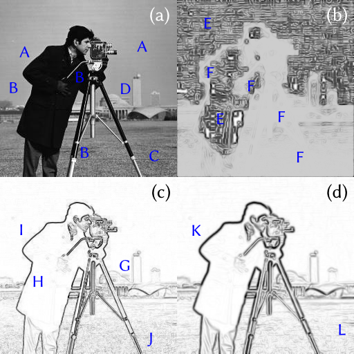
Figure 3: Scale-dependent edge detection. a. Original $256\times 256$ gray scale cameraman image. b. Analysis for $\lambda=3$, $\kappa=1/256$. c. Analysis for $\lambda=1$, $\kappa=1$. d. Analysis for $\lambda=3$, $\kappa=1$. Capital letters markers are commented in the main text.

The effect of analyzing the image at different spatial and data scales is demonstrated is Fig. 3. The classic “cameraman” picture is shown in Fig. 3a. This picture presents jpeg quantization artifacts in the sky region and around the coat (A), large contrasts for the coat, the tripod and the camera handle (B), and fine grass texture with intermediate contrasts (C). Buildings in the background form another medium contrast set (D). At a very low $\kappa=1/256$ of one gray level quantization (Fig. 3b), the STD is sensitive to small changes at that level. Boundaries are detected on jpeg artifacts and within the coat (E). On the other hand, all medium and large gray level gradients $\gg\kappa$ are ignored, as can be seen on the coat edge, camera handle and tripod (F) that have completely disappeared in this picture. The grass texture at intermediate gray level contrasts is also ignored. Conversely, setting $\kappa=1$ in Fig. 3c and Fig. 3d, results in edges that are sensitive to large gray level differences, with the reversed situation of ignoring small gray-level discrepancies. Buildings with intermediate contrast result in intermediate edge values (G). At $\lambda=1$ pixel in Fig. 3c, edges are thin (H) but some jpeg quantization blocs are still faintly visible around the coat (I). This spatial scale is too low for matching the grass texture (J). With a larger $\lambda=3$ pixels in Fig. 3d the edges become smoother (K), but jpeg artifacts are completely gone. Details of the texture finer than $\lambda=3$ are merged (L).

The ability of an STD analysis to focus on specific scales could be very useful, for example, as a filtering guide for artifact removals (low $\kappa$) or for implementing new edge detectors (large $\kappa$).

IV-C Use on physical measuments with characteristic scales

The “cameraman” example demonstrates the ability of the algorithm to analyze and highlight image features at prescribed spatial and data scales. This is especially useful when dealing with physical data, for which processes occur at known scales, independently of the sampling resolution by which that process is measured (i.e. $\lambda$ is better expressed in real units rather than in pixels). As a demonstration, Fig. 4left shows remotely sensed sea surface temperature (s.s.t.), acquired in the infrared band with the MODIS instrument aboard the Terra and Aqua satellites. The covered region ranges from 15°E to 70°E in longitude and 0°S to 60°S in latitude. We use an 8-day composite image in order to remove the cloud cover. Missing data thus correspond to land masses, and is dealt with as described in Section III-D. The floating-point values of the temperature are used as input, from -1.2°C to 31.5°C. The processes we are looking for are oceanic currents, which typically induce a temperature variation of at most a few degrees, so we take a characteristic data scale of $\kappa=1$°C. Their width is variable, between 50-100km, with transitions zones to the surrounding water of a few km, so we take an a priori spatial scale of $\lambda=75$km. Fig. 4right shows the result of the analysis of the sea surface temperature with these parameters, which clearly highlights the dynamics of the ocean at the prescribed scales.

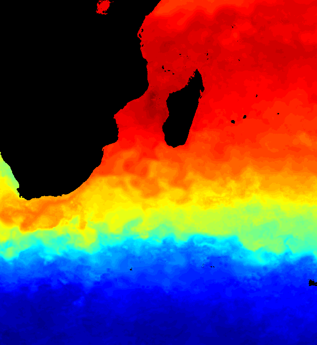
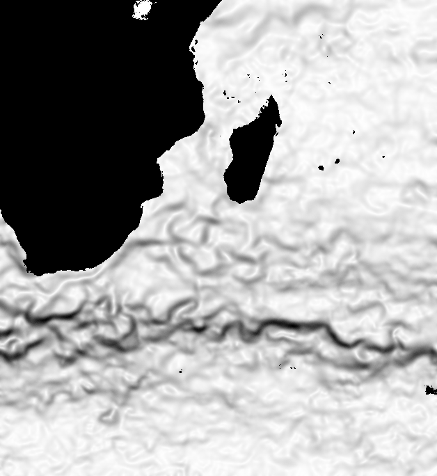
Figure 4: Sea surface temperature. Left: MODIS data, dated 01/01/2006, covering 15°E to 70°E in longitude and 0°S to 60°S in latitude in $628\times 684$ pixels. The floating-point temperature is shown in color scale from blue (-1.2°C) to red (31.5°C). Missing values are shown in black. Right: Analysis with $\kappa=1$°C and $\lambda=75$km (at the center of the picture).

V Multi-scale analysis

V-A Method

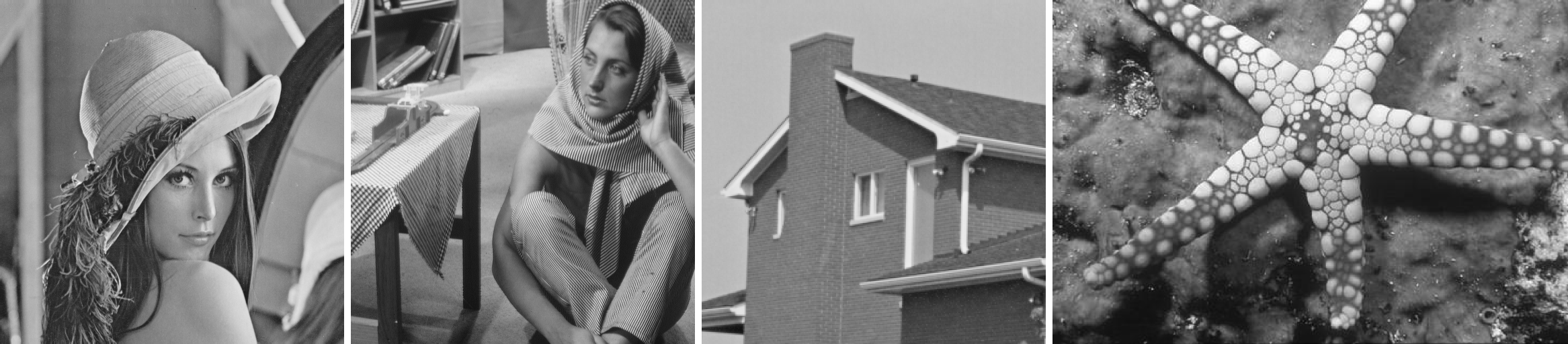
Figure 5: Classic reference images. From left to right, lena, barbara, house and sea star. We use the versions of lena, barbara and house from [41]. The sea star picture is the training example 12003 from the Berkeley segmentation data set [6]. We choosed it as it presents some background texture with higher intensity spots, some blurry and some sharp edges.

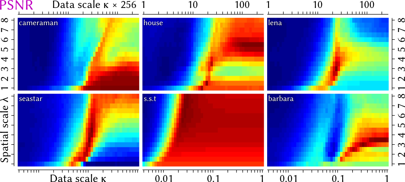
Figure 6: Influence of the two scale parameters $\lambda$ and $\kappa$ on the reconstruction accuracy, measured with the peak signal to noise ratio (PSNR) as defined in the main text, when retaining 20% of the points with higher STD. Averages of 5 independent computations with $n=100$ were used for computing the PSNR. The minimum and maximum values for the PSNR are given in Table I, for each image. Using these per-image bounds, blue is the lowest accuracy, red the highest. The spatial scale $\lambda$ is given in pixels, the data scale $\kappa$ is given for $[0..1]$-normalized data values. An additional scale $\kappa\times 256$ is shown on the top to ease the interpretation of gray-scaled image results. Conversion factors for the sea surface temperature data are $\kappa\approx 0.03$ for $1$°C and $\lambda\approx 1$ pixel for $8.46$ km at the center of Fig. 4.

The previous section presents the case where scales are chosen a priori, according to the user’s knowledge or objectives. But such information is not always available: in many cases, the goal is precisely to find what are the relevant scales to describe a data set. We thus need a methodology to identify which are the “best” scales in an image, with objective measurement criteria.

One hypothesis is that the “best” scales should identify correctly the most relevant structures in a data set, which we identify with the structures carrying most of the information. Assuming this is the case, then we propose the following methodology:

– Analyze the data for a given pair of scales $\lambda$ and $\kappa$.

– Select the 20% most discriminative points, taken to be pixels $\boldsymbol{x}$ with the largest $d(\boldsymbol{x})$ STD values.

– Reconstruct the image from only these points, according to the method detailed below.

– Compare the reconstructed image with the original.

If the features are correctly determined and they indeed carry most of the information on the image, then the reconstruction should be very close to the original. This procedure can also be seen as a lossy compression of an image: information in the discarded pixels is lost and these are reconstructed from the retained pixels. Perfect features holding all the information would mean perfect restoration of the image after decompression. We emphasize that our goal is not to obtain the largest PSNR from the minimum number of retained points, which is related topic adressed by other works in the litterature [35]. Rather, we wish to use the simplest method, so that the reconstruction accuracy measures the sole influence of $\lambda$ and $\kappa$, and not their joint effect with reconstruction methods designed to improve the PSNR. This excludes anisotropic diffusion [36], weighting [37], exploiting dictionaries [38], etc.

Reconstruction is thus performed by minimizing a least square error, equivalent to solving a Poisson Equation [39, 40]. More precisely, considering all pairs of neighbor valid pixels $\boldsymbol{a}$ and $\boldsymbol{b}$ (i.e. both are within image boundaries and without missing data), we seek the reconstructed image $\boldsymbol{J}$ with pixel values $v_{\boldsymbol{J}}\in\mathcal{V}$ such that:

$$\boldsymbol{J}=\left\{v_{\boldsymbol{J}}:\,\min\sum_{\boldsymbol{a},\boldsymbol{b}}\left(v_{\boldsymbol{J}}(\boldsymbol{b})-v_{\boldsymbol{J}}(\boldsymbol{a})-g(\boldsymbol{a},\boldsymbol{b})\right)^{2}\right\}$$ (7)

Here $g(\boldsymbol{a},\boldsymbol{b})=v_{\boldsymbol{I}}(\boldsymbol{b})-v_{\boldsymbol{I}}(\boldsymbol{a})$ is the gradient of the original image $\boldsymbol{I}$ whenever pixel $\boldsymbol{a}$ is retained amongst the 20% with largest STD value, and null otherwise. This reconstruction is unique, optimal in the least square sense, and does not introduce any extra processing step on the image. It can be computed simply with sparse optimizers, such as [34]. We then add the mean of the original image that was lost in the process before comparing $\boldsymbol{J}$ and $\boldsymbol{I}$, and clamp pixels within the normalized $[0,1]$ interval.

In order to assert the quality of the reconstruction, we use the Peak Signal to Noise Ratio (PSNR) criterion, as defined by:

$$\textrm{PSNR}\left(\boldsymbol{I},\boldsymbol{J}\right)=10\log_{10}\left(\left|C\right|/\sum_{\boldsymbol{a}\in C}\left(v_{\boldsymbol{I}}(\boldsymbol{a})-v_{\boldsymbol{J}}(\boldsymbol{a})\right)^{2}\right)$$

where $C$ is the set of common valid pixels in $\boldsymbol{I}$ and $\boldsymbol{J}$.

V-B Results

In addition to the cameraman and sea surface temperature images, we also analyze the “lena”, “barbara”, “sea star” and “house” images, shown in Fig. 5. Their multiscale analysis maps are shown in Fig. 6 and the PSNR maxima are given in Table I. Scales leading to better global reconstructions are clearly visible, forming distinct patterns for every picture.

Table I: Reconstruction accuracy when retaining 20% of the points and best scales for the test images.

Image	Best $\lambda$	Best $\kappa$	min PSNR	max PSNR
cameraman	1	0.41	12.0	28.3
house	5.5	0.64	13.5	26.2
lena	3	0.094	13.6	21.0
seastar	3.5	0.11	13.7	18.2
s.s.t.	7	0.027	10.8	23.9
barbara	3.5	0.64	13.0	17.7

Our method provides a new multi-scale analysis of an image, in order to highlight the characteristic spatial $\lambda$ and data $\kappa$ scale of its components. For example, we can see that the house picture has a maxima zone at $\lambda=5$ to $6$ and high $\kappa$: this corresponds to the spatial extent and the contrast difference of the white borders of the roof, window frames and water drain. Other maxima are located at $\lambda$ of $1$ and $1.5$ pixels, with medium $\kappa$ gray scale contrast: these are the brick textures. With this method, automatically identified parameters for the sea surface temperature data are $\lambda\approx 59$km and $\kappa\approx 0.9$°C. These are consistent with our a priori estimate in Sec. IV-C, further validating our approach.

V-C Selective texture erasing

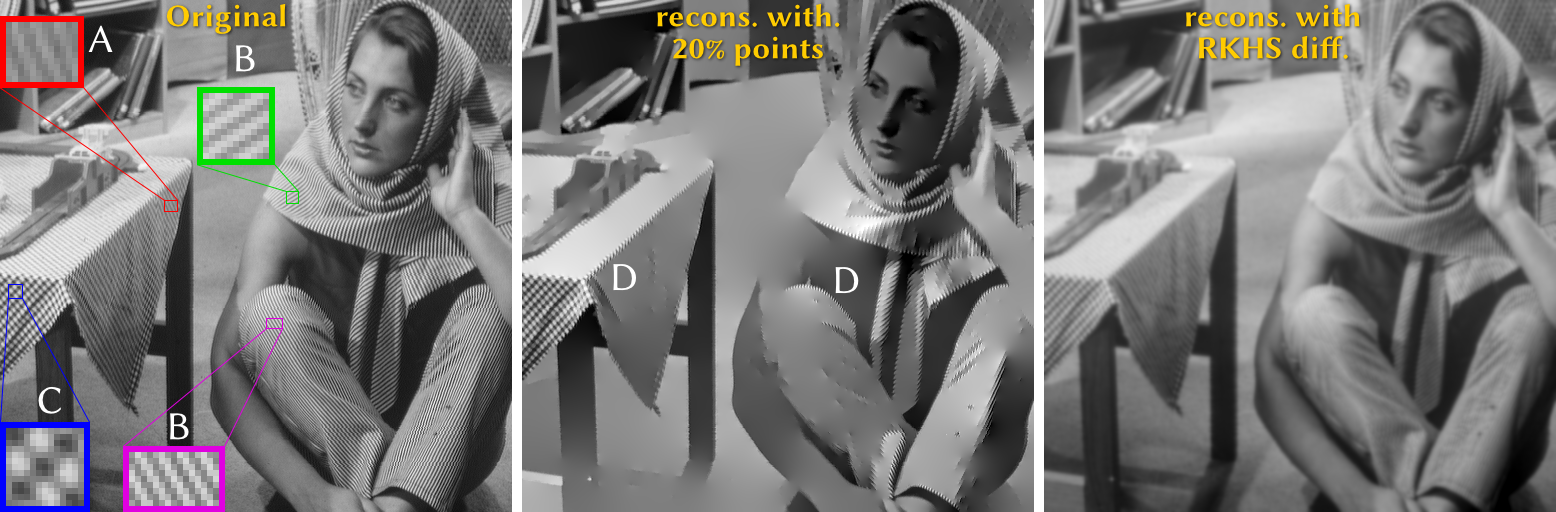
Figure 7: Erasing texture elements smaller than $\lambda=3.5$ pixels. Left: Annotated original Barbara image. Middle: Reconstruction from 20% selected points at $\lambda=3.5$ and $\kappa=0.64$, corresponding to the maximum of Table I. Right: Reconstruction with 100% points but using the RKHS “texture gradient” instead of the image gradient.

Similarly, the stripped patterns of the Barbara image are correctly matched on both scales. Fig. 7 shows in region A a texture of slanted stripes with a characteristic size $\lambda<2.5$ and a low gray level constrast $\kappa$. These textures are correctly detected in the PSNR map of Fig. 6 as the leftmost maxima with lower $\lambda$ values. But the image also comprises other patterns of increasing contrast and size, as can be seen in regions B. Most of them have a characteristic size $\lambda=3.5$, at which the PSNR reaches a maxima for a range of large gray scales $\kappa$.

Fig. 7 (middle) shows that textures disappear in the reconstructed image from the 20% largest STD pixels. Some patterns, like in region C, present textures with a larger spatial extent. As was the case for the artificial image in section 2, these patterns are not recognized with a smaller $\lambda=3.5$, and they appear intact in the reconstruction. Our method can thus also be used for texture erasing [42, 43], preserving edges between different regions and around textured elements (D) but selectively removing all textures below a prescribed spatial scale $\lambda$.

An alternative method is to seek the image with gradients (Eq. 7) that are as close as possible to the texture difference values (Eq. 3). Since there cannot be a linear correspondance between pixel gradients in image space and “texture gradients” in RKHS, involving a non-linear reproducing kernel, it is expected that distortions are produced in the reconstructed image, assuming a meaningful image can be produced in the first place. Technical details for how to combine Eq. 3 into Eq. 7 are given in Appendix C, and involve orienting the “texture gradient” with the average intensity on each side of a target pixel. Despite being necessarily imperfect, Fig. 7 (right) shows that a reconstruction can still be obtained this way, with a PSNR of 22.95 and erased textures below $\lambda$, but with some amount of blurring. The interesting point is that the method works as intended, proving that our “texture gradient” operation in RKHS, when properly oriented, really behaves like a gradient.

VI Color texture differences

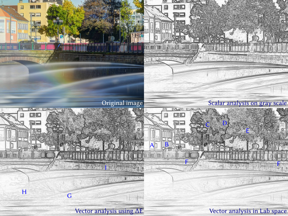
Figure 8: Texture difference analysis of a color image. Top-left: original image (full credit given in Appendix), rescaled to 600x450 pixels. Top-right: Scalar analysis using a gray version of the image. Bottom-right: Vector analysis in Lab space with the standard D65 white point. Bottom-left: Vector analysis using the CIE DE2000 perceptual color difference improvement $\Delta E$. All these analyses use the spatial scale $\lambda=1.5$ pixels and the data scale $\kappa=0.15$.

The path generation procedure described in Section III-A makes no assumption on the nature of pixel values $v\in\mathcal{V}$, just that sequences $t\in\mathcal{V}^{m}$ can be compared with a suitable reproducing kernel. The case for scalar pixels is presented above, but the method works equally well on vector data. In this case, $\mathcal{V}$ could be a color space, a set of spectral bands in remote sensing applications, polarized synthetic aperture radar values, or any other vector data. We deal here with the most common case of a triplet of RGB values. We first consider a kernel $k:\,\mathcal{V}\times\mathcal{V}\rightarrow\mathbb{R}$ that compares two RGB triplets and produce a similarity value, then take the product space kernel in $\mathcal{V}^{m}$ for comparing sequences.

Specifically, assuming $\mathcal{V}$ is the set of all $v=\left(R,G,B\right)$ triplets, we first consider the non-linear conversion operator $\ell:\,\mathcal{V}\rightarrow\mathcal{L}$ to the CIE Lab space $\mathcal{L}$ using the standard D65 white point. $\ell(v)$ is thus a vector with entries $\left(L,a,b\right)$. Then, we implement the following color difference operators:

– $\delta_{1}\left(v,w\right)=\left\|\ell\left(v\right)-\ell\left(w\right)\right\|_{\mathcal{L}}/100$, based on the original intent of the Lab space to be perceptually uniform, so the norm in $\mathcal{L}$ should match a perceived color difference. This first formula is fast to compute.

– $\delta_{2}\left(v,w\right)=\Delta E\left(\ell\left(v\right),\ell\left(w\right)\right)/100$, based on the revised CIE DE 2000 standard [44] for producing a better perceptually uniform difference $\Delta E$ between two Lab triplets. This second formula is slower to compute, but presumably more accurate.

The kernel between two sequences $s,t\in\mathcal{V}^{m}$ is then easily adapted from Eq. 6, with the same notations:

$$k_{d}\left(s,t\right)=1/\left(1+\frac{1}{\left|C\right|}\sum_{i\in C}\left(\delta_{d}\left(s_{i},t_{i}\right)/\kappa\right)^{2}\right)\mbox{ with }d=1,2$$ (8)

The data scale $\kappa$ is now applied to the chosen $\delta_{1}$ or $\delta_{2}$ operator, in order to highlight small or large color differences. Note that we normalize $\delta_{1}$ and $\delta_{2}$ to be within $\left[0\ldots 1\right]$ instead of the $\left[0\ldots 100\right]$ Lab space range, so that $\kappa$ values for the color case are comparable to the scalar case presented in the previous sections: assuming the gray scale perfectly matches a perceptual color intensity, then $\kappa$ would have the same meaning in the color and the gray scale analysis. Using the same normalized $\kappa$, the scalar and vector analysis in Fig. 8 are thus expected to have a similar, but not exactly identical, general contrast range. On the other hand, the CIEDE2000 $\Delta E$ formula was designed to correct slight discrepancies in the original Lab space perceptual uniformity, hence the contrast levels of the two vector analysis should be very similar, with only minor changes due to the $\Delta E$ correction. This is what we observed in Fig. 8.

Fig. 8 shows how the vector analysis, using either the Lab space norm or $\Delta E$ for color matching, enhances the detected features compared to the scalar analysis on gray scale. In region A, the color difference in the top-left of the trompe-l’œil painting is well recognized in the vector analysis, but the contrast is not large enough in gray scale. The real wall and windows on the same house (B) are also much better analyzed in color, especially with the orange/beige difference. Another prominent difference is the lamp post (C) in front of the tree, which is lost in foliage details in the gray scale version but clearly contoured in the color analysis. Unlike points A and B, this effect is not only due to color contrast, but it also involves the texture difference between the lamp post and the tree foliage. Texture differencing between the two trees is clearly visible in D, where the green tree is well contoured in the color analysis, while both trees have similar textures in gray scale. The small patchs of blue sky (E) better stand out against more uniform foliage textures in the color versions, compared to the gray case where they are buried in noise. Color panels are also better recognized in F. The rainbow is not detected (G) by any of the analyses. But its slowly varying colors over a large spatial extent do not match the scales $\lambda=1.5$ pixels and $\kappa=0.15$ that are used here.

The effect of using the CIEDE2000 correction is visible by close inspection of the bottom images in Fig. 8. Compared to the original Lab space, the non-linear $\Delta E$ correction gives slightly more contrast to the lower color differences, which was one of its purposes in the first place [44]. These effects are visible throughout the image, but maybe more clearly seen on the water (H) and stone wall (I) texture details. However, these effects are so small that, for most applications, computing $\Delta E$ may not be worth the added cost compared to working in the original Lab space.

In any case, our method provides a new way to include color information in image and texture analysis, highlighed especially by points A, B and C above. More generally, the method is applicable whenever a reproducible kernel can be defined to compare pixel elements, whether these are scalar, vector, strings, graphs, etc.

VII Conclusion

We introduce a new low-level image analysis method, based on statistical properties within the neighborhood of each pixel. We have demonstrated its use on synthetic and real images. In particular, our algorithm is able to retreive characteristic scales in remotely sensed data. The method we present is not limited to scalar values and it is readily applicable to any kind of data for which a reproducing kernel is available. This includes vector data, and in particular color triplets. Thanks to being specified at prescribed spatial and data scales, our method implements a new kind of filter, very different from wavelet-based analysis [9] or decomposition on dictionaries [12]. For example, it can detect small discrepancies like jpeg quantization artifacts while being insensitive to large luminosity gradients, which could be useful for guided filtering of these artifacts. In the spatial domain, our method can detect repetitive texture patterns, as shown in Figs. 2 and 7, and produces a unique contour around these elements. This low-level algorithm represents textures in a statistical framework that is quite different from classic approaches like textons [13], and it also represents multi-scale information in a new framework. Our new method thus complements these techniques, and together with them has the potential to provide really new feature descriptors for images, with properties that need to be explored in future works.

Appendix A: Producing texture discrepancy for missing data

For directions tangent to an invalid data zone, half the neighborhood is valid and half is invalid, in both $S^{+}$ and $S^{-}$(at worst, since $\boldsymbol{N}^{\pm}(\boldsymbol{o})$ is centered on the center of the valid pixel $\boldsymbol{o}$, not on the edge). For such a $S^{\pm}$ pair, and replacing the neighborhood by another worst-case approximation of a binary valid/invalid choice (i.e. neglecting $m$ and the spatial extent $\lambda$ with many valid pixels in the neighborhood), the probability of never selecting a valid pair of pixels decreases exponentially as $O(2^{-n^{2}})$ according to Eq. 3, tending to null probability in the large $n$ limit. For a typical computation with $n=100$, this a gives ridiculously small $p<10^{-3000}$ probability of an invalid result. Thus, for all practical purposes, valid pixels near an invalid boundary “always” produce a valid computation result for typical and small values of $n$.

In fact, even missing pixels within large missing data zones benefit from nearby valid pixels. Although we explicitly ignore these STD values due to their low accuracy, our method still allows getting relevant values for isolated missing pixels. Consider a neighborhood centered on that pixel. In that case, paths around that point may occasionally fall onto the missing pixel, but patterns are still matched outside that pixel. Since the modified kernel is normalized only on valid pixels, the missing data simply results in a reduction of the effective $m=\left|C\right|$, but valid patterns surrounding the missing pixel are still matched correctly in every direction. The price to pay is a loss of reliability, especially as the nearest distance to a valid pixel grows. We do not exploit this feature in the data presented in the main text, where no STD value is produced for missing pixels, but this feature could be useful in other contexts, for example to simply ignore isolated missing pixels.

Appendix B: Combining scales

In Section III-C, $\kappa$ sets the scale at which scalar pixel values are compared and should reflect a priori information on the image. In order to compare probability distributions, [27] proposes to either take a Bayesian approach for letting $\kappa$ vary with a priori knowledge, or to take $d\left(S^{-},S^{+}\right)=\sup_{\kappa}\,d_{\kappa}\left(S^{-},S^{+}\right)$ over a range of $\kappa$ for a more systematic approach. We found that the latter does not perform well in practice. For example, a picture captured by a digital camera sensor in low light conditions presents some digital noise on the pixel values. A similar effect occurs for quantization noise and jpeg artifacts (see Section IV-B). Comparing distributions in $\mathcal{V}^{m}$ at the scale of this noise is meaningless, as it would reflect differences due to the sensor (resp. quantization algorithm) itself, but not the differences in the image textures. Given the sensor fluctuations, the distance $d_{\kappa}\left(S^{-},S^{+}\right)$ at low $\kappa$ values is larger that at the natural scale of the image signal, hence the $\sup_{\kappa}$ approach does not work in this case. Physically, and for remotely sensed data in particular, the $\sup_{\kappa}$ approach amounts to mixing together processes at different characteristic scales, which may have nothing to do with each other.

Appendix C: Reconstruction from “texture gradients”

For a pair of valid neighbor pixels $(\boldsymbol{a},\boldsymbol{b})$, consider the neighborhood $\boldsymbol{N}^{+}(\boldsymbol{a})$ that includes $\boldsymbol{b}$ and $\boldsymbol{N}^{-}(\boldsymbol{b})$ that includes $\boldsymbol{a}$. We add constraints in Eq. 7 using Eq. 3 for the gradients: $\min\sum_{\boldsymbol{a},\boldsymbol{b}}\left(v_{\boldsymbol{J}}(\boldsymbol{b})-v_{\boldsymbol{J}}(\boldsymbol{a})\pm d\left(S^{-}(\boldsymbol{a}),S^{+}(\boldsymbol{a})\right)\right)^{2}+\left(v_{\boldsymbol{J}}(\boldsymbol{b})-v_{\boldsymbol{J}}(\boldsymbol{a})\pm d\left(S^{-}(\boldsymbol{b}),S^{+}(\boldsymbol{b})\right)\right)^{2}$. The signs are determined using the average value of the original image pixels in each neighborhood: $\mbox{{sign}\,}d\left(S^{-}(\boldsymbol{a}),S^{+}(\boldsymbol{a})\right)=\textrm{sign}\left(\sum_{\boldsymbol{x}\in\boldsymbol{N}^{+}(\boldsymbol{a})}p(\boldsymbol{x})v_{\boldsymbol{I}}(\boldsymbol{x})-\sum_{\boldsymbol{x}\in\boldsymbol{N}^{-}(\boldsymbol{a})}p(\boldsymbol{x})v_{\boldsymbol{I}}(\boldsymbol{x})\right)$, and similarly for $\boldsymbol{b}$. With this method, the result for $\lambda=3.5$ and $\kappa=0.64$ is shown in Fig. 7 right.

Appendix D: Data and code availability

The code used in this paper is free software, available for download at https://gforge.inria.fr/scm/?group_id=5803. Images for Lena, Barbara, house, were fetched from J. Portilla’s web page and match these used in [41]. We used the cameraman picture from McGuire Graphics Data at http://graphics.cs.williams.edu/data/images.xml. The sea star is the training sample 12003 from the Berkeley segmentation S300 data set [6] and was downloaded from http://www.eecs.berkeley.edu/Research/Projects/CS/vision/bsds/BSDS300/html/dataset/images/gray/12003.html. The sea surface temperature data was provided by the Legos laboratory http://www.legos.obs-mip.fr/. The color image in Fig. 8 comes from Wikimedia Commons, at http://commons.wikimedia.org/wiki/File:2013-10-19_10-53-16-savoureuse-belfort.jpg. This long exposure photograph was taken by Thomas Bresson with a polarizing filter, and released under Creative Commons - Attribution - 3.0. The original image was cropped and resized to $600\times 450$ pixels.

References

- [1] Leo Grady, “Random Walks for Image Segmentation”. IEEE Transactions on pattern analysis and machine intelligence 28(11), pp. 1768–1783, (2006).
- [2] Vincenzo Nicosia, Manlio De Domenico and Vito Latora, “Characteristic exponents of complex networks”. Europhysics Letters 106(5), 58005, (2014).
- [3] Xiaofeng Ren, Liefeng Bo, “Discriminatively Trained Sparse Code Gradients for Contour Detection”. Advances in Neural Information Processing Systems proceedings, 2012.
- [4] Jianbo Shi, Jitendra Malik, “Normalized Cuts and Image Segmentation”. IEEE transactions on Pattern Analysis and Machine Intelligence 22(8), pp. 888-905, (2000).
- [5] Michael Maire, Pablo Arbeláez, Charless Fowlkes, Jitendra Malik, “Using Contours to Detect and Localize Junctions in Natural Images”, IEEE Conference on Computer Vision and Pattern Recognition proceedings, (2008).
- [6] D. Martin, C. Fowlkes, D. Tal, J. Malik, “A Database of Human Segmented Natural Images and its Application to Evaluating Segmentation Algorithms and Measuring Ecological Statistics”. Proc. 8th Int’l Conf. Computer Vision, vol. 2, pp. 416–423, (2001).
- [7] J. Zhang, M. Marszałeck, S. Lazebnik, C. Schmid, “Local Features and Kernels for Classification of Texture and Object Categories: A Comprehensive Study”. International Journal of Computer Vision 73(2): 213-238 (2007).
- [8] K. Jafari-Khouzani, H. Soltanian-Zadeh, “Rotation-Invariant Multiresolution Texture Analysis Using Radon and Wavelet Transforms”. IEEE Transactions on Image Processing 14(6): 783-795 (2005).
- [9] Jean-Luc Starck, Emmanuel J. Candès, and David L. Donoho, “The Curvelet Transform for Image Denoising”, IEEE Transactions on Image Processing 11(6), pp. 670-684, (2002).
- [10] E. Le Pennec , S. Mallat , “Bandelet Image Approximation and Compression”, Journal of Multiscale Modeling and Simulation 4(3), pp. 992-1039, 2005.
- [11] M.N. Do, M. Vetterli, “The contourlet transform: an efficient directional multiresolution image representation”. IEEE Transactions on Image Processing 14(12): 2091-2106 (2005).
- [12] Julien Mairal, Francis Bach, Jean Ponce, Guillermo Sapiro, Andrew Zisserman, “Discriminative Learned Dictionaries for Local Image Analysis”, IEEE Conference on Computer Vision and Pattern Recognition proceedings, (2008).
- [13] Jitendra Malik, Serge Belongie, Thomas Leung, Jianbo Shi, “Contour and Texture Analysis for Image Segmentation”. International Journal of Computer Vision 43(1), pp. 7-27, (2001).
- [14] H. Badri, H. Yahia, K. Daoudi, “Fast and Accurate Texture Recognition with Multilayer Convolution and Multifractal Analysis”, European Conference on Computer Vision (ECCV) proceedings, pp. 505-519 (2014).
- [15] Y. Xia, D.D. Feng, R. Zhao, “Morphology-based multifractal estimation for texture segmentation”. IEEE Transactions on Image Processing 15(3): 614 - 623 (2006).
- [16] Tony Lindeberg, “Scale-space theory: A basic tool for analysing structures at different scales”, Journal of Applied Statistics 21(2), pp. 225-270, (1994).
- [17] Tony Lindeberg, “Edge detection and ridge detection with automatic scale selection”, International Journal of Computer Vision, 30(2), pp. 117-156, (1998).
- [18] Stella X. Yu, “Segmentation Induced by Scale Invariance”, IEEE Conference on Computer Vision and Pattern Recognition proceedings, (2005).
- [19] U. Braga-Neto, J. Goutsias, “Grayscale Level Connectivity: Theory and Applications”. IEEE Transactions on Image Processing 13(12): 1567-1580 (2004).
- [20] S. Konishi, A. Yuille, J. Coughlan, “A statistical approach to multi-scale edge detection”. Image and Vision Computing 21(1): 37-48 (2003).
- [21] Schmidt, U. ; Dept. of Comput. Sci., Tech. Univ. Darmstadt, Darmstadt, Germany ; Qi Gao ; Roth, S., “A generative perspective on MRFs in low-level vision”. IEEE Conference on Computer Vision and Pattern Recognition (CVPR), 2010
- [22] K-H. Liang, T. Tjahjadi, “Adaptive Scale Fixing for Multiscale Texture Segmentation”. IEEE Transactions on Image Processing 15(1): 249-256 (2006).
- [23] P. Perona and J. Malik, “Scale-space and edge detection using anisotropic diffusion”. IEEE Transactions on Patern Analysis and Machine Intelligence, 12: 629-639 (1990).
- [24] A. Petrovic, O. D. Escoda, P. Vandergheynst, “Multiresolution Segmentation of Natural Images: From Linear to Nonlinear Scale-Space Representations”. IEEE Transactions on Image Processing 13(8): 1104-1114 (2004).
- [25] X. Dong, I. Pollak, “Multiscale Segmentation With Vector-Valued Nonlinear Diffusions on Arbitrary Graphs”. IEEE Transactions on Image Processing 13(8): 1104-1114 (2004).
- [26] C. Fernandez-Lozano, J. A. Seoane, M. Gestal, T. R. Gaunt, C. Campbell, “Texture Classification Using Kernel-Based Techniques”. Lecture Notes in Computer Science 7902: 427-434 (2013).
- [27] Bharath K. Sriperumbudur, Arthur Gretton, Kenji Fukumizu, Bernhard Schölkopf, Gert R. G. Lanckriet, “Hilbert Space Embeddings and Metrics on Probability Measures”. Journal of Machine Learning Research 11, pp. 1517-1561, (2010).
- [28] Arthur Gretton, Karsten M. Borgwardt, Malte J. Rasch, Bernhard Schölkopf, Alexander Smola, “A Kernel Two-Sample Test”. Journal of Machine Learning Research 13, pp. 723-773, (2012).
- [29] D.R. Martin, C. C. Fowlkes, J. Malik, “Learning to Detect Natural Image Boundaries Using Local Brightness, Color, and Texture Cues”. IEEE Transactions on Patern Analysis and Machine Intelligence 26(1): 530-549 (2004).
- [30] M. Clerc, S. Mallat, “The Texture Gradient Equation for Recovering Shape from Texture”. IEEE Transactions on Patern Analysis and Machine Intelligence 24(4): 536-549 (2002).
- [31] J. Angulo. “Morphological texture gradients. Application to colour+texture watershed segmentation”. Proceedings of the 8th International Symposium on Mathematical Morphology (ISMM2007), pp. 363-374, 2007.
- [32] R.J. O’Callaghan, D.R. Bull, “Combined morphological-spectral unsupervised image segmentation”, IEEE Transactions on Image Processing 14(1):49-62 (2005)
- [33] [3] John Canny, “A computational approach to edge detection”. IEEE transactions on Pattern Analysis and Machine Intelligence 8(6), pp. 679-698 (1986).
- [34] S. Agarwal, K. Mierle and Others, “Ceres Solver”, http://ceres-solver.org (source code fetched 04 February 2015).
- [35] W. Dong, G. Shi, X. Li, “Nonlocal Image Restoration With Bilateral Variance Estimation: A Low-Rank Approach”. IEEE transactions on image processing 22(2): 700-711 (2013).
- [36] S. K. Maji, H. M. Yahia, “Edges, transitions and criticality”. Pattern Recognition 47: 2104-2115 (2014).
- [37] A. Agrawal, R. Raskar, R. Chellappa, “What is the Range of Surface Reconstructions from a Gradient Field?”. Computer Vision – ECCV proceedings in Lecture Notes in Computer Science 3951: 578-591 (2006).
- [38] M. Aharon, M. Elad, A. Bruckstein, “K-SVD: An Algorithm for Designing Overcomplete Dictionaries for Sparse Representation”, IEEE transactions on image processing 54(11): 4311-4322 (2006).
- [39] T. Simchony, R. Chellappa, M. Chao, “Direct analytical methods for solving Poisson equations in computer vision problems”. IEEE transactions on pattern analysis and machine intelligence 12 (5): 435-446, 1990.
- [40] S. K. Maji, H. M. Yahia, H. Badri, “Reconstructing an image from its edge representation”. Digital Signal Processing 23: 1867–1876 (2013).
- [41] J Portilla, V Strela, M Wainwright, E P Simoncelli, “Image Denoising using Scale Mixtures of Gaussians in the Wavelet Domain”. IEEE Transactions on Image Processing. vol 12, no. 11, pp. 1338-1351, (2003).
- [42] P. Pérez, M. Gangnet, A. Blake, “Poisson Image Editing”, ACM Transactions on Graphics, 22(3): 313-318 (2003).
- [43] L. Xu, C. Lu, Y. Xu, J. Jia, “Image Smoothing via L0 Gradient Minimization”. ACM Transactions on Graphics, SIGGRAPH Asia, 30 (5) (2011).
- [44] G. Sharma, W. Wu, E. N. Dalal, “The CIEDE2000 color-difference formula: Implementation notes, supplementary test data, and mathematical observations”. Color Research & Applications (Wiley Interscience) 30 (1): 21–30 (2005).
- [45] C. Lu, L. Xu, J. Jia, “Contrast Preserving Decolorization”. IEEE International Conference on Computational Photography (ICCP), (2012).