Frequency comb generation beyond the Lugiato-Lefever equation: multi-stability and super cavity solitons

Abstract

The generation of optical frequency combs in microresonators is considered without resorting to the mean-field approximation. New dynamical regimes are found to appear for high intracavity power that cannot be modeled using the Lugiato-Lefever equation. Using the Ikeda map we show the existence of multi-valued stationary states and analyse their stability. Period doubled patterns are considered and a novel type of super cavity soliton associated with the multi-stable states is predicted.

I Introduction

The generation of optical frequency combs using microresonator devices is currently a hot topic that is attracting a significant amount of research. A mode-locked optical frequency comb can combine an ultra broadband spectrum with coherent and finely resolved comb lines at an equidistant frequency spacing. Microresonator based optical frequency combs have a plethora of potential applications in, e.g., the areas of precision metrology, spectroscopy, optical clocks, wavelength-division multiplexing sources, and arbitrary waveform generation kippenberg_microresonator-based_2011 . By enclosing a nonlinear medium within a resonator structure, a wealth of dynamical behaviours appear. Microresonators with a Kerr nonlinearity that are pumped by a continuous wave (CW) laser are known to support bistable CW solutions, as well as both periodic temporal (Turing) patterns and localised cavity soliton solutions. These solutions may be either stable or unstable, depending on the operating regime determined by the power and detuning of the pump laser. Additionally, there exist operating regimes where the intracavity field is chaotic.

Previous work on the generation of optical frequency combs in microresonator devices has primarily focused on the regime where the intracavity power is relatively low. In this case the mean-field approximation is valid, and the dynamics can be accurately modeled using either the Lugiato-Lefever equation (LLE) lugiato_spatial_1987 or using the theory of coupled mode equations coen_modeling_2013 ; chembo_modal_2010 . For these approaches to be applicable, it is assumed that the overall cavity detuning, including both linear and nonlinear contributions, remains small during propagation. Particularly, it is assumed that the characteristic nonlinear length scale is much longer than the path length of the cavity. In the present work, we aim to go beyond the LLE and the mean-field approximation, and consider the resonator dynamics when the nonlinear phase-shift is relatively large (of the order of unity).

As a motivation for why it might be prudent to consider microresonator dynamics beyond the LLE, we note that mean-field models have been unable to account for the complete range of dynamical behaviours that have been experimentally observed in resonator devices. Recent experimental work at NIST has e.g. shown examples of frequency combs that are not well described by the LLE delhaye_phase_2015 . Mean-field models are also unable to account for the period doubling behaviour, which has been observed to occur in dissipative fiber-ring resonators nakatsuka_observation_1983 ; temporal_valle_1991 ; coen_experimental_1998 . This period doubling behaviour is distinct from the periodic breathing of cavity soliton type solutions of the LLE, which occurs on a different time-scale that is not associated with the roundtrip time. Period doubling in fiber-ring cavities has been experimentally observed in the periodic switching of the amplitude of output pulses when a fiber-ring resonator is pumped by a synchronised pulse train with large input amplitude temporal_valle_1991 . The period doubling sequence is also well known to be an essential component in the route to chaos nakatsuka_observation_1983 ; Ankiewicz_chaos_1987 .

While the lengths of microresonators are generally about four or so orders of magnitude shorter than fiber-ring resonators, they can display nonlinearities that are several orders of magnitude greater than the $\chi^{(3)}$ nonlinearity of silica fiber. This is especially true for microring resonators made of semiconductor materials. The use of highly nonlinear microring resonators with fairly long path lengths, in combination with intense input pump powers, could consequently enable the observation of microresonator dynamics similar to what has previously been observed in fiber-ring resonators.

In the next section II we introduce the Ikeda map, which is the basic model system used to describe frequency comb generation beyond the LLE. We use the Ikeda map to analyse the CW solution in section III and show that additional stationary states with higher intracavity power appear when compared to the LLE. The stability of these stationary states is investigated in section IV, showing the presence of new parametric instabilities other than the conventional modulational instability for high pump powers. In Section V we use the parametric instability to show examples of period doubling behaviour. Thereafter, in section VI, we demonstrate the intriguing possibility of forming super energetic cavity soliton associated with the excited states. Finally, in the last section VII, we summarise the article and present some overall conclusions.

II The Ikeda map

In this section we introduce the Ikeda map ikeda_multiple-valued_1979 , which we use to model the dynamics of optical frequency combs without resorting to the mean-field approximation. The map is constructed by combining an ordinary nonlinear Schrödinger equation, for describing the evolution of the envelope of the electric field within a waveguide, together with boundary conditions that relate the fields between successive roundtrips and the input pump field haelterman_dissipative_1992 ; coen_modeling_2013 , viz.

$$E^{m+1}(t,0)=\sqrt{\theta}E_{in}+\sqrt{1-\theta}e^{i\phi_{0}}E^{m}(t,L),$$ (1)

$$\frac{\partial E^{m}(t,z)}{\partial z}=-\frac{\alpha_{i}}{2}E^{m}(t,z)-i\frac{\beta_{2}}{2}\frac{\partial^{2}E^{m}(t,z)}{\partial t^{2}}$$

$$+i\gamma|E^{m}(t,z)|^{2}E^{m}(t,z).$$ (2)

Here the independent variables are the evolution variable $z$, which is the longitudinal coordinate measured along the waveguide and $t$ which is the (ordinary) time. The first equation is the boundary condition that determines the intracavity field $E^{m+1}(t,z=0)$ at the input of roundtrip $m+1$ in terms of the field from the end of the previous roundtrip $E^{m}(t,z=L)$ and the pump field $E_{in}$. The path length of the resonator is assumed to be equal to $L$. Additionally, $\theta$ is the coupling transmission coefficient and $\phi_{0}=2\pi l-\delta_{0}$ is the linear phase-shift, with $\delta_{0}$ the frequency detuning from the cavity resonance closest to the pump frequency, assumed to correspond to the longitudinal mode number $l=0$. Eq.(2) is written in the reference frame moving at the group velocity, with second-order group velocity dispersion coefficient $\beta_{2}$ and nonlinear coefficient $\gamma=n_{2}\omega_{0}/(cA_{eff})$ (with $n_{2}$ being the material Kerr coefficient, $\omega_{0}$ the angular pump frequency, $c$ the speed of light in vacuum and $A_{eff}$ the effective mode area), as well a linear absorption coefficient $\alpha_{i}$. In this work we will for simplicity neglect higher-order dispersion and any frequency dependence of the nonlinear coefficient. However, since Eq.(2) is simply the evolution equation of a straight waveguide it can trivially be extended to include any higher-order effects.

In the usual treatment of microresonator frequency combs, cf. matsko_mode-locked_2011 ; coen_modeling_2013 , one proceeds by averaging the map Eqs.(1-2) over one roundtrip in order to obtain the LLE

$$t_{R}\frac{\partial E(t,\tau)}{\partial\tau}+i\frac{\beta_{2}L}{2}\frac{\partial^{2}E(t,\tau)}{\partial t^{2}}-i\gamma L|E(t,\tau)|^{2}E(t,\tau)=$$

$$-(\alpha+i\delta_{0})E(t,\tau)+\sqrt{\theta}E_{in},$$ (3)

where the evolution variable $z$ has been replaced by the slow time $\tau$. The coefficient $t_{R}$ is the roundtrip time and $\alpha=(\alpha_{i}L+\theta)/2$ is the total cavity loss.

Since the LLE can be derived from the Ikeda map, the latter is consequently more general. The Ikeda map is easy to simulate using conventional numerical methods for the nonlinear Schrödinger equation such as the split-step Fourier method hansson_on_2014 . However, numerical simulations of the Ikeda map must use a step length that is shorter than the cavity length, which makes it more computationally demanding than the LLE.

The derivation of the mean-field approximation is valid provided that the total cavity detuning is much less than unity, i.e. $\gamma L|E|^{2}\ll 1$ and $\delta_{0}\ll 1$, see Ref. haelterman_dissipative_1992 . The latter condition signifies that the pump detuning from resonance is small, while the former states that the nonlinear phase-shift is also a small quantity, which can be equivalently interpreted as a requirement for the nonlinear length scale $L_{nl}=1/(\gamma|E|^{2})$ to be much longer than the cavity circumference. The average dispersion over each roundtrip should additionally remain small. Note, however, that this does not necessarily imply that the field must be changing slowly inside the cavity, cf. conforti_modulational_2014 . Below we will investigate some of the new dynamical regimes that appear as the nonlinear length scale becomes comparable to the cavity length, i.e. $L_{nl}\approx L$.

III Multi-valued stationary solutions

In this section we consider continuous wave solutions of the Ikeda map Eq.(1-2). Particularly, we will consider CW solutions where the intracavity field can decay along the resonator circumference due to intrinsic absorption ($\alpha_{i}>0$), but where the same amplitude is reproduced after each roundtrip with the coherent addition of the pump field. Fields that are periodically restored can be considered stationary in the averaged sense of the mean-field theory.

The CW solution of the nonlinear Schrödinger equation (2) that accounts for the field that has propagated around the resonator is given by $E^{m}(t,L)=E^{m}(0)\exp(-\alpha_{i}L/2+i\gamma L_{eff}|E^{m}(0)|^{2})$, with $L_{eff}=(1-e^{-\alpha_{i}L})/\alpha_{i}$ being the effective nonlinear length due to intrinsic absorption ($L_{eff}\to L$ as $\alpha_{i}\to 0$). Assuming that $E^{m+1}(0)=E^{m}(0)=E$ we find that the intracavity field should satisfy the following fixed point equation

$$E=\rho e^{i\phi}E+\sqrt{\theta}E_{in}$$ (4)

which has a simple geometrical interpretation, see Fig. 1 and Ref. Ankiewicz_chaos_1987 . Meanwhile, the intracavity power must satisfy the following condition

$$\frac{1}{(1-\rho)^{2}+4\rho\sin^{2}(\phi/2)}=\frac{|E|^{2}}{\theta|E_{in}|^{2}}$$ (5)

$$\phi=\delta_{0}-\gamma L_{eff}|E|^{2}$$

where the roundtrip loss coefficient $\rho=\sqrt{1-\theta}e^{-\alpha_{i}L/2}\approx 1-\alpha$. The right-hand-side of Eq.(5) has a linear dependence on the intracavity power $|E|^{2}$ while the left hand side can be recognised as an Airy function describing resonances whenever $\phi=2\pi n$ with $n$ an integer.

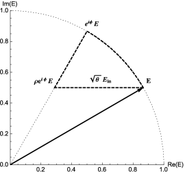
Figure 1: Geometric illustration of a fixed point of Eq.(4). The original vector is reproduced after applying a rotation, a scaling and adding the pump vector. Either one or three stationary states are possibile when the rotation (phase-shift) is assumed small, but additional stationary states can also be obtained if the rotation is by more than one lap.

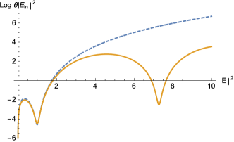
Figure 2: Comparison of pump dependence on the intracavity power for multi-valued stationary continuous wave solutions of the LLE (blue dashed) and the Ikeda map (orange solid). Parameters $\alpha=\theta=0.1$ and $\gamma=L=P_{in}=\delta_{0}=1$.

The corresponding bistable steady-state condition for the LLE (3) is given by

$$\frac{1}{\alpha^{2}+(\delta_{0}-\gamma L|E|^{2})^{2}}=\frac{|E|^{2}}{\theta|E_{in}|^{2}}$$ (6)

A comparison of Eqs.(5-6) is shown in Fig. 2, where it is seen that the LLE (blue dashed curve) is an excellent approximation for small intracavity powers but that it quickly becomes bad as the power increases. Indeed, from Eq.(5) we see that the intracavity power will have a linear asymptotic dependence on $|E|^{2}$, while Eq.(6) for the LLE predicts that the intracavity power should depend asymptotically on the cubic root of the pump power. The intensity inside the resonator will consequently increase much faster than the LLE predicts. From Fig. 2 we also see that higher-order multi-stable (or excited) states do not necessarily imply that the pump power needs to be large. In fact one finds that excited solutions may even coexist with the low-power bistable response.

The successive intracavity powers for which the pump power has a minimum in Fig. 2, i.e., the least pump power needed to reach a state on a given level, can be found explicitly from Eq.(5) as $|E|^{2}=(\delta_{0}+2\pi n)/(\gamma L)$, where $n$ is a positive integer, while the corresponding pump powers are given by $\theta|E_{in}|^{2}=(\delta_{0}+2\pi n)(1-\rho)^{2}/(\gamma L)$. The pump power required to reach the first excited level is thus a fraction $1+2\pi/\delta_{0}$ larger than that required in order to reach the upper level of the bistability curve. Therefore, the observation of excited states is facilitated if the detuning is fairly large. In this article we refer to states with $n\geq 1$ as excited states, since the LLE is only able to model the first minimum occurring for $n=0$.

We now consider the physical parameters necessary to obtain a nonlinear phase-shift of order unity in microresonator devices. The phase condition $\phi_{NL}=\gamma LP_{0}\sim 1$ depends on the intracavity power $P_{0}=|E|^{2}$ rather than the pump power. However, from Eq.(5) one can estimate that the power will grow linearly with the resonator finesse, i.e. $P_{0}\sim P_{in}\mathcal{F}/\pi$. This approximation corresponds to a lower bound for a critically coupled resonator. The phase-shift condition can alternatively be written in terms of the resonator Q-factor and the effective mode area as $\phi_{NL}\approx 2\frac{n_{2}}{n_{0}}\frac{P_{in}Q}{A_{eff}}\sim 1$. The nonlinear phase-shift is related to the Kerr frequency mode shift as $\Delta\nu_{NL}=\phi_{NL}\Delta\nu_{FSR}/(2\pi)$, with a phase-shift of $2\pi$ thus able to shift the field to a different resonance. Note that the modes can also experience a thermally induced mode shift, however, this is not taken into account in the current treatment.

Microresonators featuring large mode shifts have in fact already been experimentally demonstrated in the literature. For example, in Ref. delhaye_octave_2011 a fused silica microtoroid, with a diameter of $80~{}\mu m$ and $Q\approx 2.7\times 10^{8}$, was used to demonstrate octave spanning comb generation. This resonator had a Kerr frequency shift that was estimated to be as much as $100~{}GHz$ at $1~{}W$ of input power, while the FSR of the resonator was $850~{}GHz$. The corresponding nonlinear phase-shift would therefore be $\phi_{NL}\approx 0.74$, which suggests that the mean-field approach may be inaccurate. The comb bandwidth of the same resonator was also theoretically analysed in Ref. coen_universal_2013 , with experimental measurements showing deviations of one order of magnitude from predictions based on the LLE. These large deviations were however attributed to be mainly due to higher-order dispersion.

IV Linear stability analysis

Optical frequency comb generation in microresonators pumped by a CW laser is initiated by the growth of frequency sidebands above a certain threshold power. These sidebands are symmetrically spaced and occur due to modulational instability (MI) of the pump mode. Because of the cavity boundary conditions, MI in a resonator cavity can display qualitatively different features, compared to the conventional MI in a straight waveguide. This is because the detuning between the resonance frequency of the cavity and the pump frequency, introduces an additional degree of freedom for the phase-matching of different four-wave-mixing processes. As a consequence, the steady-state CW solution can become modulationally unstable also in the normal dispersion regime haelterman_additive-modulation-instability_1992 .

An analysis of the linear stability of the steady-state solution in the mean-field limit has been performed by many authors, see e.g. Refs. matsko_optical_2005 ; chembo_modal_2010 ; hansson_dynamics_2013 . However, the LLE does not model the full dynamics of the instabilities that can occur in a resonator cavity described by the Ikeda map. Particularly, one finds that additional unstable frequency bands (resonance tongues) appear at high power. These bands can be associated both with instabilities having the fundamental period and with period doubling instabilities coen_modulational_1997 .

In order to investigate the linear stability of steady-state solutions described by Eq.(5), we assume an ansatz of the form $E^{m}(t,z)=[E_{0}+u^{m}(t,z)+iv^{m}(t,z)]\exp[-\alpha_{i}z/2+i\gamma(1-e^{-\alpha_{i}z})|E_{0}|^{2}/\alpha_{i}+iArg~{}E_{0}]$, where the perturbations $u^{m}(t,z)$ and $v^{m}(t,z)$ are real functions. Linearising the nonlinear Schrödinger Eq.(2) we find that the Fourier transform of the perturbations $w^{m}(z)\equiv[\tilde{u}^{m}(\omega,z),~{}\tilde{v}^{m}(\omega,z)]^{T}$ should satisfy the following system of linear equations $dw^{m}/dz=Mw^{m}$, with the perturbation matrix

$$M(z)=\left[\begin{array}[]{cc}0&-(\beta_{2}/2)\omega^{2}\\ (\beta_{2}/2)\omega^{2}+2\gamma|E_{0}|^{2}e^{-\alpha_{i}z}&0\end{array}\right].$$ (7)

The analytical solution of this system is quite involved in the general case and the stability is most easily investigated numerically. However, in the absence of intrinsic absorption, i.e. $\alpha_{i}\to 0$, the matrix $M$ becomes independent of $z$ and the solution simplifies considerably, see Refs. coen_modulational_1997 ; zezyulin_modulational_2011 . In this case one finds that the eigenvalues of $M$ give the conventional MI gain of a straight waveguide, viz.

$$\mu=\omega\sqrt{-\beta_{2}\gamma|E_{0}|^{2}-(\beta_{2}^{2}/4)\omega^{2}},$$ (8)

while the solution of the linear system is given by

$$w^{m}(z)=\left[\begin{array}[]{cc}-\beta_{2}\omega^{2}e^{\mu z}&-\beta_{2}\omega^{2}e^{-\mu z}\\ 2\mu e^{\mu z}&-2\mu e^{-\mu z}\end{array}\right]\left[\begin{array}[]{c}a_{m}\\ b_{m}\end{array}\right]\equiv W(z)c^{m}$$ (9)

In the next step we consider the boundary condition Eq.(1) that the perturbed solution must satisfy and apply the Fourier transform. This leads to $w^{m+1}(0)=\sqrt{1-\theta}R(\phi)w^{m}(L)$, where $\phi=\phi_{0}+\gamma L|E_{0}|^{2}$ and $R(\phi)$ is the rotation matrix

$$R(\phi)=\left[\begin{array}[]{cc}\cos\phi&-\sin\phi\\ \sin\phi&\cos\phi\end{array}\right].$$ (10)

We then obtain a system of difference equations for the coefficients $c^{m}=[a_{m},~{}b_{m}]^{T}$, viz. $c^{m+1}=\sqrt{1-\theta}[W^{-1}(0)R(\phi)W(L)]c^{m}\equiv Qc^{m}$. The stability of solutions to this linear system of difference equations with constant coefficients depends, similarly to Eq.(7), on the magnitude of the eigenvalues. The Ikeda map has an instability whenever the modulus of an eigenvalue of $Q$ is larger than unity.

For the case when the intrinsic absorption is neglected these eigenvalues are explicitly given by

$$q_{\pm}=\sqrt{1-\theta}(p\pm\sqrt{p^{2}-1})$$ (11)

where $p=\cos(\phi)\cosh(\mu L)-\left[\gamma|E_{0}|^{2}+(\beta_{2}/2)\omega^{2}\right]\sin(\phi)\sinh(\mu L)/\mu$, with $\mu$ given by Eq.(8) and the phase-shift $\phi=\phi_{0}+\gamma L|E_{0}|^{2}$, see Ref. coen_modulational_1997 .

For the general case the stability of the Ikeda map can be determined using a numerical Floquet analysis conforti_modulational_2014 ; bender_advanced_1999 . This is accomplished by investigating the stability of eigenvalues of the fundamental matrix $[w_{1}^{m+1}(0),~{}w_{2}^{m+1}(0)]$. This matrix is obtained by numerically integrating the perturbed system $dw^{m}/dz=M(z)w^{m}$ over one roundtrip, starting from two linearly independent initial conditions, e.g. $w_{1,2}^{m}(0)=[1,~{}0]^{T},[0,~{}1]^{T}$, and applying the boundary condition Eq.(1).

In Figs. 3-4 we show some some examples of modulational instability gain for both anomalous and normal dispersion. The gain has been calculated numerically using the Floquet method for parameters corresponding to the silica resonator of Ref. delhaye_octave_2011 mentioned at the end of section III. Note that even though the magnitude of the intracavity power is very large, the maximum plotted value may actually correspond to pump powers as low as $2~{}W$, owing to the very high finesse $\mathcal{F}\approx 10^{6}$ of the resonator.

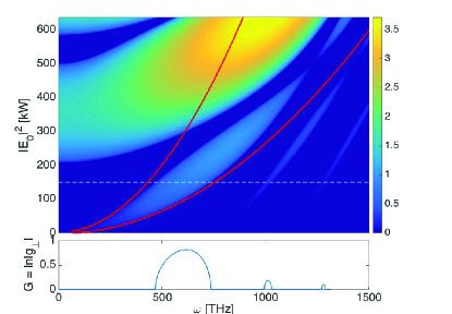
Figure 3: Parametric instability tongues of the Ikeda map for anomalous dispersion. The red contour shows the predicted range of modulational instability for the LLE. Below a cross section corresponding to the dashed line is shown with alternating CW-MI/P2-MI gain bands. Parameters: $\gamma=25~{}W^{-1}km^{-1}$, $L=2\pi\times 40~{}\mu m$, $\mathcal{F}=10^{6}$, $\beta_{2}=-40~{}ps^{2}km^{-1}$ and $\delta_{0}=0$.

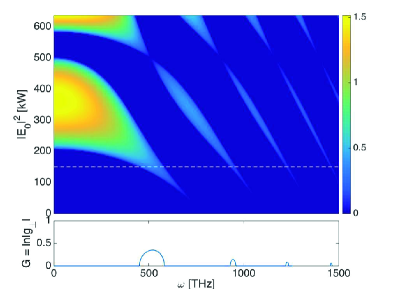
Figure 4: Parametric instability tongues of the Ikeda map for the same parameters as in Fig. 3 but with the sign of the dispersion reversed to give normal dispersion $\beta_{2}=40~{}ps^{2}km^{-1}$. The cross section shows alternating P2-MI/CW-MI gain bands. Note that the LLE does not predict any instability for these parameters.

Fig. 3 shows that the modulational instability analysis for the LLE is valid for low intracavity power, but that new unstable sidebands appear as the power increases. The high power parametric instability tongues may correspond to instabilities occurring for either resonant or anti-resonant conditions. The former includes the ordinary CW-MI of the LLE and higher order sidebands, and has its origin in the $q_{+}$ eigenvalue, while the latter comes from the $q_{-}$ eigenvalue and gives rise to a period doubling instability referred to as P2-MI, see Refs. mclaughlin_new_1985 ; coen_modulational_1997 . The P2-MI can be used to convert a continuous wave solution to a period doubled pattern, i.e. an alternation between two different modulated temporal patterns having a period of one roundtrip each. Since an optical spectrum analyser performs an averaging over many roundtrips, it may be difficult to experimentally distinguish a stable period doubled frequency combs from an ordinary frequency comb.

While the LLE gives a good approximation for the modulational instability gain occurring at low powers, its accuracy becomes increasingly bad as the power increases. Indeed, the LLE is not able to model either P2-MI instabilities nor higher order CW-MI sidebands. Fig. 4 shows that the period doubling instability is in fact usually the first instability to occur for normal dispersion cavities, except for the case when the detuning has been used to compensate for the phase-mismatch. Moreover, we see that high intensity continuous wave solution may actually be stable in certain narrow regions.

The excited continuous wave steady-state solutions generally correspond to the parameter regions which are stable to plane wave perturbations. However, the stability analysis shows that the new states are usually modulationally unstable (CW-MI and/or P2-MI) for anomalous dispersion, similar to the upper steady-state level in the simple bistable case of the LLE. But since the modulational instability only applies to structures that are sufficiently broad in time, it suggests the intriguing possibility of forming cavity solitons associated with these excited multi-stable states. Indeed, this turns out to be possible under appropriate circumstances and we shall see an example of such excited cavity solitons in section VI.

V Period doubled patterns

In this section we give some examples of period doubled patterns. A period doubled CW solution should satisfy a system of equations similar to that of a steady-state fixed point solution, viz.

$$A=\rho e^{i\phi_{B}}B+\sqrt{\theta}E_{in},\qquad B=\rho e^{i\phi_{A}}A+\sqrt{\theta}E_{in}.$$ (12)

Here we have defined the half-period fields as $A=E^{m}$ and $B=E^{m+1}$. The presence of a period doubled fixed point implies that the field satisfies a functional relation of the form $x=F(F(x))$. If the fields in each half-period are equal, i.e. $A=B=E$ (or $x=F(x)$), there is no period doubling and we recover Eq.(4). From Eq.(12) one finds that the two fields are related to each other through the following resonance condition, see Ref. haelterman_period-doubling_1992 ,

$$\frac{A}{1+\rho e^{i\phi_{B}}}=\frac{B}{1+\rho e^{i\phi_{A}}},$$ (13)

where $\phi_{A,B}$ denotes the phase-shift with the nonlinear term evaluated for $A$ or $B$, respectively.

Period doubled states can occur for relatively low intracavity powers $|A|^{2}$ and $|B|^{2}$ if the cavity detuning is close to anti-resonant conditions, i.e. $\phi\approx\pi$. The above condition (13) also shows that period doubling cannot occur in a linear medium since the denominators cancel each other in the absence of a nonlinear phase-shift.

Two coupled conditions for the intracavity power can be derived, viz.

$$\theta|E_{in}|^{2}=|A|^{2}\frac{(1-\rho^{2})^{2}+4\rho^{2}\sin^{2}\left[(\phi_{A}+\phi_{B})/2\right]}{(1+\rho)^{2}-4\rho\sin^{2}(\phi_{B}/2)}$$ (14)

for $A$ and an analogous condition for $B$ which is obtained by interchanging $A$ and $B$ in the above equation. After solving these equations, the fields can be recovered using the relation $A=\sqrt{\theta}E_{in}(1+\rho e^{i\phi_{B}})/(1-\rho^{2}e^{i(\phi_{A}+\phi_{B})})$.

Period doubled CW solutions are usually only obtained for large input pump powers in microresonator systems where the finesse is high. However, other period doubled patterns can be found at rather modest power levels as a result of period doubling instabilities. An example is shown in Fig. 5 for a microresonator with normal cavity dispersion. The period doubled pattern consists of two identical but out of phase patterns that alternate between each roundtrip. The pattern is found to be stable for the considered operating parameters, but it becomes unstable due to the growth of additional sidebands if the pump power is increased further. Note that the spectrum is constant for the current example since only the spectral phase changes between each roundtrip.

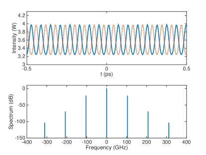
Figure 5: Period doubled pattern obtained through P2-MI instability for normal dispersion resonator. Two identical but out of phase patterns alternate between each roundtrip (blue solid line denotes even numbered roundtrips, red dotted odd). Numerical simulation of the Ikeda map using parameters $\alpha=\theta=0.01$, $\gamma=100~{}W/m$, $L=0.1~{}mm$, $P_{in}=4.5~{}W$, $FSR=100~{}GHz$, $\beta_{2}=500~{}ps^{2}/km$ and $\delta_{0}=0.25$.

VI Localised solutions, cavity solitons

An important question that we have not considered so far is whether or not the Ikeda map has any additional types of localised solutions different from those of the LLE. That the answer to this question should be in the positive can be appreciated from the following line of argument.

It is well known that cavity solitons exist for almost the same range of parameters as the bistable CW solution in microresonators described by the LLE. The reason for this is that a bright cavity soliton consists of a solitary pulse sitting on top of a constant background. This background is a stationary and modulationally stable solution of Eq.(5). Similarly, since cavity solitons are concave at their peak, there should also exist another stationary CW solution that corresponds to two points on the soliton were the second derivative is zero. However, it should be noted that this is only approximately true, due to the phase difference between the soliton and the background. The two points are inflexion points, i.e. points on the soliton profile were the slope of the derivative goes from increasing to decreasing or vice versa. The latter stationary CW level is however not required to be stable against MI as long as the soliton is not too broad. Consequently, it can be understood that one should be in a regime were at least two CW solutions coexist for the same pump parameters in order to find a stationary cavity soliton solution. Similarly, if more than two stationary CW states are present simultaneously, then we can expect that each new level may also be associated with a different cavity soliton state.

To find a cavity soliton associated with an excited CW state we consider operating parameters allowing for three simultaneous steady-state CW levels with positive slope, see Fig. 6. For the numerical simulations we consider a microresonator with parameters $\alpha=\theta=0.01$, $\gamma=100~{}W/m$, $L=0.1~{}mm$, $FSR=100~{}GHz$, $\beta_{2}=-500~{}ps^{2}/km$, $P_{in}=1~{}W$ and $\delta_{0}=0.6$. These parameters are somewhat idealised since we neglect higher order dispersion, but similar parameters could be obtained for semiconductor microrings featuring large nonlinear Kerr coefficients such as e.g. AlGaAs. In Figs. 7-8 we demonstrate a case were two different stable cavity solitons, one conventional LLE soliton and one super cavity soliton associated with an excited state, are obtained and may coexist simultaneously inside the cavity.

Figure 6: Configuration for stationary CW solutions allowing for multi-level cavity solitons. Logarithm of pump power plotted vs. intracavity power. The constant line corresponds to the external pump power ($1~{}W$) used in the examples.

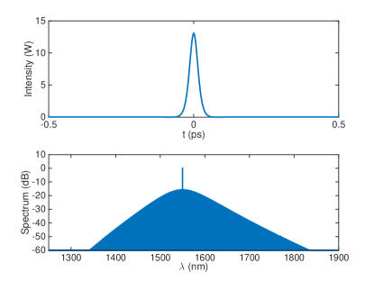
Figure 7: LLE type cavity soliton with background level $|E|^{2}\approx 0.029~{}W$ and support level $|E|^{2}\approx 6.365~{}W$. Simulation of Ikeda map Eqs.(1-2), with parameters $\alpha=\theta=0.01$, $\gamma=100~{}W/m$, $L=0.1~{}mm$, $P_{in}=1~{}W$, $FSR=100~{}GHz$, $\beta_{2}=-500~{}ps^{2}/km$ and $\delta_{0}=0.6$.

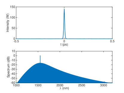
Figure 8: Stationary super cavity soliton with background level $|E|^{2}\approx 0.029~{}W$ and support level $|E|^{2}\approx 68.764~{}W$, using the exact same parameters as in Fig. 7 except for different initial conditions.

The two stationary solitons in Figs. 7-8 are found in the same microring using identical pump parameters. The second cavity soliton that is associated with the excited CW level around $|E|^{2}\approx 68.8~{}W$ in Fig. 6 is seen to be much more energetic than its LLE counterpart, that is associated with the CW power level $|E|^{2}\approx 6.4~{}W$, corresponding to the upper bistable CW solution of the LLE. The soliton shown in Fig. 8 has a peak power that is one order of magnitude greater than that of the LLE soliton. At the same time it is also narrower, leading to a mode-locked frequency comb spectrum that is significantly broader than that of the LLE soliton. This is particularly interesting for applications to broadband frequency comb generation, since such super cavity solitons could easily span a bandwidth of more than an octave, and possibly even multiple octaves with appropriate dispersion engineering. Other potential applications include multi-state optical buffer memories, cf. leo_temporal_2010 .

The intensity of each soliton sans background can be approximated as $|E(t)|^{2}=P_{0}\textrm{sech}^{2}(t/T_{0})$, with peak intensity $P_{0}=2(\delta_{0}+2\pi n)/(\gamma L)$ and temporal duration $T_{0}^{2}=\beta_{2}L/(2(\delta_{0}+2\pi n))$ for $n=0,1$. Note that the two solitons were excited numerically by starting with initial conditions close to the final soliton profile. This corresponds experimentally to the injection of a soliton pulse into the cavity. At present it is not clear how super cavity solitons could best be excited in an experimental setting. This and the relation of super cavity solitons to other types of bistable solitons, cf. kaplan_bistable_1985 , will be the focus of future work.

VII Conclusions

In this article we have presented an analysis of frequency comb generation that goes beyond the mean-field approximation used in the Lugiato-Lefever equation and coupled mode theory. The analysis has been carried out in the context of microresonators but is valid also for dispersive fiber-ring resonators. The LLE is valid only in the limit of small phase-shifts were the nonlinear length scale is much longer than the length of the cavity. Using the more general Ikeda map as a model, we have shown that new multi-valued stationary states appear at high intracavity powers for the CW solution. These states may be present simultaneously as the low power bistable response and do not necessarily require a large pump intensity. The modulational stability of the stationary CW states has been analysed, while taking into account the boundary conditions imposed by the cavity. The stability analysis shows the presence of several parametric instability bands, including period doubling instabilities, at high intracavity power both for normal and anomalous dispersion. An example of how such period doubling instabilities can lead to a stable pattern that alternates between each roundtrip has been demonstrated. Finally, we have predicted a novel type of super cavity soliton solution associated with an excited CW steady-state. These solitons are narrower and more energetic than those of the LLE, allowing for efficient generation of mode-locked ultra wideband frequency combs.

References

- (1) T. J. Kippenberg, R. Holzwarth, and S. A. Diddams, “Microresonator-Based Optical Frequency Combs,” Science 332, 555-559 (2011).
- (2) L. A. Lugiato and R. Lefever, “Spatial dissipative structures in passive optical systems,” Physical Review Letters 58, 2209-2211 (1987).
- (3) S. Coen, H. G. Randle, T. Sylvestre, and M. Erkintalo, “Modeling of octave-spanning Kerr frequency combs using a generalized mean-field Lugiato-Lefever model,” Optics Letters 38, 37-39 (2013).
- (4) Y. K. Chembo and N. Yu, “Modal expansion approach to optical-frequency-comb generation with monolithic whispering-gallery-mode resonators,” Physical Review A 82, 033801 (2010).
- (5) A. B. Matsko, A. A. Savchenkov, W. Liang, V. S. Ilchenko, D. Seidel, and L. Maleki, “Mode-locked Kerr frequency combs,” Optics Letters 36, 2845-2847 (2011).
- (6) P. Del’Haye, A. Coillet, W. Loh, K. Beha, S. B. Papp, and S. A. Diddams, “Phase steps and resonator detuning measurements in microresonator frequency combs,” Nature Communications 6, 5668 (2015).
- (7) H. Nakatsuka, S. Asaka, H. Itoh, K. Ikeda, and M. Matsuoka, “Observation of bifurcation to chaos in an all-optical bistable system,” Physical Review Letters 50, 109-112 (1983).
- (8) R. Vall e, “Temporal instabilities in the output of an all-fiber ring cavity,” Optics Communications 81, 419-426 (1991).
- (9) S. Coen, M. Haelterman, P. Emplit, L. Delage, L. M. Simohamed, and F. Reynaud, “Experimental investigation of the dynamics of a stabilized nonlinear fiber ring resonator,” Journal of the Optical Society of America B 15, 2283-2293 (1998).
- (10) A. Ankiewicz and C. Pask, “Chaos in optics: field fluctuations for a nonlinear optical fibre loop closed by a coupler,” The Journal of the Australian Mathematical Society. Series B. Applied Mathematics 29, 1-20 (1987).
- (11) K. Ikeda, “Multiple-valued stationary state and its instability of the transmitted light by a ring cavity system,” Optics Communications 30, 257-261 (1979).
- (12) M. Haelterman, S. Trillo, and S. Wabnitz, “Dissipative modulation instability in a nonlinear dispersive ring cavity,”’ Optics Communications 91, 401-407 (1992).
- (13) T. Hansson, D. Modotto, and S. Wabnitz, “On the numerical simulation of Kerr frequency combs using coupled mode equations,” Optics Communications 312, 134-136 (2014).
- (14) M. Conforti, A. Mussot, A. Kudlinski, and S. Trillo, “Modulational instability in dispersion oscillating fiber ring cavities,” Optics Letters 39, 4200-4203 (2014).
- (15) P. Del’Haye, T. Herr, E. Gavartin, M. L. Gorodetsky, R. Holzwarth, and T. J. Kippenberg, “Octave Spanning Tunable Frequency Comb from a Microresonator,” Physical Review Letters 107, 063901 (2011).
- (16) S. Coen and M. Erkintalo, “Universal scaling laws of Kerr frequency combs,” Optics Letters 38, 1790-1792 (2013).
- (17) M. Haelterman, S. Trillo, and S. Wabnitz, “Additive-modulation-instability ring laser in the normal dispersion regime of a fiber,” Optics Letters 17, 745-747 (1992).
- (18) A. Matsko, A. Savchenkov, D. Strekalov, V. Ilchenko, and L. Maleki, “Optical hyperparametric oscillations in a whispering-gallery-mode resonator: Threshold and phase diffusion,” Physical Review A 71, 033804 (2005).
- (19) T. Hansson, D. Modotto, and S. Wabnitz, “Dynamics of the modulational instability in microresonator frequency combs,” Physical Review A 88, 023819, (2013).
- (20) S. Coen and M. Haelterman, “Modulational instability induced by cavity boundary conditions in a normally dispersive optical fiber,” Physical Review Letters 79, 4139-4142 (1997).
- (21) D. A. Zezyulin, V. V. Konotop, and M. Taki, “Modulational instability in a passive fiber cavity, revisited,” Optics Letters 36, 4623-4625 (2011).
- (22) C. M. Bender, and S. A. Orszag, “Advanced Mathematical Methods for Scientists and Engineers,” (Springer, New York, 1999).
- (23) D. W. McLaughlin, J. V. Moloney, and A. C. Newell, “New class of instabilities in passive optical cavities,” Physical Review Letters 54, 681-684 (1985).
- (24) M. Haelterman, “Period-doubling bifurcations and modulational instability in the nonlinear ring cavity: an analytical study,” Optics Letters 17, 792-794 (1992).
- (25) F. Leo, S. Coen, P. Kockaert, S.-P. Gorza, P. Emplit, and M. Haelterman, “Temporal cavity solitons in one-dimensional Kerr media as bits in an all-optical buffer,” Nature Photonics 4, 471-476 (2010).
- (26) A. E. Kaplan, “Bistable solitons,” Physical Review Letters 55, 1291-1294 (1985).